


A Study of Adaptive Fractional-Order Total Variational Medical Image Denoising


1
School of Automation and Electrical Engineering, Shenyang Ligong University, Shenyang 110159, China
2
Science and Technology on Electro-Optical Information Security Control Laboratory, Tianjin 300308, China
*
Authors to whom correspondence should be addressed.
Fractal Fract. 2022, 6(9), 508; https://doi.org/10.3390/fractalfract6090508
Submission received: 16 June 2022
/
Revised: 29 August 2022
/
Accepted: 7 September 2022
/
Published: 11 September 2022
(This article belongs to the Special Issue Applications of Fractional Operator in Image Processing and Stability of Control Systems)
Abstract
:Following the traditional total variational denoising model in removing medical image noise with blurred image texture details, among other problems, an adaptive medical image fractional-order total variational denoising model with an improved sparrow search algorithm is proposed in this study. This algorithm combines the characteristics of fractional-order differential operators and total variational models. The model preserves the weak texture region of the image improvement based on the unique amplitude-frequency characteristics of the fractional-order differential operator. The order of the fractional-order differential operator is adaptively determined by the improved sparrow search algorithm using both the sine search strategy and the diversity variation processing strategy, which can greatly improve the denoising ability of the fractional-order differential operator. The experimental results reveal that the model not only achieves the adaptivity of fractional-order total variable differential order, but also can effectively remove noise, preserve the texture structure of the image to the maximum extent, and improve the peak signal-to-noise ratio of the image; it also displays favorable prospects for applications in medical image denoising.
1. Introduction
In recent years, image denoising has become one of the important steps of image processing in medical diagnosis. Denoised medical images can provide reliable analysis data for clinicians who read large numbers of medical images daily [1,2]. Due to the sophistication of medical imaging, which can be easily disturbed by many factors, such as the complexity of the human body and the uneven density of the target medium, it is difficult for traditional image denoising algorithms to achieve positive denoising effects for medical images [3,4,5]. Among many algorithms for image denoising, this paper adopts the total variational algorithm of interest to improve the effectiveness of medical image denoising.
The Total Variational (TV) image denoising algorithm [6] was proposed by Rudin and Osher in 1992. It is a well-known case of applying partial differential equations to image denoising. The TV model suppresses image noise by minimizing the energy function. Yet, the edge direction of the flat area does not exist, and diffusion only along the edge direction will lead to insufficient noise suppression in the flat area. Currently, research scholars have proposed some improved algorithms for medical images based on the traditional variational method [7,8]. However, these improvements still cannot eliminate the “step effect” that results from excessive image smoothing when noise is removed from the image using the variational method. In the past few years, several advanced fractional image processing methods have demonstrated that fractional-order differentiation can enhance the texture details of images nonlinearly. Researchers such as Yan et al. [9] designed a new edge-preserving filter for image decomposition using fractional-order differential operators and regularization terms. Zhang et al. [10] applied fractional-order differential masks to image fusion preprocessing. The gap between low- and high-frequency signals in the source image was widened. This enabled the preservation of the image edges while effectively reducing unreasonable hole tone inside the image. Many research scholars have successfully applied fractional-order calculus theory, combined with TV theory, to image processing. This allowed researchers to effectively alleviate the problem of excessive smoothing in smooth areas of images by variational methods [11,12,13]. Zhang et al. [14] defined a new space of fractional-order bounded variational functions to partition image textures of different scales into different negative Sobolev space functions, and proposed a class of fractional-order multiscale variational models for image denoising. The model more effectively preserved the texture details with little grayscale variation in the smooth region of the image. However, it was difficult to obtain the right order to generate the best result from the denoising model. Numerous scholars have conducted numerous studies on how to determine the fractional order, but all of them have only considered the local features of the image [15,16,17]. Yu et al. [18] presented an approach to adaptively determine the order of fractional-order differentiation by calculating the local variance to reflect the local texture complexity of the image. Ullah et al. [19] proposed a trial-and-error method to adaptively adjust the fractional order so that the fractional-order total variational denoising model yields better denoising results.
Although the work of the above authors can adaptively determine the order of the fractional-order variational model for different regions in an image, these methods are used for specific metrics for a particular image and still have limitations for use in medical imaging. In recent years, swarm intelligence optimization algorithms are gradually being applied to medical image processing [20,21,22,23]. The simplicity of its implementation and its ability to provide an adjustment to the global situation have attracted the attention of an increasing number of scholars. Among them, the sparrow search algorithm is a new swarm optimization method inspired by the foraging and anti-feeding behavior of sparrow colonies [24]. The algorithm is significantly better than both the gray wolf optimization algorithm and the particle swarm optimization algorithm in terms of accuracy, convergence speed, stability, and robustness. Zhang et al. [25] proposed a semi-supervised integrated classifier based on an improved sparrow search algorithm and applied it to lung computed tomography image detection. Xiong et al. [26] proposed a fractional-order chaotic sparrow search algorithm for the enhancement of long-range red film images. Therefore, using the sparrow search algorithm for the denoising of medical images to retain their more detailed information has potential application value.
Based on previous work, an adaptive fractional-order total variational medical image denoising model based on an improved sparrow search algorithm is proposed to retain more texture details of images while denoising. The main difficulties addressed this paper include how to find the appropriate order of medical image denoising in the model and how to avoid the sparrow search algorithm from falling into the local optimum. The main contributions of this article are summarized as follows:
- For medical imaging, a new fractional-order total variational medical image denoising algorithm is proposed, which combines the amplitude-frequency characteristics of the fractional-order differential operators and the denoising advantages of the TV model, effectively mitigating the “step effect” generated by the TV model when denoising;
- An improved sparrow search algorithm that incorporates a sine search strategy and a diversity variation processing strategy is proposed to avoid the optimization algorithm from falling into local optimal solutions. Additionally, a multi-objective fusion maximization fitness function is proposed to comprehensively evaluate the denoising effect of the optimization model;
- For the feature information of medical images, an optimized fractional-order total variational medical image denoising model based on a fused multi-strategy improved sparrow search algorithm is proposed. The optimization model not only possesses robust adaptivity, but also retains more detailed texture information of medical images while denoising, which can provide more information to help clinicians in diagnosis.
The rest of the paper is structured as follows. In Section 2, the TV model and the defined form of fractional-order differentiation are briefly introduced, and a fractional-order total variational model for medical images is given. In Section 3, the main research of this paper is given. In Section 4, the results of the denoising experiment comparison are given. In Section 5, the conclusion is given.
2. Fractional-Order Total Variational Medical Image Denoising
2.1. Total Variational Denoising Model
The TV model preserves the edge information as much as possible. In general, it is common to use unconstrained extreme value models by introducing Lagrange multipliers , defining the minimized energy generalized form as follows:
where is the Lagrange weight parameter; is the image after denoising at ; is the original image at ; is the energy function of ; is the image gradient mode with ; and and denote the gradients of in the and directions, respectively. The first term of Equation (1) is the residual, which guarantees that the retains the main features of the . The second term is the regularization term, which serves to eliminate the noise in the image while maintaining the edge information as far as possible.
By the gradient descent method [27], the partial differential equation of Equation (1) is obtained:
where is the time step, and div is the scatter of . The local coordinate expression is
where denotes the tangential direction of the . From the analysis in Equation (3), it is obtained that the diffusion operator of this model diffuses only along the image edge direction, which has the characteristic of anisotropic diffusion. When denoising flat areas of an image, the “step effect” is caused.
2.2. Fractional-Order Total Variational Medical Image Denoising Model
Fractional-order calculus is an extension of integer-order calculus, which has been in use for more than 300 years [28,29,30]. So far, there are three main expressions for the definition of fractional order differentiation: Riemann–Liouville definition, Grünwald–Letnikov definition, and Caputo definition [31]. For one-dimensional signals , the Riemann–Liouville definition is as follows:
where denotes fractional-order differentiation; denotes fractional order differentiation with ; and denotes the Gamma function. The Caputo is defined as follows,
Both the Riemann–Liouville definition and the Caputo definition use the Cauchy integral formula, which is computationally complex. The Grünwald–Letnikov definition can be converted into convolutional form during numerical implementation, and is more adaptable to image signal processing. Therefore, the definition of Grünwald–Letnikov fractional-order differentiation is adopted in this paper. The Grünwald–Letnikov is defined as follows,
where is the combination parameter.
According to Equation (6), if the period is divided by , . Thus, the fractional differential expression is obtained [32]:
Only the case of is considered in this paper. Under the Grünwald–Letnikov definition, the amplitude-frequency characteristic curves with fractional-order differential orders of 0.2, 0.4, 0.6, 0.8, 1, 1.2, and 1.4 are shown in Figure 1. The amplitude-frequency characteristic is the curve of the amplitude of the system frequency response as a function of frequency. As shown in Figure 1, the frequency response of the fractional-order differential operator is equivalent to a nonlinear filter. Noise with high signal strength in the image will be filtered out. Noise with weak signal strength is also suppressed by its nonlinearity. The fractional-order differential operator enhances the texture details of images by denoising.
As observed in Figure 1, there is some enhancement of the lowfrequency signal as and . However, the enhancement is relatively low compared to the case of . Thus, different fractional orders have different effects on image denoising. By changing the order of the fractional-order according to the different features of different regions, the effective denoising of different regions can be achieved.
For medical images, the structural details and edges of the image are critical, and the loss of important details may cause the doctor to make an incorrect diagnosis. Therefore, distinguishing the details and noise of an image is crucial to medical image denoising algorithms. The complete medical image is divided into detail regions and edge regions. These regional features are represented by different signal values. Due to the fractional-order differential operator enhancing the detail region of the signal with low frequency effectively, the fractional-order differential operator is introduced in this paper and a new fractional-order total variational model is proposed. To achieve better denoising result, replace the first-order differential operator in the regular term of Equation (1) with a fractional-order differential operator, as shown in the following equation:
The new energy function of the TV model for medical image denoising is obtained by introducing the fractional-order differential operator [33], which is the Fractional-order Total Variational (FTV) model:
where is the denoised medical image; is the original medical image; is the dimensional order matrix; ; ; and and denote the -order differentiation of in the , direction.
The fractional-order partial differential equation is obtained by generalizing the partial differential Equation (2) as follows:
From the fractional-order partial differential Equation (10), the model degenerates to the TV model as . Therefore, to solve the model, there is need only to solve for . Ref. [10] defines fractional-order partial differentiation of digital images :
Equation (10) is solved using the difference method. Assuming that the image pixels can be represented as an dimensional matrix, the time step is , the spatial grid size is , and time and space can be discrete as
where , , . Then, the numerical solution of the nonlinear FTV model (10) at pixel after iterations can be calculated by Equation (14):
where the initial condition is with and
3. Fractional-Order Total Variational Model Optimization
In this paper, the framework of the proposed model is presented in Figure 2. An Improved Sparrow Search Algorithm (ISSA) is first designed, which integrates a sinusoidal search strategy and diversity variation processing strategy to avoid falling into local optima during the individual search. Then, the algorithm is introduced into the FTV model, and an adaptive FTV medical image denoising algorithm is proposed to address the problem that the order of the FTV denoising model cannot be determined, and to further improve the adaptivity of the FTV model and to preserve the edges and smoothed areas of the images to a greater extent.
3.1. Improve Sparrow Search Algorithm
The Sparrow Search Algorithm (SSA) was proposed by Xue and Shen in 2020 for solving optimization problems. The algorithm has a high merit-seeking ability and fast convergence [24]. In the standard SSA, a set of sparrows that may represent the optimal solution in the solvable space is first initialized, and the ratio of producers and predators is set. The fitness value is calculated and ranked according to the fitness function. Then, the producers and predators update their positions according to the predation rules. Each time the sparrow’s position is updated, the adaptation value is calculated at that time. Iteration is continued until the optimal value is found or the maximum number of iterations is reached.
The updates of producers’ and predators’ positions in the standard SSA adopt the same update formula with the problem of slow search speed. Therefore, the sinusoidal search strategy is introduced in the optimization algorithm of this paper. It enables the individuals with better adaptation in the original population to search near their original positions, reinforcing the local search ability of the algorithm; the individuals with poor adaptation in the original population can explore far from their positions, strengthening the global search capability of the algorithm. The formula for changing the weight of the sine search strategy is as follows [34]:
where is the minimum value of the weight variation range; is the maximum value of the weight variation range; is the fitness value of the i-th sparrow in the t-th iteration of the population; is the optimal fitness value of the population in the t-th iteration; and is the worst fitness value of the population in the t-th iteration.
Applying the values in the sinusoidal search algorithm strategy to the SSA, assuming that the number of sparrows is and the dimensionality of the medical image denoising model of order to be optimized is , the update formulae for producers and predators of the improved algorithm are obtained as follows:
where denotes the number of iterations and denotes the individual position information of the i-th sparrow in the j-th dimension.
Equation (16) represents the location update of the explorer, where is the maximum number of iterations, is the warning value issued after the predator is detected, is the preset safety threshold, is a random number, is a random number obeying a normal distribution, is a matrix, and each element is .
Equation (17) is the location update of the predator, where denotes the current location with the lowest adaptation, is the location of the predator, is a matrix with each element of the matrix being assigned a random value of or , and .
Equation (18) expresses the position update of a sparrow aware of the danger, where is the optimal position of the population; is the random number of step control parameters obeying a mean of 0 and a variance of 1 in normal steps; is the stochastic number; denotes the current individual fitness value; and denote the current global optimal fitness value and the global worst fitness value, respectively; and is the smallest constant.
To solve the problem that the optimization algorithm is prone to fall into local optimum, the index , which indicates population aggregation in biology, is introduced along with the sinusoidal search strategy. The expression of an indicator is as follows [35]:
where denotes the variance of sparrow population fitness and denotes the mean of sparrow population fitness. The population exhibits an aggregated state as ; when tends to 0, the population exhibits a random state. To avoid the initial appearance of iterations in the aggregated state, the population is treated using the Cauchy variation.
When the value is greater than the preset threshold with , the global optimal solution is mutated using Equation (20):
3.2. Fitness Function
To consider both the quality of the medical image and the similarity with the original image, differentiating from the previous single-objective fitness function, a multi-objective maximization equation is designed as the fitness function of the ISSA algorithm in this paper. In the ISSA algorithm, the value of the fitness function for each sparrow is used to evaluate the denoising effect of medical images. The medical images processed by the ISSA algorithm should filter out most of the noise while retaining the texture structure of the original image. The fitness function is as follows:
where and are constants with and are used to represent the weights of the relative importance of the objective function. Take to ensure a balanced denoising result in this paper.
in Equation (21) represents the peak signal-to-noise ratio (PSNR) [36], and a higher value of PSNR indicates better denoising of the image. The expression formula is as follows:
where denotes the maximum value of the image grayscale; and denote the length and width of the medical image, respectively; denotes the number of pixel points in the medical image; denotes the original medical image; and denotes the denoised medical image.
denotes structural similarity (SSIM) [37], and the higher the SSIM value, the more similar the structure is. The SSIM expression is as follows:
where , , and are defined as:
where and denote the mean values of images and , respectively; and denote the standard deviation of images and , respectively; and denote the variance of images and , respectively; denotes the covariance of images and ; , , are constants; and .
3.3. Steps of the Proposed Denoising Algorithm
A FTV medical image denoising method based on an ISSA is proposed to better filter out medical image noise. Unlike the FTV model with a constant order matrix, the adaptive FTV model proposed in this paper adaptively adjusts the order of each pixel point according to the edge region and detail region of medical images.
The first step is to input the medical image; sparrows are randomly selected and divided into producers and predators in a certain proportion. The fitness value of each sparrow is calculated and ranked according to the objective function (21). Secondly, the location information of each producer and predator is updated according to Equations (16)–(18), and the fitness value of each sparrow is updated according to Equation (21). At the end of the iteration, the order matrix suitable for denoising different features in different regions of the input image is obtained. Finally, the order matrix is substituted into the FTV model (14) to obtain the denoised medical image .
To express the proposed algorithm more clearly, the specific steps of the proposed algorithm are described using a grayscale image of size in Figure 3a as an example. The steps of the ISSA-based Fractional-order Total Variational (ISAFTV) medical image algorithm are as follows:
Step 1: Initialize the FTV model. Input noisy image as shown in Figure 3a. After several tests, the ideal experimental parameters were obtained, where the maximum number of model iterations , step size , and weight coefficient .
Step 2: Initialize the ISSA algorithm. The pixel size of the noisy image is , i.e., the dimension of the optimization problem is and the order matrix to be solved is . The number of sparrows in the population is ; the search range is ; the maximum iteration is set as ; the weights in the sinusoidal search strategy are set as and ; the threshold for sparrows to raise alarm; and the producers and predators are classified according to the of the total proportion of producers.
Step 3: Calculate the PSNR and SSIM of the noisy image. Obtain the fitness values of each sparrow according to the maximum objective function (21) and rank them.
Step 4: Update the location formulae. For producers and predators, update the location information according to Equations (16)–(18).
Step 5: Introduce the diversification variation processing operation and perturb the optimal position using Equation (20) when the aggregation of individuals reaches a specified value.
Step 6: Output ISSA algorithm results. At the end of the loop, the maximum fitness function value is obtained, which is used to find the fractional order for medical image denoising; the visualization of the order matrix is shown in Figure 3b.
Step 7: Output the processed image. The obtained order matrix is substituted into the FTV model (14) to obtain the denoised image as in Figure 3c.
The pseudo-code of the ISAFTV algorithm is shown in Algorithm 1.
| Algorithm 1. Pseudocode for ISAFTV algorithm, ISAFTV |
| Input: Medical image ; FTV model parameters: , , ; ISSA algorithm parameters: order limit range, , , , number of explorers, and . Output: Model order matrix ; denoised image . 1: Read denoised image information; |
| 2: Initialize the population; |
| 3: for to do |
| 4: Calculate the PSNR and SSIM of the denoised image according to Equations (22) and (23); |
| 5: Calculate the fitness value for each sparrow; |
| 6: Sort by fitness value; |
| 7: Update explorer and predator locations with Equations (16)–(18); |
| 8: Calculate population aggregation index ; |
| 9: if then |
| 10: Perturb of the optimal position according to Equation (20); |
| 11: end |
| 12: Obtain the current position; |
| 13: If the new position is better than the previous one, update the optimal position; |
| 14: end |
| 15: Obtain the model order matrix ; 16: for to do 17: Denoising the image according to the fractional order total variational model (14);18: end |
| 19: Output denoised image . |
4. Simulation Experiments and Results Analysis
In this section, Experiment 1 is designed to verify the effect of fractional order on medical image denoising by comparing different orders of the FTV model. Experiment 2 demonstrates that for medical images, the ISAFTV model proposed in the paper retains more detailed information during denoising by comparing it with various denoising models. Experiments were performed with Matlab R2018b on a Windows 10 (64-bit) desktop computer with an Intel Core i5, a 2.90 GHz processor, and 4.0 GB of RAM (Dell, Xiamen, China).
Real images of ophthalmic diseases (vitreous hemorrhage and vitreous mechanization) provided by the hospitals cooperating with the project are selected as the experimental objects. Figure 4a shows the image of vitreous hemorrhage. Due to blood vessel rupture, blood pools in the vitreous cavity, causing blood to escape and collect in the vitreous cavity. Figure 4b shows the vitreous mechanization image. The blood in the vitreous is not absorbed for a long time, and the fibrous membrane is formed by intravitreal mechanization. The experimental images are all in size. Due to the aging of the machine and equipment, the images contain a large quantity of noise, making it difficult for clinicians to form judgments.
4.1. Different Order Comparison Experiment
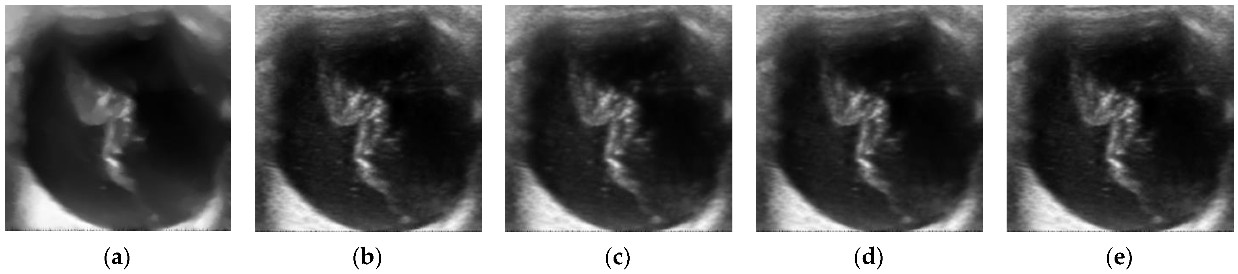
Different orders of FTV models bring different results for medical image denoising. Fractional-order differentiation can nonlinearly enhance the detailed regions of medical images. Compared to and , the fractional order enhances the detail areas of the image more significantly as . In Experiment 1, the results of typical 1-order, 0.4-order, 0.8-order, 1.2-order, and 1.6-order models after denoising the vitreous hemorrhage and vitreous mechanization images are presented in Figure 5 and Figure 6.
Figure 5 and Figure 6 are similar, rendering it difficult to distinguish the denoising effect of different orders, except that the images become blurred after the 1-order model processing. Thus, a quantitative analysis of Table 1 is also needed. Table 1 details the PSNR and SSIM values of vitreous hemorrhage and vitreous mechanization images after processing at different orders in the range of 0 to 2.
From Table 1, it is evident that the results are often not the most desirable with . Overall, the PSNR and SSIM values first increase and then decrease. The optimal denoising effect is . It is further shown that a suitable order helps to improve the denoising effect of the FTV model, as well as to better preserve the textile features of the image.
4.2. Different Model Comparison Experiments
In Experiment 2, the model proposed in this paper is analyzed in a series of comparisons with the TV mode [6], the 0.8-FTV model, the AFOTV model [16], the FNM model [3], and the F-DSG-NLM model [38]. The comparison results reveal that this model retains more details in medical images and provides better assistance to clinicians.
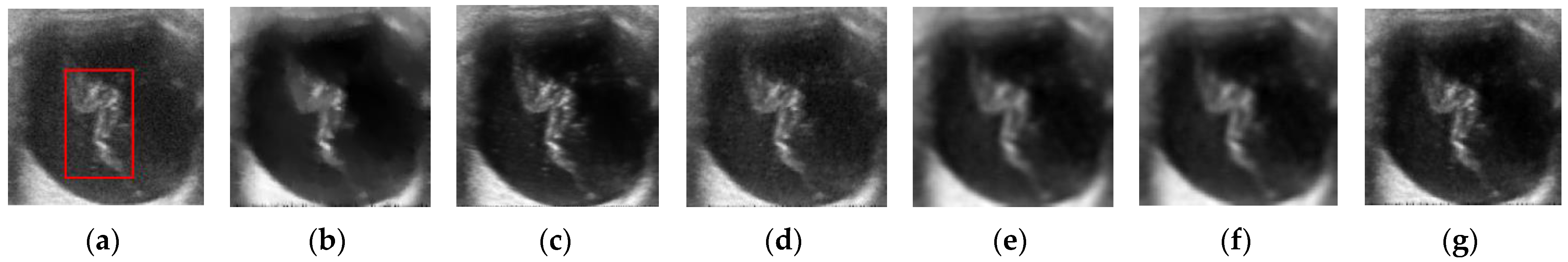
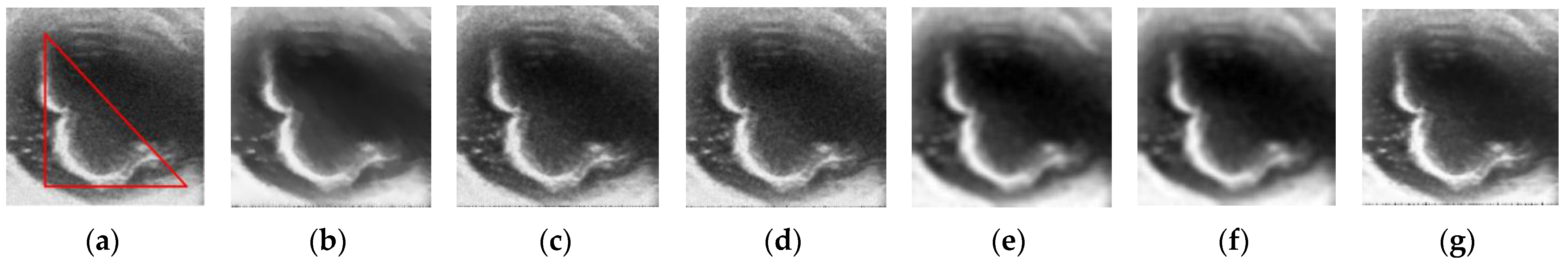
Figure 7, Figure 8, Figure 9 and Figure 10 show the comparative effects of the six denoising models on the denoising of ophthalmic images with the addition of Gaussian noise, with a standard deviation of 15. Figure 7a–g are images of vitreous hemorrhage and Figure 8a–g are magnified views of the portion of the lesion in the red box of Figure 7a, which is a detailed area of the medical image. Figure 9a–g show the vitreous mechanization images and Figure 10a–g show the portion of the lesion within the red box in Figure 9a, which belongs to the marginal area of the medical image. Table 2 and Table 3 show the performance indexes of the images of vitreous hemorrhage and vitreous mechanization corrupted by different degrees of noise after being processed by six denoising models.
Figure 7, Figure 8, Figure 9 and Figure 10 show that all six denoising models can remove the noise from the images to a certain extent. The contours of the lesion portion of the image became sharper after the TV model denoised the vitreous hemorrhage image, as shown in Figure 8b. The image became overall more blurred, as shown in Figure 7b. This is due to the diffusion operator of the TV model only diffusing along the orthogonal direction of the gradient. In processing the vitreous hemorrhage image, there is no edge in the flat area of the image (the hemorrhage portion of the red area in Figure 7a). The TV model over-smoothed the image, resulting in false edges in the blood contour, also known as the “step effect.” The denoising effect of vitreous mechanization images located at the edge is better than that of vitreous hematopoietic images. The PSNR values of vitreous mechanization after the TV model treatment in Table 3 are also higher than those of the vitreous hemorrhage images in Table 2.
The denoising results of the 0.8-FTV model are shown in Figure 7c and Figure 9c. Compared with the TV model, the 0.8-order differentiation preserves the detailed areas of the image nonlinearly, which alleviates the “step effect” caused by the integer differentiation in the TV model by over-smoothing the flat areas of the image. Therefore, it better preserves the detailed information of the blood accumulation in the part of the lesion in the vitreous hemorrhage image, as in Figure 8c. Table 2 and Table 3 show that the PSNR values as well as the SSIM values of the images processed by the 0.8-FTV model are higher than those of the TV model, but the order of the fractional order often requires many experiments to obtain, and the artificially selected order is only a constant, which cannot adapt to different feature points of different images, resulting in incomplete image noise removal and incomplete detail retention.
The AFOTV model achieves order adaptation by Bregman iteration according to the features of the image compared to the 0.8-FTV model. However, Figure 7d and Figure 9d show that the denoising effect of this model is not significantly different from that of the 0.8-FTV model.
Figure 7e and Figure 9e show the denoising results of the F-DSG-NLM model for two diseases, and Figure 7f and Figure 9f show the denoising results of the FNM model. Both models are improvements to the non-local denoising algorithm. It can be observed from the denoising result plots that the images become more blurred after the denoising of the ophthalmic ultrasound images for both types of images, which destroys the detailed information inside the vitreous in the images. It is proven that traditional image denoising methods do not apply to medical images.
The denoising results of the model in this paper for two disease images are shown in Figure 7g and Figure 9g. The noise in the image is largely eliminated in both the detailed area of vitreous hemorrhage and the edge area of vitreous mechanization. The detailed information in the image is also retained. This is because the adaptive search for the optimal order of fractional-order for different regions of the whole image using the ISSA algorithm improves the denoising ability of the fractional-order differential operator and overcomes the loss of image detail information, thus obtaining better visual results and helping doctors to diagnose diseases more efficiently and correctly.
In the numerical analysis of two disease images with Table 2 and Table 3, six denoising models outperform medical image denoising for medical images with low noise intensity than those with high noise intensity. The PSNR values of the proposed model for medical image denoising are better than other models regardless of the variation of noise intensity. Experiments prove that the proposed model in this paper has a positive denoising effect. Meanwhile, the SSIM values of the TV model and the FTV model for the two disease images after denoising are generally kept above 0.7, and the SSIM values of the AFOTV model, FNM model, and F-DSG-NLM model for image denoising generally remain around 0.8, while the SSIM values of this model for the medical images with a standard deviation of 10 added remain above 0.85 overall, and the SSIM values of the images with standard deviations of 15 and 20 added are always kept around 0.8, indicating that the details of the image structure after denoising of this model remain intact. The combined Table 2 and Table 3 demonstrate the effectiveness of the proposed model for ophthalmic ultrasound image denoising.
5. Conclusions
The adaptive FTV medical image denoising model better protects the sharp edges of the image, highlights the focal part of the patient, has a better balance between removing noise and protecting image features, and compensates for the shortcomings of the TV model in processing images. Meanwhile, the introduction of the ISSA algorithm avoids the artificial selection of a fractional-order differential order, improves the denoising ability of a fractional-order differential operator, and realizes the adaptiveness of a fractional-order differential operator. Finally, this paper verifies the effectiveness of this model by comparing the denoising effect of ultrasound images of two ophthalmic diseases.
In future research, we will focus on Ref. [9] to accurately distinguish the detailed regions as well as the edge regions of medical images by use of a fractional-order differential Sobel edge operator so that more detailed information can be retained in the process of the denoising of medical images to provide more help for clinicians. In addition, the additional term added to the regular term in Ref. [9] is able to attenuate the effect of the infrared background and provide us with new research ideas. Later, we will also consider the application of the proposed model with the additional term in Ref. [9] to the denoising of complex infrared images, and thus seek to improve the utility of the proposed model.
Author Contributions
Conceptualization, methodology, software, validation, Y.Z., T.L. and F.Y.; formal analysis, Y.Z.; investigation, F.Y.; resources, Y.Z. and F.Y.; writing—original draft preparation, T.L.; writing—review and editing, Y.Z.; visualization, F.Y.; supervision, Y.Z. and Q.Y.; project administration, Y.Z. and F.Y.; funding acquisition, Y.Z. All authors have read and agreed to the published version of the manuscript.
Funding
This research was funded by Liaoning Provincial Education Department Scientific Research Project (LJKZ0245) and National Key Laboratory Project (2021JCJQLB055006).
Institutional Review Board Statement
The study was conducted in accordance with the Declaration of Helsinki, and approved by the Ethical Committee of the Fourth Affiliated Hospital of China Medical University (EC-2021-HY-035 and 21 June 2021).
Informed Consent Statement
Informed consent was obtained from all subjects involved in the study.
Data Availability Statement
Not applicable.
Acknowledgments
Thanks to Mingyu Shi for providing the experimental images.
Conflicts of Interest
The authors declare no conflict of interest.
References
- Steuwe, A.; Valentin, B.; Bethge, O.T.; Ljimani, A.; Niegisch, G.; Antoch, G.; Aissa, J. Influence of a deep learning noise reduction on the CT values, image noise and characterization of kidney and ureter stones. Diagnostics 2022, 12, 1627. [Google Scholar] [CrossRef] [PubMed]
- Brendlin, A.S.; Schmid, U.; Plajer, D.; Chaika, M.; Mader, M.; Wrazidlo, R.; Männlin, S.; Spogis, J.; Estler, A.; Esser, M.; et al. AI denoising improves image quality and radiological workflows in pediatric ultra-low-dose thorax computed tomography scans. Tomography 2022, 8, 1678–1689. [Google Scholar] [CrossRef] [PubMed]
- Darbon, J.; Cunha, A.; Chan, T.F.; Osher, S.; Jensen, G.J. Fast nonlocal filtering applied to electron cryomicroscopy. In Proceedings of the IEEE International Symposium on Biomedical Imaging: From Nano to Macro, Paris, France, 14–17 May 2008. [Google Scholar]
- Parrilli, S.; Poderico, M.; Angelino, C.V.; Verdoliva, L. A nonlocal SAR image denoising algorithm based on LLMMSE wavelet shrinkage. IEEE Trans. Geosci. Remote Sens. 2012, 50, 606–616. [Google Scholar] [CrossRef]
- Mustafi, A.; Ghorai, S.K. A novel blind source separation technique using fractional Fourier transform for denoising medical images. Optik 2013, 124, 265–271. [Google Scholar] [CrossRef]
- Rudin, L.I.; Osher, S.; Fatemi, E. Nonlinear total variation based noise removal algorithms. Phys. D 1992, 60, 259–268. [Google Scholar] [CrossRef]
- Duan, J.; Lu, W.; Tench, C.; Gottlob, I.; Proudlock, F.; Samani, N.N.; Bai, L. Denoising optical coherence tomography using second order total generalized variation decomposition. Biomed. Signal Process. Control 2016, 24, 120–127. [Google Scholar] [CrossRef]
- Fu, Y.; Liu, J.; Xu, J.; Gu, D.; Yang, K. Ultrasonic images denoising based on calculus of variations. In Proceedings of the 2019 IEEE 4th International Conference on Signal and Image Processing (ICSIP), Wuxi, China, 19–21 July 2019; pp. 970–974. [Google Scholar]
- Yan, H.; Zhang, J.X.; Zhang, X.F. Injected infrared and visible image fusion via L1 decomposition model and guided filtering. IEEE Trans. Comput. Imaging 2022, 8, 162–173. [Google Scholar] [CrossRef]
- Zhang, X.F.; He, H.; Zhang, J.X. Multi-focus image fusion based on fractional order derivative and closed image matting. ISA Trans. 2022. [Google Scholar] [CrossRef]
- Zhang, X.; Huang, W. Adaptive neural network sliding mode control for nonlinear singular fractional order systems with mismatched uncertainties. Fractal Fract. 2020, 4, 50. [Google Scholar] [CrossRef]
- Zhang, X.; Dai, L. Image enhancement based on rough set and fractional order differentiator. Fractal Fract. 2022, 6, 214. [Google Scholar] [CrossRef]
- Wang, D.; Nieto, J.J.; Li, X.; Li, Y. A spatially adaptive edge-preserving denoising method based on fractional-order variational PDEs. IEEE Access 2020, 8, 163115–163128. [Google Scholar] [CrossRef]
- Zhang, J.; Wei, Z. A class of fractional-order multi-scale variational models and alternating projection algorithm for image denoising. Appl. Math. Model. 2011, 35, 2516–2528. [Google Scholar]
- Rojas, H.E.; Cortés, C.A. Denoising of measured lightning electric field signals using adaptive filters in the fractional fourier domain. Measurement 2014, 55, 616–626. [Google Scholar] [CrossRef]
- Li, D.; Tian, X.; Jin, Q.; Hirasawa, K. Adaptive fractional-order total variation image restoration with split Bregman iteration. ISA Trans. 2018, 82, 210–222. [Google Scholar] [CrossRef]
- Thanh, D.N.; Hien, N.N.; Prasath, S. Adaptive total variation L1 regularization for salt and pepper image denoising. Optik 2020, 208, 163677. [Google Scholar] [CrossRef]
- Yu, J.; Tan, L.; Zhou, S.; Wang, L.; Wang, C. Image denoising based on adaptive fractional order anisotropic diffusion. KSII Trans. Internet Inf. Syst. (TIIS) 2017, 11, 436–450. [Google Scholar]
- Ullah, A.; Chen, W.; Khan, M.A. A new variational approach for restoring images with multiplicative noise. Comput. Math. Appl. 2016, 71, 2034–2050. [Google Scholar] [CrossRef]
- Zhang, X.; Liu, R.; Ren, J.; Gui, Q. Adaptive fractional image enhancement algorithm based on rough set and particle swarm optimization. Fractal Fract. 2022, 6, 100. [Google Scholar] [CrossRef]
- Asha, C.S.; Lal, S.; Gurupur, V.P.; Saxena, P.P. Multi-modal medical image fusion with adaptive weighted combination of NSST bands using chaotic grey wolf optimization. IEEE Access 2019, 7, 40782–40796. [Google Scholar] [CrossRef]
- Li, K.S.; Tan, Z.P. An improved flower pollination optimizer algorithm for multilevel image thresholding. IEEE Access 2019, 7, 165571–165582. [Google Scholar] [CrossRef]
- Abdel-Basset, M.; Fakhry, A.E.; El-Henawy, I.; Qiu, T.; Sangaiah, A.K. Feature and intensity based medical image registration using particle swarm optimization. J. Med. Syst. 2017, 41, 197. [Google Scholar] [CrossRef] [PubMed]
- Xue, J.; Shen, B. A novel swarm intelligence optimization approach: Sparrow search algorithm. Syst. Sci. Control Eng. 2020, 8, 22–34. [Google Scholar] [CrossRef]
- Zhang, J.; Xia, K.; He, Z.; Yin, Z.; Wang, S. Semi-supervised ensemble classifier with improved sparrow search algorithm and its application in pulmonary nodule detection. Math. Probl. Eng. 2021, 2021, 6622935. [Google Scholar] [CrossRef]
- Xiong, Q.; Zhang, X.; He, S.; Shen, J. Fractional-order chaotic sparrow search algorithm for enhancement of long distance iris image. Mathematics 2021, 9, 2790. [Google Scholar] [CrossRef]
- Yang, H.; Amari, S. Complexity issues in natural gradient descent method for training multilayer perceptrons. Neural Comput. 1998, 10, 2137–2157. [Google Scholar] [CrossRef] [PubMed]
- Li, R.; Zhang, X. Adaptive sliding mode observer design for a class of T–S fuzzy descriptor fractional order systems. IEEE Trans. Fuzzy Syst. 2020, 28, 1951–1960. [Google Scholar] [CrossRef]
- Zhang, X.; Dong, J. LMI criteria for admissibility and robust stabilization of singular fractional-order systems possessing poly-topic uncertainties. Fractal Fract. 2020, 4, 58. [Google Scholar] [CrossRef]
- Zhang, X.; Yan, Y. Admissibility of fractional order descriptor systems based on complex variables: An LMI approach. Fractal Fract. 2020, 4, 8. [Google Scholar] [CrossRef]
- Yang, Q.; Chen, D.; Zhao, T.; Chen, Y. Fractional calculus in image processing: A review. Fract. Calc. Appl. Anal. 2016, 19, 1222–1249. [Google Scholar] [CrossRef]
- Zhang, X.; Chen, Y. Admissibility and robust stabilization of continuous linear singular fractional order systems with the fractional order α: The 0 < α < 1 case. ISA Trans. 2018, 82, 42–50. [Google Scholar]
- Chen, D.; Chen, Y.; Xue, D. Fractional-order total variation image denoising based on proximity algorithm. Appl. Math. Comput. 2015, 257, 537–545. [Google Scholar] [CrossRef]
- Feng, Z.K.; Niu, W.J.; Liu, S.; Luo, B.; Miao, S.M.; Liu, K. Multiple hydropower reservoirs operation optimization by adaptive mutation sine cosine algorithm based on neighborhood search and simplex search strategies. J. Hydrol. 2020, 59, 125223. [Google Scholar] [CrossRef]
- Laguna, E.; Barasona, J.A.; Triguero-Ocaña, R.; Mulero-Pázmány, M.; Negro, J.J.; Vicente, J.; Acevedo, P. The relevance of host overcrowding in wildlife epidemiology: A new spatially explicit aggregation index. Ecol. Indic. 2018, 84, 695–700. [Google Scholar] [CrossRef]
- Singh, A.; Sethi, G.; Kalra, G.S. Spatially adaptive image denoising via enhanced noise detection method for grayscale and color images. IEEE Access 2020, 8, 112985–113002. [Google Scholar] [CrossRef]
- Wang, Z.; Bovik, A.C.; Sheikh, H.R.; Simoncelli, E.P. Image quality assessment: From error visibility to structural similarity. IEEE Trans. Image Process 2004, 13, 600–612. [Google Scholar] [CrossRef] [Green Version]
- Unni, V.S.; Ghosh, S.; Chaudhury, K.N. Linearized ADMM and fast nonlocal denoising for efficient plug-and-play restoration. In Proceedings of the IEEE Global Conference on Signal and Information Processing, Anaheim, CA, USA, 26–29 November 2018; pp. 11–15. [Google Scholar]
Figure 1.
Fractional-order differential operator amplitude-frequency characteristic curve.

Figure 2.
The framework of the proposed algorithm.

Figure 3.
ISAFTV algorithm simulation example. (a) Step 1 input noisy image. (b) Step 6 output of order matrix visualization image. (c) Step 7 output processed image.
Figure 3.
ISAFTV algorithm simulation example. (a) Step 1 input noisy image. (b) Step 6 output of order matrix visualization image. (c) Step 7 output processed image.

Figure 4.
Experimental images. (a) Vitreous hemorrhage. (b) Vitreous mechanization.

Figure 5.
Results of vitreous hemorrhage image processing by different orders of denoising model. (a) . (b) . (c) . (d) . (e) .
Figure 5.
Results of vitreous hemorrhage image processing by different orders of denoising model. (a) . (b) . (c) . (d) . (e) .

Figure 6.
Results of vitreous mechanization image processing by different orders of denoising model. (a) . (b) . (c) . (d) . (e) .
Figure 6.
Results of vitreous mechanization image processing by different orders of denoising model. (a) . (b) . (c) . (d) . (e) .

Figure 7.
Denoising results of different models after adding Gaussian noise with a standard deviation of 15 to vitreous hemorrhage images. (a) Noise image, the red marked area is the part of the lesion. (b) TV model, run 0.4839 s. (c) FTV model, run 0.5005 s. (d) AFOTV model, run 0.3895 s. (e) F-DSG-NLM model, run 0.0747 s. (f) FNM model, run 14.4760 s. (g) Our model, run 391.6041 s.

Figure 8.
Magnified image of vitreous hemorrhage in part of the lesion. (a) Noise image. (b) TV model. (c) FTV model. (d) AFOTV model. (e) F-DSG-NLM model. (f) FNM model. (g) Our model.
Figure 8.
Magnified image of vitreous hemorrhage in part of the lesion. (a) Noise image. (b) TV model. (c) FTV model. (d) AFOTV model. (e) F-DSG-NLM model. (f) FNM model. (g) Our model.

Figure 9.
Denoising results of different models after adding Gaussian noise with a standard deviation of 15 to vitreous mechanization images. (a) Noise image, the red marked area is the part of the lesion. (b) TV model, run 0.4956 s. (c) FTV model, run 0.9436 s. (d) AFOTV model, run 0.5095 s. (e) F-DSG-NLM model, run 0.3067 s. (f) FNM model, run 14.2753 s. (g) Our model, run 358.1444 s.

Figure 10.
Magnified image of vitreous mechanization in part of the lesion. (a) Noise image. (b) TV model. (c) FTV model. (d) AFOTV model. (e) F-DSG-NLM model. (f) FNM model. (g) Our model.
Figure 10.
Magnified image of vitreous mechanization in part of the lesion. (a) Noise image. (b) TV model. (c) FTV model. (d) AFOTV model. (e) F-DSG-NLM model. (f) FNM model. (g) Our model.


Table 1.
Evaluation index of the image after denoising of different orders .
| Order | Vitreous Hemorrhage | Vitreous Mechanization | ||
|---|---|---|---|---|
| PSNR | SSIM | PSNR | SSIM | |
| 0.2 | 30.2744 | 0.9806 | 32.7779 | 0.9655 |
| 0.4 | 31.0549 | 0.9904 | 33.5478 | 0.9934 |
| 0.6 | 31.0656 | 0.9841 | 33.6727 | 0.9838 |
| 0.8 | 31.6578 | 0.9978 | 34.9359 | 0.9920 |
| 1.0 | 25.1980 | 0.7818 | 26.6687 | 0.7953 |
| 1.2 | 31.5042 | 0.9967 | 34.6754 | 0.9943 |
| 1.4 | 31.4595 | 0.9935 | 34.5923 | 0.9904 |
| 1.6 | 31.4362 | 0.9941 | 34.1148 | 0.9871 |
| 1.8 | 31.1416 | 0.9976 | 33.7817 | 0.9715 |
Table 2.
Objective evaluation criteria of different models for the denoising effect of vitreous hemorrhage images.
Table 2.
Objective evaluation criteria of different models for the denoising effect of vitreous hemorrhage images.
| Standard Deviation | 10 | 15 | 20 | |||
|---|---|---|---|---|---|---|
| PSNR | SSIM | PSNR | SSIM | PSNR | SSIM | |
| Noise image | 28.1391 | 0.6574 | 24.5870 | 0.4819 | 22.1206 | 0.3670 |
| TV model | 25.6914 | 0.7989 | 26.1665 | 0.7995 | 25.9783 | 0.7579 |
| FTV model | 29.0345 | 0.8836 | 27.8864 | 0.7957 | 26.0211 | 0.6750 |
| AFOTV model | 29.7141 | 0.8131 | 27.8282 | 0.8051 | 26.6172 | 0.7236 |
| F-DSG-NLM model | 29.7963 | 0.8376 | 29.3433 | 0.8160 | 28.9241 | 0.7897 |
| FNM model | 29.8856 | 0.8388 | 29.2419 | 0.8163 | 28.8017 | 0.7898 |
| Our model | 30.4862 | 0.8857 | 29.7705 | 0.8331 | 28.9800 | 0.7995 |
Table 3.
Objective evaluation criteria of different models for the denoising effect of vitreous mechanization images.
Table 3.
Objective evaluation criteria of different models for the denoising effect of vitreous mechanization images.
| Standard Deviation | 10 | 15 | 20 | |||
|---|---|---|---|---|---|---|
| PSNR | SSIM | PSNR | SSIM | PSNR | SSIM | |
| Noise image | 28.1928 | 0.6497 | 24.6366 | 0.4825 | 22.1240 | 0.3658 |
| TV model | 25.9562 | 0.8034 | 26.4000 | 0.8007 | 26.2366 | 0.7586 |
| FTV model | 28.9670 | 0.8582 | 27.4736 | 0.7478 | 26.6295 | 0.7266 |
| AFOTV model | 29.8894 | 0.8290 | 28.0774 | 0.8212 | 26.9852 | 0.7449 |
| F-DSG-NLM model | 32.7222 | 0.8790 | 29.0509 | 0.8594 | 27.3167 | 0.7348 |
| FNM model | 32.7744 | 0.8796 | 29.0377 | 0.8595 | 27.2980 | 0.7349 |
| Our model | 33.8371 | 0.9532 | 30.7497 | 0.8614 | 27.7744 | 0.7635 |
Publisher’s Note: MDPI stays neutral with regard to jurisdictional claims in published maps and institutional affiliations. |
© 2022 by the authors. Licensee MDPI, Basel, Switzerland. This article is an open access article distributed under the terms and conditions of the Creative Commons Attribution (CC BY) license (https://creativecommons.org/licenses/by/4.0/).
Share and Cite
MDPI and ACS Style
Zhang, Y.; Liu, T.; Yang, F.; Yang, Q. A Study of Adaptive Fractional-Order Total Variational Medical Image Denoising. Fractal Fract. 2022, 6, 508. https://doi.org/10.3390/fractalfract6090508
AMA Style
Zhang Y, Liu T, Yang F, Yang Q. A Study of Adaptive Fractional-Order Total Variational Medical Image Denoising. Fractal and Fractional. 2022; 6(9):508. https://doi.org/10.3390/fractalfract6090508
Chicago/Turabian StyleZhang, Yanzhu, Tingting Liu, Fan Yang, and Qi Yang. 2022. "A Study of Adaptive Fractional-Order Total Variational Medical Image Denoising" Fractal and Fractional 6, no. 9: 508. https://doi.org/10.3390/fractalfract6090508