
Examining the Position of Wright’s Fallingwater in the Context of His Larger Body of Work: An Analysis Using Fractal Dimensions


1
College of Engineering, Science and Environment, The University of Newcastle, Callaghan 2308, Australia
2
School of Built Environment, The University of New South Wales, Sydney 2052, Australia
*
Author to whom correspondence should be addressed.
Fractal Fract. 2022, 6(4), 187; https://doi.org/10.3390/fractalfract6040187
Submission received: 7 March 2022
/
Revised: 24 March 2022
/
Accepted: 24 March 2022
/
Published: 27 March 2022
(This article belongs to the Special Issue Fractals in the Built Environment: Applications of Fractal Theory to Design and Building)
Abstract
:Frank Lloyd Wright, one of the world’s most famous architects, produced several masterworks in his career, possibly the most celebrated of which is the Kaufmann House, better known as Fallingwater. One of the common arguments historians make about this house is that it is unique in Wright’s oeuvre, as it is not similar to other designs he produced in the three major styles that dominated his career: the Prairie, Textile-Block and Usonian styles. In this paper, the derived fractal dimensions (D) using the standard architectural variation and application of the box-counting method are developed for the elevations and plans of Fallingwater. Using the measurements derived from a set of 15 Prairie, Textile-Block and Usonian houses, this paper tests whether Fallingwater is indeed an outlier in his body of work, as some historians suggest. The results indicate that, contrary to the standard view, Fallingwater has D measures that are broadly similar to those of his other styles, and on average, Fallingwater has formal parallels to several aspects of Wright’s Usonian style.
1. Introduction
Frank Lloyd Wright has been described as ‘America’s most celebrated architect’ [1] (p. 281). He pioneered an alternative version of modern design that ‘would change the face of architecture in the world’ [2] (p. 13). Such is the significance of Wright’s legacy that his designs are still analyzed today, and thousands of scholarly works have been published about his architecture and theories. However, the vast majority of the published research consists of qualitative interpretations of Wright’s architecture with only a comparatively small amount of quantitative analysis [3,4].
One of Wright’s most famous houses, the Kaufmann House or Fallingwater, sits above a waterfall on a stream in Bear Run Nature Reserve in Mill Run, PA, USA. This house, which is famous for being merged into its natural setting, has been the subject of extensive qualitative research and speculation, much of it associated with how this design fits in with Wright’s larger body of work. For example, historians have classified Wright’s domestic designs into three stylistic periods; the Prairie, Textile-Block and Usonian. Fallingwater, however, appears to defy this tripartite classification and is often described by scholars as representing a break from Wright’s usual approach to domestic design. The argument that Fallingwater does not fit neatly within these other stylistic periods seems to be widely accepted by scholars, although there is no quantitative evidence in support of it.
Using the box-counting method for measuring fractal dimensions, this paper measures the formal properties of Wright’s 1937 Fallingwater to determine if they are typical or atypical of his early and mid-career housing (1901–1955). Fractal dimensions have been used previously to measure the formal properties of sets of canonical works from Wright’s three stylistic periods [5]. The results of these computational studies demonstrate that the different stylistic properties of Wright’s architecture can be mathematically categorised using the box-counting method. In the present context, by calculating and comparing the fractal dimensions of plans and elevations of Fallingwater with previously published fractal dimensions of fifteen houses from Wright’s Prairie, Textile-Block and Usonian styles (1901–1955), any differences or similarities can be uncovered. Such a mathematical comparison has not been undertaken of Fallingwater before, and it is significant because it can be used to illuminate a famous argument about the place of Fallingwater in Wright’s oeuvre.
2. Background to the Research
2.1. The Positioning of Fallingwater in Wright’s Architectural Styles
Wright designed Fallingwater in the 1930s as a county retreat for the Kaufmann family. Hailed as a significant architect for his early domestic buildings, many scholars have noted that when Wright designed Fallingwater, he had received no major commissions for several years [6,7,8]. The last designs Wright had completed prior to Fallingwater were the Lloyd Jones House in 1929—the final work of his Textile-Block period—and in 1933, a small residence in Minnesota, an early example of his Usonian style. The stock market crash of 1929 had halted the construction of many of Wright’s designs until 1934, when the Kaufmann family commissioned him to design Fallingwater.
Completed in 1937, Fallingwater is a three-storey house made from what Aaron Green describes as a ‘unique’ combination of specially cut and laid local stone stacked with large rendered concrete cantilevering balconies [9] (p. 136). Dramatically, the waters of Bear Run creek travel under the house and then emerge from beneath the living room terrace, pouring down a series of waterfall ledges. When describing Fallingwater, architectural historians frequently claim that it is a stand-alone house, unique among Wright’s domestic oeuvre, what Diane Maddex describes as a ‘one-of-a-kind’ design [10] (p. 7). Such arguments are founded in a widely held belief that, during his career Wright typically worked in a series of three distinctive styles.
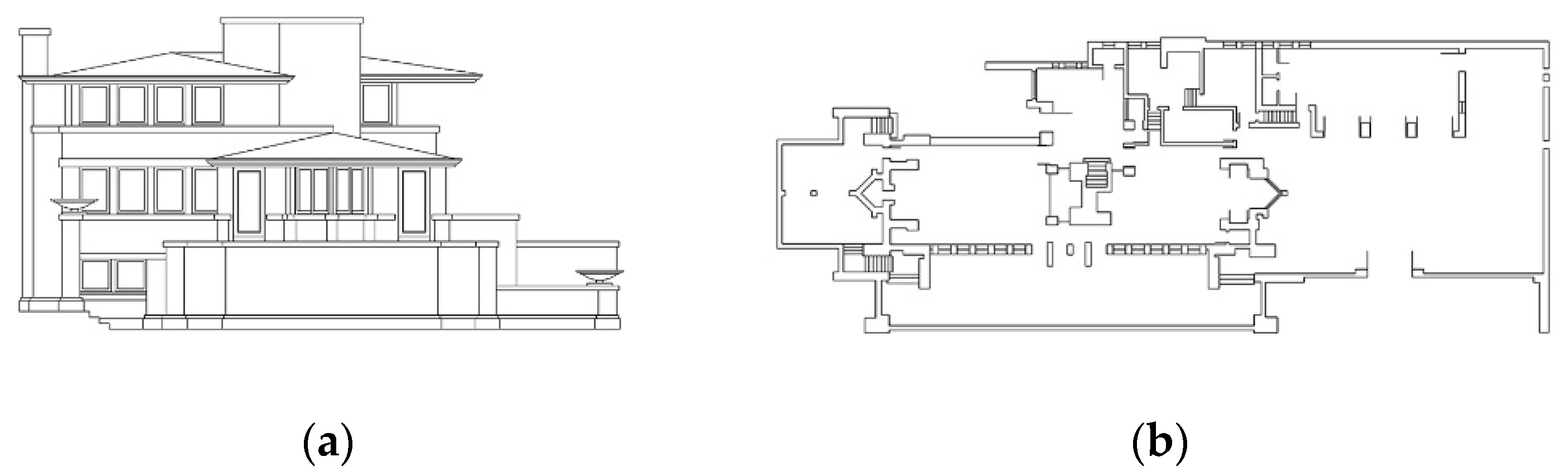
Wright initially gained international recognition for the first of these, his Prairie style. These long, low-lying buildings were designed from the turn of the 20th century as a reflection of the broad expanse of the prairie plains. The Prairie-style houses are characterized by strong horizontal lines and low-pitched roofs over an open interior centered on a hearth. Wright’s 1909 Robie House is often regarded as the most famous example of this approach (Figure 1).
Despite its initial success, Wright’s focus on the Prairie Style began to wane after 1910. In that year he toured Europe and had two portfolios of his work published, seemingly signaling the end of that particular stage in his career. In 1911, his mother purchased a lot for him in Wisconsin, which he named Taliesin. By 1912, Wright had set up his new home and studio at Taliesin and the next decade was spent in experimentation with form, construction methods and mass production.
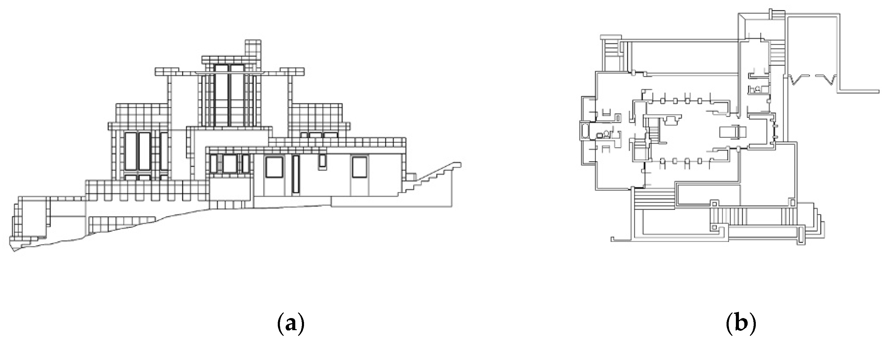
Relocating to Los Angeles in the 1920s, Wright began to think about an alternative masonry system of construction that was appropriate for his new location and during the following decade, he designed multiple buildings, although only five houses were constructed. These five, which have since become known as the Textile-Block homes (Figure 2), were typically constructed from pre-cast patterned and plain exposed concrete blocks connected by steel rods and concrete grout. The plain square blocks of the houses are generally punctuated by ornamented blocks and for each house, a different block-pattern was employed.
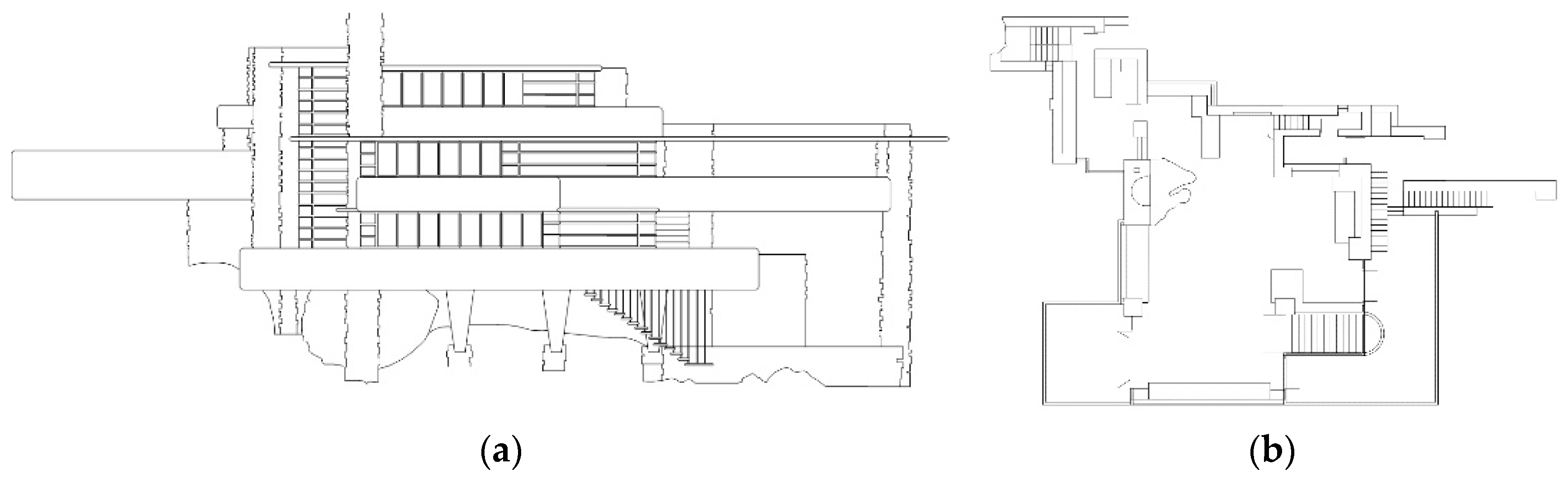
The last house of the Textile-Block period, the Lloyd Jones House in Tulsa (1929), was also Wright’s last major completed commission before Fallingwater (Figure 3). When Fallingwater was revealed to the public, it came as a surprise, being viewed as a dramatic departure from his earlier works, at variance to other architectural styles of the time [6,11], and with a unique appearance that was ‘revolutionary’ at the time [12] (p. 6).
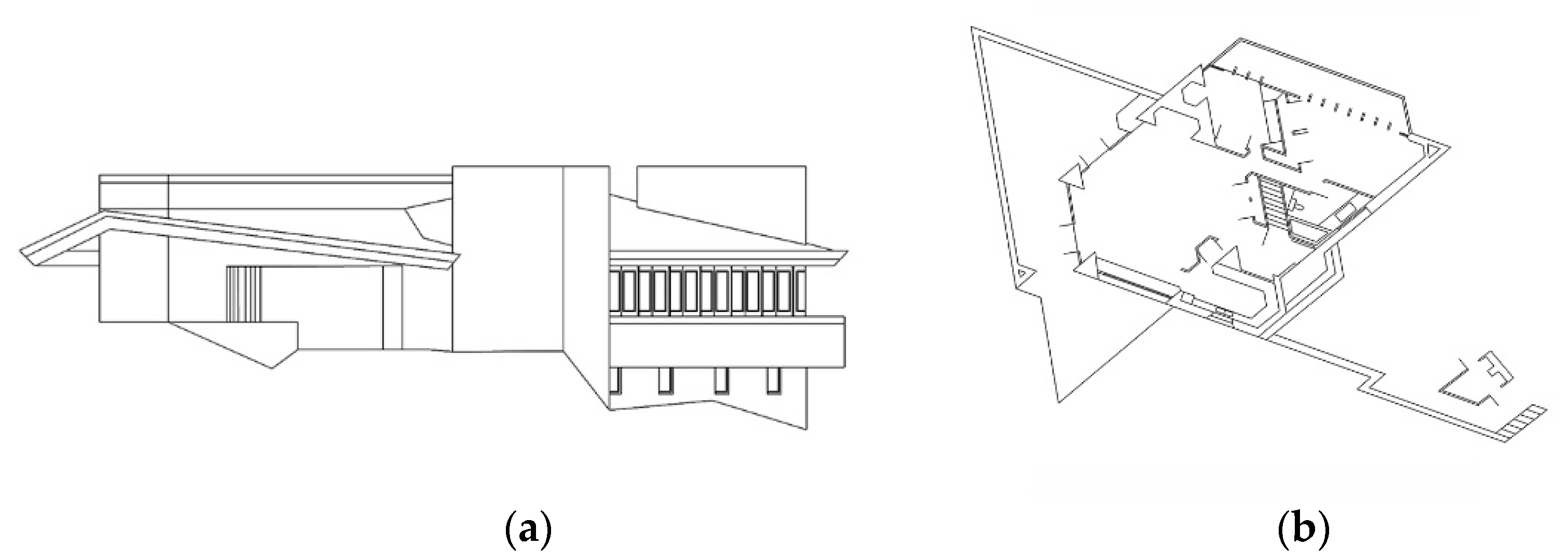
After completing Fallingwater, historians suggest that Wright moved in a different direction to create quintessentially American, suburban homes, which he named ‘Usonian’ works. Compared to Wright’s previous designs, the archetypal Usonian house had a simpler, non-ornamented design, delivering Wright’s unique sense of geometrical form (Figure 4). For Wright, the Usonian house was intended to embrace both natural elements and the natural philosophies of Jefferson and Ruskin, being truthful in their material expression. While there were multiple variations on the Usonian house, several were based on an underlying equilateral triangular planning grid known as ‘triangle-plan’ houses. Wright continued to design Usonian domestic buildings until his death.
Given these three clear stylistic periods in Wright’s career, it is not surprising that historians have questioned the place of Fallingwater in this body of work. Most commonly it has been suggested that Fallingwater differs from anything else Wright had designed. For example, Bernhard Hoesli contextualizes Fallingwater as ‘a mutation’, which ‘stands out as a unique achievement in [Wright’s…] career […] and it would also seem that in 1936 nothing in Frank Lloyd Wright’s previous work had prepared one to expect it.’ [13] (p. 204).
However, just because it has been argued that Fallingwater is a clear departure from Wright’s other domestic architectural styles does not mean that the position is universally accepted. For example, Kathryn Smith observes that while Fallingwater ‘has long been recognized as a unique building in [Wright’s] prodigious seventy-year career’ [14] (p. 1), she also notes that Fallingwater may not be as entirely unique in Wright’s repertoire. Smith suggests that ‘[t]he juxtaposition of building and waterfall was not new in Wright’s Kaufman House’ [14] (p. 1).
Laseau and Tice, despite acknowledging that Fallingwater is unique in many respects, also note that ‘[s]everal houses among Wright’s earlier work could provide plausible prototypes for Fallingwater’ [3] (p. 72). Robert McCarter [15] also identifies a selection of Wright’s previous designs which may have influenced Fallingwater and supports his argument with the following quote from Wright: ‘The ideas involved [in Fallingwater] are in no wise changed from those of early work. The materials and methods of construction come through them. The affects you see in this house are not superficial effects, and are entirely consistent with the prairie houses of 1901–10’ [15] (sic. p. 6). Such debates about the position of Fallingwater in Wright’s larger domestic canon can be found in many histories and scholarly critiques. Certainly, there are elements in Fallingwater that recall his previous designs, and which seem to prefigure his later Usonian works. As such, is Fallingwater a transition design, from the Textile-Block to the Usonian period, or was it a throwback to the Prairie style?
2.2. The Use of Fractal Analysis to Define Architectural Style
The concept of a fractal dimension (D), which was defined and popularized by Benoit Mandelbrot [16,17], is a mathematical measure of the relative diversity and density of geometric data in an image (where 1.0 < D < 2.0) or object (where 2.0 < D < 3.0). This property, which could also be thought of as ‘statistical roughness’ or ‘characteristic complexity’, is simply a measure of the volume and distribution of geometry in a form. From an architectural perspective, this property could be conceptualized as ‘the extent to which lines, regardless of their purpose, are both present in, and dispersed across, an elevation or plan’ [18].
In the case of the present research, the subjects of the fractal analysis are the physical forms and the visual details of buildings. One of the earliest attempts to calculate the fractal dimension of architecture using the box-counting method was undertaken by Carl Bovill [19], who measured the characteristic complexity of the elevations and plans of various canonical buildings. Since that time, fractal analysis (typically using variations of the box-counting method) has been used to calculate the formal properties of a growing number of buildings, ranging from ancient structures to twenty-first-century designs [20,21,22,23]. A stable computational version of the box-counting method for architectural analysis was first presented in 2008 [24] and it is now the accepted version in architectural scholarship as it is ‘easy to use and an appropriate method for measuring works of architecture with regard to continuity of roughness over a specific scale-range (coherence of scales)’ [25] (p. 703). However, researchers have also noted that the method has some weaknesses and have identified factors that can affect the accuracy of the result [20,24,26,27]. Solutions to these problems have since been identified [18]; the optimal settings for applying the box-counting method have been determined, and a defined approach to the method has been tested and refined by several scholars [18].
The raw numerical outputs for fractal analysis of buildings do not necessarily express anything meaningful until they are interpreted in the context of the building as an architectural form. Most publications that present fractal dimension results of architecture provide dimensions of building plans [21,28,29], elevations [22,23,30] and an overall dimension, combining values of the plans and elevations [5,18].
The fractal analysis of elevations typically focuses on depicting and measuring functional elements because the location of windows and doors and the modulation of walls, roofs, and balconies are all potentially expressions of function. In contrast, the fractal analysis of a building plan measures the formal complexity of a design, not as it can be seen in its totality, but as it can be experienced through movement or inhabitation [31]. While we can conceptually think of an elevation as being something that can be seen (with some correction for perspective) and therefore measured, an architectural plan view is largely invisible. For fractal analysis purposes, the plan view assumes that part of the building has been completely removed to reveal the interior spatial relationship that is experienced. In architectural research, the roof plan poses a different conceptual challenge as it could be regarded as ‘the fifth façade’ of the building, even though relatively few roof plans resemble their elevations so much as they resemble their internal plans [18,32]. For the purposes of fractal analysis, the roof plan is treated as a type of plan and is combined with other floor plans when calculating mean dimensions.
2.3. Fractal Analysis of Frank Lloyd Wright’s Buildings
Wright’s designs are probably the most common subject of fractal analysis in architecture [28,33,34]. An elevation of the Robie House (D = 1.520) was one of the earliest examples examined [20], and it has since generated a detailed response from other scholars [24,33,34,35]. Indeed, this one façade is probably the most frequently analysed of an example, with at least eight separate box-counting studies published. The results of these studies typically range from D = 1.520 [20] to D = 1.689 [36].
A total of twenty-one of Wright’s houses have been measured using the box-counting method. Wen and Kao [28] applied a computational version of the method to plans of five houses by Wright spanning from 1890 to 1937. The houses studied were the Frank Lloyd Wright House (D = 1.436), the Harley Brandley House (D = 1.626), the Avery Coonley House (D = 1.589), the Sherman M. Booth House (D = 1.609), and the Herbert Jacobs House (D = 1.477). Significantly, researchers have measured the fractal dimensions of the plans and elevations of fifteen houses by Wright across three stylistic periods [18].
Fractal analysis is used commonly in architectural research to provide quantitative comparisons between the formal properties of individual buildings [5,20,37,38] or the sets of buildings [18,28,39]. For example, it has been demonstrated that the fractal dimensions of Le Corbusier’s early works differ from those of his later works [29]. Likewise, fractal dimensions can be used to partially distinguish several distinct movements in architecture: Avant-Garde, Post-Modernism or Minimalism [18]. This past research demonstrates that using this method, it is possible to construct a comparison between different periods in Wright’s domestic designs and thereby determine where Fallingwater might fit into Wright’s body of work.
Past fractal dimension analysis of Prairie style and Usonian buildings in several publications has found a close range of results that supports the conventional interpretation of visually consistent buildings in these styles [5,40]. The published results for five of the Prairie-style houses constructed between 1901 and 1910 provide fractal dimensions for plans, elevation and composite results for the Henderson, Tomek, Evans, Zeigler and Robie houses. The findings show a level of uniformity in the mean, median and range results, with the range of fractal dimensions recorded between D = 1.4009 (Zeigler House) and D = 1.4738 (Evans House) [18]. The published results for five triangle-plan Usonian houses built between 1950 and 1955 provide fractal dimensions for plans, elevations and composite results for the Palmer, Dobkins, Reisley, Fawcett and Chahroudi Houses, with the results ranging between D = 1.350 (Fawcett House) and D = 1.486 (Palmer House) and the average for the set was D = 1.425 [18].
In contrast to the Prairie and Usonian houses, the five Textile-Block houses built between 1923 and 1929 are more diverse, being the only examples of a short-lived, almost experimental style. This is confirmed by fractal dimension trendlines for the Textile-Block houses, suggesting that these houses were an evolving process, rather than the steady-state results for the other two styles that had been refined over longer periods. The published results for the five Textile-Block houses constructed between 1923 and 1929 provide fractal dimensions for plans, elevation and composite results for the Millard, Storer, Samuel Freeman, Ennis and Richard Lloyd Jones houses with the results ranging between D = 1. 3660 (Millard House) and D = 1.5243 (Ennis House); the average for the set was D =1.4591 [18].
This past analysis of the visual complexity of 15 of Wright’s domestic designs shows that, despite some stylistic differences, there is a degree of visual consistency across each of Wright’s housing styles. For the mean elevation data, the Prairie and Textile-Block houses have an almost identical fractal dimension, and the Usonian result is only slightly lower. In his planning, Wright appears to have gone full-circle in terms of spatial complexity over time, starting from the Prairie style then increasing in the Textile-Block houses, before returning to the lower levels in the Usonian houses. Comparing the aggregate results of the three periods of Wright’s architecture, the Textile-Block buildings are generally the most complex, the Usonians are the least and the Prairie houses are midway between the two. The consistency in the appearance of Wright’s stylistic periods, especially the Usonian and Prairie styles—as proposed qualitatively and verified using fractal dimensions—implies that an unusual house such as Fallingwater might stand out among the others.
3. Method and Approach
3.1. The Box-Counting Method for Architecture
The box-counting method is well known in mathematics [17]. In its standard architectural application, there are four stages: (i) data preparation, (ii) data representation, (iii) pre-processing and (iv) processing. For the first of these stages, data preparation, computationally generated line drawings (CAD images) of plans and elevations are prepared, with all textures and natural features (shadows, vegetation and reflections) deleted. The content of the computational image is the subject of the second stage. That is, the researcher must decide which level of architectural information is required in the image. The first three standard representational levels are described as building outline, outline plus major changes in form, outline, changes in form and secondary modelling [18]. Most architectural analyses, and all of the works in the present paper, use level-four representation. Stage-three data pre-processing involves preparing the image for analysis using the thinnest line-weights and highest resolution images available to generate enough grid comparisons to produce a robust result. For the final stage, particular box-counting variables are determined, including the optimal scaling coefficient, being the ratio for successive grid comparisons, and the starting and closing grid size relative to the original image [18].
3.2. Approach
Two bodies of data are required for this paper: (1) fractal dimension measurements of Fallingwater, and (2) fractal dimension measurements of a representative sample of each of Wright’s three main stylistic periods.
- (1)
- The fractal dimensions of the elevations of Fallingwater are developed for the first time for this paper. The fractal dimensions of three floor plans and one roof plan of Fallingwater have been recently measured and published [41]. The plans were measured using the standard architectural box-counting method [18], and the elevations are also measured in the same way in this paper. In total, eight individual D results are developed from Fallingwater for comparative purposes.
- (2)
- The primary visual characteristics of Wright’s Prairie style are considered, as in past research, to be encapsulated in a set of five key works: Robie, Evans, Zeigler, Tomek and Henderson houses. For Wright’s Textile-Block style, the Ennis, Millard, Storrer, Freeman and Lloyd-Jones houses are, for all practical purposes, the complete set. For the Usonian works, the Palmer, Dobkins, Reisley, Fawcett and Chahroudi houses are considered representative of one type of Usonian planning. Fractal dimension measures for these 15 houses (58 elevations and 46 plans) were previously produced using the standard method [18].
The combination of new and previously published measures results in a data set (112 D results, and multiple derived results) sufficient to test claims about the position of Fallingwater in Wright’s larger body of work. This analysis is undertaken using graphs of trendlines, mean and aggregate results for different designs, and comparing their differences (range of D). The numerical results are then interpreted in combination with past scholarly arguments about Wright’s work, combining the quantitative and qualitative to produce a nuanced assessment of the data.
3.3. Derived Measures and Terminology
The results in this paper are reported using the standard architectural nomenclature for the results for plans, elevations and composite values. The ground floor plan is numbered zero (P0), and any floors above ground level are numbered consecutively from 1 (P1, P2, …) and the roof plan is labelled (PR). If one or more basement levels are present in a design, they are designated with negative integers (P−1, P−2, …). A measure of the typical level of formal complexity present in the spatial arrangement of the plan, and its corresponding exterior expression in the roof, is determined by calculating the mean of the DP# and DPR results for the house (μP). The elevations of each house are numbered (E1-4). A measure of the typical level of visual complexity observable in the exterior of the house is determined by calculating the mean DE value for the house (μE). To create a composite measure of the typical level of characteristic complexity present in the building, the DE1-4 and DP#-PR results for the house are combined into a mean for the entire house (μE+P). When the fractal dimension analysis expands from one building to a set of buildings the results are signified by the presence of curly brackets {…}. For a set of buildings, it is common to calculate mean results for all elevations (μ{E}), all plans (μ{P}) and a composite mean of all elevations and plans (μ{E+P}). Table 1 provides a summary of mathematical notations and definitions.
3.4. Interpretation of the Results
For interpreting the results, the ‘range’ (R), or difference between fractal dimensions, is typically calculated. R can be reported as a D value (D1 – D2 = DR) or more commonly as a percentage difference (because the fractal dimension of an image is between 1.0 and 2.0, it is easy to conceptualize as a percentage). R can be used to suggest how similar images or façades might appear in terms of their relative visual complexity. For the purpose of more intuitively understanding R results, Table 2 provides some indicative qualitative descriptors used in past research [18]. While these descriptors tend to overemphasize the strength of any similarities, they are still useful for comparing Fallingwater with other buildings by Wright.
For individual houses, the range within both plans and elevations is shown. For the stylistic sets, the range across the overall set is recorded. At the base of the comparative results table, the range between the highest and lowest composite results (combined plans and elevations for each house) are reported for the overall set.
4. Results
4.1. Full Set of Fractal Dimensions for Fallingwater
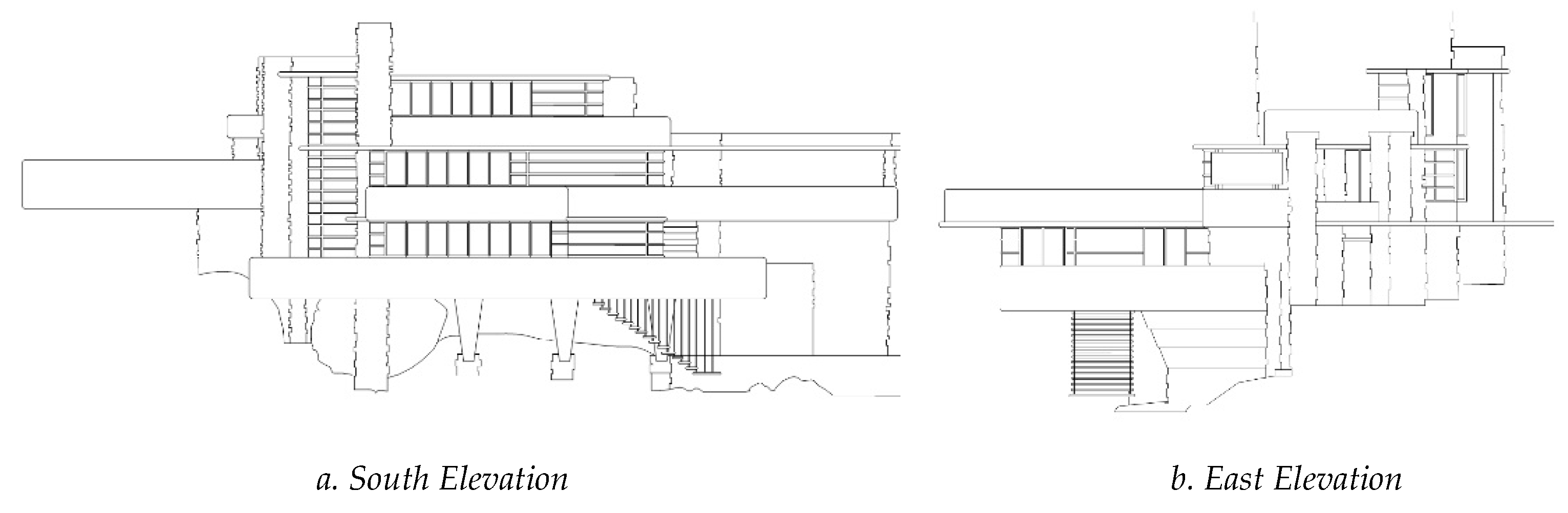
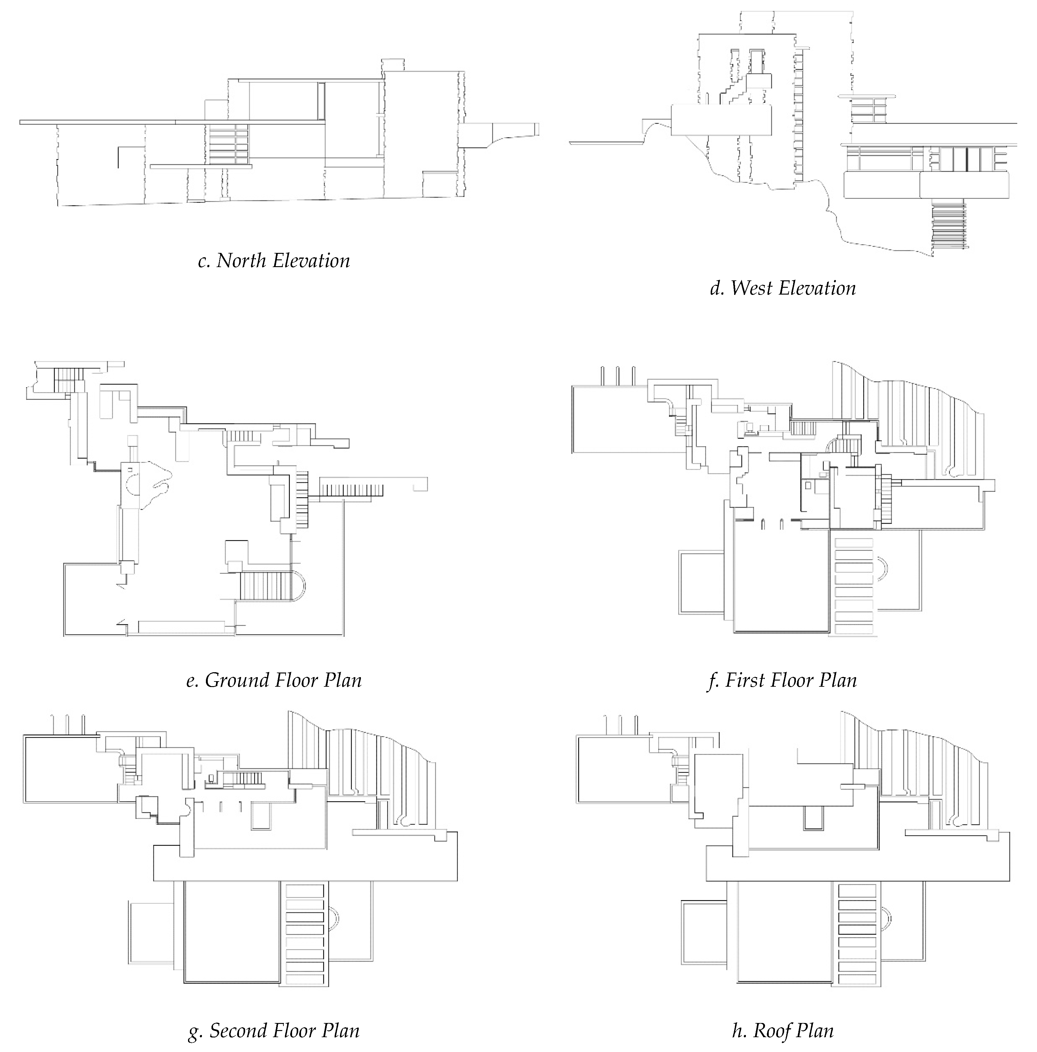
Figure 5 presents the source images for the fractal dimension calculations of Fallingwater and the measures derived from these images are reported in Table 3.
The fractal dimension results for the Fallingwater elevations indicate that the façade with the lowest result—or least amount of characteristic complexity—is the north (DE1 = 1.3321). This is the side facing the cliff and hill, without much outlook. In the northern hemisphere, the northern façade receives no direct sun, and as Wright designed houses to address the sun [42,43], it is no surprise that this elevation has less fenestration than the other façades, and correspondingly, less visual complexity. On the opposite side of the house is the south elevation, which features in most of the famous images of Fallingwater [2,6,44,45]. This south elevation is parallel to the Bear Run stream and it expresses much of the program of the house, with its layered balconies, their projecting roof overhangs, and the windows and doors that vary according to location and purpose. These details add up to a visually complex elevation and the results show it is the most geometrically expressive façade of the house (DE2 = 1.4628). The east elevation is the second most visually complex (DE3 = 1.4341), with the end view of the many stacked stone walls contributing to the visual complexity. Overall, these results contribute to the mean outcome for the elevations of the overall house (μE = 1.4019).
The floor plans of Fallingwater have a mean value of μP = 1.4085. Perhaps surprisingly, the ground floor plan—which contains the entry and living room and includes visually complex forms such as the existing boulder retained as the hearth for the fire and several stairways—has the lowest value (P0 = 1.3897). The greatest amount of formal information can be found on the first floor (P1 = 1.4439). In comparison to the open planning of the ground floor, this level features many rooms and passageways. This planning reflects the era, wealth and lifestyle of the Kaufmann family, with bedroom arrangements that appear unusual today. For example, this floor has one room each for the Kaufmanns, each with a personal bathroom, and a guest bedroom and another bathroom. The combination of these small rooms, several staircases and outdoor terraces increases the formal complexity of this plan.
While the roof plan of Fallingwater has the lowest complexity of the plans (PR = 1.3870) it is only slightly less complex than the second floor, in the order of R = 0.3%, an extremely small variation. Unlike many houses that have a simple roof covering the entire house—and a correspondingly low PR—Fallingwater’s cantilevering terraces, overhangs and outdoor staircases all add to the complexity of its roofscape. In particular, many of the living spaces of Fallingwater are outdoors, and these are captured in the roof plan, which shows all parts of the building down to the ground.
The range between the four elevations of Fallingwater is RE% = 13.07, which suggests they are, at best, in a qualitative sense, broadly comparable in terms of their visual properties. In contrast, the range of the plans of Fallingwater is RP% = 5.69, which suggests a higher degree of visual similarity. The mean of all plan and elevation results provides a composite indicator for the complete house (μE+P = 1.4052).
4.2. Initial Comparison Fallingwater to the Prairie, Textile-Block and Usonian Sets
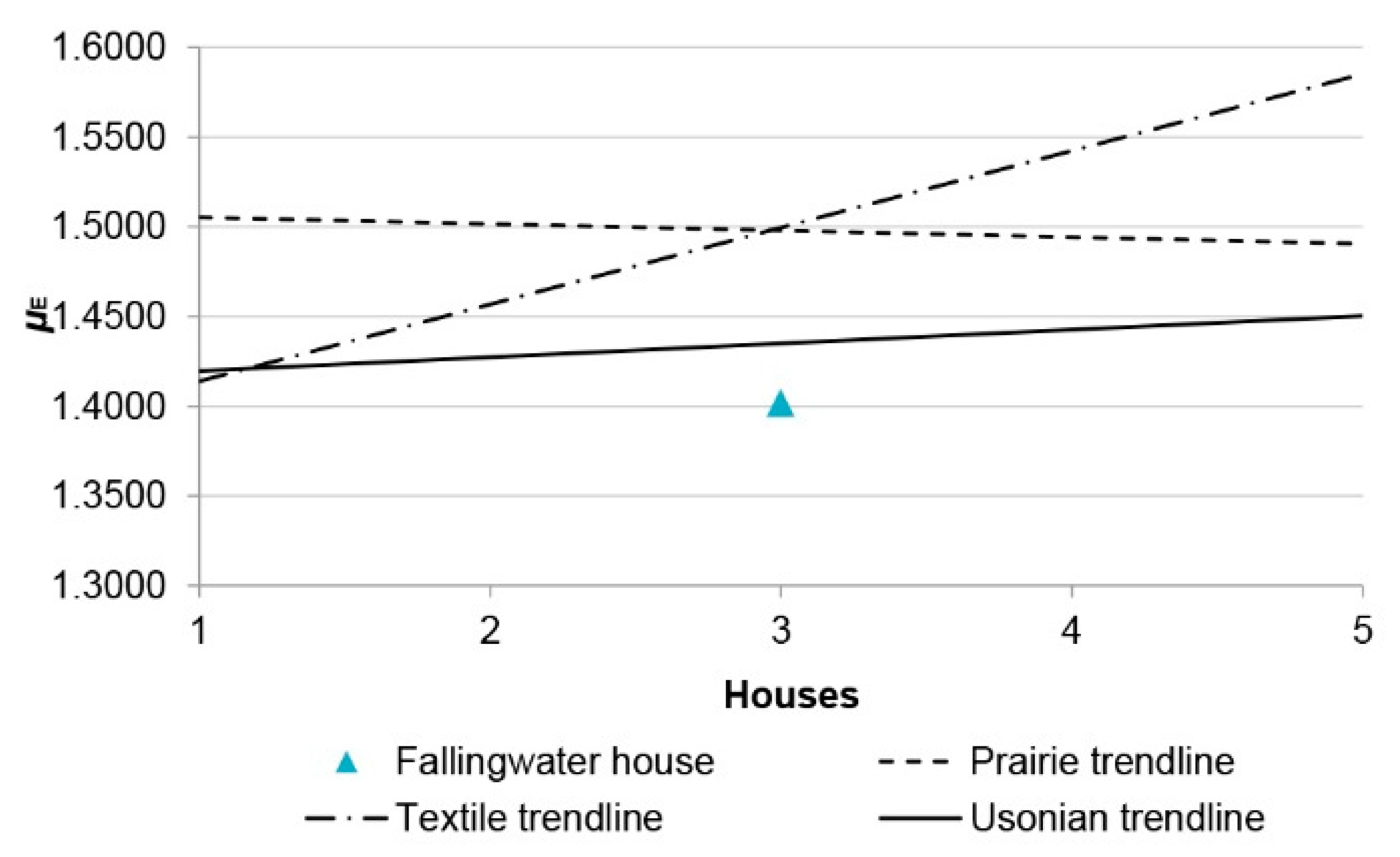
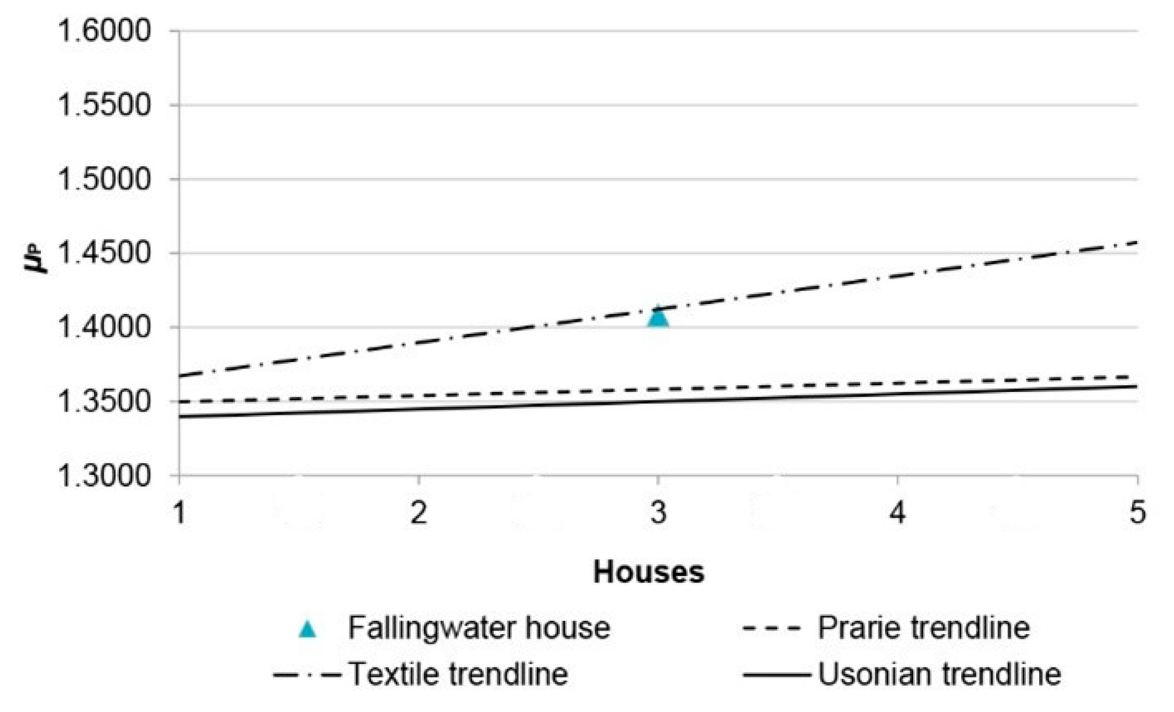
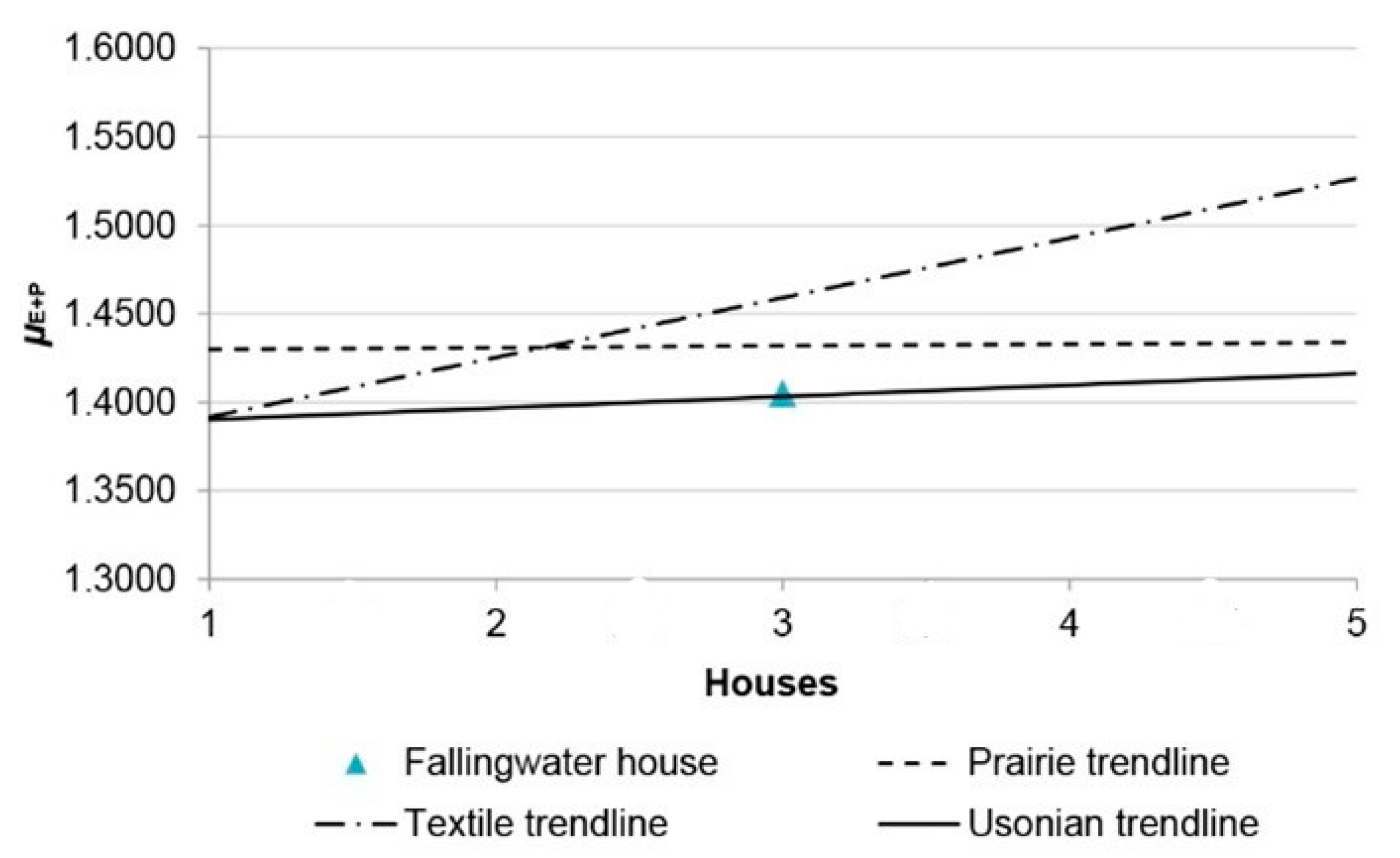
The full data tables for the 15 houses in the comparison are presented in the Appendix (Table A1, Table A2 and Table A3). There are multiple ways to compare the results for Fallingwater with those for the other houses. First, it must be acknowledged that while some of the formal properties of Wright’s three major styles are relatively consistent, others evolved over time. For example, just considering elevations, visual complexity is relatively constant across the works of Wright’s Prairie and Usonian houses, while it rises over time in his Textile-Block houses (Figure 6, Table 4). For the plans, the same pattern occurs, with the Prairie and Usonian houses remaining similar in their complexity and the Textile-Block houses increasing over time (Figure 7, Table 5). Finally, when elevations and plans are combined, these trends are crystalized, with the Prairie houses remaining extremely stable, the Usonian houses increase in complexity slightly over time and there is a dramatic increase in the results for the Textile-Block houses. (Figure 8, Table 6). In each of these figures, the equivalent mean fractal dimension result for Fallingwater is included.
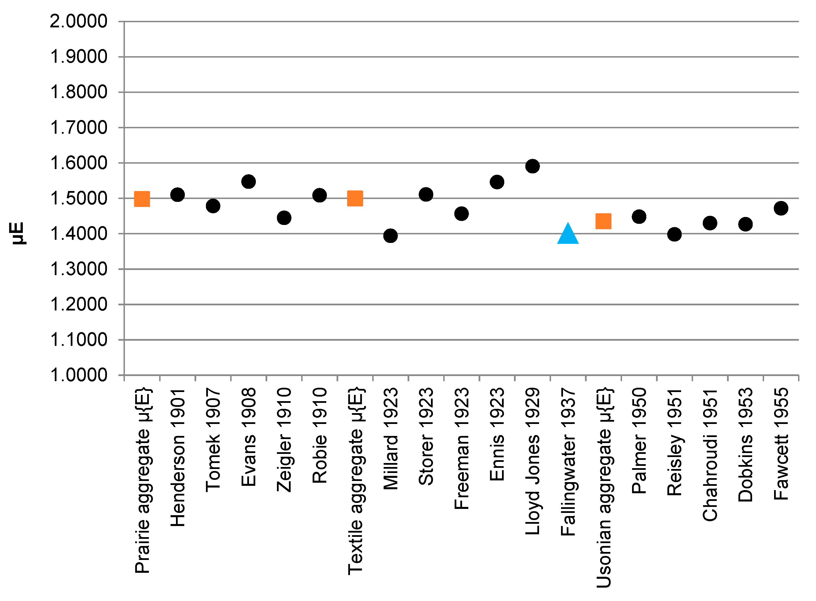
When the mean results for each house and for each set (‘aggregate’) are graphed, the results show Fallingwater generally has lower levels of formal complexity than most of the other houses measured, although it is never the least visually complex. Considering the elevation results, only two of the 15 houses have a lower overall visual complexity in elevation—the Textile-Block Millard House (μE = 1.3942) and the Usonian Reisley House (μE = 1.3982)—than Fallingwater (μE = 1.4019) (Figure 9). The aggregate values for the elevations of each set (μ{E}) show that compared to the stylistic periods, Fallingwater has the least complex elevations, followed by the Usonian houses, then the Prairie style, which is only slightly less complex than the Textile-Block elevations.
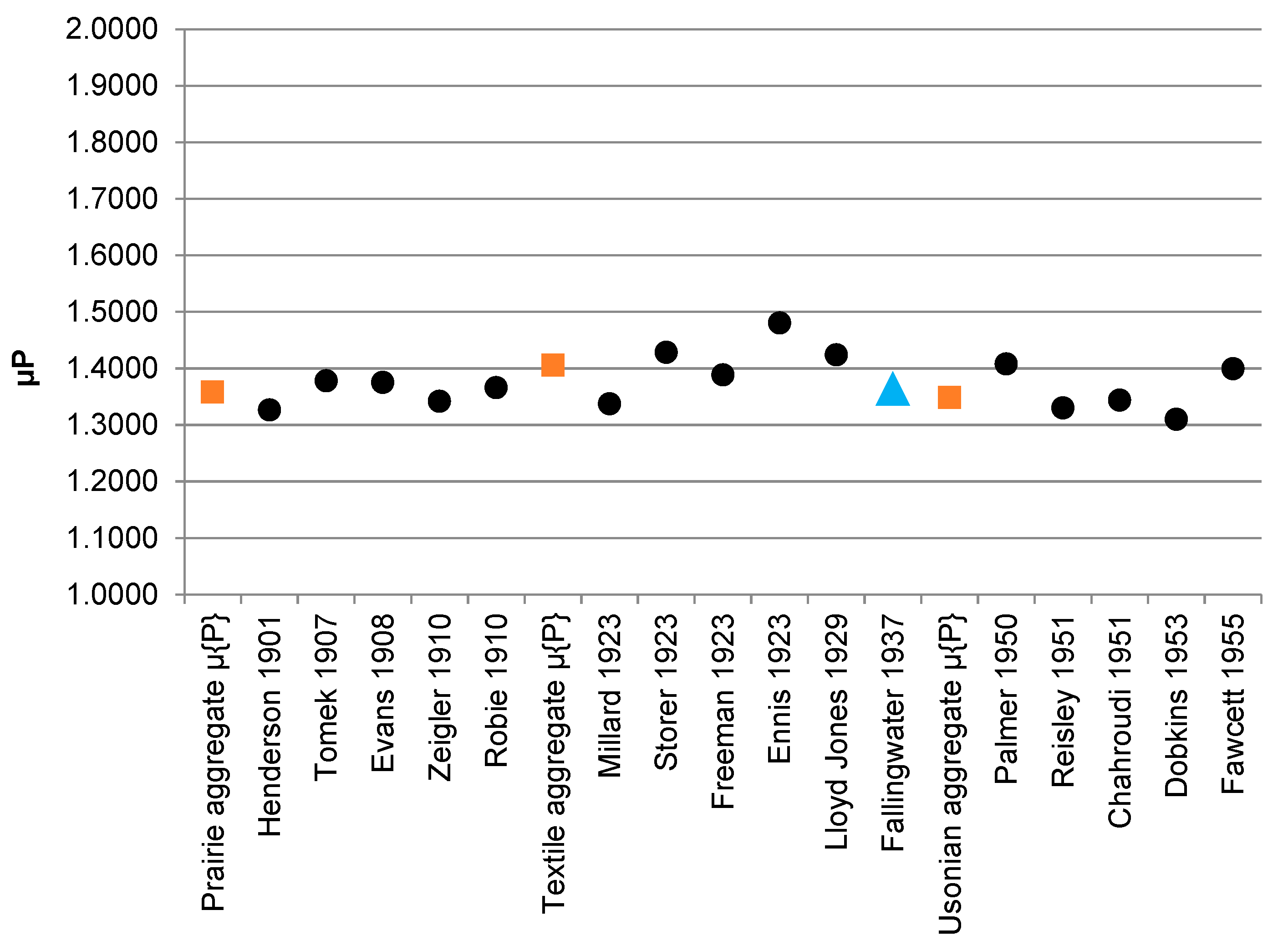
In plan form, Fallingwater’s mean dimension (μP = 1.4085) is more typical in the data, with just over one-third of the houses having lower complexity than Fallingwater (Figure 10). These include the Millard House and the Reisley House (which also had lower elevation results) and two other Prairie and two other Usonian style houses. In the aggregates of the stylistic sets, compared with the mean values for Fallingwater, the plans (μ{P}) for the Usonian and Prairie styles are only just less complex than Fallingwater, while the Textile-Block plans have higher fractal dimensions (Figure 11).
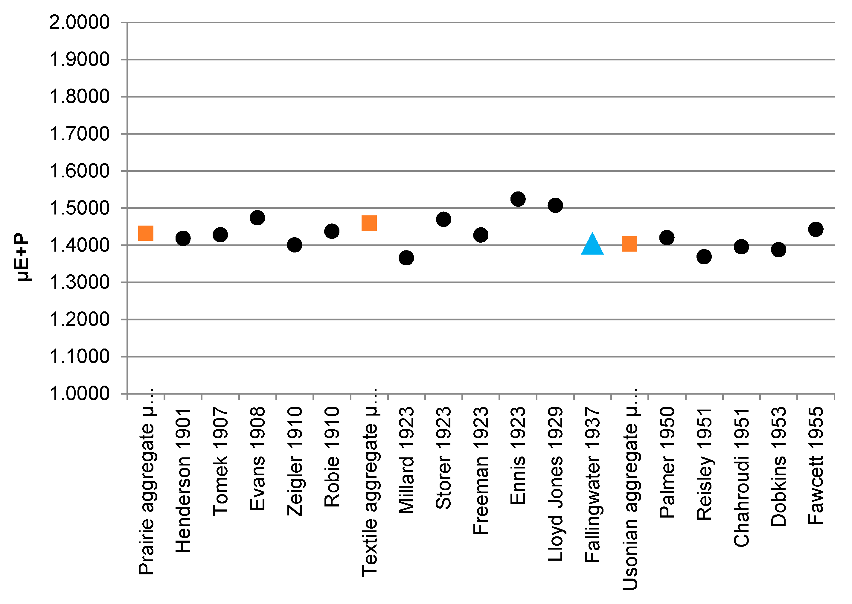
In summary, the elevations of Fallingwater have some broad visual similarities to two of the 15 houses, and when trendlines and aggregate dimensions are considered, they are closest to the properties of the Usonian houses. In contrast, the plans of Fallingwater are generally more complex than both the Usonian works and the Prairie style works. When considering trendlines and aggregate results, the plans of Textile-Block houses are closest to the results for Fallingwater, but this is not supported at a finer level. The individual results confirm that four of the five Textile-Block houses have greater complexity in plan than Fallingwater. The composite results position the visual properties of Fallingwater closest to those of the Usonian houses.
4.3. Detailed Comparison Fallingwater to the Prairie, Textile-Block and Usonian Sets
The mean results for all houses are compared in Table 7. The R values in the table are set using Fallingwater as a target value, and the R% values provided are the difference between the μ value for the house and the μ value for Fallingwater. Thus, the Rμ indicates the percentage by which the houses differ from Fallingwater, in elevation (RμE%), plan (RμP%), and their composite value (RμE+P%).
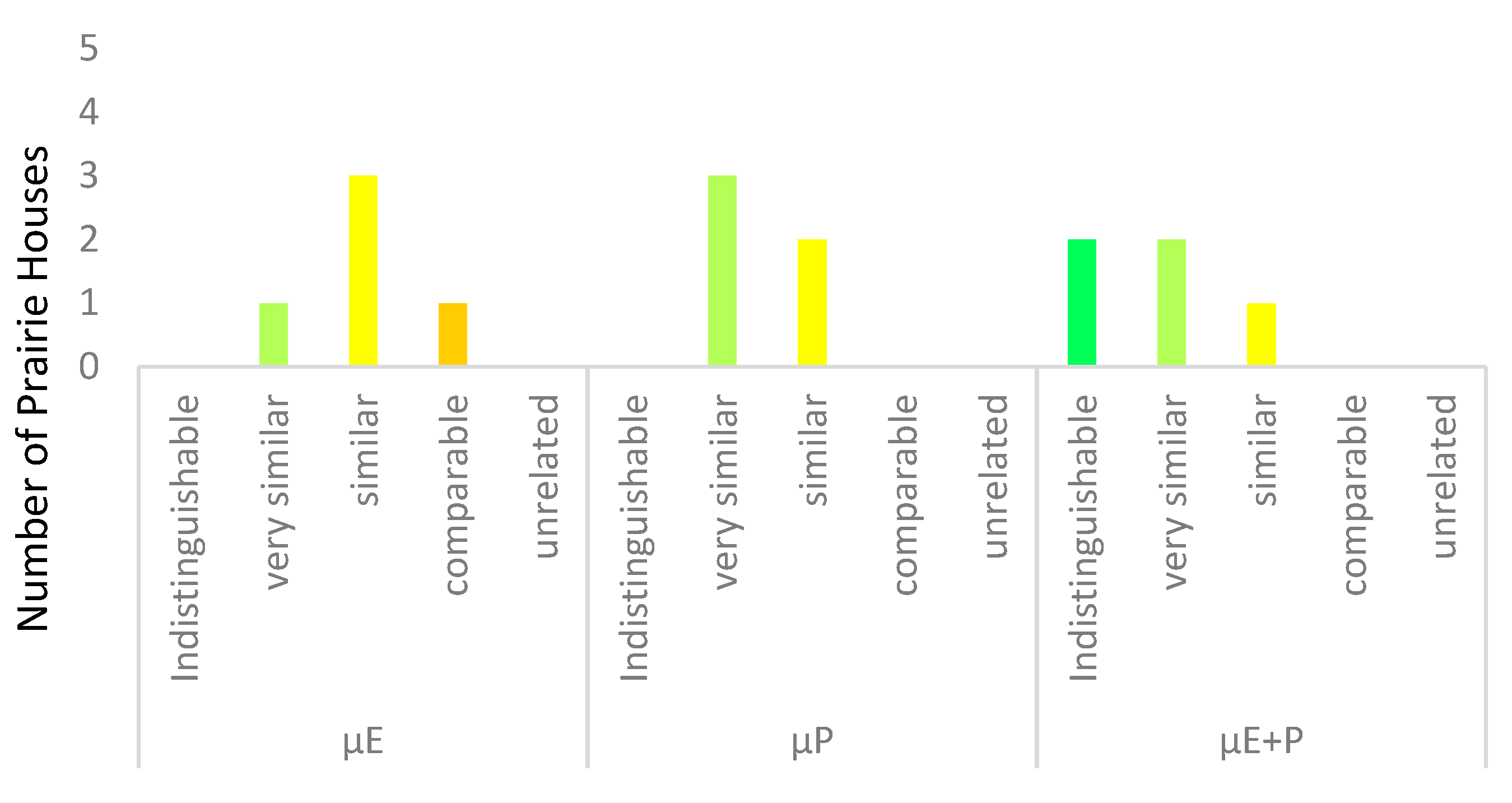
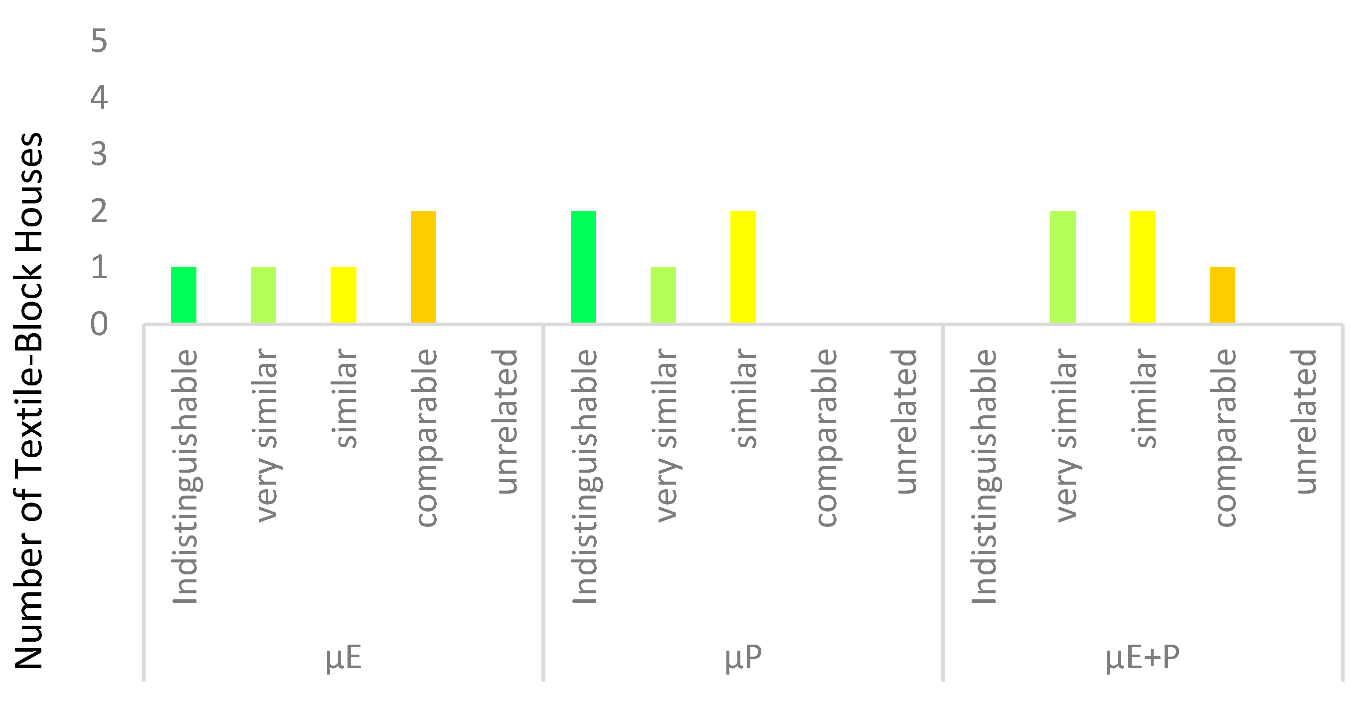
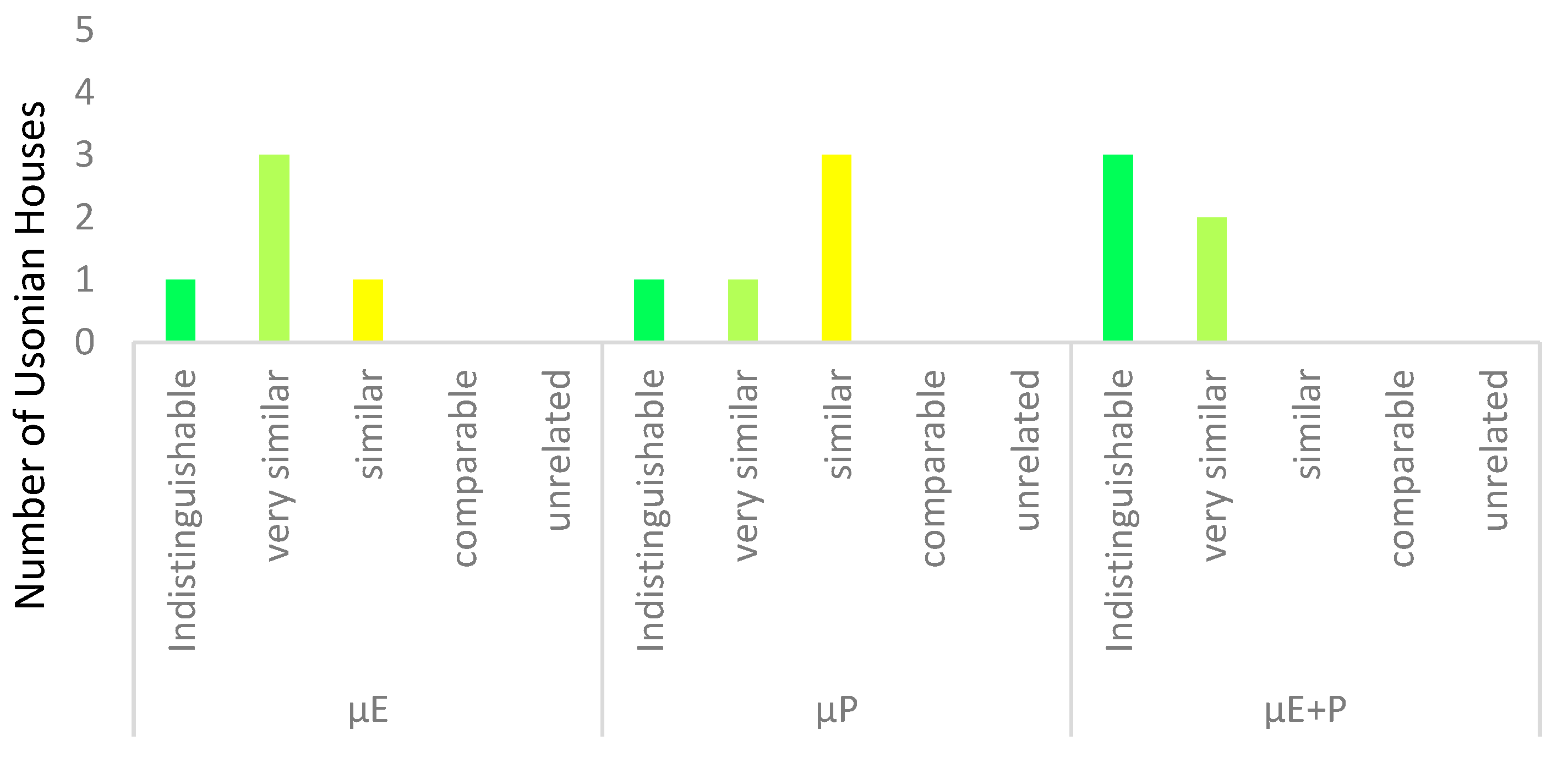
Figure 12, Figure 13 and Figure 14 compare the difference of the houses to Fallingwater, using a qualitative interpretation of results. These figures present the mean data in elevation (μE), plan (μP), and in combination (μE+P), where the x-axis is generated with reference to the qualitative descriptors used for ranges provided in Table 2. The terms in the x-axis describe how similar or different individual houses are to Fallingwater, and the columns increase in the y-axis depending on the number of houses with that level of visual similarity. To clarify that these terms are derived from the table, and they are mentioned in the descriptions that follow the charts in inverted commas.
Overall, the five Prairie-style houses are typically ‘similar’, or ‘very similar’ to Fallingwater in plan and elevation, and while the composite means of two of the Prairie houses are ‘indistinguishable’, no aspects of the houses are ‘unrelated’ to Fallingwater. The composite of the elevation and plans for the Zeigler House could be considered ‘indistinguishable’ in comparison to Fallingwater (RμE+P% = 0.4343), and this is the lowest composite RμE+P% for all 15 houses. Within the Prairie style set, the Zeigler House is the closest set of elevations set to Fallingwater (RμE% = 4.2925) and the Tomek House has the closest set of plans (RμP% = 2.9800), but is less like Fallingwater in elevation (RμE% = 7.3625).
There is no clear relationship or clustering of the results for the Textile-Block houses and Fallingwater. While the Millard House is the only house ‘indistinguishable’ from Fallingwater in elevation (RμE% = 0.7700), and the Lloyd-Jones House (RμP% = 1.5950) and the Freeman House (RμP% = 1.9700) are ‘indistinguishable’ in the plan, none of these results suggest a house that is so alike when the composite values are considered. Overall, the results suggest the plans of the Textile-Block houses are the most comparable to Fallingwater.
The Usonian set is the most related to Fallingwater in terms of their visual complexity. Unlike the other two styles, none of the houses in the Usonian set are either ‘comparable’ or ‘unrelated’ to Fallingwater. Three of the houses are effectively ‘indistinguishable’ in their composite result, the Chahroudi House being the closest to Fallingwater for this set (RμE+P% = 0.9540). Two of the Usonian houses have the least difference to Fallingwater of all the fifteen houses tested; the Reisley House elevations are ‘indistinguishable’ to those of Fallingwater (RμE% = 0.3750) and the Fawcett House is ‘very similar’ in plan (RμP% = 0.8800), more so than any of the other 14 houses.
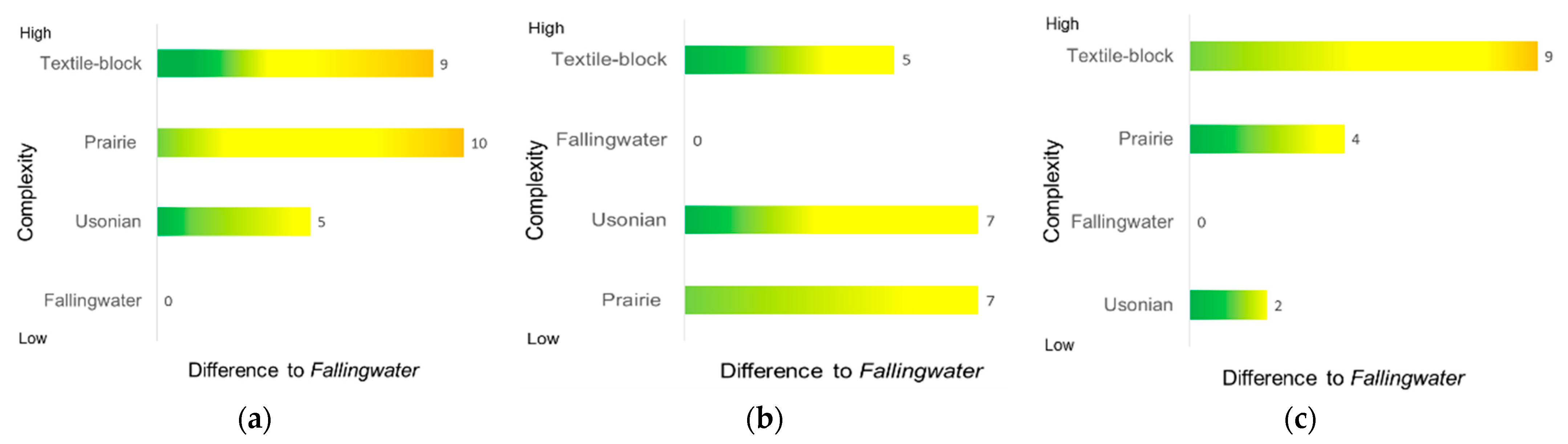
From the data presented in this section and the previous one, a profile is generated of Fallingwater in comparison to Wright’s other houses under study (Figure 15). This shows the complexity of the styles and of Fallingwater ranked according to mean D on the y–axis and then a bar indicating the mean range of each style from Fallingwater along the x–axis. This bar graph is determined by loading the occasions of ‘indistinguishable’ to ‘unrelated’ (extracted from Table 2) with numerical weight from 0–4. ‘Indistinguishable’ suggests little difference from Fallingwater (0)—the lower the result, the shorter the bar, and the more similar the style could be described as being to Fallingwater.
5. Conclusions
In general, and contrary to the arguments of scholars such as Lind, Pfeiffer and Hoesli, Wright’s Fallingwater has a level of formal complexity that is broadly akin to his other architectural styles. Certainly, when compared to elevations of other houses by Wright, Fallingwater’s elevations generally have a lower level of formal complexity than most of the other houses measured. Despite this general observation, Fallingwater’s elevations are similar to a few Usonian houses in terms of characteristic complexity. In plan form, Fallingwater typically has a similar level of complexity to the majority of the other houses. For the mean plan results, Fallingwater has a higher level of formal complexity than the Usonian and Prairie houses, and it shares a similar level of complexity to the Textile-Block homes. When these results are combined as a composite of plan and elevation, only the Usonian style is less complex than Fallingwater, but it is also the most similar. Thus, within the limits of the method, the results indicate that the visual complexity of Fallingwater is not atypical of Wright’s Prairie, Textile-Block and Usonian houses and indeed, in terms of formal expression, it is broadly similar to the last group.
This finding has several practical limitations which must be taken into account when interpreting the result. First, while this paper adopts the same data sets used in previous research to represent Wright’s Prairie, Textile-Block and Usonian style works, only the middle set, the Textile-Block, could be said to capture the complete group of works produced in this style. For the other two, major works were chosen, but many more examples could equally be measured, producing slightly divergent results. Second, this paper measures the level and distribution of formal information in architectural images, which is just one aspect of architectural character. As such, when historians argue that Fallingwater is dissimilar in character to Wright’s other works, they are also taking into account aspects of the designs that are not measured in this paper. Such properties could include color, texture, and the phenomenological presence of the building on its site.
Finally, previous research [18] has shown that while D calculations for elevations often result in relatively consistent patterns across sets of an architect’s works, results for plans can be less consistent. This occurs because D results for plans are heavily influenced by a building ‘program’ (the number of bedrooms, the inclusion of specialist spaces like libraries or music rooms or servant’s quarters), as well as construction methods and social values of the era in which it was built (open plan vs. compartmentalized plan). As such, when considering works produced by Wright over a 54-year timeframe, there are potentially more factors shaping, or confounding, the D results for plans. A larger study with data normalized by program size or era would be needed to investigate this particular issue in more detail.
Author Contributions
Conceptualization, J.V. and M.J.O.; methodology, J.V. and M.J.O.; validation, J.V. and M.J.O.; formal analysis, J.V. and M.J.O.; investigation J.V. and M.J.O. writing—original draft by J.V.; writing—review and editing by M.J.O. All authors have read and agreed to the published version of the manuscript.
Funding
This research received no external funding.
Data Availability Statement
All the data used in this study are available in the paper and in Appendix A.
Conflicts of Interest
The authors declare no conflict of interest.
Appendix A

Table A1.
Prairie set results.
| Houses | Henderson | Tomek | Evans | Zeigler | Robie | Set {…} | |
|---|---|---|---|---|---|---|---|
| Elevations | DE1 | 1.5255 | 1.5103 | 1.5592 | 1.4442 | 1.5174 | |
| DE2 | 1.5177 | 1.4885 | 1.5709 | 1.4542 | 1.5708 | ||
| DE3 | 1.4910 | 1.4342 | 1.5254 | 1.4385 | 1.4785 | ||
| DE4 | 1.5072 | 1.4799 | 1.5337 | 1.4424 | 1.4677 | ||
| μE | 1.5104 | 1.4782 | 1.5473 | 1.4448 | 1.5086 | ||
| μ{E} | 1.4979 | ||||||
| M{E} | 1.4991 | ||||||
| std{E} | 0.0432 | ||||||
| Plans | DP-1 | 1.3001 | 1.4448 | ||||
| DP0 | 1.4499 | 1.3902 | 1.4307 | 1.4170 | 1.3385 | ||
| DP1 | 1.3763 | 1.3721 | 1.3817 | 1.3802 | 1.4220 | ||
| DP2 | - | - | - | - | 1.3984 | ||
| DPR | 1.1817 | 1.3077 | 1.3147 | 1.2295 | 1.3066 | ||
| μP | 1.3270 | 1.3787 | 1.3757 | 1.3422 | 1.3664 | ||
| μ{P} | 1.3579 | ||||||
| M{P} | 1.3783 | ||||||
| std{P} | 0.0734 | ||||||
| Composite | μE+P | 1.4187 | 1.4285 | 1.4738 | 1.4009 | 1.4375 | |
| Aggregate | μ{E+P} | 1.4318 |
Note: “-“ means no result—there is no floor plan at this level to analyse.
Table A2.
Textile-Block set results.
| Houses | Millard | Storer | Freeman | Ennis | Lloyd-Jones | Set{…} | |
| Elevations | DE1 | 1.4420 | 1.5389 | 1.3603 | 1.6130 | 1.5947 | |
| DE2 | 1.4786 | 1.5543 | 1.5125 | 1.6390 | 1.5589 | ||
| DE3 | 1.3434 | 1.5111 | 1.4666 | 1.4900 | 1.6105 | ||
| DE4 | 1.3128 | 1.4395 | 1.4868 | 1.4417 | 1.5983 | ||
| μE | 1.3942 | 1.5110 | 1.4566 | 1.5459 | 1.5906 | ||
| μ{E} | 1.4996 | ||||||
| M{E} | 1.5006 | ||||||
| std{E} | 0.0925 | ||||||
| Plans | DP0 | 1.4078 | 1.4497 | 1.3964 | 1.4955 | 1.4465 | |
| DP1 | 1.3801 | 1.4330 | 1.3799 | - | 1.4228 | ||
| DP2 | 1.2826 | 1.4311 | - | - | 1.4158 | ||
| DPR | 1.2809 | 1.4024 | 1.3901 | 1.4664 | 1.4127 | ||
| μP | 1.3379 | 1.4291 | 1.3888 | 1.4810 | 1.4245 | ||
| μ{P} | 1.4055 | ||||||
| M{P} | 1.4127 | ||||||
| std{P} | 0.0557 | ||||||
| Composite | μE+P | 1.3660 | 1.4700 | 1.4275 | 1.5243 | 1.5075 | |
| Aggregate | μ{E+P} | 1.4591 |
Note: “-“ means no result—there is no floor plan at this level to analyse.
Table A3.
Usonian set, results.
| Houses | Palmer | Reisley | Chahroudi | Dobkins | Fawcett | Set {…} | |
|---|---|---|---|---|---|---|---|
| Elevations | DE1 | 1.4802 | 1.3865 | 1.4328 | 1.4596 | 1.3991 | |
| DE2 | 1.4461 | 1.3710 | 1.4529 | 1.3375 | 1.5575 | ||
| DE3 | 1.4642 | 1.4086 | - | 1.5359 | - | ||
| DE4 | 1.4018 | 1.4265 | 1.4045 | 1.3745 | 1.4591 | ||
| μE | 1.4481 | 1.3982 | 1.4301 | 1.4269 | 1.4719 | ||
| μ{E} | 1.4350 | ||||||
| M{E} | 1.4297 | ||||||
| std{E} | 0.0560 | ||||||
| Plans | DP-1 | - | 1.2968 | - | - | - | |
| DP0 | 1.4412 | 1.3687 | 1.3973 | 1.3810 | 1.4155 | ||
| DPR | 1.2875 | 1.3256 | 1.2908 | 1.2400 | 1.3839 | ||
| μP | 1.3644 | 1.3304 | 1.3441 | 1.3105 | 1.3997 | ||
| μ{P} | 1.3480 | ||||||
| M{P} | 1.3687 | ||||||
| std{P} | 0.0634 | ||||||
| Composite | μE+P | 1.4202 | 1.3691 | 1.3957 | 1.3881 | 1.4430 | |
| Aggregate | μ{E+P} | 1.4032 |
Note: “-“ means no result—there is no floor plan at this level to analyse.
References
- Alofsin, A. Frank Lloyd Wright and Modernism. In Frank Lloyd Wright, Architect; Riley, T., Alofsin, A., Eds.; Museum of Modern Art (New York) and Frank Lloyd Wright Foundation: New York, NY, USA, 1994; pp. 32–57. [Google Scholar]
- Pfeiffer, B.B. Frank Lloyd Wright, 1867–1959: Building for Democracy; Taschen: Köln, Germany, 2004. [Google Scholar]
- Laseau, P.; Tice, J. Frank Lloyd Wright: Between Principle and Form; Van Nostrand Reinhold: New York, NY, USA, 1992. [Google Scholar]
- Koning, H.; Eizenberg, J. The language of the prairie: Frank Lloyd Wright’s prairie houses. Environ. Plan. B Plan. Des. 1981, 8, 295–323. [Google Scholar] [CrossRef]
- Vaughan, J.; Ostwald, M.J. The relationship between the fractal dimension of plans and elevations in the architecture of Frank Lloyd Wright: Comparing the Prairie style, Textile-block and Usonian periods. ArS Archit. Sci. 2011, 4, 21–44. [Google Scholar]
- Kaufmann, E. Fallingwater, a Frank Lloyd Wright Country House; Abbeville Press: New York, NY, USA, 1986. [Google Scholar]
- McCarter, R. Frank Lloyd Wright; Phaidon: London, UK, 1999. [Google Scholar]
- Storrer, W.A. The Frank Lloyd Wright Companion; University of Chicago Press: Chicago, IL, USA, 2006. [Google Scholar]
- Green, A.G. Organic architecture: The principles of Frank Lloyd Wright. In Frank Lloyd Wright in the Realm of Ideas; Nordland, G., Pfeiffer, B.B., Eds.; Southern Illinois University Press: Carbondale, IL, USA, 1988; pp. 133–142. [Google Scholar]
- Maddex, D. 50 Favourite Rooms by Frank Lloyd Wright; Thames & Hudson: London, UK, 1998. [Google Scholar]
- Lind, C. Frank Lloyd Wright’s Fallingwater; Pomegranate: San Francisco, CA, USA, 1996. [Google Scholar]
- Futagawa, Y.; Pfeiffer, B.B. Fallingwater; A.D.A: Tokyo, Japan, 2009. [Google Scholar]
- Hoesli, B. From the Prairie house to Fallingwater. In On and by Frank Lloyd Wright: A Primer of Architectural Principles; McCarter, R., Ed.; Phaidon: London, UK, 2005; pp. 204–215. [Google Scholar]
- Smith, K. A beat of the rhythmic clock of nature: Frank Lloyd Wright’s waterfall buildings. In Wright Studies, Volume Two: Fallingwater and Pittsburgh; Menocal, N.G., Ed.; Southern Illinois University Press: Carbondale, IL, USA, 2000; pp. 1–31. [Google Scholar]
- McCarter, R. Fallingwater; Phaidon: London, UK, 2002. [Google Scholar]
- Mandelbrot, B.B. The Fractal Geometry of Nature; W.H. Freeman: New York, NY, USA, 1977. [Google Scholar]
- Mandelbrot, B.B. The Fractal Geometry of Nature. Updated and Augmented; Freeman: San Francisco, CA, USA, 1982. [Google Scholar]
- Ostwald, M.J.; Vaughan, J. The Fractal Dimension of Architecture; Springer International Publishing: Basel, Switzerland, 2016. [Google Scholar]
- Bovill, C. Fractal Geometry in Architecture and Design; Design Science Collection; Birkhäuser: Boston, MA, USA, 1996. [Google Scholar]
- Burkle-Elizondo, G. Fractal geometry in Mesoamerica. Symmetry Cult. Sci. 2001, 12, 201–214. [Google Scholar]
- Rian, I.M.; Park, J.H.; Hyung, U.A.; Chang, D. Fractal geometry as the synthesis of Hindu cosmology in Kandariya Mahadev temple, Khajuraho. Build. Environ. 2007, 42, 4093–4107. [Google Scholar] [CrossRef]
- Lionar, M.L.; Ediz, Ö. Measuring Visual Complexity of Sedad Eldem’s SSK Complex and Its Historical Context: A Comparative Analysis Using Fractal Dimensions. Nexus Netw. J. 2020, 22, 701–715. [Google Scholar] [CrossRef]
- Vaughan, J.; Ostwald, M.J. Measuring the significance of façade transparency in Australian regionalist architecture: A computational analysis of 10 designs by Glenn Murcutt. Archit. Sci. Rev. 2014, 57, 249–259. [Google Scholar] [CrossRef]
- Ostwald, M.J.; Vaughan, J.; Tucker, C. Characteristic visual complexity: Fractal dimensions in the architecture of Frank Lloyd Wright and Le Corbusier. In Nexus VII: Architecture and Mathematics; Kim Williams Books: Turin, Italy, 2008; pp. 217–231. [Google Scholar]
- Lorenz, W.E. Fractal geometry of architecture: Implementation of the box-counting method in a CAD-software. In Computation: The New Realm of Architectural Design, Proceedings of the 27th eCAADe Conference on Education and Research in Computer Aided Design in Europe, Istanbul, Turkey, 16–19 September 2009; eCAADe: Istanbul, Turkey; pp. 697–704.
- Benguigui, L.; Czamanski, D.; Marinov, M.; Portugali, Y. When and where is a city fractal? Environ. Plan. B Plan. Des. 2000, 27, 507–519. [Google Scholar] [CrossRef] [Green Version]
- Lorenz, W. Estimating the fractal dimension of architecture: Using two measurement methods implemented in AutoCAD by VBA. In Digital Physicality—Proceedings of the 30th eCAADe Conference, Czech Technical University in Prague, Prague, Czech Republic, 12–14 September 2012; Achten, H., Pavlicak, J., Hulin, J., Matejdan, D., Eds.; eCAADe and CVUT: Prague, Czech Republic; pp. 505–513.
- Wen, K.C.; Yu-Neng, K. An analytic study of architectural design style by fractal dimension method. In Proceedings of the 22nd ISARC, Ferrara, Italy, 11–14 September 2005; pp. 1–6. [Google Scholar]
- Vaughan, J.; Ostwald, M.J. A quantitative comparison between the formal complexity of Le Corbusier’s Pre-Modern (1905–1912) and Early Modern (1922-1928) architecture. Des. Princ. Pract. Int. J. 2009, 3, 359–372. [Google Scholar] [CrossRef]
- Samper, A.; Herrera, B. The fractal pattern of the French Gothic cathedrals. Nexus Netw. J. 2014, 16, 251–271. [Google Scholar] [CrossRef] [Green Version]
- Ostwald, M.J. Examining the relationship between topology and geometry: A configurational analysis of the rural houses (1984– 2005) of Glenn Murcutt. J. Space Syntax. 2011, 2, 223–246. [Google Scholar]
- Leupen, B.; Grafe, C.; Körnig, N.; Lamp, M.; de Zeeuw, P. Design and Analysis; Van Nostrand Reinhold: New York, NY, USA, 1997. [Google Scholar]
- Sala, N. Fractal models in architecture: A case of study. In Proceedings of the International Conference on Mathematics Education into the 21st Century: Mathematics for Living, The Third World Forum, Amman, Jordan, 18–23 November 2000; Rogerson, A., Ed.; The Mathematics Education into the 21st Century Project and The Third World Forum. [Google Scholar]
- Lorenz, W. Fractals and Fractal Architecture. Master’s Dissertation, Vienna University of Technology, Vienna, Austria, 2003. [Google Scholar]
- Ma, L.; Zhang, H.; Lu, M. Building’s Fractal Dimension Trend and Its Application in Visual Complexity Map. Build. Environ. 2020, 178, 106925. [Google Scholar] [CrossRef]
- Vaughan, J.; Ostwald, M.J. Using fractal analysis to compare the characteristic complexity of nature and architecture: Re-examining the evidence. Archit. Sci. Rev. 2010, 53, 323–332. [Google Scholar] [CrossRef]
- Lorenz, W. Complexity across scales in the work of Le Corbusier Using box-counting as a method for analysing facades. In Proceedings of the CAADENCE in Architecture 2016, Budapest University of Technology and Economics, Budapest, Hungary, 16–17 June 2016. [Google Scholar]
- Ostwald, M.J.; Vaughan, J. Calculating Visual Complexity in Peter Eisenman’s Architecture. In CAADRIA 2009: Between Man and Machine Integration/Intuition/Intelligence; Chang, T.-W., Champion, E., Chien, S.-F., Eds.; National Yunlin University of Science & Technology Department of Digital Media Design: Yunlin, Taiwan, 2009; pp. 75–84. [Google Scholar]
- Ohuchi, H.; Kimura, T.; Zong, S.; Kanai, S.; Kuroiwa, T. Quantitative Evaluation of Architectural Style Using Image Correlation and Fractal Dimension Analysis in Agora of Ancient Greek City Athens. AST 2020, 103, 37–45. [Google Scholar]
- Ostwald, M.J.; Vaughan, J. The mathematics of style in the architecture of Frank Lloyd Wright: A computational, fractal analysis of formal complexity in fifteen domestic designs. In Built Environment: Design Management and Applications; Geller, P.S., Ed.; NOVA Science Publishers: Hauppauge, NY, USA, 2010; pp. 63–88. [Google Scholar]
- Vaughan, J.; Ostwald, M.J. Measuring the geometry of nature and architecture: Comparing the visual properties of Frank Lloyd Wright’s Fallingwater and its natural setting. Open House Int. 2022, 47, 51–67. [Google Scholar] [CrossRef]
- Hoppen, D.W. The Seven Ages of Frank Lloyd Wright: The Creative Process; Dover Publications: New York, NY, USA, 1998. [Google Scholar]
- Hess, A.; Weintraub, A. Frank Lloyd Wright Natural Design: Organic Architecture: Lessons for Building Green from an American Original; Rizzoli International Publications: New York, NY, USA, 2012. [Google Scholar]
- Fell, D. The Gardens of Frank Lloyd Wright; Frances Lincoln: London, UK, 2009. [Google Scholar]
- Menocal, N.G. Wright Studies, Volume Two: Fallingwater and Pittsburgh; Southern Illinois University Press: Carbondale, IL, USA, 2000. [Google Scholar]
Figure 1.
Robie House (1909), an exemplar of Wright’s Prairie style. (a) Elevation and (b) plan.

Figure 2.
Storer House (1923), a typical example of Wright’s Textile-Block architecture. (a) Elevation and (b) plan.
Figure 2.
Storer House (1923), a typical example of Wright’s Textile-Block architecture. (a) Elevation and (b) plan.

Figure 3.
Fallingwater (1937). (a) Elevation and (b) plan.

Figure 4.
Reisley House (1951), a typical example of Wright’s Triangle-plan Usonian houses. (a) Elevation (b) plan.
Figure 4.
Reisley House (1951), a typical example of Wright’s Triangle-plan Usonian houses. (a) Elevation (b) plan.

Figure 5.
Elevations (a–d) and plans (e–h) of Fallingwater analyzed in this paper—not shown at a uniform scale.
Figure 5.
Elevations (a–d) and plans (e–h) of Fallingwater analyzed in this paper—not shown at a uniform scale.


Figure 6.
Linear trendline data for elevations of the stylistic periods (arrayed, from left to right, in order from earliest to latest in each style) compared with Fallingwater.
Figure 6.
Linear trendline data for elevations of the stylistic periods (arrayed, from left to right, in order from earliest to latest in each style) compared with Fallingwater.

Figure 7.
Linear trendline data for plans of the stylistic periods (arrayed, from left to right, in order from earliest to latest in each style), compared with Fallingwater.
Figure 7.
Linear trendline data for plans of the stylistic periods (arrayed, from left to right, in order from earliest to latest in each style), compared with Fallingwater.

Figure 8.
Linear trendline data for composite values of the stylistic periods (arrayed, from left to right, in order from earliest to latest in each style), compared with Fallingwater.
Figure 8.
Linear trendline data for composite values of the stylistic periods (arrayed, from left to right, in order from earliest to latest in each style), compared with Fallingwater.

Figure 9.
Elevation results: mean [●]and aggregate [■] D compared with Fallingwater [▲].

Figure 10.
Plan results: mean [●]and aggregate [■] D compared with Fallingwater [▲].

Figure 11.
Composite results (elevations and plans): mean [●]and aggregate [■] D compared with Fallingwater [▲].
Figure 11.
Composite results (elevations and plans): mean [●]and aggregate [■] D compared with Fallingwater [▲].

Figure 12.
Qualitative comparison of Prairie houses and Fallingwater.

Figure 13.
Qualitative comparison of Textile-Block houses and Fallingwater.

Figure 14.
Qualitative comparison of Usonian houses and Fallingwater.

Figure 15.
Fallingwater profiles: (a) Elevation, (b) plan, (c) elevation+plan.

Table 1.
Summary of mathematical notations and definitions for fractal dimension analysis of a building or a set of buildings.
Table 1.
Summary of mathematical notations and definitions for fractal dimension analysis of a building or a set of buildings.
| Abbreviation | Meaning |
|---|---|
| D | Fractal Dimension |
| DE | D for a specific elevation. |
| DP | D for a specific plan. |
| μE μP μE+P. | Mean D for the elevations of a building. Mean D result for the plans of a building. Mean D result for all of the plans and elevations of a building. |
| μ{E} | Mean D for a set of elevations for multiple buildings. |
| μ{P} | Mean D for a set of plans for multiple buildings. |
| μ{E+P} | Mean D for a set of elevations and plans for multiple buildings. |
Table 2.
Indicative qualitative descriptors used for ranges.
| Range (%) | Qualitative Descriptors |
|---|---|
| x < 2.0 | ‘Indistinguishable’ |
| 2.0 ≤ x < 6 | ‘Very similar’ |
| 6 ≤ x < 11 | ‘Similar’ |
| 11 ≤ x < 20 | ‘Broadly comparable’ |
| ≥21 | ‘Unrelated’ |
Table 3.
Fallingwater results.
| Result Set | Measure | Fractal Dimension |
|---|---|---|
| Elevations | DE1 | 1.3321 |
| DE2 | 1.4628 | |
| DE3 | 1.4341 | |
| DE4 | 1.3786 | |
| μE | 1.4019 | |
| Plans | DP0 | 1.3897 |
| DP1 | 1.4439 | |
| DP2 | 1.4133 | |
| DPR | 1.3870 | |
| μP | 1.4085 | |
| Composite | μE+P | 1.4052 |
| Range | RED | 0.1307 |
| RE% | 13.07 | |
| RPD | 0.0569 | |
| RP% | 5.69 |
Table 4.
All houses, elevation data, in chronological order.
| House Set | House 1 (Earliest House) | House 2 | House 3 | House 4 | House 5 (Latest House) |
|---|---|---|---|---|---|
| Prairie μE | 1.5104 | 1.4782 | 1.5473 | 1.4448 | 1.5086 |
| Textile μE | 1.3942 | 1.5110 | 1.4566 | 1.5459 | 1.5906 |
| Usonian μE | 1.4481 | 1.3982 | 1.4301 | 1.4269 | 1.4719 |
| Fallingwater μE | 1.4019 | ||||
Table 5.
All houses, plan data, in chronological order.
| House Set | House 1 (Earliest House) | House 2 | House 3 | House 4 | House 5 (Latest House) |
|---|---|---|---|---|---|
| Prairie μP | 1.3270 | 1.3787 | 1.3757 | 1.3422 | 1.3664 |
| Textile μP | 1.3379 | 1.4291 | 1.3888 | 1.4810 | 1.4245 |
| Usonian μP | 1.3644 | 1.3304 | 1.3441 | 1.3105 | 1.3997 |
| Fallingwater μP | 1.4085 | ||||
Table 6.
All houses, composite data, in chronological order.
| House Set | House 1 (Earliest House) | House 2 | House 3 | House 4 | House 5 (Latest House) |
|---|---|---|---|---|---|
| Prairie μE+P | 1.4187 | 1.4285 | 1.4738 | 1.4009 | 1.4375 |
| Textile μE+P | 1.3660 | 1.4700 | 1.4275 | 1.5243 | 1.5075 |
| Usonian μE+P | 1.4202 | 1.3691 | 1.3957 | 1.3881 | 1.4430 |
| Fallingwater μE+P | 1.4052 | ||||
Table 7.
Comparison of mean results for all houses.
| Period | Houses | μE | μP | μE+P | Range Compared to Fallingwater | ||
|---|---|---|---|---|---|---|---|
| Prairie 1907–1910 | RμE% | RμP% | RμE+P% | ||||
| Henderson | 1.5104 | 1.3270 | 1.4187 | 10.8450 | 8.1500 | 1.3475 | |
| Tomek | 1.4782 | 1.3787 | 1.4285 | 7.6325 | 2.9800 | 2.3263 | |
| Evans | 1.5473 | 1.3757 | 1.4738 | 14.5400 | 3.2800 | 6.8557 | |
| Zeigler | 1.4448 | 1.3422 | 1.4009 | 4.2925 | 6.6267 | 0.4343 | |
| Robie | 1.5086 | 1.3664 | 1.4375 | 10.6700 | 4.2125 | 3.2288 | |
| Prairie-style set mean | 1.4979 | 1.3579 | 1.4318 | 9.6 | 2.9 | 2.6 | |
| Textile-Block 1923–1929 | Millard | 1.3942 | 1.3379 | 1.3660 | 0.7700 | 7.0650 | 3.9175 |
| Storer | 1.5110 | 1.4291 | 1.4700 | 10.9050 | 2.0550 | 6.4800 | |
| Freeman | 1.4566 | 1.3888 | 1.4275 | 5.4650 | 1.9700 | 2.2314 | |
| Ennis | 1.5459 | 1.4810 | 1.5243 | 14.4025 | 7.2450 | 11.9067 | |
| Lloyd-Jones | 1.5906 | 1.4245 | 1.5075 | 18.8700 | 1.5950 | 10.2325 | |
| Textile-Block-style set mean | 1.4996 | 1.4055 | 1.4591 | 9.7 | 0.3 | 5.4 | |
| 1937 | Fallingwater | 1.4019 | 1.4085 | 1.4052 | 0.0000 | 0.0000 | 0.0000 |
| Usonian 1950–1955 | Palmer | 1.4481 | 1.3644 | 1.4202 | 4.6175 | 4.4150 | 1.4967 |
| Reisley | 1.3982 | 1.3304 | 1.3691 | 0.3750 | 7.8133 | 3.6100 | |
| Chahroudi | 1.4301 | 1.3441 | 1.3957 | 2.8167 | 6.4450 | 0.9540 | |
| Dobkins | 1.4269 | 1.3105 | 1.3881 | 2.4975 | 9.8000 | 1.7117 | |
| Fawcett | 1.4719 | 1.3997 | 1.4430 | 7.0000 | 0.8800 | 3.7820 | |
| Usonian-style set mean | 1.4350 | 1.3480 | 1.4032 | 3.3 | 6.0 | 0.2 | |
Publisher’s Note: MDPI stays neutral with regard to jurisdictional claims in published maps and institutional affiliations. |
© 2022 by the authors. Licensee MDPI, Basel, Switzerland. This article is an open access article distributed under the terms and conditions of the Creative Commons Attribution (CC BY) license (https://creativecommons.org/licenses/by/4.0/).
Share and Cite
MDPI and ACS Style
Vaughan, J.; Ostwald, M.J. Examining the Position of Wright’s Fallingwater in the Context of His Larger Body of Work: An Analysis Using Fractal Dimensions. Fractal Fract. 2022, 6, 187. https://doi.org/10.3390/fractalfract6040187
AMA Style
Vaughan J, Ostwald MJ. Examining the Position of Wright’s Fallingwater in the Context of His Larger Body of Work: An Analysis Using Fractal Dimensions. Fractal and Fractional. 2022; 6(4):187. https://doi.org/10.3390/fractalfract6040187
Chicago/Turabian StyleVaughan, Josephine, and Michael J. Ostwald. 2022. "Examining the Position of Wright’s Fallingwater in the Context of His Larger Body of Work: An Analysis Using Fractal Dimensions" Fractal and Fractional 6, no. 4: 187. https://doi.org/10.3390/fractalfract6040187