
Derivative-Free Kurchatov-Type Accelerating Iterative Method for Solving Nonlinear Systems: Dynamics and Applications

School of Mathematical Sciences, Bohai University, Jinzhou 121013, China
*
Author to whom correspondence should be addressed.
Fractal Fract. 2022, 6(2), 59; https://doi.org/10.3390/fractalfract6020059
Submission received: 21 December 2021
/
Revised: 11 January 2022
/
Accepted: 18 January 2022
/
Published: 24 January 2022
(This article belongs to the Special Issue Convergence and Dynamics of Iterative Methods: Chaos and Fractals)
Abstract
:Two novel Kurchatov-type first-order divided difference operators were designed, which were used for constructing the variable parameter of three derivative-free iterative methods. The convergence orders of the new derivative-free methods are 3, and 5. The new derivative-free iterative methods with memory were applied to solve nonlinear ordinary differential equations (ODEs) and partial differential equations (PDEs) in numerical experiments. The dynamical behavior of our new methods with memory was studied by using dynamical plane. The dynamical planes showed that our methods had good stability.
Keywords:
dynamical behavior; Kurchatov’s method; nonlinear systems; partial differential equations; ordinary differential equations; iterative methodMSC:
65H05; 65B991. Introduction
The main advantage of derivative-free methods is that a derivative-free method can be used for finding the solution of a non-differentiable nonlinear function . Compared to Newton’s method [1], derivative-free iterative methods do not require derivative in iterations. Numerous derivative-free iterative methods for finding the solution of nonlinear systems have been proposed, where . Traub [2] proposed the well-known derivative-free iterative method
where . is the first-order divided difference operator, which is defined by [3]
The error equation of the method in (1) is
where is the solution of , and . By adding one new iterative step to the method in (1), Chicharro et al. [4] designed the following iterative method with order three:
satisfying the error equation
Let us assume that in (3) and (5); then, the order of the methods in (1) and (4) can be improved. Unfortunately, the solution is unknown. Generally, we handle this problem by replacing the constant parameter V with a variable parameter . The method with variable parameter is called method with memory. The variable parameter is designed by using iterative sequences from the current and previous steps. Substituting the variable parameter for constant parameter V in the method in (1), Ahmad et al. [5] and Petković et al. [6] designed some efficient multi-step derivative-free iterative methods with memory. In order to design a new iterative method with memory, Kurchatov [7] obtained the following one-step method with memory:
where is called Kurchatov’s divided difference operator. Argyros et al. [8,9] studied the convergence properties of Kurchatov’s method (6) in the Banach space and proved that Kurchatov’s method is second-order convergent. Wang et al. [10] and Cordero et al. [11] presented some Kurchatov-type methods with memory by using Kurchatov’s divided difference operator.
Replacing V in (3) with , Chicharro et al. [4] obtained the following method with memory:
where The method in (7) is called FM3 in Chicharro’s paper [4]. Substituting for the parameter V in (4), they obtained the following scheme with memory:
The method in (8) is called FM5 in Chicharro’s paper [4]. They concluded that the convergence orders of the FM3 and FM5 methods were 3 and 5, respectively. However, their conclusions about convergence order were incorrect and the results of numerical experiment were inconsistent with their theoretical results. The main reason of this mistake is that they wrongly used the following equation in the paper [4]:
where
For the iterative FM3 and FM5 methods, the error is less than the error . So, Equation (9) should be written as
Theorem 1.
Let the nonlinear function be sufficiently differentiable and be a zero of F. Let us assume that the initial value is close to η. Then, the FM3 and FM5 methods have convergence orders and 4, respectively.
Proof.
Let r and p be the convergence orders of the FM3 and FM5 methods, respectively. The error relation of FM3 can be written as
where is the asymptotic error constant. So,
By replacing of (3) with (11), we obtain the error expression of the FM3 method.
The asymptotic error constants in (13) and in (14) do not affect the convergence order of the iterative method. By equating the appropriate exponents of in (13) and (14), we have
By solving Equation (15), we obtain the positive root This implies that the order of the FM3 method is
Similar to Equations (12) and (13), the error relation of the FM5 method can be given by
and
By replacing of (5) with (11), we obtain the error relation
From (17) and (18), we obtain
By solving Equation (19), we obtain and . The convergence order of iterative method should be positive, so is discarded. This implies that the convergence order of the FM5 method is four. □
Theorem 1 obtains the true order of the FM3 and FM5 methods.
Remark 1.
From the error Equation (5) of the iterative method in (4) without memory, we know that and . Thus, the error is less than the error . The FM5 method with memory improves the convergence order of the method in (4) by the variable parameter . By replacing of (5) with (9), we obtain This means that the error of the FM5 method is less than and of FM5 method is less than . For the FM3 method with memory, we also obtain that This means that the error of the FM3 method is less than . Thus, we obtain the error Equation (11).
Inspired by the FM3 and FM5 methods, we propose three iterative methods with a novel variable parameter in the next section.
The structure of this paper is as follows: The design of two novel divided difference operators as the variable parameters of three derivative-free iterative methods with memory for solving nonlinear systems is presented in Section 2. Using the new Kurchatov-type divided difference, the new derivative-free iterative methods reached the orders 3, and 5, respectively. In Section 3, the application of the proposed methods to solve the ODEs, PDEs, the standard nonlinear systems and the non-differentiable nonlinear systems is presented. In Section 4, the dynamical behavior of the presented method is studied for analyzing the stability of the presented methods. In Section 5, we give a short summary.
2. Two New Kurchatov-Type Accelerating Derivative-Free Iterative Methods with Memory
In this section, two new first-order divided difference operators are used for constructing the variable parameter . Similar to Kurchatov’s first-order divided difference, we construct the following first-order divided differences
and
We call (20) and (21) Kurchatov-type first-order divided differences.
Method 1: Using (20), we obtain .
By replacing with in Equations (10) and (11), we obtain
where .
Method 2: Using (21), we obtain .
By replacing with in Equations (10) and (11), we obtain
where .
By substituting (22) for of the FM3 method, we obtain the following scheme with memory:
The convergence order of the proposed scheme (24) is given by the following theorem.
Theorem 2.
Let be a sufficiently differentiable function in an open neighborhood D and be a zero of function F. Let us assume that the initial value is close enough to η. Then, the convergence order of the iterative scheme in (24) is three.
Proof.
From (22) and (24), we have
and
By replacing V of (3) with (22),
By comparing (26) with (27), we know that is less than and is less than . From (22), we obtain
From (27) and (28), we obtain
This implies that the method in (24) has order three. □
Remark 2.
We note that the method in (24) and the FM3 method have the same computational costs with different convergence orders. Our method (24) has a higher convergence order than the FM3 method. So, the computational efficiency of the FM3 method is less than that of the method in (24).
By replacing of the FM5 method with (22), we obtain the following scheme with memory:
By replacing of the FM5 method with (23), we obtain
The convergence orders of the proposed schemes in (30) and (31) are given by the following result.
Theorem 3.
Let be a sufficiently differentiable function in an open neighborhood D and be a zero of function F. Let us assume that the initial value is close enough to η. Then, the iterative methods in (30) and (31) have convergence orders and 5, respectively.
Proof.
Let . Using (22), we have
Using (5), (30) and (32), we obtain
By comparing (26) with (33), we know that is more than and is more than . From (32), we obtain
where Let us assume that the sequence generated by the iterative method satisfies
where and is an asymptotic error constant.
From (33) and (34), we have
From (35) and (36), we obtain
and
From (37) and (38), we have
and
By letting , we obtain
where is a constant. By solving Equation (41), we obtain . This implies that the convergence order of the method in (30) is .
This implies that the order of the method with memory in (31) is five. □
Remark 3.
Theorem 3 shows that the convergence order of the method in (4) without memory is improved from three to five by using one accelerating parameter (23). The convergence orders of the methods in (30) and (31) are higher than that of the FM5 method. The computational efficiency index (CEI) [3] is defined by , where ρ is the convergence order and c is the computational cost of the iterative method. The methods in (30) and (31) and the FM5 method have different convergence orders with the same computational costs. We know that the computational efficiency of our methods shown in (30) and (31) is superior to that of the FM5 method.
Remark 4.
The methods in (24) and (30) use the same accelerating parameter (22). In Theorems 2 and 3, we use the different error relations of the parameter (22). The main reason is that ( in (22) is less than for the two-step method method in (24) and in (22) is more than for the three-step method in (30).
Remark 5.
In order to simplify calculation, the computational scheme of the method in (30) can be written as
The computational scheme of the method in (31) can be written as
The linear systems in (37) and (38) were solved by LU decomposition in numerical experiments.
3. Numerical Results
The methods in (24), (30) and (31) were compared with Chicharro’s methods (4), FM3 and FM5, for solving ODEs, PDEs and standard nonlinear systems. All the experiments were carried by the Maple 14 computer algebra system (Digits: = 2048). The parameter was the identity matrix. The solution was obtained by the stopping criterion .
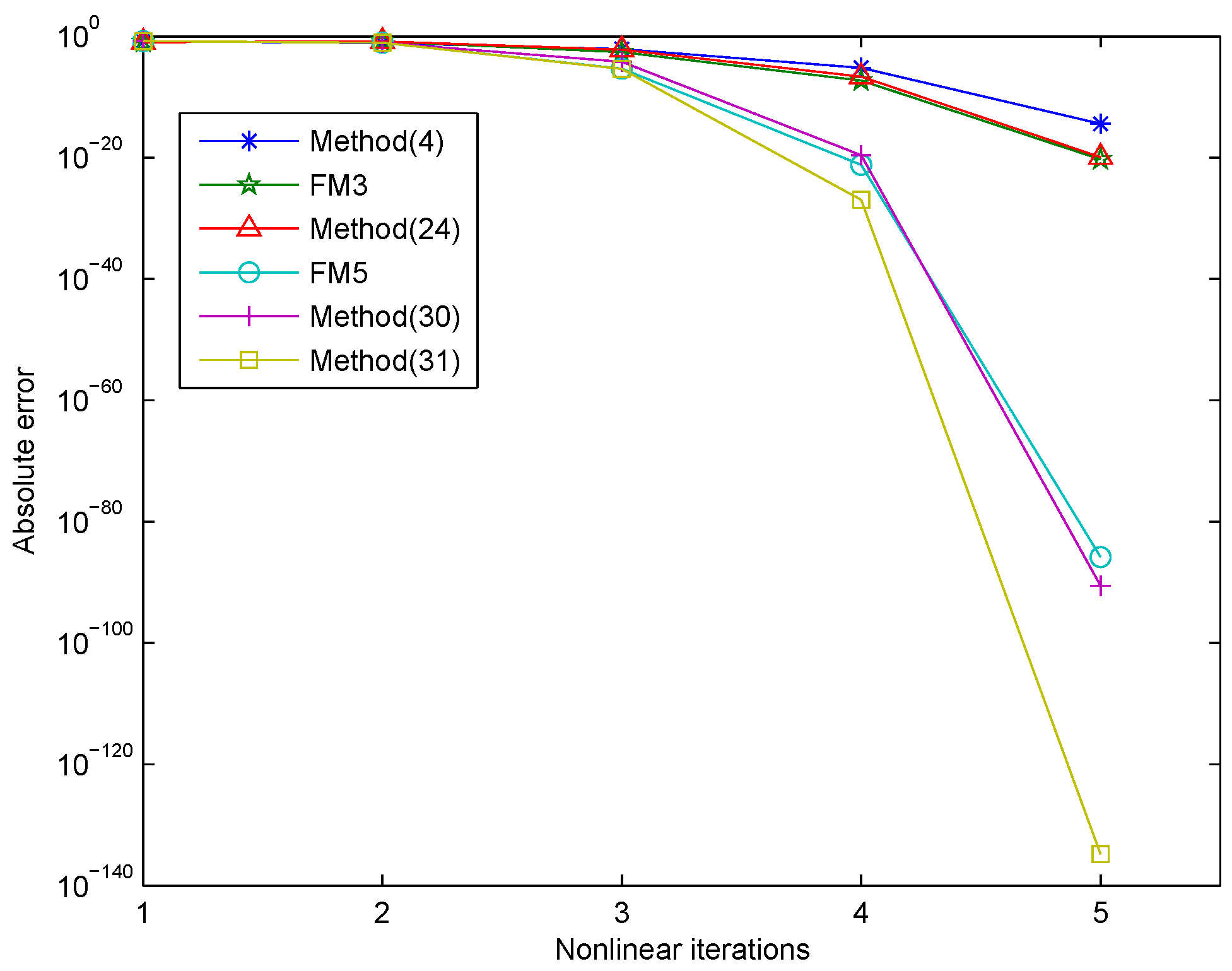
Table 1, Table 2, Table 3, Table 4, Table 5 and Table 6 show the following information: ACOC [12] is the approximated computational order of convergence, NIT (number of iterations) is the number of iterations, EVL is evaluation of error at the last step, T is the CPU time and FU is function values at the last step. The iterative processes of the iterative methods are given by Figure 1, Figure 2, Figure 3, Figure 4 and Figure 5.
Problem 1.
The solution of problem 1 is and the initial value is .
Figure 1 shows that the method in (31) had higher accuracy than the other methods. The accuracy of the method in (24) was similar to that of the FM3 method for Problem 1.
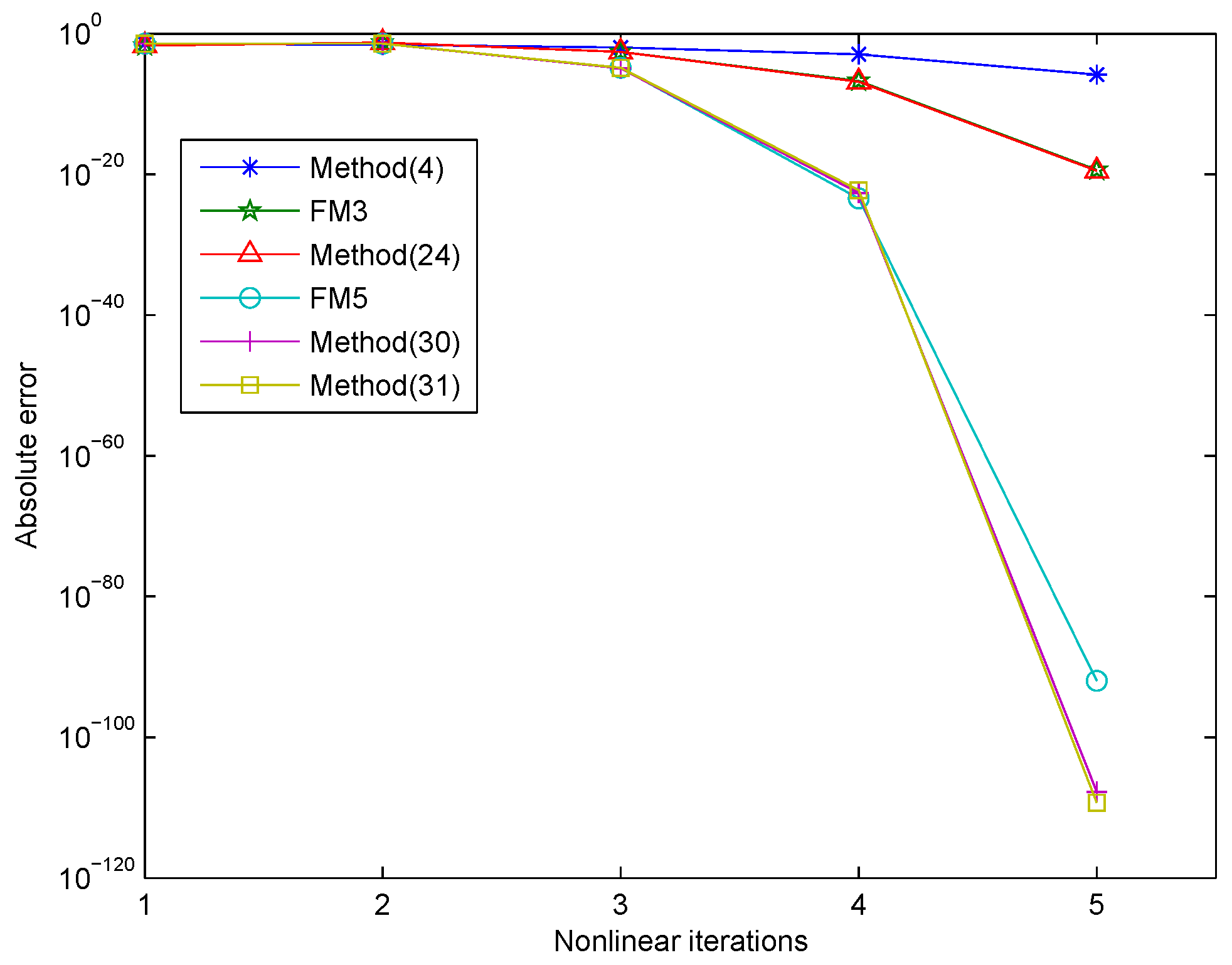
Problem 2.
The solution of Problem 2 is and the initial guess is
Figure 2 shows that the methods in (30) and (31) had higher accuracy than the other methods. The method in (30) and (31) had similar convergence behaviors for Problem 2. The accuracy of the method in (24) was similar to that of the FM3 method for Problem 2.
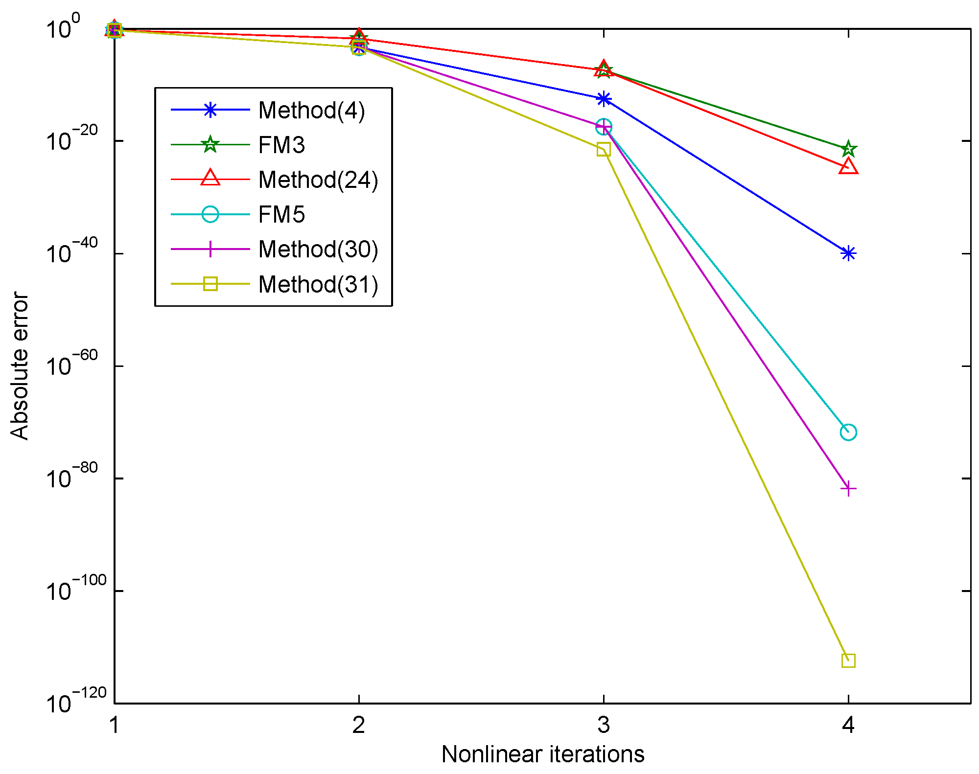
Problem 3.
ODE problem [13]:
Using the discretization method in this problem, we obtain
For we chose the initial value and obtained the solution . The numerical results are shown in Table 3.
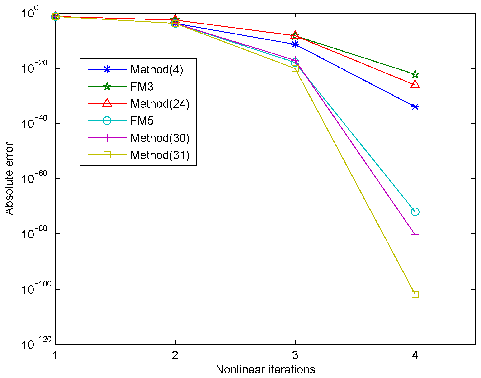
Figure 3 shows that our method, shown in (31), had higher accuracy than the other methods under the same number of iterations.
Problem 4.
ODE problem [14]:
The interval was partitioned into n intervals with a step size of . Using the difference method to discrete the derivative, we obtained
and
We obtained
For , we chose the initial value and obtained the solution . The numerical results are shown in Table 4.
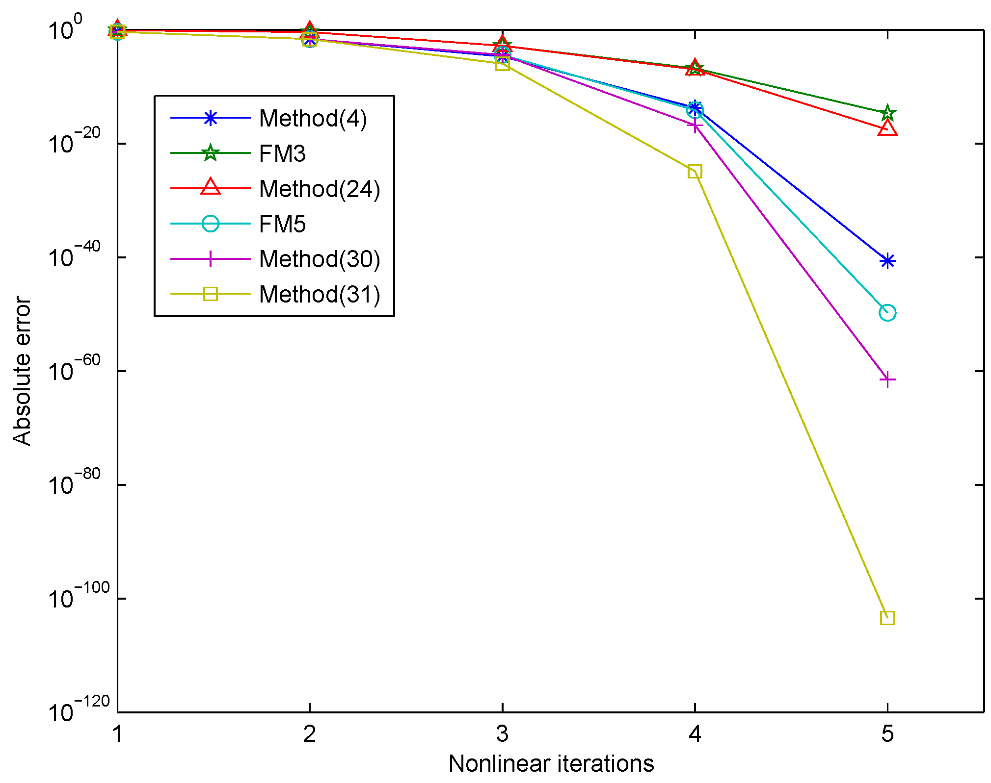
Problem 5.
The solution is and the initial value is .
Problem 6.
Heat conduction problem [15]:
This problem was transformed into nonlinear systems. The step size for t was and the step size for x was . Let , , and ; we obtained
4. Dynamical Analysis
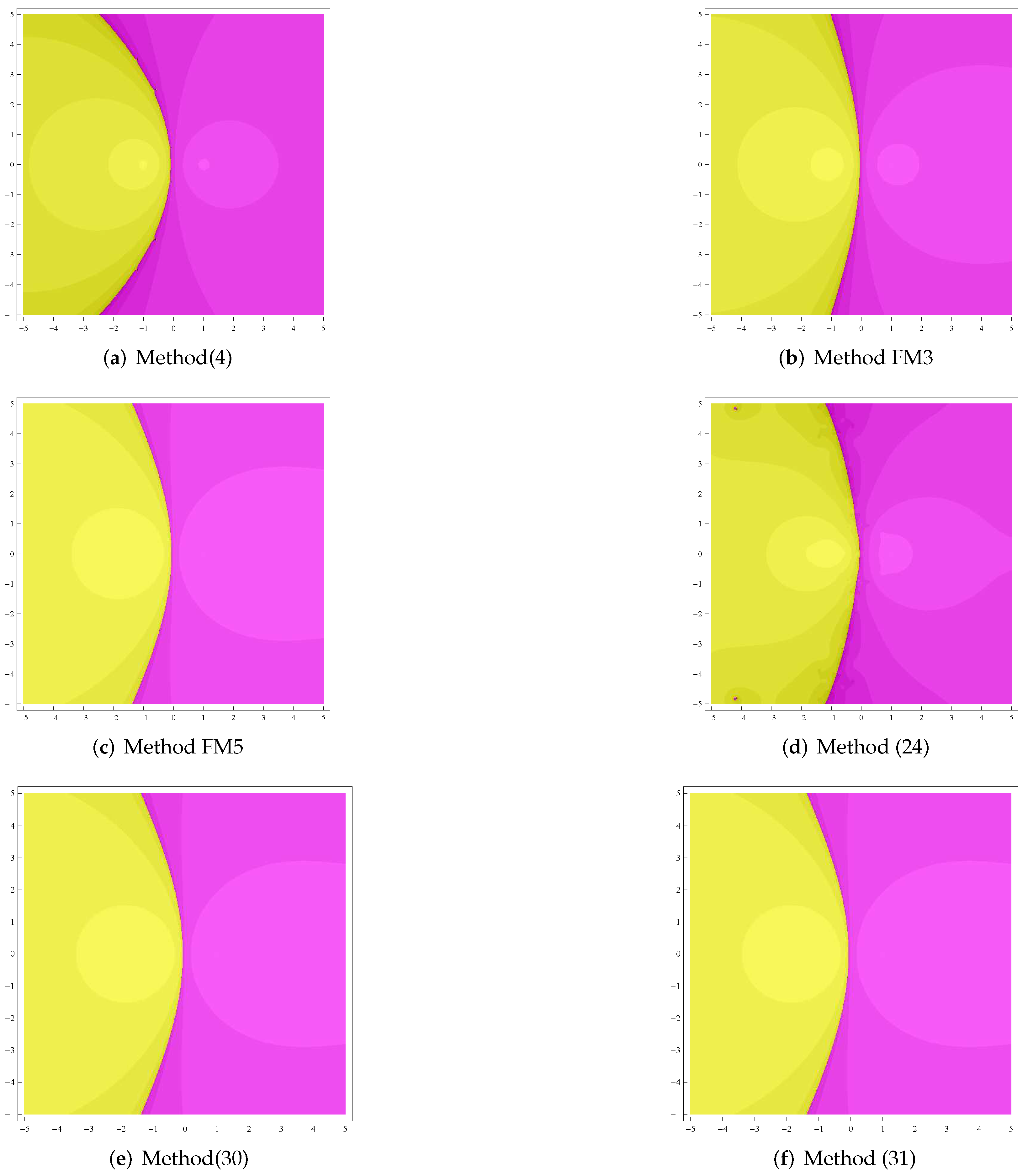
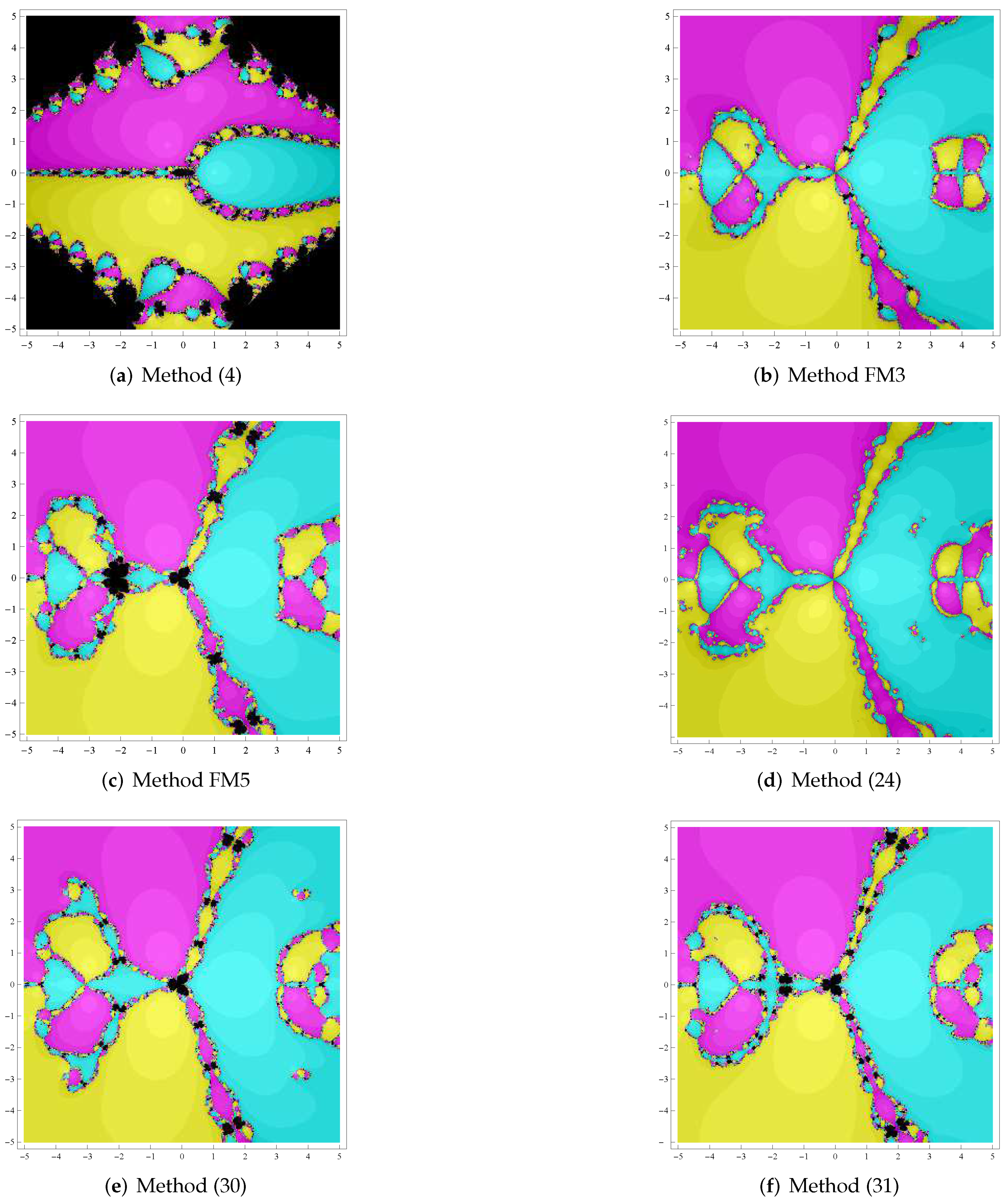
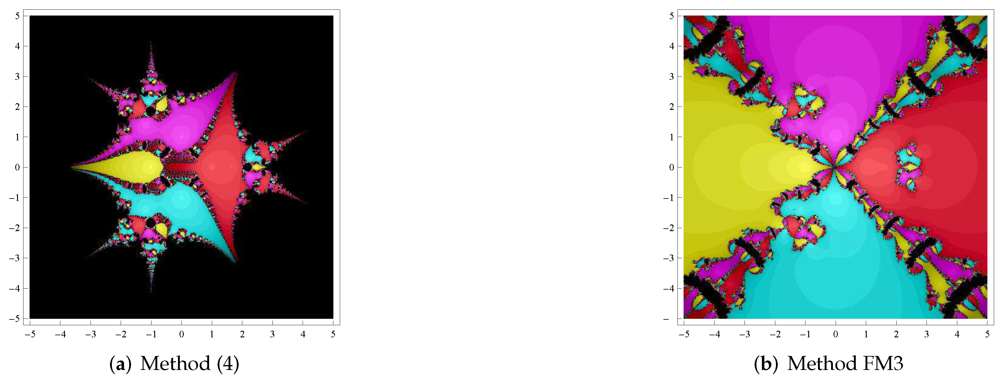
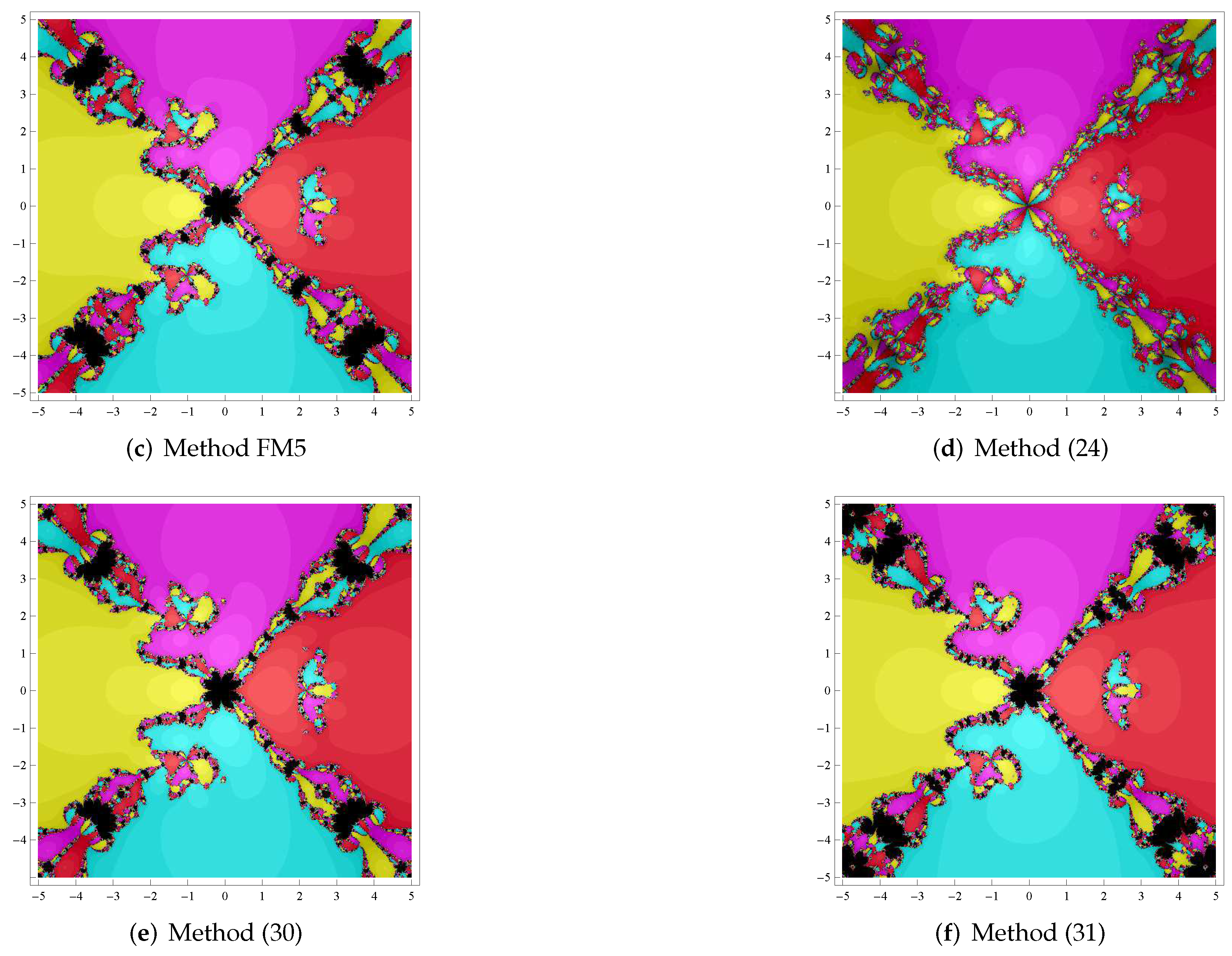
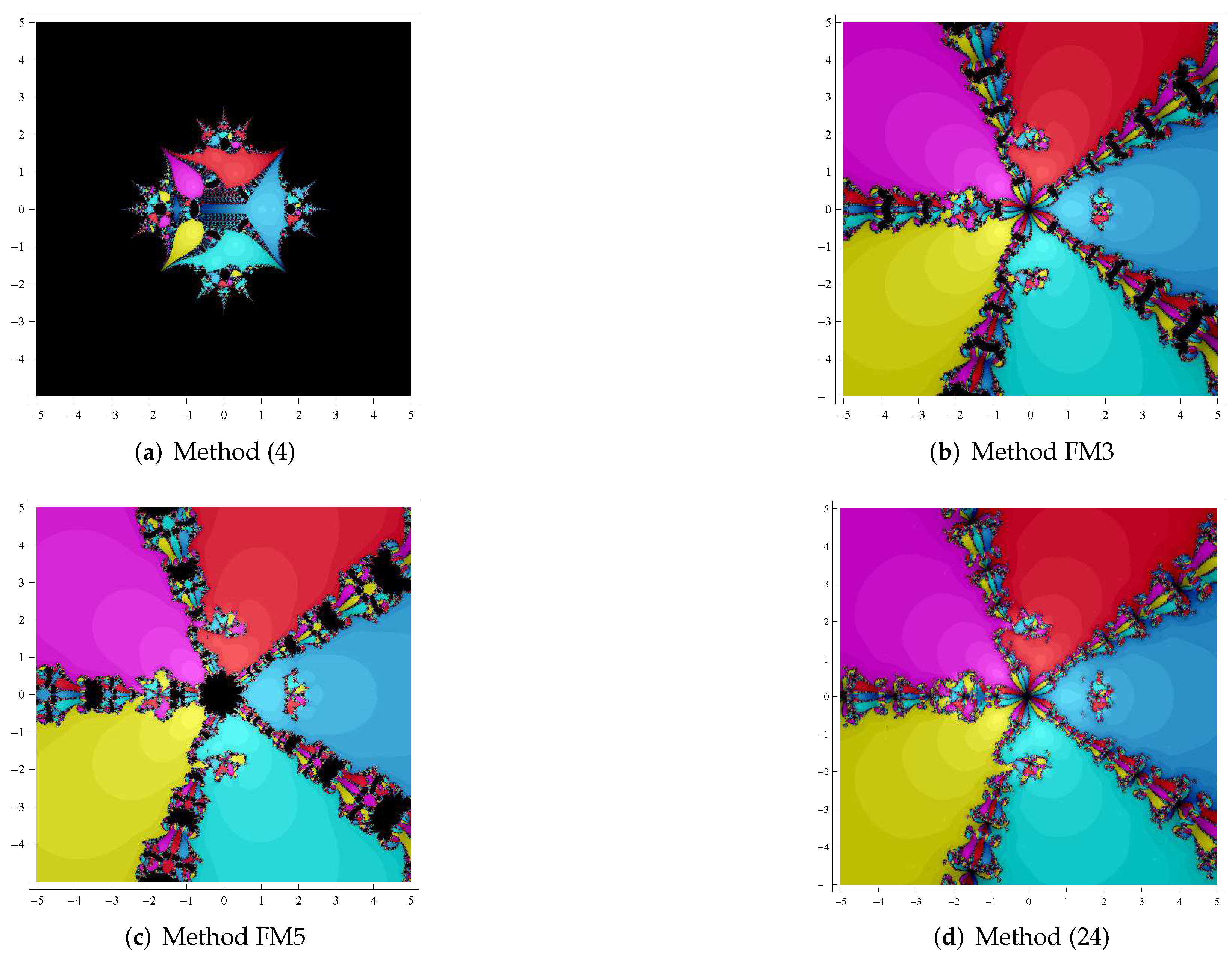
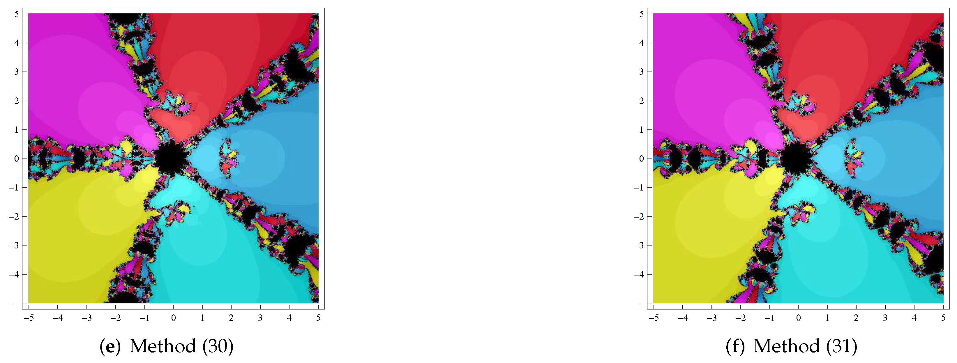
Recently, the dynamical analysis method has been applied to study the stability of the iterative method. Some basic concepts on complex dynamics can be found in references [16,17,18,19,20,21,22,23,24]. For brevity, we omit these concepts in this section. If an iterative method has good stability, it must has good properties for solving simple nonlinear equations. So, we compared our methods with other methods for solving complex equations . The field was divided into a grid of . If the initial point did not converge to the zero of the function after 25 iterations, it was painted with black. The tolerance was used in our programs. Table 7, Table 8, Table 9 and Table 10 show the computing time (Time) for drawing the dynamical planes and the percentage of points (POPs) which guaranteed the convergence to the roots of the complex equations .
5. Conclusions
In this paper, three Kurchatov-type accelerating iterative schemes with memory were obtained by using two novel Kurchatov-type divided difference operator. The new methods avoided the evaluation of the derivative. The orders of convergence of our methods, shown in (24), (30) and (31), are 3, and 5, respectively. We also corrected the order of convergence of Chicharro’s methods, FM3 and FM5. In experimental application, our methods were applied to nonlinear ODEs and PDEs. The numerical results show that, compared with other methods, our methods, shown in (30) and (31), had higher computational accuracy. Dynamical planes were used to analyze the stability of the presented methods. It is worth noting that our method with memory, shown in (24), had better stability than the other methods in this paper. The stability of the method without memory in (4) was the worst. We can conclude that iterative methods with memory can effectively improve the stability of iterative methods without memory.
Author Contributions
Methodology, X.W.; writing—original draft preparation, X.W.; writing—review and editing, X.C. All authors have read and agreed to the published version of the manuscript.
Funding
This research study was supported by the National Natural Science Foundation of China (Nos. 61976027), Educational Commission Foundation of Liaoning Province of China (Nos. LJ2019010), National Natural Science Foundation of Liaoning Province (No. 2019-ZD-0502) and LiaoNing Revitalization Talents Program (XLYC2008002).
Conflicts of Interest
The authors declare no conflict of interest.
References
- Ortega, J.M.; Rheinbolt, W.C. Iterative Solution of Nonlinear Equations in Several Variables; Academic Press: New York, NY, USA, 1970. [Google Scholar]
- Traub, J.F. Iterative Methods for the Solution of Equations; Prentice-Hall: Hoboken, NJ, USA, 1964. [Google Scholar]
- Grau-Sánchez, M.; Noguera, M.; Amat, S. On the approximation of derivatives using divided difference operators preserving the local convergence order of iterative methods. J. Comput. Appl. Math. 2013, 237, 363–372. [Google Scholar] [CrossRef]
- Chicharro, F.I.; Cordero, A.; Garrido, N.; Torregrosa, J.R. On the improvement of the order of convergence of iterative methods for solving nonlinear systems by means of memory. Appl. Math. Lett. 2020, 104, 106277. [Google Scholar] [CrossRef]
- Ahmad, F.; Soleymani, F.; Haghani, F.K.; Serra-Capizzano, S. Higher order derivative-free iterative methods with and without memory for systems of nonlinear equations. Appl. Math. Comput. 2017, 314, 199–211. [Google Scholar] [CrossRef]
- Petković, M.S.; Sharma, J.R. On some efficient derivative-free iterative methods with memory for solving systems of nonlinear equations. Numer. Algorithms 2016, 71, 457–474. [Google Scholar] [CrossRef]
- Kurchatov, V.A. On a method of linear interpolation for the solution of functional equations. Dokl. Akad. Nauk SSSR 1971, 198, 524–526. [Google Scholar]
- Argyros, I.K. On a two-point Newton-like method of convergent order two. Int. J. Comput. Math. 2005, 88, 219–234. [Google Scholar] [CrossRef]
- Argyros, I.K.; Ren, H. On the Kurchatov method for solving equations under weak conditions. Appl. Math. Comput. 2016, 273, 98–113. [Google Scholar] [CrossRef]
- Wang, X.; Jin, Y.; Zhao, Y. Derivative-Free Iterative Methods with Some Kurchatov-Type Accelerating Parameters for Solving Nonlinear Systems. Symmetry 2021, 13, 943. [Google Scholar] [CrossRef]
- Cordero, A.; Soleymani, F.; Torregrosa, J.R.; Khaksar Haghani, F. A family of Kurchatov-type methods and its stability. Appl. Math. Comput. 2017, 294, 264–279. [Google Scholar] [CrossRef] [Green Version]
- Weerakoon, S.; Fernando, T.G.I. A variant of Newton’s method with accelerated third-order convergence. Appl. Math. Lett. 2000, 13, 87–93. [Google Scholar] [CrossRef]
- Ahmad, F.; Rehman, S.U.; Ullah, M.Z.; Aljahdali, H.M.; Ahmad, S.; Alshomrani, A.S.; Carrasco, J.A.; Ahmad, S.; Sivasankaran, S. Frozen Jocabian multistep iterative method for solving nonlinear IVPs and BVPs. Complexity 2017, 2017, 9407656. [Google Scholar] [CrossRef]
- Narang, M.; Bhatia, S.; Kanwar, V. New efficient derivative free family of seventh-order methods for solving systems of nonlinear equations. Numer. Algorithms 2017, 76, 283–307. [Google Scholar] [CrossRef]
- Cordero, A.; Gómez, E.; Torregrosa, J.R. Efficient High-order iterative methods for solving nonlinear systems and their appliation on Heat Conduction Problems. Complexity 2017, 2017, 6457532. [Google Scholar] [CrossRef] [Green Version]
- Lee, M.Y.; Kim, Y.I. The dynamical analysis of a uniparametric family of three-point optimal eighth-order multiple-root finders under the Möbius conjugacy map on the Riemann sphere. Numer. Algorithms 2020, 83, 1063–1090. [Google Scholar] [CrossRef]
- Geum, Y.H.; Kim, Y.I.; Magreñán, Á.A. A biparametric extension of King’s fourth-order methods and their dynamics. Appl. Math. Comput. 2016, 282, 254–275. [Google Scholar] [CrossRef]
- Behl, R.; Cordero, A.; Torregrosa, J.R. High order family of multivariate iterative methods: Convergence and stability. J. Comput. Appl. Math. 2020, 405, 113053. [Google Scholar] [CrossRef]
- Neta, B.; Scott, M.; Chun, C. Basin attrators for various methods for multiple roots. Appl. Math. Comput. 2012, 218, 5043–5066. [Google Scholar]
- Argyros, I.K.; Magreñán, Á.A. Iterative Methods and Their Dynamics with Applications: A Contemporary Study; CRC Press: Boca Raton, FL, USA, 2017. [Google Scholar]
- Kotarski, W.; Gdawiec, K.; Lisowska, A. Polynomiography via Ishikawa and Mann iterations. In Proceedings of the International Symposium on Visual Computing; Springer: Berlin/Heidelberg, Germany, 2021; pp. 305–313. [Google Scholar]
- Susanto, H.; Karjanto, N. Newton’s method’s basins of attraction revisited. Appl. Math. Comput. 2009, 215, 1084–1090. [Google Scholar] [CrossRef] [Green Version]
- Deng, J.J.; Chiang, H.D. Convergence region of Newton iterative power flow method: Numerical studies. J. Appl. Math. 2013, 2013, 509496. [Google Scholar] [CrossRef] [Green Version]
- Ardelean, G. A comparison between iterative methods by using the basins of attraction. Appl. Math. Comput. 2011, 218, 88–95. [Google Scholar] [CrossRef]
Figure 1.
The iterative processes of iterative methods for Problem 1.

Figure 2.
The iterative processes of iterative methods for Problem 2.

Figure 3.
The iterative processes of iterative methods for Problem 3.

Figure 4.
The iterative processes of iterative methods for Problem 4.

Figure 5.
The iterative processes of iterative methods for Problem 5.

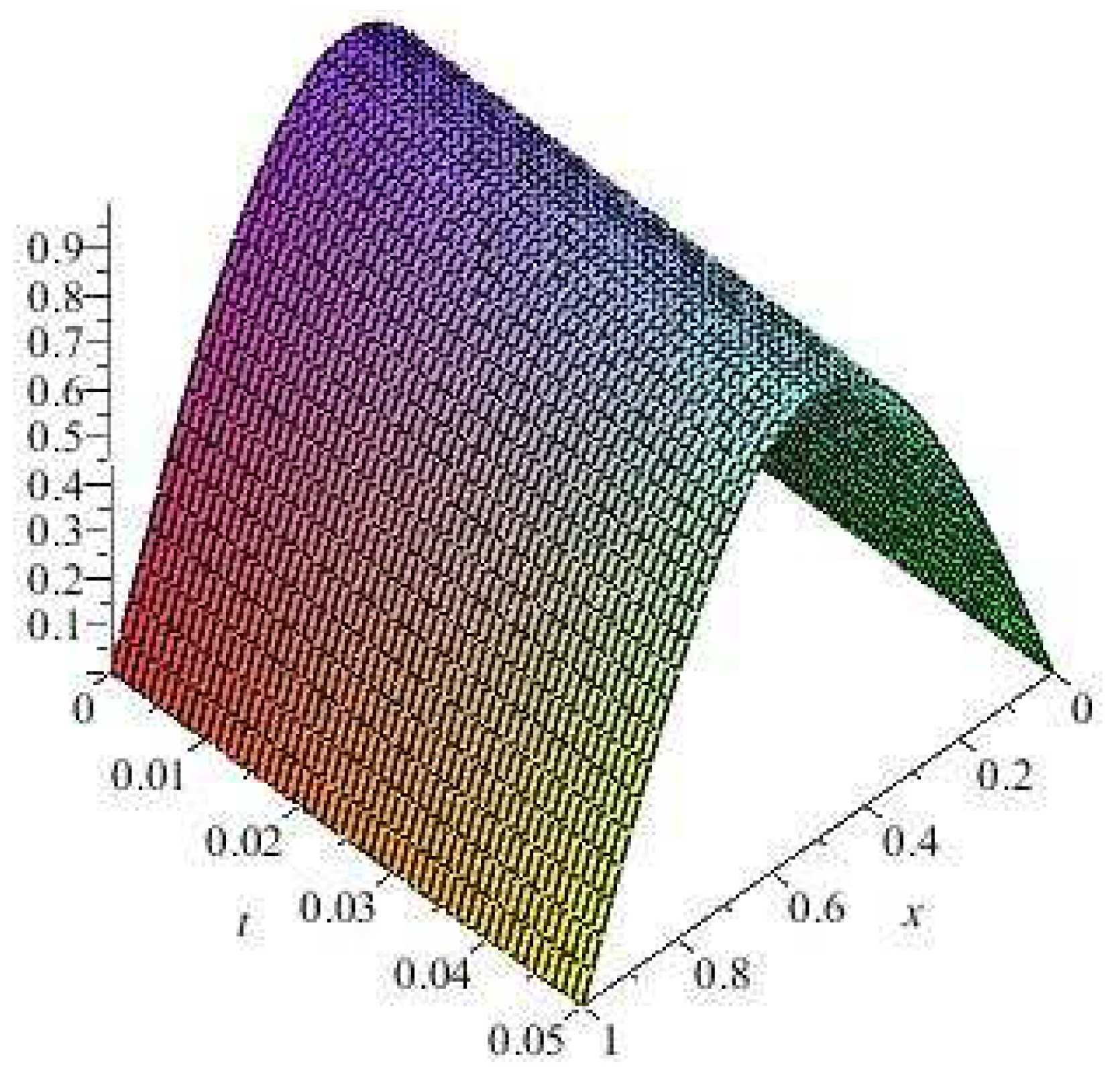
Figure 6.
The exact solutions of Example 6.

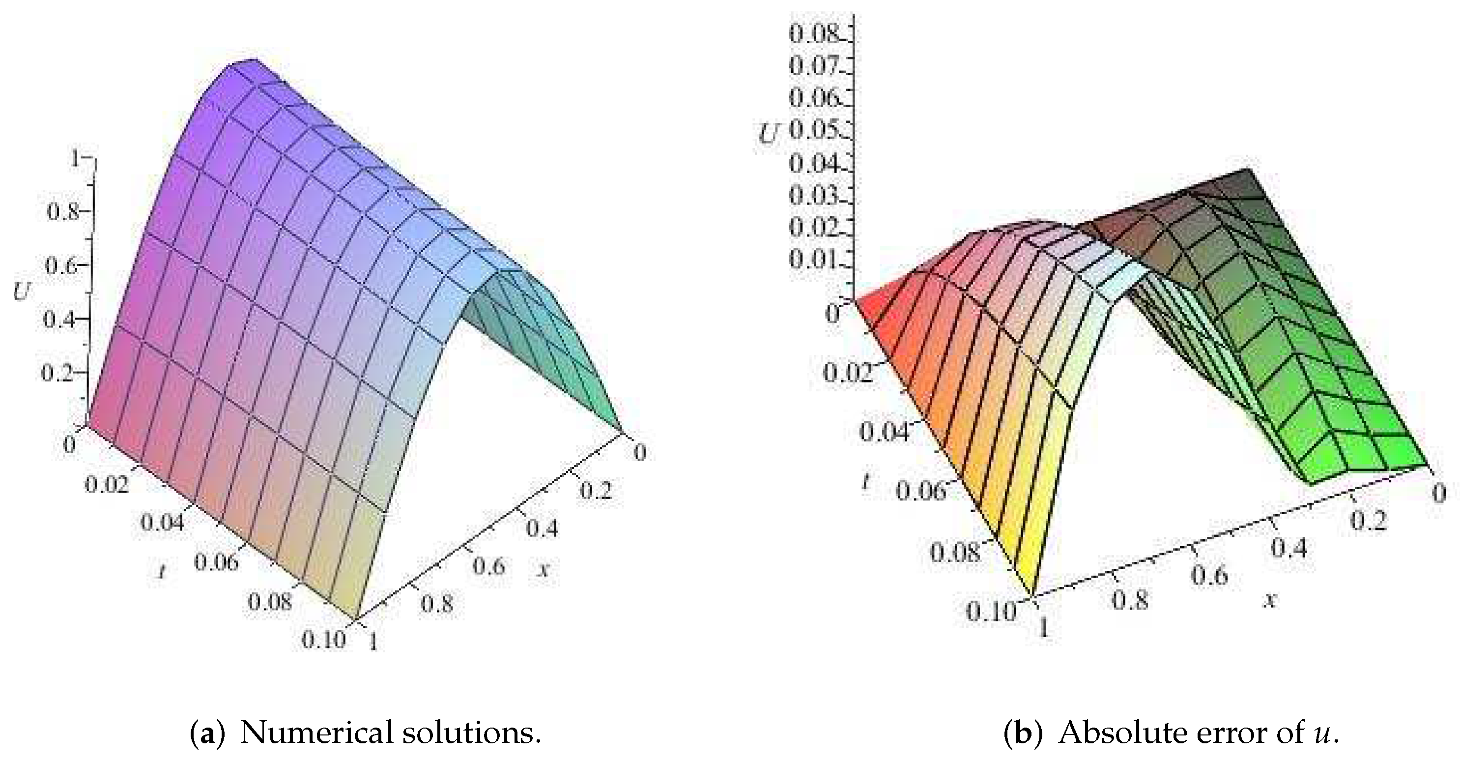
Figure 7.
Numerical solutions (a) of Example 6 (n = 10) produced by the method (b) in (31).

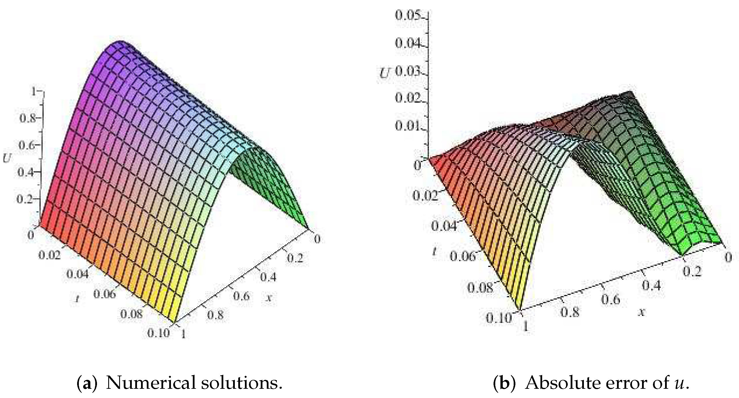
Figure 8.
Numerical solutions (a) of Example 6 (n = 20) produced by the method (b) in (31).

Figure 9.
Dynamical planes for . (a) Method (4), (b) Method FM3, (c) Method FM5, (d) Method (24), (e) Method (30), (f) Method (31).
Figure 9.
Dynamical planes for . (a) Method (4), (b) Method FM3, (c) Method FM5, (d) Method (24), (e) Method (30), (f) Method (31).

Figure 10.
Dynamical planes for . (a) Method (4), (b) Method FM3, (c) Method FM5, (d) Method (24), (e) Method (30), (f) Method (31).
Figure 10.
Dynamical planes for . (a) Method (4), (b) Method FM3, (c) Method FM5, (d) Method (24), (e) Method (30), (f) Method (31).

Figure 11.
Dynamical planes for . (a) Method (4), (b) Method FM3, (c) Method FM5, (d) Method (24), (e) Method (30), (f) Method (31).
Figure 11.
Dynamical planes for . (a) Method (4), (b) Method FM3, (c) Method FM5, (d) Method (24), (e) Method (30), (f) Method (31).


Figure 12.
Dynamical planes for . (a) Method (4), (b) Method FM3, (c) Method FM5, (d) Method (24), (e) Method (30), (f) Method (31).
Figure 12.
Dynamical planes for . (a) Method (4), (b) Method FM3, (c) Method FM5, (d) Method (24), (e) Method (30), (f) Method (31).


Table 1.
Numerical results of different iterative methods for Problem 1.
| Methods | NIT | EVL | FU | ACOC |
|---|---|---|---|---|
| (4) | 7 | 7.931 | 2.395 | 3.00000 |
| FM3 | 7 | 6.263 | 2.601 | 2.73574 |
| (24) | 7 | 5.070 | 3.909 | 3.00000 |
| FM5 | 6 | 6.709 | 4.721 | 3.98043 |
| (30) | 6 | 3.068 | 1.153 | 4.56599 |
| (31) | 5 | 1.667 | 3.865 | 5.00108 |
Table 2.
Numerical results of different iterative methods for Problem 2.
| Methods | NIT | EVL | FU | ACOC |
|---|---|---|---|---|
| (4) | 8 | 1.094 | 1.999 | 3.00000 |
| FM3 | 7 | 2.310 | 8.319 | 2.74317 |
| (24) | 7 | 3.056 | 3.356 | 3.00000 |
| FM5 | 6 | 8.076 | 2.939 | 4.08488 |
| (30) | 5 | 1.821 | 2.669 | 4.79681 |
| (31) | 5 | 5.055 | 3.685 | 4.99999 |
Table 3.
Numerical results of different iterative methods for Problem 3.
| Methods | NIT | EVL | FU | T | ACOC |
|---|---|---|---|---|---|
| (4) | 5 | 5.500 | 5.095 | 567.141 | 3.00009 |
| FM3 | 6 | 2.718 | 1.667 | 405.072 | 2.71295 |
| (24) | 6 | 6.628 | 8.935 | 411.702 | 3.00001 |
| FM5 | 5 | 5.078 | 8.678 | 502.058 | 4.04268 |
| (30) | 5 | 9.412 | 2.431 | 484.133 | 4.55973 |
| (31) | 4 | 4.154 | 1.123 | 377.491 | 5.01082 |
Table 4.
Numerical results of different iterative methods for Problem 4.
| Methods | NIT | EVL | FU | T | ACOC |
|---|---|---|---|---|---|
| (4) | 6 | 4.082 | 3.486 | 57.127 | 3.00008 |
| FM3 | 8 | 1.345 | 7.061 | 58.625 | 2.41965 |
| (24) | 7 | 1.185 | 1.976 | 52.385 | 2.70456 |
| FM5 | 6 | 8.223 | 1.566 | 65.614 | 3.54447 |
| (30) | 6 | 1.601 | 1.857 | 65.099 | 3.74370 |
| (31) | 5 | 3.550 | 9.284 | 52.054 | 4.14892 |
Table 5.
Numerical results of different iterative methods for Problem 5.
| Methods | NIT | EVL | FU | ACOC |
|---|---|---|---|---|
| (4) | 5 | 3.143 | 6.433 | 2.99114 |
| FM3 | 6 | 2.325 | 3.396 | 2.71541 |
| (24) | 6 | 5.172 | 7.518 | 2.98298 |
| FM5 | 5 | 8.133 | 2.547 | 4.05479 |
| (30) | 5 | 2.915 | 2.206 | 4.56718 |
| (31) | 4 | 1.441 | 3.107 | 4.99898 |
Table 6.
Numerical results of different methods for Problem 6 (n = 10).
| Methods | (4) | FM3 | (24) | FM5 | (30) | (31) |
|---|---|---|---|---|---|---|
| 5 | 6 | 6 | 4 | 4 | 4 | |
| 47.654 | 48.297 | 47.533 | 48.048 | 47.861 | 47.851 |
Table 7.
Numerical results of different methods for .
| Methods | (4) | FM3 | FM5 | (24) | (30) | (31) |
|---|---|---|---|---|---|---|
| 99.99 % | 100% | 100% | 100% | 100% | 100% | |
| 38.87 | 40.86 | 39.34 | 42.42 | 38.66 | 38.05 |
Table 8.
Numerical results of different methods for .
| Methods | (4) | FM3 | FM5 | (24) | (30) | (31) |
|---|---|---|---|---|---|---|
| 68.53% | 99.45% | 97.25% | 99.96% | 97.96% | 97.70% | |
| 91.04 | 57.38 | 61.09 | 59.27 | 59.28 | 56.58 |
Table 9.
Numerical results of different methods for .
| Methods | (4) | FM3 | FM5 | (24) | (30) | (31) |
|---|---|---|---|---|---|---|
| 21.72% | 92.93% | 91.89% | 99.31% | 92.65% | 89.45% | |
| 159.96 | 87.82 | 92.12 | 99.70 | 99.87 | 87.80 |
Table 10.
Numerical results of different methods for .
| Methods | (4) | FM3 | FM5 | (24) | (30) | (31) |
|---|---|---|---|---|---|---|
| 10.48% | 92.96% | 89.51% | 97.95% | 89.38% | 90.33% | |
| 179.48 | 92.63 | 97.92 | 92.10 | 96.96 | 92.08 |
Publisher’s Note: MDPI stays neutral with regard to jurisdictional claims in published maps and institutional affiliations. |
© 2022 by the authors. Licensee MDPI, Basel, Switzerland. This article is an open access article distributed under the terms and conditions of the Creative Commons Attribution (CC BY) license (https://creativecommons.org/licenses/by/4.0/).
Share and Cite
MDPI and ACS Style
Wang, X.; Chen, X. Derivative-Free Kurchatov-Type Accelerating Iterative Method for Solving Nonlinear Systems: Dynamics and Applications. Fractal Fract. 2022, 6, 59. https://doi.org/10.3390/fractalfract6020059
AMA Style
Wang X, Chen X. Derivative-Free Kurchatov-Type Accelerating Iterative Method for Solving Nonlinear Systems: Dynamics and Applications. Fractal and Fractional. 2022; 6(2):59. https://doi.org/10.3390/fractalfract6020059
Chicago/Turabian StyleWang, Xiaofeng, and Xiaohe Chen. 2022. "Derivative-Free Kurchatov-Type Accelerating Iterative Method for Solving Nonlinear Systems: Dynamics and Applications" Fractal and Fractional 6, no. 2: 59. https://doi.org/10.3390/fractalfract6020059