
Multivariate Fractal Functions in Some Complete Function Spaces and Fractional Integral of Continuous Fractal Functions


Department of Mathematics, IIT Delhi, New Delhi 110016, India
*
Author to whom correspondence should be addressed.
Fractal Fract. 2021, 5(4), 185; https://doi.org/10.3390/fractalfract5040185
Submission received: 24 July 2021
/
Revised: 18 October 2021
/
Accepted: 20 October 2021
/
Published: 25 October 2021
(This article belongs to the Special Issue Fractal Functions and Applications)
Abstract
:There has been a considerable evolution of the theory of fractal interpolation function (FIF) over the last three decades. Recently, we introduced a multivariate analogue of a special class of FIFs, which is referred to as -fractal functions, from the viewpoint of approximation theory. In the current note, we continue our study on multivariate -fractal functions, but in the context of a few complete function spaces. For a class of fractal functions defined on a hyperrectangle in the Euclidean space , we derive conditions on the defining parameters so that the fractal functions are elements of some standard function spaces such as the Lebesgue spaces , Sobolev spaces , and Hölder spaces , which are Banach spaces. As a simple consequence, for some special choices of the parameters, we provide bounds for the Hausdorff dimension of the graph of the corresponding multivariate -fractal function. We shall also hint at an associated notion of fractal operator that maps each multivariate function in one of these function spaces to its fractal counterpart. The latter part of this note establishes that the Riemann–Liouville fractional integral of a continuous multivariate -fractal function is a fractal function of similar kind.
1. Preamble
This note aims to offer a modest contribution to the field of fractal interpolation. In particular, we consider a special class of fractal interpolation functions referred to as the -fractal function, which has played a considerable role in the theory of univariate fractal approximation. Our work in the current note seeks to show that a few results on the construction of univariate -fractal functions in various function spaces and associated fractal operator (see, for instance, [1]) carry over to higher dimensions.
For a prescribed data set in with increasing abscissae, there are multitude of methods to construct a continuous function that maps each to —generally known as interpolation methods—available in the field of classical numerical analysis and approximation theory. Roughly speaking, the fractal interpolation function (FIF for short), as introduced by Barnsley in the original version [2], is a continuous function that interpolates D such that the graph of g, denoted by , is a self-referential set (fractal set). Here the word fractal or self-referential is used to indicate that is the attractor of an iterated function system [3]. That is, roughly, is a finite union of tranformed copies of itself. For a compendium of the theory of FIF and its applications in interpolation and approximation, the reader is referred to the book and monograph [4,5]; the recent articles [6,7,8] may also be of interest.
In her research works on fractal interpolation, Navascués emphasized a special class of univariate FIFs, named -fractal functions, (see, for instance, [9,10]) which garnered a significant amount of research attention in fractal approximation theory. It is our opinion that the notion of -fractal functions assisted the field of fractal interpolation to find connections and consequences in other branches of mathematics such as approximation theory, harmonic analysis, functional analysis and the theory of bases and frames; see, for instance, [11,12]. In the research works reported in [13,14], authors utilized -fractal functions to demonstrate that FIFs can be applied in various constrained approximation problems.
Several extensions of FIF to higher dimensions, in particular, bivariate FIFs or fractal surfaces, have been studied in the literature; see, for example, [4,15,16,17,18,19]. Despite that the -fractal function facilitated the theory of univariate FIF to merge seamlessly with various fields in mathematics, a similar approach to multivariate FIFs was not attempted except for a few research works on bivariate -fractal functions reported lately in [20,21,22]. The aforementioned works on bivariate -fractal functions find their origin, perhaps implicitly, in the general framework for the construction of fractal surfaces introduced in [23].
While an increasing amount of literature is being published in the field of univariate FIFs and fractal surfaces, the research in multivariate FIFs are still inadequate, especially in the framework of -fractal functions. In the context of multivariate FIFs, the ingenious constructions appeared in [24,25], though worth mentioning, do not seem to be suitable for the implementation of the -fractal function formalism. On the other hand, our acquaintance with the univariate and bivariate -fractal functions revealed that the development of multivariate analogue of -fractal function could be highly beneficial for the expansion of multivariate fractal approximation theory. Stimulated by the construction of fractal surface in [23], recently we put forward a satisfactory extension of the Barnsley’s theory of univariate FIF to the multivariate case [26].
In this note, we continue to explore the notion of multivariate -fractal functions. In the first part, we define multivariate -fractal functions in various function spaces such as the Lebesgue spaces , Sobolev spaces , and Hölder spaces . We also hint at some elementary properties of the fractal operator associated with the notion of multivariate -fractal functions.
Fractal dimension is an important parameter of fractal geometry providing information about the geometric structure of the objects that it deals with. There are different notions of fractal dimension, the two most commonly used being the Hausdorff dimension and box dimension [27]. In particular, the Hausdorff dimension and box dimension of the graphs of fractal interpolation functions have been investigated; see, for instance, [2,4,15,28]. Since the aforementioned fractal dimensions are scale-independent, they may not be useful for describing scale-dependent laws and more complicated phenomena in nature. To this end, a new definition of fractal dimension, referred to as the two-scale dimension, is broached in [29], and it is perhaps more akin to physics than mathematics. However, we are forced to settle for less in the framework of multivariate -fractal functions considered herein, because the analysis for the fractal dimension of the general nonaffine case is subtle. We shall just mention bounds for the Hausdorff dimension of the graph of the multivariate -fractal function as an immediate consequence of its Hölder continuity for suitable choice of parameters.
On the other hand, fractional calculus, which broadly deals with derivatives and integrals of fractional order, is rather an old subject. During the last decades, fractional calculus has opened its wings wider to cover several real world applications in science and engineering. Despite being an old subject, fractional calculus continues to be a hot topic of research, resulting in a substantial body of literature; we refer the reader to the informative surveys [30,31]. Some recent developments made in the direction of fractional PDEs and their applications deserve a special mention; see, for instance, [32,33,34,35]. Studies on the interconnection between fractional calculus and fractal geometry have gained significant attention in recent years. For some links between the two-scale problem mentioned previously and fractional calculus, the reader may consult [36]. In the second part of this note, our modest aim is to show that the fractional integral of the multivariate fractal function considered herein is again a fractal function of a similar kind.
Overall, this note discusses how some results in univariate fractal interpolation, to be specific -fractal functions, fractal operator and fractional calculus of fractal functions, carry over to higher dimensions. We strongly believe that these research findings may assist efforts to find interesting interconnections between multivariate FIFs and the theory of PDEs.
2. Preparatory Facts
To begin with, we list pertinent definitions and notation for use throughout the remainder of this note.
The set of first n natural numbers shall be denoted by . For called a multi-index, let Given two multi-indices and we say that if for all For , we define:
Let and be an n-dimensional hyperrectangle, where each is a closed and bounded interval in For a function and , denoted by
provided the right-hand side exists.
2.1. Function Spaces
The purpose here is to provide a short presentation of various function spaces that are used in this note. We refer to Triebel [37] for more information.
Let denote the Banach space of all real-valued continuous functions defined on , endowed with the sup-norm . For a positive integer m, we consider the linear space defined by
For any , we define
It is well-known that equipped with is a Banach space. Next, we recall the Lebesgue spaces. For let
where is defined as
It is a standard result in functional analysis that is a Banach space for . For is a quasi-norm, that is, in place of the triangle inequality one has
and is a quasi-Banach space.
Let For a multi-index a function is called the -weak derivative of g if it satisfies
for all infinitely differentiable functions with compact support contained in By a slight abuse of notation, we write -weak derivative of g as
For and a non-negative integer denotes the Sobolev space with smoothness m and integrability p defined by
The linear space endowed with the norm
is a Banach space. For , it is a Hilbert space, which shall be denoted by
A function is Hölder continuous with exponent (or - Hölder continuous) if
for all and some , called a Hölder constant of g. Given a Hölder continuous with exponent the -Hölder semi-norm of g is defined by
If m is a positive integer, then the Hölder space is defined as
The space equipped with the norm
is a Banach space. Note that coincides with the space of all Hölder continuous functions with exponent .
2.2. Towards Multivariate FIF
Here we shall equip ourselves with a few rudiments needed for multivariate fractal functions that concern us. As mentioned previously, let , be compact intervals in and be an n-dimensional hyperrectangle.
Let be an integer and ; be such that for each . Note that determines a partition of into subintervals for and . It is worth to note that and each knot point in the partition of is exactly in one of the subintervals , mentioned above. We call such a set as a partition of for an obvious reason.
For convenience, let us introduce the following notation. For a positive integer
For each let be an affine map of the form
satisfying
When the interval involved in the definition of the affine map is half-open, the above equation needs to be interpreted in terms of the one-sided limit. For instance, when is odd, in (1) actually means .
Note that
for . Using the definition of the map , one can verify that
for all
Let be defined by
Using the above notation, we see that for all and
It is easy to observe that the boundary of in the usual metric of is
3. Multivariate -Fractal Functions in Some Complete Function Spaces
This section targets to construct fractal functions (self-referential functions) in the complete function spaces , , and , which we recalled in the previous section. To this end, let be any of the function space from the list , and be a fixed function, which we shall refer to as the germ function. Let be a fixed function, called the base function.
For each , and we define as
where and are real numbers such that
The -tuple comprised of the real numbers is called the scaling vector and it is denoted by . We define
The main objective in this section is to choose the scale vector and base function b in (5) so that the Read-Bajraktarević (RB) operator is a well-defined map, and, in fact, is a contraction map on the function or a suitable subspace of . It is worth to emphasize that throughout the current note, a partition of the hyperrectangle is chosen as mentioned in the previous section.
Theorem 1.
Let and define
Suppose that the scaling vector α is so chosen that
and .
Then the following hold.
- The map given in (5) is well-defined on .
- In fact, is a contraction map.
- As a consequence, by the Banach fixed point theorem, there exists a unique function such thatfor all and multi-index l with Moreover, the function and its derivatives satisfy the self-referential equations given byfor all , and multi-index l with
Proof.
We shall first show that is well-defined on , that is, we show that for all
Let and be such that for some and
Note that this is possible only when and in that case, by (3), we have
and So, by the specified choice of b, we have
for all multi-index l with Thus,
That is, irrespective of whether is considered as a point in or as a point in The above observation also yields the following:
- for all and
- for all and
In particular, .
Next, let and l be a multi-index with Then
Taking sum over all , we get
Since, the map is a contraction. Rest of the claim follows by a simple application of the Banach fixed point theorem. □
Example 1.
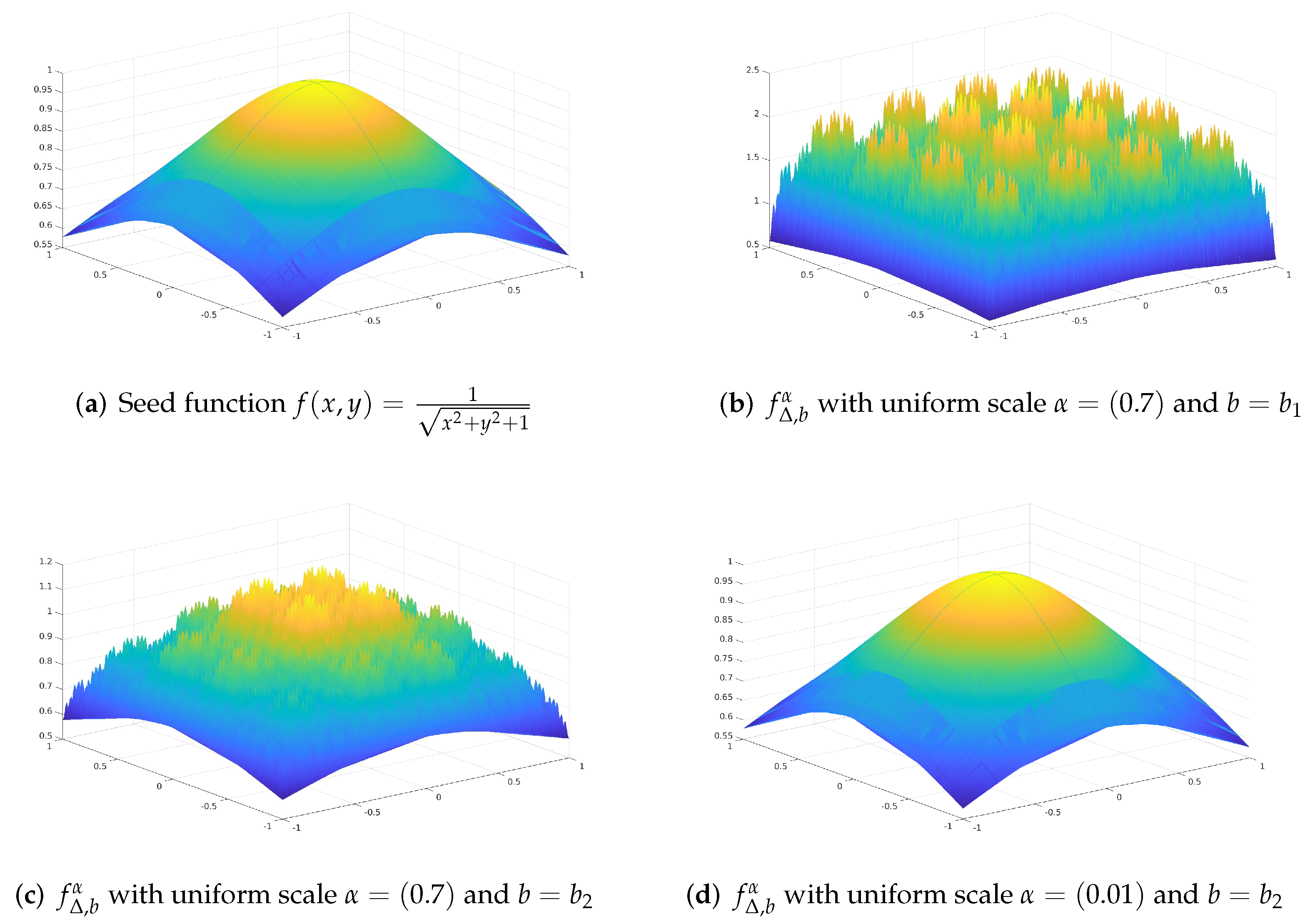
Let us consider the surface indefined by the bivariate functionfor alland a mesh partitionof the squareFractal functionscorresponding tofassociated with different choices of scale vectorand base function b are shown below.
Let us consider two base functions as follows:
and
Figure 1a is the graph of the germ function Figure 1b is the graph of fractal perturbation with base function and uniform scale vector , where for all for . Figure 1c depicts the graph of with base function and uniform scale vector as taken previously. Finally, Figure 1d displays the graph of with base function and uniform scale vector , where . In this case, the parameters satisfy the conditions prescribed in Theorem 1, for . Thus, Figure 1a,b corroborate the technique demonstrated for the construction of smoothness preserving fractal functions in Theorem 1.
Theorem 2.
Let and define
Choose the scale vector satisfying
Proof.
Using Theorem 1 we see that for all . We shall show that for all multi-index l with , is Hölder continuous with exponent . Towards this, let be two points in the same rectangular mesh. We have
where and denote the Hölder constants of and , respectively. If X and Y lie in two distinct but in adjacent meshes, then by taking point on their common boundary and repeating the above steps we get
Since the total number of rectangular meshes is for any , we have
which shows that .
A similar computation reveals also that the map is a contraction map, completing the proof. □
Corollary 1.
Letbe a Hölder continuous function with exponent. Assume that a scaling vectoris so chosen that
and the parameter mapbis a Hölder continuous function with exponentandfor all. Then the Hausdorff dimension of the graph of the corresponding self-referential functionsatisfies
Proof.
With the stated hypotheses on and b, it follows from the previous theorem (with ) that the self-referential counterpart of f is a Hölder continuous function with exponent . Define a map by
where we endow and with the usual Euclidean norm. It is plain to see that A is a surjective Lipschitz map. From fundamental properties of the Hausdorff dimension given in ([38], Theorem 2, Items (5), (8)) we have
For the desired upper bound, let us recall that the Hausdorff dimension of the graph of a Hölder continuous function with Hölder exponent whose domain is a compact subset of with the Hausdorff dimension equal to d is less than or equal to ([39], Chapter 10). Therefore,
completing the proof. □
Theorem 3.
Let for Suppose the scaling vector α is so chosen that
Then defined in (5) maps to . Further, is a contraction map and hence by the Banach fixed point theorem, there exists a unique such that
for and
Proof.
Using the stated hypotheses, it is easy to verify that the operator is well-defined. What remains is to show that is a contraction map. To this end, let We have
Thus,
proving the claim for the case . The other cases can be dealt similarly. □
Next, let us construct self-referential functions associated with a function First, let us recall the following result, popularly known as the Leibniz theorem.
If and is infinitely differentiable on , then and
Theorem 4.
Let for . Suppose that the base function and the scaling vector is chosen so that
Then the RB operator given in (5) is a contraction map on Consequently, has a unique fixed point .
Proof.
A routine computation yields that the RB operator is well-defined and it maps the space into itself. We shall just show that it is a contraction on To this end, let and l be a multi-index with We note that
Thus, for a multi-index l with we have
Hence,
The rest of the theorem follows from the Banach fixed point theorem and the assumption on the scale vector. The case can be worked out similarly. □
4. Fractal Operator on Function Spaces
Let , where is a fixed function space from the list
The results established in the previous section provide a self-referential counterpart to each , and consequently provide an operator. That is, for a prescribed set of parameters such as the partition, scale vector and the base function, there exists a fractal operator defined by This section intends to record a few elementary properties of the operator , what we call a multivariate self-referential operator (fractal operator); see also [1]. We shall provide the details only for , as the other spaces can be similarly dealt with. For future reference, we introduce the notation
Proposition 1.
(Perturbation Error) Let. Suppose that a partitionof the hyperrectangle, base function, and scale vectorbe chosen as in Theorem 4. Then
Proof.
Let us recall the self-referential equations satisfied by the fractal counterpart and its derivatives
for all , and multi-index l with Assume that . By simple calculations
Therefore,
Similar analysis for . □
Now, let us take the multivariate base function used in the construction of the self-referential function through a suitable operator . That is, we take so that the conditions required for b are satisfied. In this case, the multivariate fractal operator will be denoted by In what follows, we intend to record some elementary properties of the multivariate fractal operator .
The following proposition provides a counterpart to the linearity property of the fractal operator well explored in the setting of univariate -fractal functions on various function spaces; see, for instance, [11]. The proof follows almost verbatim, and hence omitted.
Proposition 2.
Letandbe a linear operator. Choose the base functionbin the construction of fractal functionvia this operatorLso that. Then the corresponding fractal operator, which shall be denoted by, defined byis linear.
Let X be a Banach space and be a bounded linear operator such that , where I is the identity operator on X. Then, it is well-known that A is bijective and is bounded; see, for instance, [40]. The following result available in [41] is a generalization of the aforementioned Neumann’s lemma.
Lemma 1.
for some and Then A is a topological automorphism (a bounded, invertible map that possesses a bounded inverse). Furthermore,
Proposition 3.
Letbe a bounded linear operator and the scale vectorbe chosen such that. Then the linear operatoris a topological automorphism.
Proof.
Recall that here the base function so that by Proposition 1 we have
The assertion is now immediate from the previous proposition. □
The existence of Schauder bases consisting of appropriate functions for the Sobolev spaces is quite desirable in analysis of PDEs, for instance, for demonstrating the existence of solutions of various non-linear boundary value problems. We have the following result giving a Schauder basis consisting of self-referential functions for the Sobolev space . The heart of the matter is an elementary result in the theory of bases, which states that a topological isomorphism preserves Schauder bases; see, for instance, [37].
Corollary 2.
The Banach spacehas a Schauder basis consisting of multivariate self-referential functions.
Proof.
Let be a Schauder basis of whose existence is established and reported, for instance, in [42,43,44]. Choose the scale function and operator L as in the previous proposition so that the fractal operator is a topological automorphism. As an isomorphism, in particular, an automorphism, preserves Schauder bases, we conclude that , where is a Schauder basis consisting of self-referential functions for the Banach space . □
5. Fractional Integral of Continuous Multivariate -Fractal Function
As mentioned in the introductory section, exploration of interconnection between fractional calculus and fractal geometry has always been of interest. Our purpose in this section is limited; we shall observe that the Riemann–Liouville fractional integral of the continuous multivariate -fractal function is also a fractal function. A similar result regarding univariate FIF can be found in [28].
Definition 1.
[45] Let f be a continuous function on the closed and bounded hyperrectanglein. The left-hand-sided mixed Riemann–Liouville fractional integral of f of orderis defined as
whereis a fixed point,andwith,for each
Let . We write . From Theorem 1 it follows that by choosing and scaling vector such that
the fractal counterpart of f belongs to . Furthermore, since is the fixed point of the RB operator defined by
for all , . Consequently, satisfies the functional equation
Let us define
so that the self-referential equation for becomes
Since the multivariate fractal function is continuous, we can talk about its Riemann–Liouville fractional integral. In what follows, we establish that the Riemann–Liouville fractional integral of is again a fractal function.
For the sake of convenience, we shall deal with the uniform scaling factor, that is, for all Then, with a slight abuse of notation, the above equation reduces to
Theorem 5.
Let Δ be a partition of the hyperrectangle Ω in and . Assume that is continuous and for all , the boundary of Ω. Choose a scaling vector α such that Then , the left-hand-sided mixed Riemann–Liouville fractional integral of order γ of the self-referential function , satisfies the following equation:
where
Proof.
According to Theorem 1, it follows that is continuous on and satisfies the equation
Hence,
Let us write
so that
Turning our attention to , let us change the variable using the transformation . We have
Applying similar process to the variable we get
In , let us perform a change of variable using so that
Consequently,
Proceeding in the same fashion, at the step we get
where
for , with the assumption that
Finally, using the functional equation
for all , we get
as desired. □
6. Conclusions
The -fractal formalism of fractal interpolation function is proved to be beneficial in expanding the applications of univariate fractal approximation theory. Through the construction of multivariate -fractal functions on a few complete function spaces which are ubiquitous in the theory of partial differential equations and harmonic analysis, the present work intends to be a step forward in the theory of multivariate fractal approximation. The construction of self-referential analogue for each germ function in a complete function space under consideration leads naturally to an operator, referred to as the multivariate fractal operator. We have studied a few elementary properties of the fractal operator. The multivariate fractal operator introduced and studied here enabled us, in particular, to construct Schauder bases consisting of self-referential functions for the function spaces. Further, taking a slight detour from the main theme, it is shown that the Riemann–Liouville fractional integral of a self-referential counterpart of the given multivariate germ function will also be a self-referential function under some suitable conditions.
Author Contributions
Conceptualization, P.V.V.; Methodology, K.K.P. and P.V.V.; Supervision, P.V.V.; Writing—original draft, K.K.P.; Writing—review & editing, P.V.V. All authors have read and agreed to the published version of the manuscript.
Funding
The second author is thankful to the project CRG/2020/002309 from the Science and Engineering Research Board (SERB), Government of India.
Institutional Review Board Statement
Not applicable.
Informed Consent Statement
Not applicable.
Data Availability Statement
Not applicable.
Acknowledgments
Conflicts of Interest
The authors declare no conflict of interest. The funders had no role in the design of the study; in the collection, analyses, or interpretation of data; in the writing of the manuscript, or in the decision to publish the results
References
- Viswanathan, P.; Navascués, M.A. A Fractal Operator on Some Standard Spaces of Functions. Proc. Edinb. Math. Soc. 2017, 60, 771–786. [Google Scholar] [CrossRef] [Green Version]
- Barnsley, M.F. Fractal functions and interpolation. Constr. Approx. 1986, 2, 303–329. [Google Scholar] [CrossRef]
- Hutchinson, J. Fractals and self-similarity. Indiana Univ. Math. J. 1981, 30, 713–747. [Google Scholar] [CrossRef]
- Massopust, P.R. Fractal Functions, Fractal Surfaces and Wavelets; Academic Press: Cambridge, MA, USA, 2014. [Google Scholar]
- Massopust, P.R. Interpolation and Approximation with Splines and Fractals; Oxford University Press: New York, NY, USA, 2010. [Google Scholar]
- Kok, C.W.; Tam, W.S. Fractal Image Interpolation: A Tutorial and New Result. Fractal Fract. 2019, 3, 7. [Google Scholar] [CrossRef] [Green Version]
- Navascués, M.A.; Chand, A.K.B.; Veedu, V.P.; Sebastián, M.V. Fractal Interpolation Functions: A Short Survey. Appl. Math. 2014, 5, 1834–1841. [Google Scholar] [CrossRef] [Green Version]
- Ri, S., II; Drakopoulos, V.; Nam, S.-M. Fractal Interpolation Using Harmonic Functions on the Koch Curve. Fractal Fract. 2021, 5, 28. [Google Scholar] [CrossRef]
- Navascués, M.A. Fractal polynomial interpolation. Z. Anal. Anwend. 2005, 25, 401–418. [Google Scholar] [CrossRef]
- Navascués, M.A. Fractal trigonometric approximation. Electron. Trans. Numer. Anal. 2005, 20, 64–74. [Google Scholar]
- Navascués, M.A. Fractal approximation. Complex Anal. Oper. Theory 2010, 4, 953–974. [Google Scholar] [CrossRef]
- Navascués, M.A. Fractal bases for Lp-spaces. Fractals 2012, 20, 141–148. [Google Scholar] [CrossRef]
- Viswanathan, P.; Chand, A.K.B.; Navascués, M. Fractal perturbation preserving fundamental shapes: Bounds on the scale factors. J. Math. Anal. Appl. 2014, 419, 804–817. [Google Scholar] [CrossRef]
- Viswanathan, P.; Navascués, M.A.; Chand, A.K.B. Fractal Polynomials and Maps in Approximation of Continuous Functions. Numer. Funct. Anal. Optim. 2015, 37, 106–127. [Google Scholar] [CrossRef]
- Bouboulis, P.; Dalla, L.; Drakopoulos, V. Construction of recurrent bivariate fractal interpolation surfaces and computation of their box-counting dimension. J. Approx. Theory 2006, 141, 99–117. [Google Scholar] [CrossRef] [Green Version]
- Chand, A.K.B.; Kapoor, G.P. Hidden Variable Bivariate Fractal Interpolation Surfaces. Fractals 2003, 11, 277–288. [Google Scholar] [CrossRef]
- Dalla, L. Bivariate fractal interpolation functions on grids. Fractals 2002, 10, 53–58. [Google Scholar] [CrossRef]
- Feng, Z. Variation and Minkowski dimension of fractal interpolation surfaces. J. Math. Anal. Appl. 1993, 176, 561–586. [Google Scholar] [CrossRef] [Green Version]
- Massopust, P.R. Fractal surfaces. J. Math. Anal. Appl. 1990, 151, 275–290. [Google Scholar] [CrossRef] [Green Version]
- Navascues, M.A.; Mohapatra, R.N.; Akhtar, M.N. Construction of Fractal Surfaces. Fractals 2020, 28, 13. [Google Scholar] [CrossRef]
- Verma, S.; Viswanathan, P. A Fractal Operator Associated with Bivariate Fractal Interpolation Functions on Rectangular Grids. Results Math. 2020, 75, 28. [Google Scholar] [CrossRef]
- Verma, S.; Viswanathan, P. Parameter Identification for a Class of Bivariate Fractal Interpolation Functions and Constrained Approximation. Numer. Funct. Anal. Optim. 2020, 41, 1109–1148. [Google Scholar] [CrossRef]
- Ruan, H.-J.; Xu, Q. Fractal interpolation surfaces on rectangular grids. Bull. Aust. Math. Soc. 2015, 91, 435–446. [Google Scholar] [CrossRef]
- Bouboulis, P.; Dalla, L. A general construction of fractal interpolation functions on grids of n. Eur. J. Appl. Math. 2007, 18, 449–476. [Google Scholar] [CrossRef] [Green Version]
- Hardin, D.; Massopust, P.R. Fractal interpolation function from n to m and their projections. Z. Anal. Anw. 1993, 12, 561–586. [Google Scholar]
- Pandey, K.K.; Viswanathan, P. Multivariate fractal interpolation functions: Some approximation aspects and an associated fractal interpolation operator. arXiv 2021, arXiv:2104.02950V1. [Google Scholar]
- Falconer, K. Fractal Geometry—Mathematical Foundations and Applications, 3rd ed.; John Wiley: Hoboken, NJ, USA, 2014. [Google Scholar]
- Ruan, H.-J.; Su, W.-Y.; Yao, K. Box dimension and fractional integral of linear fractal interpolation functions. J. Approx. Theory 2009, 161, 187–197. [Google Scholar] [CrossRef] [Green Version]
- Ain, Q.T.; He, J.-H. On two-scale dimension and its applications. Therm. Sci. 2019, 23, 1707–1712. [Google Scholar] [CrossRef] [Green Version]
- Machado, J.A.T.; Kiryakova, V.; Mainardi, F. Recent history of fractional calculus. Commun. Nonlinear Sci. Numer. Simul. 2011, 16, 1140–1153. [Google Scholar] [CrossRef] [Green Version]
- Sun, H.G.; Zhang, Y.; Baleanu, D.; Chen, W.; Chen, Y. A new collection of rel world applications of fractional calculus in science and engineering. Commun. Nonlinear Sci. Numer. Simul. 2018, 64, 213–231. [Google Scholar] [CrossRef]
- Dai, D.-D.; Ban, T.-T.; Wang, Y.-L.; Zhang, W. The piecewise reproducing kernel method for the time variable fractional order advection-reaction-diffusion equations. Therm. Sci. 2021, 25, 1261–1268. [Google Scholar] [CrossRef]
- Orovio, A.B.; Kay, D.; Burrage, K. Fourier spectral methods for fractional-in-space reaction-diffusion equations. BIT Numer. Math. 2014, 54, 937–954. [Google Scholar] [CrossRef]
- Tian, Y.; Liu, J. A modified exp-function method for fractional partial differential equations. Therm. Sci. 2021, 25, 1237–1241. [Google Scholar] [CrossRef]
- Tian, Y.; Liu, J. Direct algebraic method for solving fractional Fokas equation. Therm. Sci. 2021, 25, 2235–2244. [Google Scholar] [CrossRef]
- He, J.-H.; Ji, F.-Y. Two-scale mathematics and fractional calculus for thermodynamics. Therm. Sci. 2019, 23, 2131–2133. [Google Scholar] [CrossRef]
- Triebel, H. Theory of Function Spaces; Birkhaüser: Basel, Switzerland, 1992. [Google Scholar]
- Schleicher, D. Hausdorff dimension, its properties and its surprises. Amer. Math. Monthly 2007, 114, 509–528. [Google Scholar] [CrossRef] [Green Version]
- Kahane, J.P. Some Random Series of Functions, 2nd ed.; Cambridge Univ. Press: Cambridge, UK, 1985. [Google Scholar]
- Bachman, G.; Narici, L. Functional Analysis; Dover: New York, NY, USA, 1998. [Google Scholar]
- Casazza, P.G.; Christensen, O. Perturbation of operators and application to frame theory. J. Fourier Anal. Appl. 1997, 3, 543–557. [Google Scholar] [CrossRef]
- Fučík, S.; John, O.; Nečas, J. On the existence of Schauder bases in Sobolev spaces. Comment. Math. Univ. Carolinae 1972, 13, 163–175. [Google Scholar]
- Garrigós, G.; Seeger, A.; Ullrich, T. The Haar system as a Schauder basis in the spaces of Hardy-Sobolev type. J. Fourier Anal. Appl. 2018, 24, 1319–1339. [Google Scholar] [CrossRef] [Green Version]
- Singer, I. Bases in Banach Spaces I; Springer: Berlin, Germany, 1970. [Google Scholar]
- Samko, S.G.; Kilbas, A.A.; Marichev, O.I. Fractional Integrals and Derivatives, Theory and Applications; Gordon and Breach: Yverdon, Switzerland, 1993. [Google Scholar]
Figure 1.
Fractal functions corresponding to the seed function f associated with different choices of base function and scale vector.
Figure 1.
Fractal functions corresponding to the seed function f associated with different choices of base function and scale vector.

Publisher’s Note: MDPI stays neutral with regard to jurisdictional claims in published maps and institutional affiliations. |
© 2021 by the authors. Licensee MDPI, Basel, Switzerland. This article is an open access article distributed under the terms and conditions of the Creative Commons Attribution (CC BY) license (https://creativecommons.org/licenses/by/4.0/).
Share and Cite
MDPI and ACS Style
Pandey, K.K.; Viswanathan, P.V. Multivariate Fractal Functions in Some Complete Function Spaces and Fractional Integral of Continuous Fractal Functions. Fractal Fract. 2021, 5, 185. https://doi.org/10.3390/fractalfract5040185
AMA Style
Pandey KK, Viswanathan PV. Multivariate Fractal Functions in Some Complete Function Spaces and Fractional Integral of Continuous Fractal Functions. Fractal and Fractional. 2021; 5(4):185. https://doi.org/10.3390/fractalfract5040185
Chicago/Turabian StylePandey, Kshitij Kumar, and Puthan Veedu Viswanathan. 2021. "Multivariate Fractal Functions in Some Complete Function Spaces and Fractional Integral of Continuous Fractal Functions" Fractal and Fractional 5, no. 4: 185. https://doi.org/10.3390/fractalfract5040185