
Review of the Uses of Acoustic Emissions in Monitoring Cavitation Erosion and Crack Propagation

1
Barcelona Fluids & Energy Lab (IFLUIDS), Departament de Mecànica de Fluids, Universitat Politècnica de Catalunya (UPC), 08028 Barcelona, Spain
2
Recerca en Estructures i Mecànica de Materials (REMM), Departament de Resistència de Materials i Estructures a l’Enginyeria, Universitat Politècnica de Catalunya (UPC), 08028 Barcelona, Spain
*
Author to whom correspondence should be addressed.
Foundations 2024, 4(1), 114-133; https://doi.org/10.3390/foundations4010009
Submission received: 30 November 2023
/
Revised: 13 February 2024
/
Accepted: 21 February 2024
/
Published: 24 February 2024
(This article belongs to the Section Physical Sciences)
Abstract
:Nowadays, hydropower plants are being used to compensate for the variable power produced by the new fluctuating renewable energy sources, such as wind and solar power, and to stabilise the grid. Consequently, hydraulic turbines are forced to work more often in off-design conditions, far from their best efficiency point. This new operation strategy increases the probability of erosive cavitation and of hydraulic instabilities and pressure fluctuations that increase the risk of fatigue damage and reduce the life expectancy of the units. To monitor erosive cavitation and fatigue damage, acoustic emissions induced by very-high-frequency elastic waves within the solid have been traditionally used. Therefore, acoustic emissions are becoming an important tool for hydraulic turbine failure detection and troubleshooting. In particular, artificial intelligence is a promising signal analysis research hotspot, and it has a great potential in the condition monitoring of hydraulic turbines using acoustic emissions as a key factor in the digitalisation process. In this paper, a brief introduction of acoustic emissions and a description of their main applications are presented. Then, the research works carried out for cavitation and fracture detection using acoustic emissions are summarised, and the different levels of development are compared and discussed. Finally, the role of artificial intelligence is reviewed, and expected directions for future works are suggested.
1. Introduction
Nowadays, environmental policies are putting increasing pressure on the governments to generate clean energy from sustainable sources. As a result, new renewable energy sources (wind, solar, tidal, wave, etc.) are being widely introduced into the energy grid [1]. But most of these sources are characterised by very unstable levels of power output, such as wind and solar farms, in contrast with those more pollutant—but more predictable—sources such as fossil fuels and nuclear power plants. To compensate for this lack of stability, new requirements for extending the operational conditions of hydraulic turbines have been introduced because they are the most suitable units among traditional power-generating units for providing a fast response in face of electrical power fluctuations. As a result, hydraulic turbines are prone to work in off-design operation conditions more frequently [2,3]. The term “off-design operation” should be understood as a transient condition, such as start-up and shut-down, or as a steady condition, such as partial or full-load operation, that was not considered at the design stage of the machine for long-term operation [4]. Operation far from the best efficiency point (BEP) increases the probability of cavitation erosion, as well as of stronger pressure fluctuations speeding up the appearance of fatigue cracks.
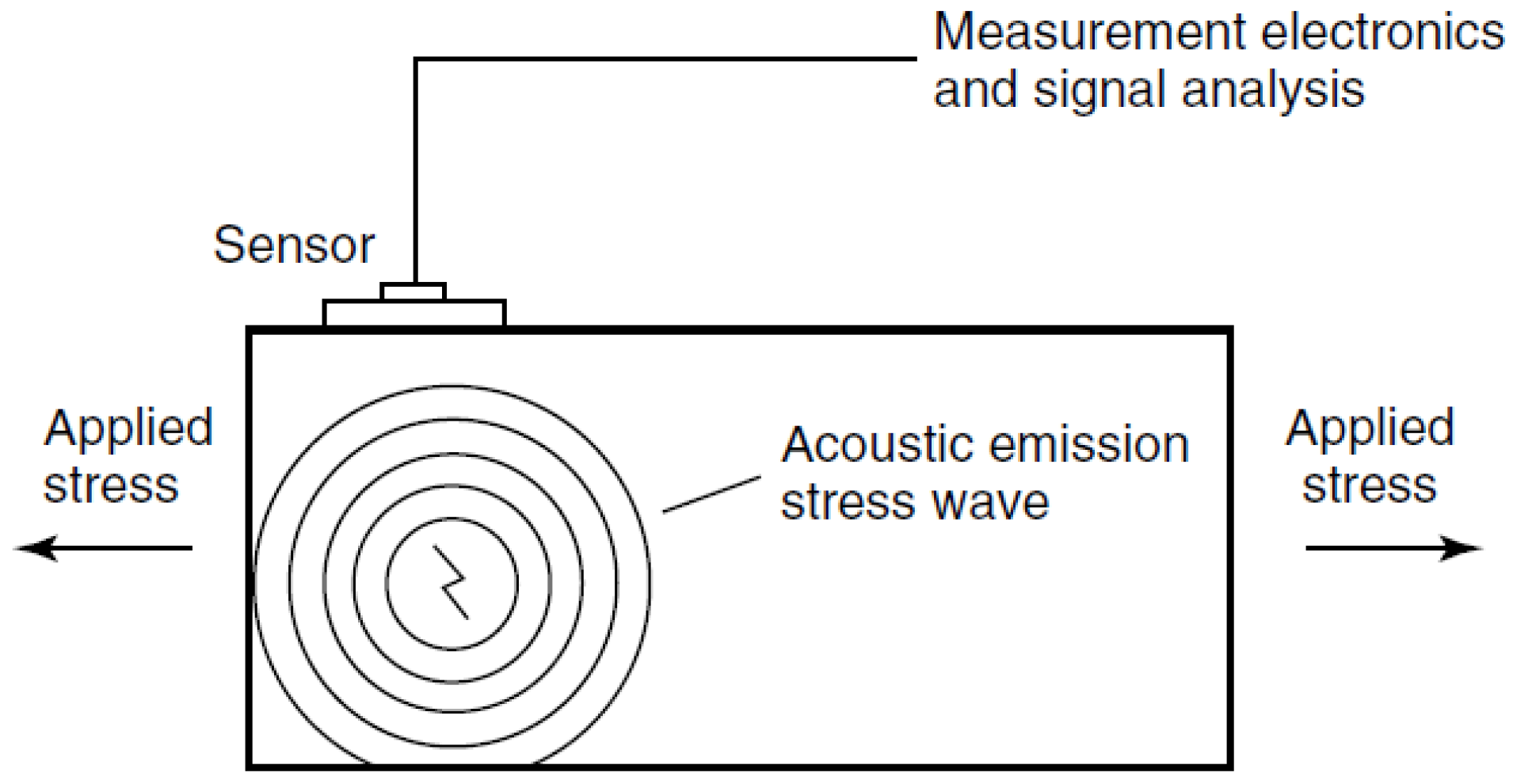
When an abrupt structural change occurs in a small part of a solid (i.e., a dislocation, a crack initiation or growth, etc.) a sudden change in the stress/strain state happens in the small area where the change is produced. The small volume of material that is stressed releases its energy and produces a high-frequency vibration. This vibration propagates through the material producing an elastic wave that may be detected using a suitable transducer when it reaches the surface (Figure 1). This phenomenon is called acoustic emission (AE), and it is very useful because it permits the detection of structural changes in specimens (in laboratory tests) and in structures or parts (in operational service). In the first case, changes in the structure of the material can be studied with specific tests, and the strength can be quantified. In the second case, the premature failures of operating machines can be prevented [5].
The aim of this paper is to provide a review of the AE-based techniques for monitoring cavitation erosion and fatigue damage. The remaining sections of the paper are organized as follows: Section 2 presents the AE and its applications, Section 3 and Section 4 review the uses of AE for cavitation erosion and fatigue crack detection, respectively, Section 5 presents a discussion, and finally, Section 6 summarises the conclusions and the future work.
2. Acoustic Emission
The phenomenon of AE was first observed as audible sounds when materials were deformed. Already in the eighth century, the Arabian alchemist Jabir ibn Hayyan (also known as Gerber) wrote that Jupiter (tin) gives off a “harsh sound” or “crashing noise”, referring to an audible emission produced by the twinning of pure tin during its plastic deformation. Gerber also described that Mars (iron) makes a louder sound during forging. This sound was produced by the formation of martensite during the cooling process [6]. Joseph Kaiser conducted the first comprehensive study into the phenomena of AE [7]. The most significant discovery of Kaiser’s work was the irreversibility phenomenon that now bears his name, the Kaiser effect: if a material is loaded, it will emit some AE signals, but if it is unloaded and later reloaded, it will not emit any AE signal until the maximum charge level from before is reached. AEs are currently used in many areas of research, quality control and industry in general. AEs have been used in the study of different materials: metals [8,9,10,11,12,13], composites [14,15], additive manufactured materials [16] and human and other living being tissues [17,18]. Other applications are real-time leak detection and localisation [19,20], tool-wear monitoring and other studies on machining processes [21,22,23,24], the health monitoring of large structures [25,26], the study of cavitation and its erosion and the monitoring of fatigue crack onset and growth. The review of these last two applications constitutes the scope of this paper.
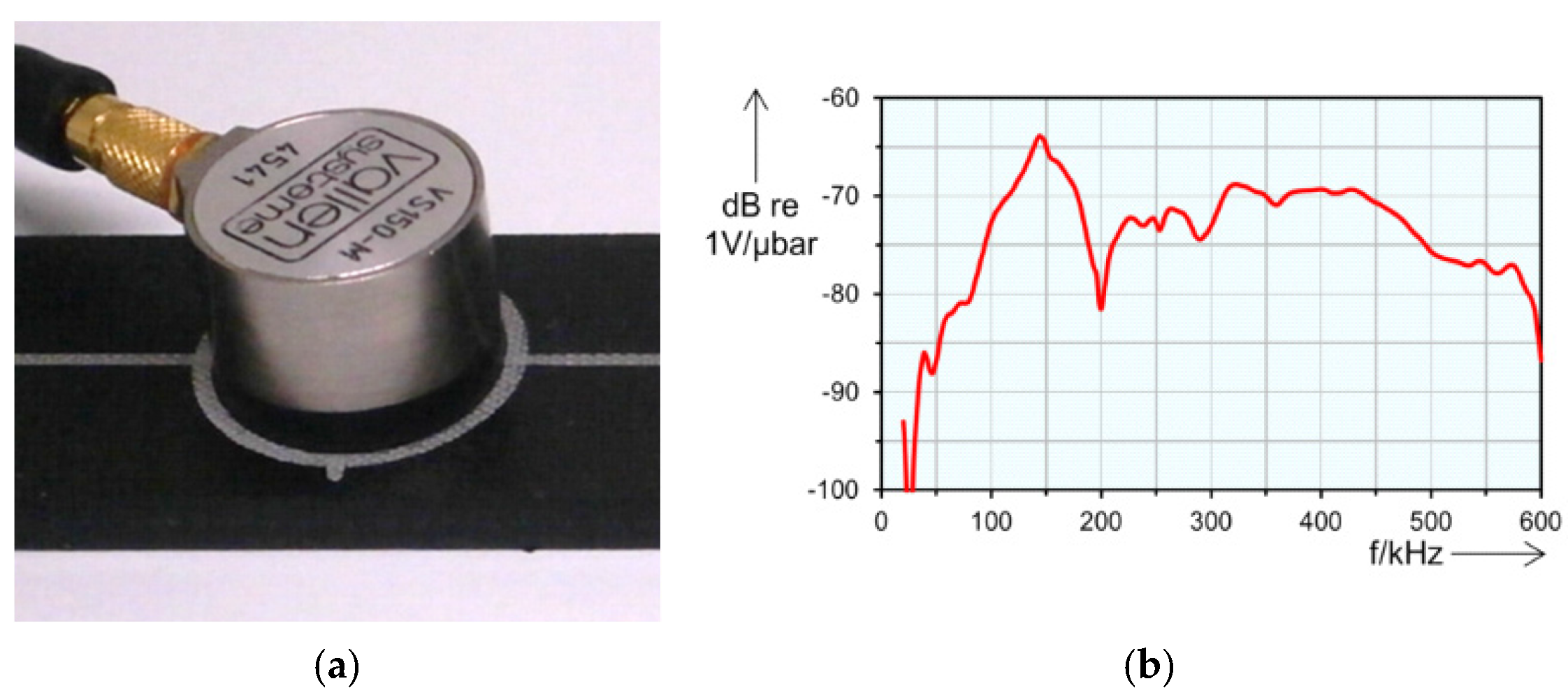
The elastic waves produced by an AE propagate inside the material and can be captured using a suitable sensor attached on the surface at the time the waves reach the surface. A contact type sensor is normally used in AE measurements, such as the one shown in Figure 2a. In most of the cases, a piezoelectric crystal enclosed inside a protective housing is employed as an AE transducer. These sensors are exclusively based on the piezoelectric effect out of lead zirconate titanate (PZT). AE signals are detected in the form of dynamic motions over the surface of a material, and they are converted into electrical signals using a PZT piezoelectric transducer [27]. In contrast to accelerometers, the frequency response function (FRF) of a PZT AE sensor presents a significant deviation from a preferred flat frequency response due to the proximity between the PZT natural frequencies and the characteristic elastic wave frequencies. Thus, the sensitivity of an AE sensor depends on the frequency. Additionally, unlike accelerometers, which are carefully designed to measure only the motion component parallel to their axis, AE sensors respond to motions in any direction [28]. Figure 2b shows the FRF of an AE sensor. Sensors of different models have different FRFs. Consequently, if different AE signals are to be compared, they shall be measured with the same sensor model.
Typical data acquisition schemes for AE measurements comprise both amplification and filtering stages. Amplifiers boost the signal voltage to bring it to a level that is optimal for the measurement stage. Along with several stages of amplification, frequency filters are incorporated into the AE measurement chain. These filters define the frequency range to be used and attenuate low frequency background noise. This process of amplification and filtering is called “signal conditioning”. It “cleans” the signal and prepares it for processing. After conditioning, the signal is digitalised for its recording or/and processing. Sampling frequencies must be very high (of the order of MHz) because of the high frequencies of AE signals [27].
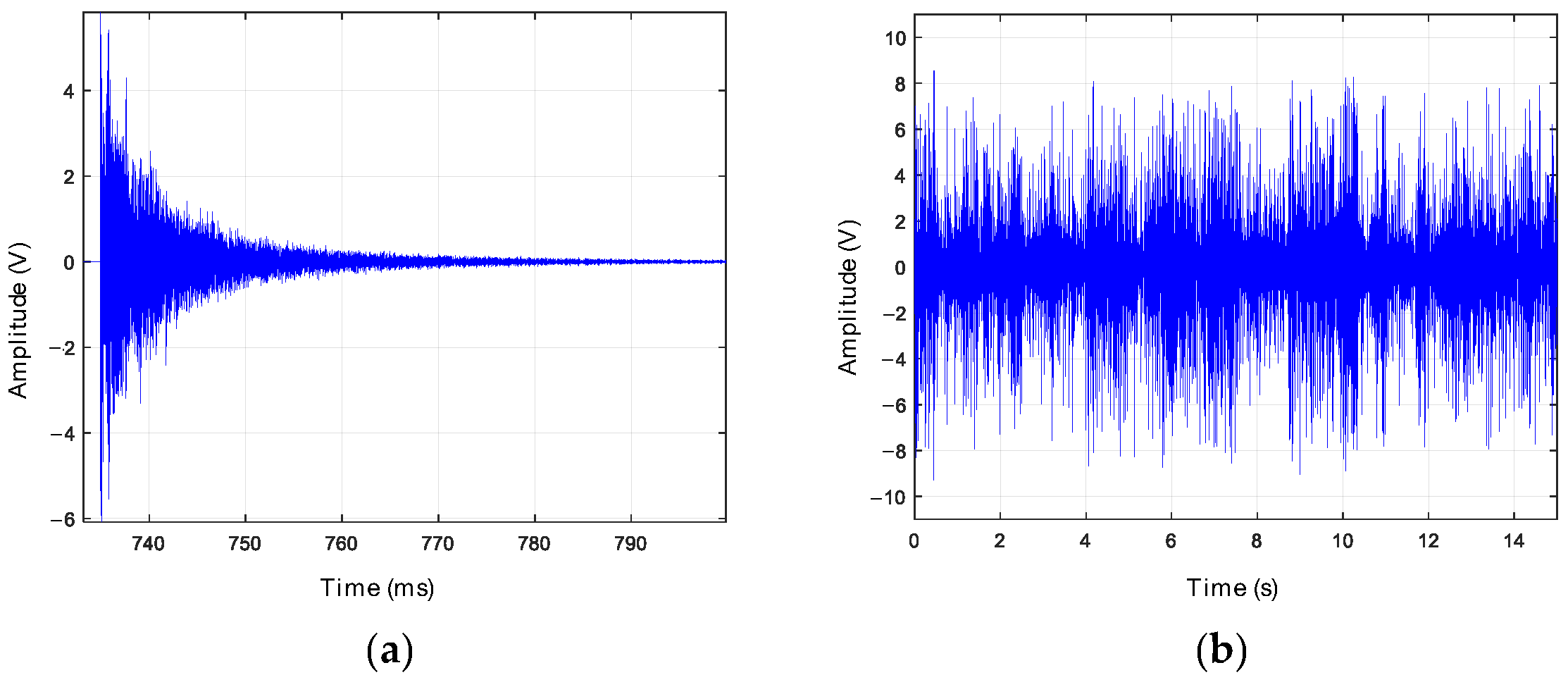
AE signals can be classified into two general classes: burst signals and continuous signals. Burst signals have a clearly defined start and end relative to background noise, and thus, they have a well-defined duration (Figure 3a). A burst signal, from its beginning to its end, is also called a hit. On the other hand, continuous signals, although they present variations in their amplitude and frequency over time, do not have a defined beginning and end, and they are maintained as long as the process that generates them is active (Figure 3b).
Approaches for analysing AE signals can be divided in two groups: parameter-based analysis and signal-based analysis. In the first approach, as the signal is acquired, the characteristic parameters that describe the waveforms of the different parts of the signal (hits) are computed, and even the whole hit can be recorded; thus, parameter-based analysis can be used with burst signals only. This is usually an on-line processing. In a signal-based analysis approach, the raw signal is usually recorded for further analysis. It can be used with burst and continuous signals [27].
2.1. Parameter-Based Analysis
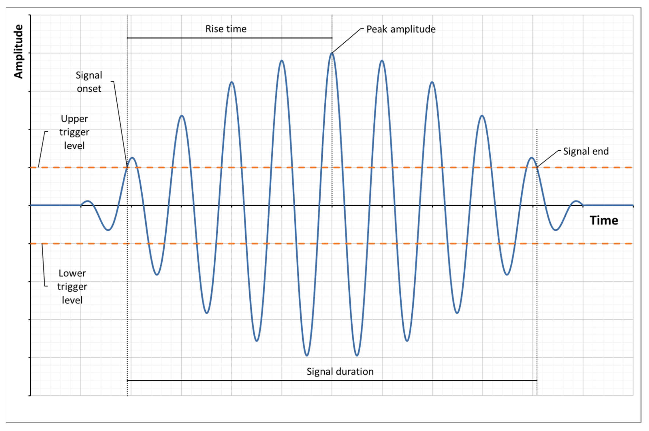
Burst signals have to be clearly defined relative to the background noise. In order to detect burst signals, it is necessary to have previously set a threshold amplitude level above the background noise. In Figure 4, the main parameters of a characteristic AE time-response signal are presented. The burst signal onset is defined as the instant at which the absolute voltage exceeds the predetermined threshold level. It is considered that the burst signal has ended when a determined time, called the Hit Lockout Time, has passed without any further signal crossing the threshold [30]. The burst signal from its onset to its end is called a hit.
Parameter analysis is based in the extraction of descriptors that contain most of the waveform information, which are the following ones (Figure 4) [30]:
- Counts are the number of times within the signal that the AE amplitude reaches the threshold level. For example, this number is 7 in Figure 4.
- Amplitude is the peak voltage of the signal waveform, which can be positive or negative. Amplitudes are expressed in decibels on a logarithmic scale. Commonly, 1 μV is defined as 0 dB AE.
- Energy is generally defined as a Measured Area under the Rectified Signal Envelope (MARSE). While this is an “engineering” value, another definition of energy, known as “absolute energy”, is computed as the integration of the rectified squared waveform. It is considered analogous to the actual energy released from the AE source:
Duration is the time interval between the first count and the last descending threshold crossing.
Some parameters can be calculated from the hit-frequency spectrum. The most remarkable ones are the peak frequency and the centroid frequency:
- The peak frequency is the frequency corresponding to the highest magnitude in the spectrum.
- The centroid frequency is given by the following expression:
2.2. Signal-Based Analysis
In this subsection, several approaches that consider the entire AE waveform are described. The basic premise is that the AE waveforms are recorded, and their changes over time are characterised and interpreted [31]. Different analyses can be conducted, such as those presented in the following subsections.
2.2.1. Frequency Analysis
Frequency analysis techniques are widely used, ranging from simple filtering to more sophisticated approaches. AE signals can be filtered with a high-pass filter in order to remove the low-frequency background noise [31]. Furthermore, signals can be demodulated using the Hilbert transform [32], such as in cavitation analyses, in order to identify the characteristic frequencies of its dynamic behaviour [33].
2.2.2. Time–Frequency Analysis
This family of techniques is well suited for non-stationary signals and includes the wavelet transform (WT) and the short-time Fourier transform (STFT). An advantage of these techniques is that they are able to relate changes in the frequency characteristics of the signal within the time domain [31]. Both techniques can also be used as a signal conditioning stage to improve denoising. These transforms produce tri-axis diagrams (X-time, Y-frequency and Z-amplitude) that are plotted in colour-scaled plots called spectrograms.
Although the WT shows a good performance for processing signals in the time–frequency domain, its application requires the selection of a suitable wavelet function before the analysis. As different wavelet functions result in different output results, the Empirical Mode Decomposition (EMD) method was introduced in 1998 [34] to reduce the impact of a pre-defined wavelet function. EMD decomposes any complex dataset into a finite number of Intrinsic Mode Functions (IMFs) that provide information about instantaneous frequency and energy instead of the global pictures defined by the Fourier spectral analysis [35,36]. Enhanced Empirical Mode Decomposition (EEMD) is a refinement of EMD used to overcome a mode-mixing problem that appears with intermittent components [37]. In EEMD, the mode-mixing problem is removed by adding white noise to the processed signal. Lei et al. [38] have compared decomposed signals using both methods and concluding that EEMD is more accurate than EMD. Complete EEMD (CEEMD) is a further refinement wherein the decomposition provides a more accurate reconstruction of the original data [39].
2.2.3. Machine Learning Approaches
Pattern recognition and clustering have been proposed to discriminate different types of AE events. The goal is that waveforms with similar features are grouped (or clustered), corresponding to different source mechanisms or failure types. A set of characteristics, or parameters, are deducted from each type of signal, which is then considered by the algorithm to determine the clusters. Different machine learning algorithms are used with AE signals. The k-nearest neighbour algorithm (k-NN) is one of the simplest ones: the output value of any test point is the average of the k-nearest output values from the training distribution [31]. The random decision forest (RF) is an ensemble learning algorithm for regression problems that constructs a robust number of decision trees during training, and the average prediction value of the training trees is returned as the final predicted result [40]. The support vector machine (SVM) is an algorithm that constructs a hyperplane with the shortest possible distance between it and the sample points. It has exhibited a good generalisation capability and high prediction accuracy in cases of limited training datasets [41].
Neural networks (NNs) consist of an input and output layers that are connected through a number of hidden layers, all mathematically related via non-linear relationships that must be estimated (learning) [30]. Convolutional neural networks (CNNs) are defined as NNs that use the convolutional operation, which is defined as the dot product between a grid-structured set of numbers (weights) and similar grid-structured inputs drawn from different spatial locations in the input [42]. CNNs are commonly used in image recognition processes. For example, Gaisser et al. [43] employed spectrograms of AE signals measured in hydraulic turbines as the input of a CNN to detect cavitation.
3. Cavitation Detection and Erosion Prediction
When the static pressure of a liquid drops below its vapor pressure, part of the liquid evaporates and forms vapor-filled bubbles. When the pressure rises again above the vapor pressure, vapor condenses, and the bubbles (or cavities) collapse. As a result, shock waves and high-velocity micro-jets collide against the nearest solid walls, producing very high local pressures that can reach up to 700 MPa [44], which result in damage (pitting). The successive repetitions of these impacts produce an aging of the material, and, finally, small parts of it are detached, thus showing the start of the material erosion (mass loss).
In hydraulic turbines, the static pressure of water varies as it flows through the conduits and the runner, making it prone to cavitation. The most affected turbine parts by cavitation are the runner and the draft tube cone [44]. As explained in Section 1, hydraulic turbines often run in off-design operation mode, far from their BEP. This increases the probability of cavitation inducing erosion. Therefore, it is necessary to detect cavitation in hydraulic turbines and to predict the cavitation erosion to schedule preventive maintenance and to avoid catastrophic failures. The measurements of vibrations, AEs, dynamic pressures and noise are commonly carried out to detect the presence of cavitation and to predict erosion.
The cavitation research is mainly focused on two aspects [45]: experimental measurements and computational fluid dynamic (CFD) simulations. The latter has gradually become an important method used to explore and understand the internal flow behaviour of hydraulic machines [46]. The former includes many techniques such as the measurement of the main effects of cavitation (vibrations, AEs, noise and dynamic pressures), flow visualisations with high-speed cameras [47], particle image velocimetry (PIV) and laser Doppler velocimetry (LDV), among others. Experimental studies can be carried out in the laboratory with reduced-scale model turbines machines or cavitation tunnels, or in full-scale prototype turbines located in hydropower plants. It is worth it to note that invasive methods and flow visualisation techniques cannot be easily used on prototype turbines because it is necessary to ensure access to the internal components with the machine stopped and to install transparent windows. Thus, research on cavitation in prototype turbines has been mainly based on the external measurement of the effects of cavitation with traditional sensors. The use of vibrations, dynamic pressures and noise signals has also been considered in this review because all of them share similar analysis procedures to the ones used with the AE signals.
Avellan et al. [48] studied, in 1988, cavitation on a two-dimensional hydrofoil installed in the test section of a high-speed cavitation tunnel. They found that cavitation erosion results from the collapse of swirling transient vortices originated at the leading edge. These vortices are shed away of the closure region of the sheet cavity at a defined shedding frequency [49]. In hydraulic machines, this shedding frequency is governed by the cavitation interaction with the induced flow instabilities, which can be generated by the passage of blades in front of the wakes of the guide vanes and the spiral case tongue or by a draft tube swirling flow starting at the runner hub (outlet swirl). Then, the shedding frequency is forced to a frequency characteristic to the particular design of each machine corresponding to the blade passing frequency, the guide vane frequency or the swirl frequency [50]. Thus, a signal measured on a machine suffering cavitation will be modulated by the corresponding shedding frequency (or frequencies), which can be identified by an amplitude demodulation process. Different procedures have been used to demodulate these signals: full-wave rectification using electronic circuits [50,51,52], Hilbert transform [33,53] and spline interpolation over local maximums [54]. Previously to the demodulation process, a passband filter has to be applied, usually located in a high-frequency band of the order of kHz.
Abbot et al. studied cavitation in a high-speed cavitation tunnel [51] and in different turbines [52]. Demodulation was carried out through the full-wave rectification of accelerations previously bandpass filtered from 10 to 20 kHz. Kaye et al. used high-frequency vibrations for different cavitation studies on turbines [50,53]. In Kaye et al.’s study [53], vibrations were acquired on several guide vanes and on the turbine guide bearing of a Francis turbine prototype that were then demodulated using a bandpass filter from 80 to 100 kHz, and the envelope was determined using the Hilbert transform. The analysis of the processed signal showed a well-defined peak at the blade passing frequency and a wide spread of values, indicating that the cavitation was very unstable. In Kaye et al.’s study [49], vibrations filtered from 40 to 50 kHz were acquired on the guide bearings and above two guide vanes. The demodulation envelope was determined using an analogue demodulator previous to the data acquisition, which allowed the use of a low sampling frequency and the acquisition of long-time signals containing many rotations of the turbine shaft. The envelope signals were processed in the frequency domain, showing the characteristic peak frequencies of the cavitation, and in the time–frequency domain using a spectrogram (STFT), showing the stability of these particular frequency peaks.
Escaler et al. [32] studied cavitation in several turbines using vibrations, dynamic pressures and AEs. The signals were bandpass filtered and demodulated using the Hilbert transform. In the case of two turbines suffering inlet leading edge cavitation, vibrations and AEs were measured on the bearing and guide vanes at different output loads. The frequency spectra showed a clear amplitude increase in a wide frequency band with the output load. Moreover, the blade and guide vane passing frequencies were identified in the spectra of the demodulated signals. In the case of a reduced-scale model of a Francis turbine, various analysis were performed at the BEP and at higher loads. The frequency spectra of bearing vibrations showed that the levels in all frequency bands increased as the flow rate increased. The demodulated spectra of the draft tube cone vibrations and pressures showed the blade passing frequency and its second harmonic. Finally, two prototype turbines suffering draft tube swirl were analysed. In a pump turbine, dynamic pressures were measured at the draft tube at 50, 75 and 100% of the output load. The spectrum at 50% load showed a maximum peak at a frequency equal to 0.31 times the turbine rotating frequency corresponding to the rotating vortex rope (RVR). In a Francis turbine, vibrations and AEs were measured on the guide bearing and on the guide vanes at different output loads. The spectra showed the amplitude increase in all the frequency bands with the load, and the spectra of the demodulated signals showed a frequency peak at 0.27 times the turbine rotating frequency at low loads (corresponding to the RVR) and at the guide vane passing frequency at high loads.
Table 1 shows a summary of the above-mentioned case studies. Despite the signal demodulation technique applied in the previously described references [33,50,52,53], it enables us to know if cavitation takes place, but it does not allow us to distinguish if the cavitation is erosive or not.
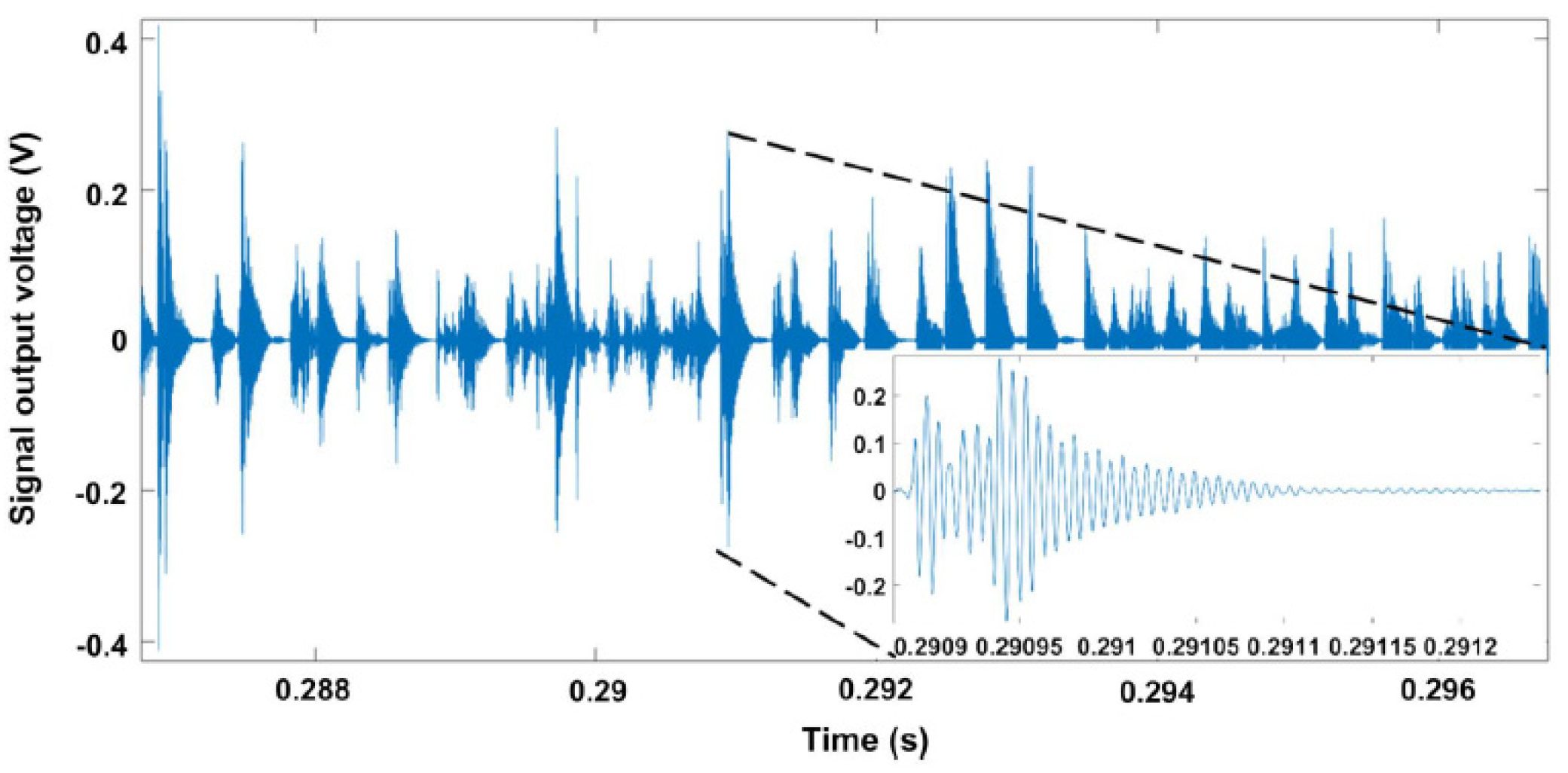
In the period 2018–2020, Ylönen et al. performed an extensive study on cavitation in a high-speed cavitation tunnel [55]. Polished stainless steel mirror samples were exposed to cavitation in periods of a few minutes in order to not exceed the incubation period, and, in parallel, an AE time signal was monitored [56]. Figure 5 shows an AE signal and a zoom in on one of the peaks measured during the cavitation incubation period [56]. The pits were measured using an optical profilometer, and the cavitation damage was characterised by the pit diameter distribution. The monitored AE signals were demodulated by fitting an envelope function calculated via spline interpolation over the local maxima in order to identify the hits in the signal and to determine their amplitudes [54]. A relationship between the cumulative distributions of the amplitude peak values and pit diameters was established. It was concluded that, in the incubation period, AE signal analysis can be used to monitor the deformation of pits without visual examination of the surface damage.
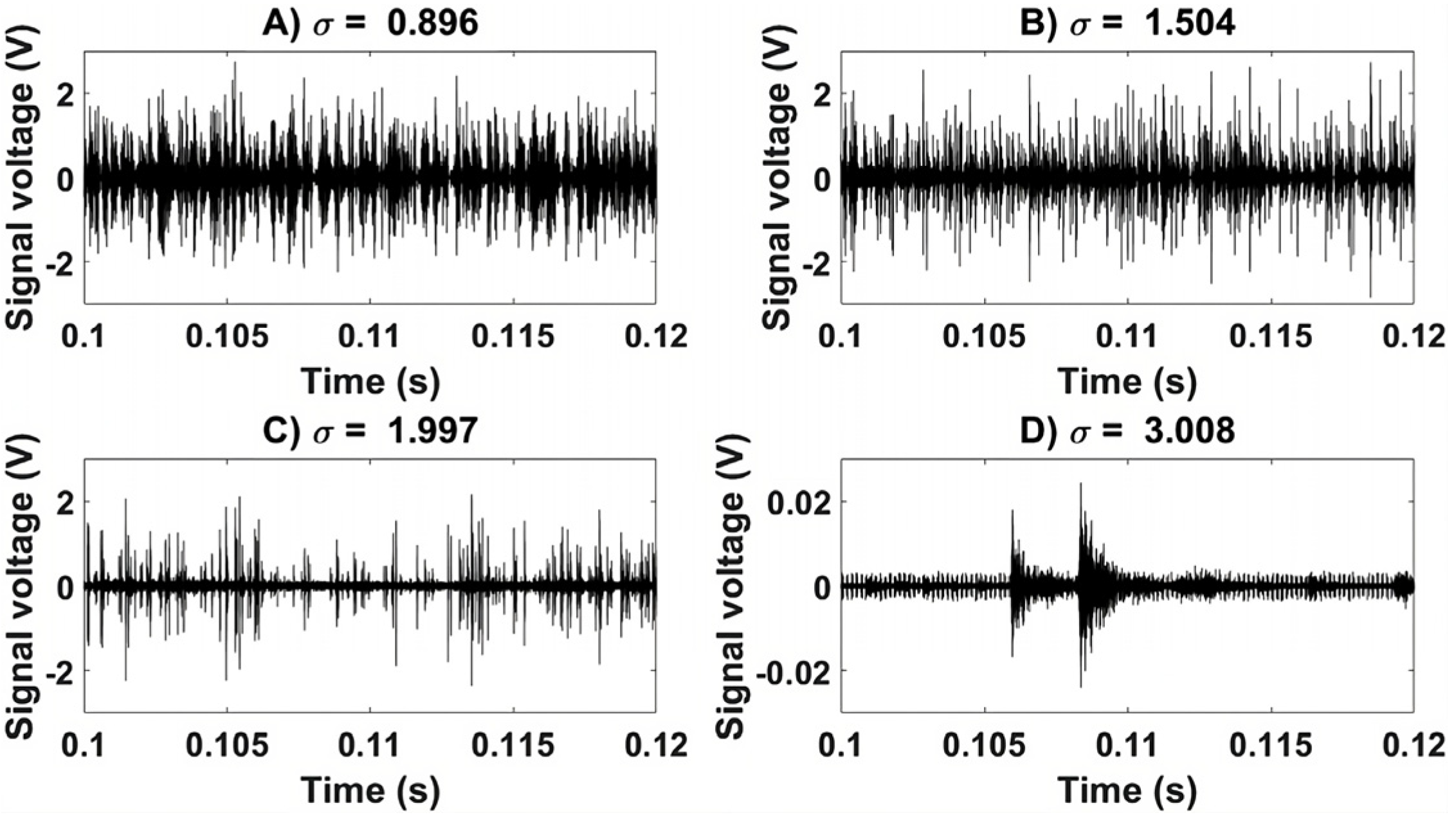
In order to study the possibility of monitoring the cavitation shedding frequency with AEs, ramp tests through a set of experimental conditions ranging from well-developed cavitation to no cavitation were performed in a high-speed cavitation tunnel. The monitored waveforms were demodulated, and the shedding frequencies were identified [57]. Non-dimensional cavitation numbers were related to shedding frequencies, and a relationship was observed. For cavitation numbers lower than 1.75, which corresponds to the cloud cavitation state, a linear trend between cavitation number and shedding frequency was observed, but for higher cavitation numbers and sheet cavitation onsets, the shedding frequencies were found to become unsteady. Hence, the point at which the shedding frequency appears unsteady can be used to detect the transition from cloud to sheet cavitation [57]. In order to study the relationship between shedding frequency and erosion, two stainless steel samples were eroded from a virgin non-eroded surface to an approximately 400 µm maximum erosion depth during 65 h of exposure to cloud cavitation. AEs were measured every one or two hours, and it was concluded that the shedding frequency increased when the volume loss and erosion depth also increased. It was also found that the increasing surface roughness leads to increases in the shedding frequency. The main conclusion was that these results could be used to track the erosion stage induced by cavitation on a hydrofoil in a cavitation tunnel [57]. Figure 6 shows the AE signals measured for different cavitation conditions: (A) and (B) correspond to fully developed cloud cavitation, (C) corresponds to sheet cavitation and (D) corresponds to cavitation-free conditions [57].
Recently, different methods for identifying the cavitation condition have been proposed based on artificial intelligence (AI). These methods employ AEs, vibrations, dynamic pressures and noise as inputs. Zhou et al. [58] developed a method to monitor the cavitation state in a Francis model turbine using AE signals for which their wavelet transform was introduced in a NN. The output of the developed method was the cavitation state: no-cavitation, primary cavitation, critical cavitation and severe cavitation. Tiwari et al. [59] developed a cavitation detection method for centrifugal pumps using the standard deviations, mean values, kurtosis and skewness values of dynamic pressures as the inputs of a two-layer NN that identified pump blockage and/or cavitation. Amini et al. [60] developed a cavitation detection methodology based on a Gaussian mixture model that classified turbine noise signals into cavitating and non-cavitating categories. The detection system was developed based on laboratory tests and validated in a hydropower plant.
Gaisser et al. [43] developed a CNN for cavitation detection that handled the data from different turbines (two Kaplan, two Francis and one Pump turbines), improving usual approaches that require learning on a specific machine. This approach creates a representation of the data and combines it with the domain-aligned training to generate a network to a variety of hydraulic machines. The training cavitation data stem from six model machines, and the testing data stem from five prototypes working in different powerplants. A cluster analysis was performed with AE data, and the result was that the data were clustered according to the machines instead of the class labels (cavitating conditions). This demonstrated that the differences between the machines were more dominant than the differences between the cavitating conditions. This is called a multi-source multi-target problem that can be solved with a special class of machine learning methods capable of dealing with multiple domain shifts. Then, a domain-alignment method for training deep NNs, called domain-adversarial training [61], was applied. With this approach, a framework for cavitation detection, which is applicable to a variety of hydraulic machinery, was successfully developed.
Table 2 shows a summary of the case studies discussed above.
In summary, erosive cavitation in hydraulic turbines can be detected measuring the induced effects from various quantities: AEs, vibrations, dynamic pressures and noise. Mainly two approaches have been developed based on amplitude demodulation and on AI. The former is based on the fact that the signals are modulated at the characteristic frequencies of the particular cavitation dynamic behaviour. The spectral content of the signal envelope in a high-frequency band provides this information, which indicates the location where cavitation occurs inside the hydraulic machine. Conversely, an accurate methodology for quantifying the amount of erosion caused by the cavitation has not been developed yet. Recently, AI has also been successfully used to detect cavitation. Nevertheless, there is no AI methodology able to detect whether cavitation is erosive or not, or in which part of the turbine it occurs.
4. Crack Detection Using Acoustic Emissions
Fatigue cracks are one of the predominant failure modes in hydraulic turbines. Fatigue damage starts with the initiation of cracks and continues with their propagation until an unstable size is reached that produces the breakdown of the component. AEs can be used to track this process of crack initiation and growth.
Dunegan et al. [62] presented a model that states that the cumulative AE counts (η) on a specimen in a tensile strength test are proportional to the fourth power of the stress intensity factor (K), as expressed by Equation (3):
In spite of that, some tests presented with aluminium and beryllium specimens in the same study exhibited a mechanical behaviour that differed significantly from the one predicted by the model, with experimental exponents higher than four.
Bassim [63] presented a relationship between the AE count rate () and the stress intensity factor range () in metallic materials, as expressed by Equation (4):
where is the number of fatigue cycles, is the stress intensity factor range, and and are material-dependent constants. This expression is similar to the Paris–Erdogan law [64], which, when combined with Equation (4), permits the derivation of a relationship between fatigue crack growth rate ( and for metallic materials, as given by Equation (5) [65,66,67]:
where a is the fatigue crack length, and m and s are material-dependent constants. This means that a can be estimated through the integration of , and a can be estimated without knowing the load-time history or complex calculations of . Roberts et al. [65] performed fatigue tests on specimens made from grade S275JR steel, with load ratios R of 0.1, 0.3 and 0.5 and the simultaneous measurement of AEs. Measuring only the counts among the top 10% of the applied range, they claimed that the prediction based on the above procedure exhibited a reasonably close correlation with the experimental results.
Yu et al. [68] developed a model that includes the acoustic energy rate, crack driving forces, fracture toughness and load ratio, as expressed in Equation (6):
where is the absolute energy change rate (based on AE data), is the load ratio, is the fracture toughness, is the high-stress intensity factor, and and are material-dependent constants.
Li et al. [69] developed a methodology for AE crack sizing based on bending tests on rail steel specimens for different load conditions. A classification index based on the wavelet power (WP) of the AE signal was first established to distinguish the crack closure-induced AE waves from the crack propagation-induced ones. Then, a method for crack sizing was developed based on the experimental finding that the crack closure-induced AE count rate correlates positively with crack length in the structure.
Pascoe et al. [70] used AEs to study crack growth behaviour during a single fatigue cycle using double cantilever beam specimens made of two aluminium Al2024-T3 arms bonded with Cytec FM-94 epoxy adhesive. A pre-crack was created along one edge of the double cantilever beams, and from a quasi-static test, it was concluded that the strain energy release ratio (SERR) calculated according to ASTM D3433-99 [71] was larger than the SERR at which the crack growth physically started. On the other hand, it was observed that the crack could grow during the loading and unloading phases of the load cycle during fatigue tests and that the crack growth did not occur just at maximum load or near the minimum load. Thus, the relevance of the maximum value and range of SERR used in many fracture mechanics formulas is in doubt. The interest of the cited study relays on the fact that the authors analysed the AE during a single fatigue cycle on bonded specimens, allowing the study of the behaviour of the glue. Referring to the authors’ conclusions, it might be assumed that all AE hits were produced by the crack extension, but they could also be produced by the crack closure, as it has been established in this review [69].
Joseph et al. [72] presented a method for correlating the AE signals produced by the fatigue crack growth with the crack length. It was observed that the generated AE energy resonated with the crack developing a steady wave pattern that depended on the crack length. A finite element model (FEM) was used to simulate a sensor and a crack with two length conditions (4 and 8 mm), which showed that the AE signal and its frequency spectrum depended on the crack length. These numerical results were verified through fatigue tests with aluminium 2024-T3 specimens using a novel stress-intensity factor-controlled fatigue crack growth method: fatigue loading was decreased as the crack grew in order to keep the stress-intensity factor constant [73]. Garrett et al. [74] introduced artificial intelligence to this procedure. AE hits corresponding to both crack lengths (in the ranges of 3.5–4.5 and 7.0–8.0 mm) were collected during the tests, and their wavelet transforms were computed and used as inputs in a CNN. Although this method is interesting from a theoretical point of view, its practical application seems now difficult. The relationship that the authors suggest depends on the shape of the piece or specimen, the material properties, the crack shape, the fracture mode (opening, sliding or tearing) and, probably, the location where the crack occurs. For all this, a lot of research is still needed for its practical application.
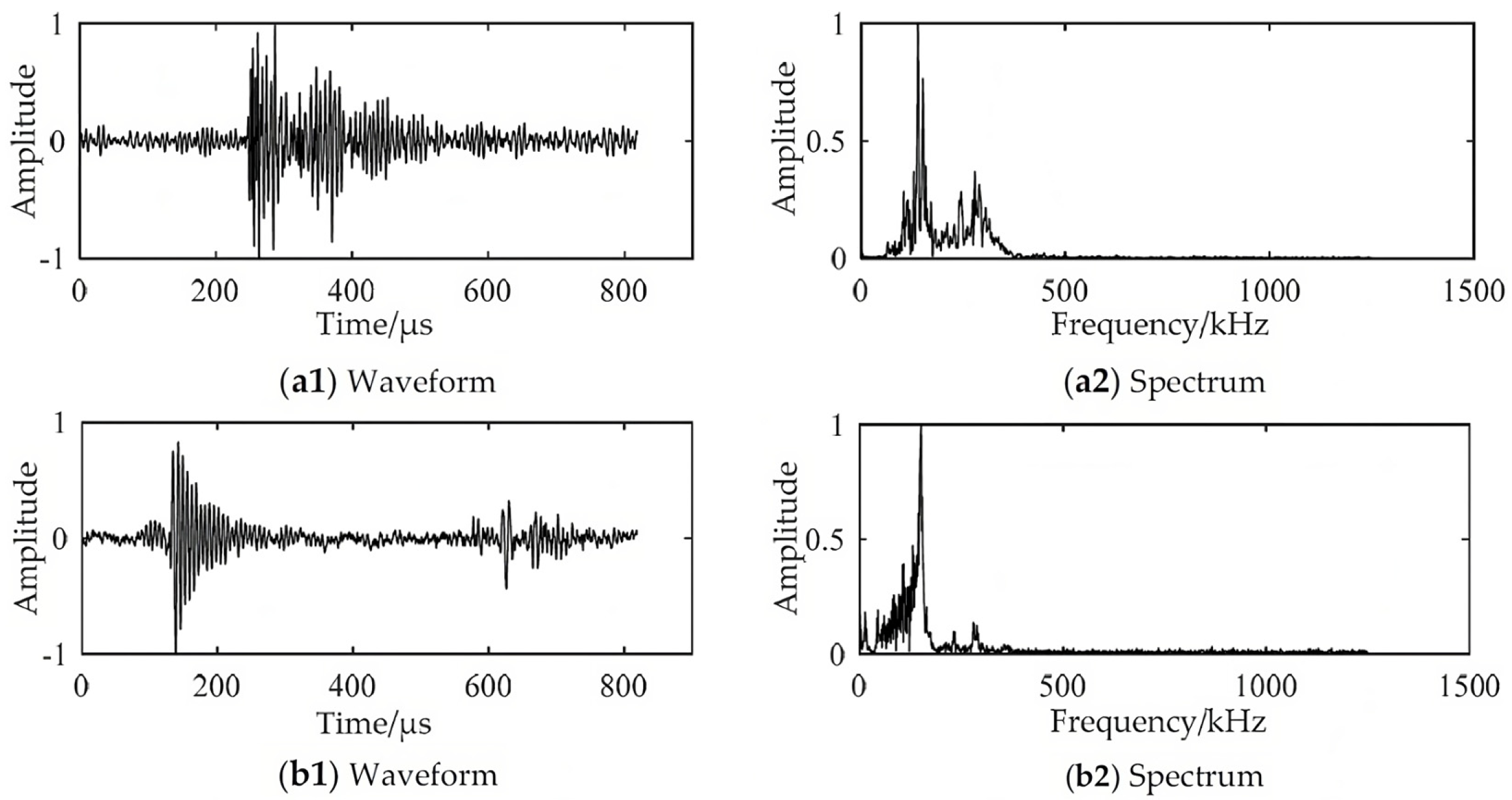
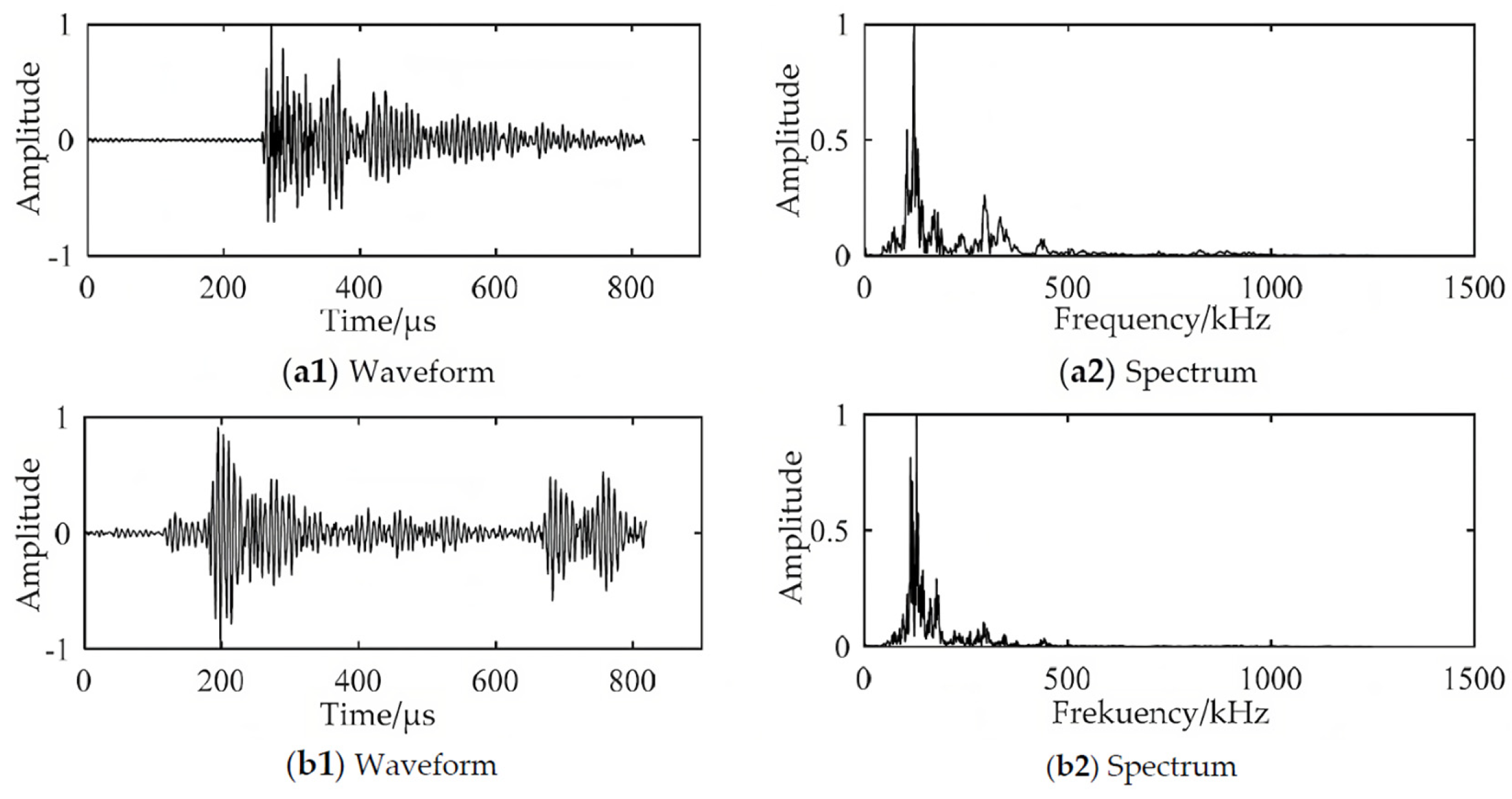
Zhang et al. [75] applied the AE technique to monitor the fatigue crack growth in two types of specimens: a gas turbine engine blade specimen and a TC11 titanium alloy plate specimen that is widely used in gas turbine engine blades. Based on the fracture mechanics and the experimental results, a mathematical model between the AE energy rate and crack growth rate was developed to predict the crack extension rate of the blade material and the residual fatigue life of the blades. Fatigue tests were carried out with both types of specimens, measuring AEs as well as the crack lengths along them. Two models of sensors were utilised with resonance frequencies of 125 kHz and 150 kHz. Figure 7 shows the AE signals and their spectra for the gas turbine engine blade specimen in two stages of the fatigue test: stable propagation stage (crack length of 2.5 mm) and fracture stage (crack length of 17.2 mm). Figure 8 shows the same kind of information corresponding to the TC11 titanium alloy specimen. This work did not indicate with which sensor model the measurements were carried out. Looking at the spectra of Figure 7 and Figure 8 and according to the frequency scale, the peak frequency could correspond to any of the two sensor frequencies (125 or 150 kHz).
Shiraiwa et al. [76] developed a method to classify the fatigue crack propagation in four stages that mainly correspond to the following: (i) microstructurally small crack growth, (ii) physically small crack growth, (iii) long crack propagation and iv) unstable crack growth. Fatigue tests with different specimens of different materials (pure iron, magnesium alloys and carbon steel) were performed, and the AEs were measured. From these measurements, different parameters were extracted: energy (), peak frequency (), rise angle () (rise time/amplitude), duration (), cumulative counts () and count rate (). All parameters were normalised between 0 and 1 using the minimum and maximum values measured in each test. The following crack growth model was proposed, as expressed with Equation (7):
where is an index of a stage in fatigue crack growth, is a coefficient, m is an exponent, and ε is the error (the difference between model results and measurements). The crack growth rate was also normalised between 0 and 1. C and m were defined to change stepwise at the transition points of the fatigue crack growth stages. The number of stages is a hyperparameter that was set to four for pure iron and magnesium alloys. For carbon steels, the number of stages was assigned to three because the specimens had a pre-crack that was considered to be equivalent to the first of the four stages. In order to determine the changing point of the fatigue crack growth stage using AE signals, a Bayesian analysis was applied to the proposed crack growth model. Markov chain Monte Carlo (MCMC) simulations with multiple changepoint models were applied to the proposed crack growth model. Under the assumption that the error value between the model and the observed crack growth rate fits on a normal distribution and the number of stages in the fatigue process is four (except for carbon steel specimens), the subsequent distribution of and were calculated using MCMC simulations. The fatigue crack growth was successfully divided into the four stages referred to above.
Chai et al. [77] studied the relationship between different AE parameters and fatigue crack growth. Bending fatigue tests on single edge notch specimens made from 316 LN stainless steel with different load ratios (0.1, 0.3 and 0.5), simultaneous AE acquisitions and crack length measurements were performed. Four time-domain parameters (peak amplitude, information entropy [78], energy and count) were extracted from the AE waveforms to characterise the fatigue damage. The relationships between the AE parameters and the fatigue crack growth rate on a log–log scale were established. In order to study the performances of different parameters in quantitatively describing the correlations between AE and fatigue crack growth, linear least squares regressions were performed to determine the model that best fit the observed data. The AE energy rate showed the best-fitting regression model results. The authors highlighted that the data points were obtained from AE waveforms recorded during the entire fatigue load cycle without any load-based AE data filtering procedure. The same authors proposed, in a further study [41] that was carried out with the results of the same tests, a back propagation NN model optimised with a genetic algorithm (GA-BPNN) for fatigue crack growth rate (FCGR) prediction. This model is based on AE parameters that can be ordered according to how significant they are relative to the FCGR prediction model. The AE energy rate was claimed again to be the feature that can provide the most accurate information for FCGR prediction in the current study. As stated before, they noted that the data points were obtained from AE waveforms recorded during the entire fatigue loading cycle without any load-based AE data filtering procedure. However, in reference [65], filtering was carried out, taking only the AE data corresponding to the top 10% maximum amplitudes of the applied range, as previously reported.
Referring to the crack initiation, Keshtgar et al. [79] proposed an intensity index of AE to detect crack initiation in 7075-T6 aluminium alloy. The intensity index encompasses the total value of weighted features including count, amplitude and rise time. It was discussed that the first detected jump (more than a 50% sudden increase) in intensity of AE signals with a relatively fast rise time and high amplitude, as well as high count numbers, corresponded to the crack initiation.
Vanniamparambil et al. [80] studied the AE produced by crack initiation in Aluminium 2024 Alloy specimens. They performed quasi-static and fatigue tests with the simultaneous recording of AEs, digital image correlation and infrared thermography. From these tests, they concluded that before crack initiation, AE waveforms were of a low-frequency continuous type due to the plastic strain, but that the waveforms became of high-frequency (534 kHz) and burst type from the onset of cracking. The authors proposed that this could be an indicator used to detect crack onset in metallic specimens, although they recognised that its validity at various distances from the source had to be assessed.
Karimian et al. [81] developed a method for detecting fatigue crack initiation in aluminium alloy using an information entropy AE parameter [77]. Some fatigue tests of different AA7075-T6 material notched specimens with different loading conditions were performed with simultaneous AE measurements. These tests were paused once a crack became visible. Only signals received in the top 20% of the peak load were considered to be related to fatigue damage. Then, the detected crack was measured, and the crack initiation cycle was calculated using the crack length at the termination cycle and material properties used in monotonic tests. The AE counts, energy and information entropy were calculated and analysed. The latter presented a minimum value just before the initiation of the crack, followed by a sudden increase in the accumulated entropy. This circumstance enables the instant (and number of cycles) in which the crack was initiated to be known.
Referring to the studies on hydraulic turbines, Wang et al. [82] compared AE signals obtained during a laboratory fatigue test with signals recorded in a hydropower plant. AE parameters were extracted from waveforms recorded during fatigue tests of different 20SiMn steel (material used for hydraulic turbine blades) specimens with simultaneous crack length measurements and during hydraulic turbine operation, and it was observed that they were very different. The background noise was found to be a continuous vibration signal, which had a longer duration, lower frequency range and higher amplitude. It might be noted that both tests should have been performed with the same AE sensor model; otherwise, the signals might not be comparable as a consequence of the different sensitivity of both sensors to the different frequencies. They also evaluated the attenuation characteristics at the propagation distances of the AE signals using a wavelet packet transformation [83] and also developed a procedure to locate cracks in a runner based on support vector machines [84]. Both works were carried out in laboratory conditions on a Francis turbine runner, and the AE signals were generated by braking pencil lead [85].
In summary, crack growth of metallic materials has been characterised in different ways with AEs: (i) relationships between K and different AE parameters (counts or energy) combined with the Paris–Erdogan’s law [64] have permitted the derivation of correlations with that do not require very complex computations; (ii) AE time and frequency parameters have been used to detect crack initiation; and (iii) wavelet power [69] or a relationship between hit spectrum and crack length [72] have permitted the estimation of the crack length. In addition, it is worth it to note the works of Pascoe et al. [70], who studied AEs during a single fatigue cycle, and of Shiraiwa et al. [76], who developed a procedure based on AEs that allows us to know the fatigue crack propagation stage. And finally, it has been found that AI is becoming a popular methodology for the crack characterisation of metallic materials, as demonstrated by the works of Garrett et al. [74], who studied crack length with AE hits using a CNN model, and Chai et al. [41], who developed a NN model optimised with a genetic algorithm to predict the crack growth from AEs. Unfortunately, only a few works have been conducted in laboratory conditions [82], or the crack growth has been simulated by breaking pencil lead on runners in studies on crack localisation [84] and AE transmission [83] in hydraulic turbines.
5. Discussion
The reviewed literature shows that fatigue damage (crack initiation or growth) can be detected through a signal analysis of the AEs. In addition, cavitation can be also detected with AEs using demodulation or AI methods. But cavitation can also be detected using other quantities like vibrations, dynamic pressures and noise. This suggests that while the AEs used to detect fatigue are directly related to the damage itself in the case of the fracture, the AEs used to detect the cavitation are induced by the hydrodynamic (dynamic pressure) or structural disturbances (vibrations, AEs, noise) generated by the cavitation phenomenon. Actually, it seems that in these cases, the AE sensor is used as a “high-frequency accelerometer”.
The present review has exposed that nowadays, it is not possible to use AEs to detect if the cavitation in hydraulic machinery is erosive or to quantify its erosiveness. The only exception is the correlation found between pit diameters and AE transient amplitudes in a high-speed cavitation tunnel by Ylönen et al. [56]. The pit diameters were related to the maximum amplitudes of the AE signals in the incubation phase [56], and a relationship between the shedding frequency and the material loss in the erosion phase was described [57]. Unfortunately, this relationship cannot be used in hydraulic turbines because the shedding frequency is forced by the rotor–stator interaction between the fixed guide vanes and the rotating blades or the swirl at the outlet of the runner [50]. Recently, the hydropower community witnessed a prominent growth in AI, as it has been described in Section 3. It must be noted that, among the studied turbines with the traditional demodulation method, AEs have been used only in one of them (14%). And among the studied turbines with AI, AEs have been used only in two of them (66%). This suggests that AI methods and AEs constitute a promising combination in the field of cavitation research but still need additional efforts. Cavitation detection is a well-developed technology, both in the laboratory and in the field, but nowadays, it is not possible to evaluate the possible damage that this detected cavitation produces. AI methods have been well incorporated into this technology, but more research should be conducted to identify and distinguish cavitation signals produced during the incubation phase (when plastic deformations are produced) and the erosion phase (when fractures are produced). Nonetheless, the spectra generated by these phenomena are expected to show measurable differences that will allow this characterisation.
Cracks of metallic materials have been characterised during fatigue tests using AEs, as presented in Section 4. Three main approaches have been identified: crack growth evaluation, crack initiation detection and crack length evaluation. Additionally, two evaluation cases have been found corresponding to the assessment of the AEs emitted during a single fatigue cycle with a bonded specimen, and to the estimation of the crack growth stage from the AEs emitted during a fatigue test. Moreover, the use of AI methods is growing in the metallic material crack characterisation field. In relation to hydraulic turbines, three studies have been reviewed corresponding to one laboratory research [82], as well as two studies on runners wherein the emitted AEs were generated by breaking pencil lead [83,84], but no applications have been found in actual prototypes. The detection of fractures with AEs is a well-developed technology in well-controlled laboratory conditions, but, as far as the authors are aware, there is little work on crack monitoring in industrial applications.
6. Conclusions
The detection of cavitation with AEs is a well-developed technology in laboratory conditions and in full-scale hydraulic turbines. Nowadays, it is not possible to determine in actual machines if the cavitation is erosive. Therefore, it cannot be determined if the material is suffering the incubation phase (when only plastic deformations are produced) or if it is already in the advanced erosion phase (when mass loss is produced). In this sense, only a correlation between AEs and erosion has been obtained in a high-speed cavitation tunnel. Therefore, further work must be carried out toward the prediction of cavitation erosion with AEs.
The detection of fatigue cracks with AEs is a well-established technology in well-controlled laboratory conditions and specimens, but again, few works have been conducted in real applications with actual hydraulic turbines. Therefore, further work must be performed in order to extend this laboratory-demonstrated technology to actual industrial environments.
Various AI methodologies have been recently applied to both cavitation and crack detection with successful results using AEs; therefore, this constitutes a very promising line of research for improving the understanding and the prediction of the induced damages.
Author Contributions
Conceptualization, I.F.-O., D.B., X.A.-G. and X.E.; methodology, I.F.-O., D.B., X.A.-G. and X.E.; writing—original draft preparation, I.F.-O.; writing—review and editing, D.B., X.A.-G. and X.E.; supervision, X.A.-G. and X.E.; project administration, X.E. All authors have read and agreed to the published version of the manuscript.
Funding
This research received no external funding.
Data Availability Statement
Data is contained within the article.
Conflicts of Interest
The authors declare no conflict of interest.
References
- Tvaronaviciene, M.; Baublys, J.; Raudeliuniene, J.; Jatautaite, D. Global energy consumption peculiarities and energy sources: Role of renewables. In Energy Transformation towards Sustainability, 1st ed.; Tvaronaviciene, M., Slusarczyk, B., Eds.; Elsevier BV: Amsterdam, The Netherlands, 2020; pp. 1–49. [Google Scholar]
- Avesani, D.; Zanfei, A.; Di Marco, N.; Galletti, A.; Ravazzolo, F. Short-term hydropower optimization driven by innovative time-adapting. Appl. Energy 2023, 310, 118510. [Google Scholar] [CrossRef]
- Han, S.; He, M.; Zhao, Z.; Chen, D.; Xu, B.; Jurasz, J.; Liu, F.; Zheng, H. Overcoming the uncertainty and volatility of wind power: Day-ahead scheduling of hydro-wind hybrid power generation system by coordinating power regulation and frequency response flexibility. Appl. Energy 2023, 333, 120555. [Google Scholar] [CrossRef]
- Georgievskaiaa, E. Predictive analytics as a way to smart maintenance of hydraulic turbines. Procedia Struct. Integr. 2020, 28, 836–842. [Google Scholar] [CrossRef]
- Wevers, M.; Lambrighs, K. Applications of acoustic emission for SHM: A review. In Encyclopedia of Structural Health Monitoring; Boller, C., Ed.; John Wiley & Sons, Ltd.: Chichester, UK, 2009; pp. 1–13. [Google Scholar]
- Drouillard, T.F. A History of Acoustic Emission. J. Acoust. Emiss. 1976, 14, 1–34. [Google Scholar]
- Kaiser, J. Untersuchungen über das Auftreten von Geräuschen beim Zugversuch. Ph.D. Thesis, Technische Universität München, München, Germany, 1950. [Google Scholar]
- Martinez-Gonzalez, E.; Picas, I.; Casellas, D.; Romeu, J. Detection of rack nucleation and growth in tool steels using fracture tests and acoustic emission. Meccamica 2015, 50, 1155–1166. [Google Scholar] [CrossRef]
- Martinez-Gonzalez, E.; Ramirez, G.; Romeu, J.; Casellas, D. Damage induced by a spherical indentation test in tool steels detected by using acoustic emission technique. Exp. Mech. 2015, 55, 449–458. [Google Scholar] [CrossRef]
- Kietov, V.; Henschel, S.; Krügel, L. Study of dynamic crack formation in nodular cast iron using the acoustic emission technique. Eng. Fract. Mech. 2018, 188, 58–69. [Google Scholar] [CrossRef]
- Kietov, V.; Henschel, S.; Krüger, L. AE analysis of damage processes in cast iron and high-strength steel at different temperatures and loading rates. Eng. Fract. Mech. 2019, 210, 320–341. [Google Scholar] [CrossRef]
- Morgner, W.; Heyse, H. Uncommon cries of cast iron elucidated by acoustic emission analysis. J. Acoust. Emiss. 1986, 5, 45–49. [Google Scholar]
- Sjögren, T.; Svensson, I.L. Studying elastic deformation behaviour of cast irons by acoustic emission. Int. J. Cast Met. Res. 2005, 18, 249–256. [Google Scholar] [CrossRef]
- Dahmene, F.; Yaacoubi, S.; Mountassir, M.E. Acoustic emission of composites structures: Story, success, and challenges. Phys. Procedia 2015, 70, 599–603. [Google Scholar] [CrossRef]
- McCrory, J.P.; Al-Jumaili, S.K.; Crivelli, D.; Pearson, M.R.; Eaton, M.J.; Featherston, C.A.; Guagliano, M.; Holford, K.M.; Pullin, R. Damage classification in carbon fibre composites using acoustic emission: A comparison of three techniques. Compos. B Eng. 2015, 68, 424–430. [Google Scholar] [CrossRef]
- Adrover-Monserrat, B.; García-Vilana, S.; Sánchez-Molina, D.; Llumà, J.; Jerez-Mesa, R.; Martinez-Gonzalez, E.; Travieso-Rodriguez, J.A. Impact of printing orientation on inter and intra-layer bonds in 3D printed thermoplastic elastomers: A study using acoustic emission and tensile tests. Polymer 2023, 283, 126241. [Google Scholar] [CrossRef]
- Sánchez-Molina, D.; Martínez-González, E.; Velázquez-Ameijide, J.; Llumà, J.; Rebollo-Soria, M.; Arregui-Dalmases, C. A stochastic model for soft tissue failure using acoustic emission data. JMBBM 2015, 51, 328–336. [Google Scholar] [CrossRef] [PubMed]
- García-Vilana, S.; Sánchez-Molina, D.; Llumà, J.; Fernández-Osete, I.; Veláquez-Ameijide, J.; Martínez-González, E. A predictive model for fracture in human ribs based on in vitro acoustic emission data. Med. Phys. 2021, 48, 5540–5548. [Google Scholar] [CrossRef]
- Zhang, J.-L.; Guo, W.-X. Study on the characteristics of the leakage acoustic emission in cast iron pipe by xperiment. In Proceedings of the 2011 First International Conference on Instrumentation, Measurement, Computer, Communication and Control, Beijing, China, 21–23 October 2011. [Google Scholar]
- Li, S.; Song, Y.; Zhou, G. Leak detection of water distribution pipeline subject to failure of socket joint based on acoustic emission and pattern recognition. Measurement 2018, 115, 39–44. [Google Scholar] [CrossRef]
- Nikhare, C.P.; Conklin, C.; Loker, D.R. Understanding acoustic emission for different metal cutting machinery and operations. J. Manuf. Mater. Process. 2017, 1, 7. [Google Scholar] [CrossRef]
- Klocke, F.; Döbbeler, B.; Pullen, T.; Bergs, T. Acoustic emission signal source separation for a flank wear estimation of drilling tools. Procedia CIRP 2019, 79, 57–62. [Google Scholar] [CrossRef]
- Arslan, M.; Kamal, K.; Fahad, M.; Mathavan, S.; Khan, M.A. Automated machine tool prognostics for turning operation using acoustic emission and learning vector quantization. In Proceedings of the 5th International Conference on Control, Automation and Robotics (ICCAR), Beijing, China, 19–22 April 2019. [Google Scholar]
- Jerez-Mesa, R.; Travieso-Rodriguez, J.A.; Gomez-Gras, G.; Llumà-Fuentes, J. Development, characterization and test of an ultrasonic vibration-assisted ball burnishing tool. J. Mater. Process. Technol. 2018, 257, 203–212. [Google Scholar] [CrossRef]
- Megid, W.A.; Chainey, M.A.; Lebrun, P.; Hay, D.R. Monitoring fatigue cracks on eyebars of steel bridges using acoustic emission: A case study. Eng. Fract. Mech. 2019, 211, 198–208. [Google Scholar] [CrossRef]
- Tziavos, N.; Hermida, H.; Dirar, S.; Papaelias, M.; Metje, N.; Baniatopoulos, C. Structural health monitoring of grouted connections for offshore wind turbines by means of acoustic emission: An experimental study. Renew. Energ. 2020, 147, 130–140. [Google Scholar] [CrossRef]
- Ohtsu, M.; Aggelis, D.G. Sensors and Instruments. In Acoustic Emission Testing. Basics for Research–Applications in Engineering, 2nd ed.; Grosse, C.U., Ohtsu, M., Aggelis, D.G., Shiotani, T., Eds.; Springer Nature: Cham, Switzerland, 2022; pp. 21–44. [Google Scholar]
- Ciaburro, G.; Iannace, G. Machine-learning-based Mmethods for acoustic emission. Appl. Sci. 2022, 12, 10476. [Google Scholar] [CrossRef]
- Vallen GmbH. Available online: https://www.vallen.de/sensors/non-integrated-preamplifier-sensors/vs150-m-2/ (accessed on 20 November 2023).
- Aggelis, D.G.; Shiotani, T. Parameters Based AE Analysis. In Acoustic Emission Testing. Basics for Research–Applications, 2nd ed.; Grosse, C.U., Ohtsu, M., Aggelis, D.A., Shiotani, T., Eds.; Springer Nature: Cham, Switzerland, 2022; pp. 45–71. [Google Scholar]
- Schumacher, T.; Linzer, L.; Grosse, C.U. Signal-Based AE Analysis. In Acoustic Emission Testing. Basics for Research–Applications in Engineering, 2nd ed.; Grosse, C.U., Ohtsu, M., Aggelis, D.G., Shiotani, T., Eds.; Springer Nature: Cham, Switzerland, 2022; pp. 73–116. [Google Scholar]
- Bendat, J.S.; Piersol, A.G. Random Data, Analysis and Measurement Procedures, 4th ed.; Wiley: Hoboken, FL, USA, 2010. [Google Scholar]
- Escaler, X.; Egusquiza, E.; Farhad, M.; Avellan, F.; Coussirat, M. Detection of cavitation in hydraulic turbines. Mech. Syst. Signal Process 2006, 20, 983–1007. [Google Scholar] [CrossRef]
- Huang, N.E.; Shen, Z.; Long, S.R.; Wu, M.C.; Shih, H.H.; Zheng, Q.; Yen, N.C.; Tung, C.C.; Liu, H.H. The empirical mode decomposition and the Hilbert spectrum for nonlinear and non-stationary time series analysis. Proc. Math. Phys. Eng. Sci. 1998, 454, 903–995. [Google Scholar] [CrossRef]
- Barbosh, M.; Dunphy, K.; Sadhu, A. Acoustic emission-based damage localization using wavelet-assisted deep learning. J. Infrastruct. Syst. 2022, 3, 1–24. [Google Scholar] [CrossRef]
- Zhou, Y.; Lin, L.; Wang, D.; He, M.; He, D. A new method to classify railway vehicle axle fatigue crack AE signal. Appl. Acoust. 2018, 131, 174–185. [Google Scholar] [CrossRef]
- Wu, Z.; Huang, N.E. Ensemble empirical mode decomposition: A noise-assisted data analysis method. Adv. Adapt. Data Anal. 2009, 1, 1–41. [Google Scholar] [CrossRef]
- Lei, Y.; He, Z.; Zi, Y. Application of the EEMD method to rotor fault diagnosis of rotating machinery. Mech. Syst. Signal Process 2009, 23, 1327–1338. [Google Scholar] [CrossRef]
- Torres, M.E.; Colominas, M.A.; Schlotthauer, G.; Flandrin, P. A complete ensemble empirical mode decomposition with adaptive noise. In Proceedings of the IEEE International Conference on Acoustics, Speech and Signal (ICASSP), Prague, Czech Republic, 22–27 May 2011. [Google Scholar]
- Joshi, A.V. Machine Learning and Artificial Intelligence, 1st ed.; Springer: Cham, Switzerland, 2020; pp. 61–62. [Google Scholar]
- Chai, M.; Liu, P.; He, Y.; Han, Z.; Duan, Q.; Song, Y.; Zhang, Z. Machine learning-based approach for fatigue crack growth prediction using acoustic emission technique. Fatigue Fract. Eng. Mater. Struct. 2023, 46, 2784–2797. [Google Scholar] [CrossRef]
- Aggarwal, C.C. Neural Networks and Deep Learning, 1st ed.; Springer: Cham, Switzerland, 2019; pp. 315–371. [Google Scholar]
- Gaisser, L.; Kirschner, O.; Riedelbauch, S. Cavitation detection in hydraulic machinery by analyzing acoustic emissions under strong domain shifts using neural networks. Phys. Fluids 2023, 35, 027128. [Google Scholar] [CrossRef]
- Kumar, P.; Saini, R.P. Study of cavitation in hydro turbines—A review. Renew. Sust. Energ. Rev. 2010, 14, 374–383. [Google Scholar] [CrossRef]
- Wu, Y.; Guan, X.; Tao, R.; Xiao, R. Neural network-based analysis on the unusual peak of cavitation performance of a mixed flow pipeline pump. Iran. J. Sci. Technol.-Trans. Mech. 2023, 47, 1515–1533. [Google Scholar] [CrossRef]
- Geng, L.; Zhang, D.; Chen, J.; Escaler, X. Large-eddy simulation of cavitating tip leakage vortex structures and dynamics around a NACA0009 hydrofoil. J. Mar. Sci. Eng. 2021, 9, 1198. [Google Scholar] [CrossRef]
- Dular, M.; Stoffel, B.; Širok, B. Development of a cavitation erosion model. Wear 2006, 261, 642–655. [Google Scholar] [CrossRef]
- Avellan, F.; Dupont, P. Cavitation erosion on hydraulic machines: Generation and dynamics of erosive cavities. In Proceedings of the 14th IAHR Symposium in Hydraulic Machinery: Progress within Large and High Specific Energy Units, Throndheim, Norwegian, 20–23 June 1988. [Google Scholar]
- Bourdon, P.; Simoneau, R.; Avellan, F.; Farhad, M. Vibratory characteristics of erosive cavitation vortices downstream of a fixed leading edge cavity. In Proceedings of the 15th IAHR Symposium on Modern Technology in Hydraulic Energy Production, Belgrade, Serbia, 11–14 September 1990. [Google Scholar]
- Kaye, M.; Farhat, M. Classification of cavitation in hydraulic machines using vibration analysis. In Proceedings of the 21st IAHR Symposium of Hydraulic Machinery and Systems, Lausanne, Switzerland, 9–12 September 2002. [Google Scholar]
- Abbot, P.A.; Arndt, R.E.; Shanahan, T.B. Modulation noise analyses of cavitating hydrofoils. In Proceedings of the Bubble Noise and Cavitation Erosion in Fluid Systems, ASME, New Orleans, LA, USA, 28 November–3 December 1993. [Google Scholar]
- Abbot, P.A. Cavitation detection measurements on Francis and Kaplan Hydroturbines. In Proceedings of the International Symposium of Cavitation Noise and Erosion in Fluid Systems, ASME, New York, NY, USA, 10–15 December 1989. [Google Scholar]
- Kaye, M.; Dupont, P.; Escaler, X.; Avellan, F. Cavitation erosion monitoring of a prototype Francis turbine by vibration analysis. In Proceedings of the Third International Symposium on Cavitation, Grenoble, France, 7–10 April 1998. [Google Scholar]
- Ylönen, M.; Saarenrinne, P.; Miettinen, J.; Franc, J.P.; Fivel, V. Cavitation bubble collapse monitoring by acoustic emission in laboratory testing. In Proceedings of the 10th International Symposiunm on Cavitation, Baltimore, MD, USA, 14–16 May 2018. [Google Scholar]
- Ylönen, M. Cavitation Erosion Monitoring by Acoustic Emission. Ph.D. Thesis, Tampere University, Tampere, Finland, 2020. [Google Scholar]
- Ylönen, M.; Saarenrinne, P.; Miettinen, J.; Franc, J.P.; Fivel, M.; Laakso, J. Estimated cavitation pit distributions by acoustic emission. J. Hydraul. Eng. 2020, 146, 04019064. [Google Scholar] [CrossRef]
- Ylönen, M.; Franc, J.P.; Miettinen, J.; Saarenrinne, P.; Fivel, M. Shedding frequency in cavitation erosion evolution tracking. Int. J. Multiph. Flow 2019, 118, 141–149. [Google Scholar] [CrossRef]
- Zhou, Y.; Liu, Z.; Zou, S.; Zhang, X. Turbine cavitation state recognition based on BP neural network. In Proceedings of the International Conference on Robots & Intelligent System (ICRIS), Haikou, China, 15–16 June 2019. [Google Scholar]
- Tiwari, R.; Bordoloi, D.J.; Dewangan, A. Blockage and cavitation detection in centrifugal pumps from dynamic pressure signal using deep learning algorithm. Measurement 2021, 173, 08676. [Google Scholar] [CrossRef]
- Amini, A.; Pacot, O.; Voide, D.; Hasmatuchi, V.; Roduit, P.; Münch-Alligné, C. Development of a novel cavitation monitoring system for hydro turbines based on machine learning algorithms. In Proceedings of the IOP Conference Series: Earth and Environmental Science, Melbourne, Australia, 26–30 October 2022. [Google Scholar]
- Ganin, Y.; Ustiniva, E.; Ajakan, H.; Germain, P.; Larochelle, H.; Laviolette, F.; Marchand, M.; Lempitsky, V. Domain-Adversarial training of neural networks. J. Mach. Learn. Res. 2016, 17, 1–35. [Google Scholar]
- Dunegan, H.L.; Harris, D.O.; Tatro, C.A. Fracture analysis by use of acoustic emission. Eng. Fract. Mech. 1968, 1, 105–122. [Google Scholar] [CrossRef]
- Bassim, M.N. Assessment of fatigue damage with acoustic emission. J. Acoust. Emiss. 1985, 4, S224–S226. [Google Scholar]
- Paris, P.; Erdogan, F. A critical analysis of crack propagation laws. J. Basic Eng 1963, 85D, 528–534. [Google Scholar] [CrossRef]
- Roberts, T.M.; Talebzadeh, M. Fatigue life prediction based on crack propagation and acoustic emission count rates. J. Constr. Steel Res. 2003, 59, 679–694. [Google Scholar] [CrossRef]
- Rabiei, M.; Modarres, M. Quantitative methods for structural health management using in situ acoustic emission monitoring. Int. J. Fatigue 2013, 49, 81–89. [Google Scholar] [CrossRef]
- Han, Z.; Luo, H.; Sun, C.; Li, J.; Papaelias, M. Acoustic emission study of fatigue crack propagation in extruded AZ31 magnesium alloy. Mater. Sci. Eng. A 2014, 597, 270–278. [Google Scholar] [CrossRef]
- Yu, J.; Ziehl, P. Stable and unstable fatigue prediction for A572 structural steel using acoustic emission. J. Constr. Steel Res. 2012, 77, 173–179. [Google Scholar] [CrossRef]
- Li, D.; Kuang, K.S.C.; Koh, C.G. Fatigue crack sizing in rail steel using crack closure-induced acoustic emission waves. Meas. Sci. Technol. 2017, 28, 065601. [Google Scholar] [CrossRef]
- Pascoe, J.A.; Zarouchas, D.S.; Alderliesten, R.C.; Benedictus, R. Using acoustic emission to understand fatigue crack growth within a single load cycle. Eng. Fract. Mech. 2018, 194, 281–300. [Google Scholar] [CrossRef]
- ASTM D3433-99; Standard Test Method for Fracture Strength in Cleavage of Adhesives in Bonded Metal Joints. ASTM: Philadelphia, PA, USA, 2012.
- Joseph, R.; Mei, H.; Migot, A.; Giurgiutiu, V. Crack-length estimation for structural health monitoring using the high-frequency resonances excited by the energy release during fatigue-crack growth. Sensors 2021, 21, 4221. [Google Scholar] [CrossRef] [PubMed]
- Joseph, R. Acoustic Emission and Guided Wave Modeling and Experiments for Structural Health Monitoring and Non-Destructive Evaluation. Ph.D. Thesis, University of South Carolina, Columbia, SC, USA, 2020. [Google Scholar]
- Garrett, J.C.; Mei, H.; Giurgiutiu, V. An artificial intelligence approach to fatigue crack length estimation from acoustic emission waves in thin metallic plates. Appl. Sci. 2022, 12, 1372. [Google Scholar] [CrossRef]
- Zhang, Z.; Yang, G.; Hu, K. Prediction of fatigue crack growth in gas turbine engine blades using acoustic emission. Sensors 2018, 18, 1321. [Google Scholar] [CrossRef]
- Shiraiwa, T.; Takahashi, H.; Enoki, M. Acoustic emission analysis during fatigue crack propagation by Bayesian statistical modeling. Mater. Sci. Eng. A. 2020, 778, 139087. [Google Scholar] [CrossRef]
- Chai, M.; Hou, X.; Zhang, V.; Duan, V. Identification and prediction of fatigue crack growth under different stress ratios using acoustic emission data. Int. J. Fatigue 2022, 160, 106860. [Google Scholar] [CrossRef]
- Chai, M.; Zhang, Z.; Duan, Q. A new qualitative acoustic emission parameter based on Shannon’s entropy for damage monitoring. Mech. Syst. Signal Process. 2018, 100, 617–629. [Google Scholar] [CrossRef]
- Keshtgar, A.; Modarres, M. Detecting crack initiation based on acoustic emission. Chem. Eng. Trans. 2013, 33, 547–552. [Google Scholar]
- Vanniamparambil, P.A.; Guclu, U.; Kontsos, A. Identification of crack initiation in aluminum alloys using acoustic emission. Exp. Mech. 2015, 55, 837–850. [Google Scholar] [CrossRef]
- Karimian, S.F.; Modarres, M.; Bruck, H.A. A new method for detecting fatigue crack initiation in aluminum. Eng. Fract. Mech. 2020, 223, 106771. [Google Scholar] [CrossRef]
- Wang, X.H.; Zhu, C.M.; Mao, H.L.; Huang, Z.F. Feasibility analysis for monitoring fatigue crack in hydraulic turbine blades using acoustic emission technique. J. Cent. South Univ. Technol. 2009, 16, 444–450. [Google Scholar] [CrossRef]
- Wang, X.H.; Zhu, C.M.; Mao, H.L.; Huang, Z.F. Wavelet packet analysis for the propagation of acoustic emission signals across turbine runners. NDT E Int. 2009, 42, 42–46. [Google Scholar] [CrossRef]
- Wang, X.H.; Mao, H.L.; Zhu, C.M.; Huang, Z.F. Damage localization in hydraulic turbine blades using kernel-independent component analysis and support vector machines. Proc. Inst. Mech. Eng. Part C 2009, 223, 525–529. [Google Scholar] [CrossRef]
- ASTM E976-99; Standard Guild for Determining the Reproducibility of Acoustic Emission Sensor Response. Annual Book of ASTM Standard. ASTM: Philadelphia, PA, USA, 1999; Volume 3.03, pp. 395–403.
Figure 1.
Generation and measurement of acoustic emission [5].
Figure 1.
Generation and measurement of acoustic emission [5].

Figure 2.
AE sensor Vallen VS150-M: (a) sensor picture; (b) frequency response function [29].
Figure 2.
AE sensor Vallen VS150-M: (a) sensor picture; (b) frequency response function [29].

Figure 3.
AE signals: (a) burst signal or hit; (b) continuous signal.

Figure 4.
Definition of the AE parameters on a hypothetical signal.

Figure 5.
AE cavitation signal and a zoom in on one of the peaks during the incubation period [56].
Figure 5.
AE cavitation signal and a zoom in on one of the peaks during the incubation period [56].

Figure 6.
AE signals measured for different cavitation numbers and types of cavitation [57]: (A) 0.896 corresponds to cloud cavitation, (B) 1.504 corresponds to cloud cavitation, (C) 1.997 corresponds to sheet cavitation and (D) 3.008 corresponds to cavitation-free conditions.
Figure 6.
AE signals measured for different cavitation numbers and types of cavitation [57]: (A) 0.896 corresponds to cloud cavitation, (B) 1.504 corresponds to cloud cavitation, (C) 1.997 corresponds to sheet cavitation and (D) 3.008 corresponds to cavitation-free conditions.

Figure 7.
AE time histories and their spectra of the gas turbine engine blade specimen [75]: (a1) waveform at stable propagation stage (crack length: 2.5 mm); (a2) frequency spectrum corresponding to a1; (b1) waveform at fracture stage (crack length: 17.2 mm); (b2) frequency spectrum corresponding to (b1).

Figure 8.
AE time histories and their spectra of the TC11 titanium alloy plate specimen [75]: (a1) waveform at stable propagation stage (crack length: 2.3 mm); (a2) frequency spectrum corresponding to a1; (b1) waveform at fracture stage (crack length: 17.5 mm); (b2) frequency spectrum corresponding to (b1).


Table 1.
Reference case studies on cavitation detection using demodulation.
| Reference | Test Bench | Measured Magnitude | Analysis | Results |
|---|---|---|---|---|
| Abbot et al. [51] | Cavitation tunnel | Vibration | Filtering 10–20 kHz Full-wave rectification Spectrum | Shedding frequency |
| Abbot [52] | Prototype turbines | Vibration | Filtering 10–20 kHz Full-wave rectification Spectrum | Blade passing frequency |
| Kaye et al. [50] | Model turbine | Vibration | Filtering 40–50 kHz Full-wave rectification Spectrum | Blade passing frequency |
| Kaye et al. [53] | Prototype turbine | Vibration | Filtering 80–100 kHz Full-wave rectification Spectrum | Blade passing frequency |
| Escaler et al. [33] | Prototype Kaplan turbine | Vibration | Filtering 5–10 kHz Demodulation through Hilbert Spectrum | Guide vane passing frequency |
| Escaler et al. [33] | Prototype Francis turbine | Vibration | Filtering 10–15 kHz Demodulation through Hilbert Spectrum | Runner, guide vane and blade passing frequencies |
| Escaler et al. [33] | Prototype Francis turbine | Vibration acoustic emission | Filtering 30–40 kHz Demodulation through Hilbert Spectrum | Swirl frequency |
| Escaler et al. [33] | Model Francis turbine | Vibration dynamic pressure | Filtering 10–15 kHz Demodulation through Hilbert Spectrum | Blade passing frequency |
| Ylönen et al. [54] | Cavitation tunnel | Acoustic emission | Filtering Demodulation through Spline Spectrum | Shedding frequency |
Table 2.
Reference case studies on cavitation detection using AI.
| Reference | Test Bench | Measured Magnitude | Pre-Processing | Network | Results |
|---|---|---|---|---|---|
| Zhou et al. [58] | Model Francis turbine | Acoustic emission | Filtering 20–500 kHz | Back propagation | Cavitation state |
| Tiwari et al. [59] | Centrifugal pump | Dynamic pressure | Parameter selection | Deep learning | Normal condition, cavitation, blockage |
| Amini et al. [60] | Prototype Francis turbine | Noise | Signal pieces of 1″ FFT | Gaussian mixture model | No cavitation Cavitation |
| Gaisser et al. [43] | Model and prototype turbines | Acoustic emission | Filter 100–450 kHz Normalisation Snippets (4 rev) STSF | Convolutional neural network | No cavitation Cavitation |
Disclaimer/Publisher’s Note: The statements, opinions and data contained in all publications are solely those of the individual author(s) and contributor(s) and not of MDPI and/or the editor(s). MDPI and/or the editor(s) disclaim responsibility for any injury to people or property resulting from any ideas, methods, instructions or products referred to in the content. |
© 2024 by the authors. Licensee MDPI, Basel, Switzerland. This article is an open access article distributed under the terms and conditions of the Creative Commons Attribution (CC BY) license (https://creativecommons.org/licenses/by/4.0/).
Share and Cite
MDPI and ACS Style
Fernández-Osete, I.; Bermejo, D.; Ayneto-Gubert, X.; Escaler, X. Review of the Uses of Acoustic Emissions in Monitoring Cavitation Erosion and Crack Propagation. Foundations 2024, 4, 114-133. https://doi.org/10.3390/foundations4010009
AMA Style
Fernández-Osete I, Bermejo D, Ayneto-Gubert X, Escaler X. Review of the Uses of Acoustic Emissions in Monitoring Cavitation Erosion and Crack Propagation. Foundations. 2024; 4(1):114-133. https://doi.org/10.3390/foundations4010009
Chicago/Turabian StyleFernández-Osete, Ismael, David Bermejo, Xavier Ayneto-Gubert, and Xavier Escaler. 2024. "Review of the Uses of Acoustic Emissions in Monitoring Cavitation Erosion and Crack Propagation" Foundations 4, no. 1: 114-133. https://doi.org/10.3390/foundations4010009