Data-Driven Models to Forecast the Impact of Temperature Anomalies on Rice Production in Southeast Asia

Abstract

Models are a core element in performing local estimation of the climate change input. In this work, a novel approach to perform a fast downscaling of global temperature anomalies on a regional level is presented. The approach is based on a set of data-driven models linking global temperature anomalies and regional and global emissions to regional temperature anomalies. In particular, due to the limited number of available data, a linear autoregressive structure with exogenous input (ARX) has been considered. To demonstrate their relevance to the existing literature and context, the proposed ARX models have been employed to evaluate the impact of temperature anomalies on rice production in a socially, economically, and climatologically fragile area like Southeast Asia. The results show a significant impact on this region, with estimations strongly in accordance with information presented in the literature from different sources and scientific fields. The work represents a first step towards the development of a fast, data-driven, holistic approach to the climate change impact evaluation problem. The proposed ARX data-driven models reveal a novel and feasible way to downscale global temperature anomalies to regional levels, showing their importance in comprehending global temperature anomalies, emissions, and regional climatic conditions.

1. Introduction

In our dynamic and rapidly evolving world, the relevance of climate change as a critical global issue is undeniable. At the forefront of this issue is the challenge posed by temperature anomalies, which have become a pressing, real-world concern with far-reaching consequences. The Earth’s temperature has been increasing by 1.1–1.2 °C over the past 50 years due to greenhouse gas emissions (GHGs), primarily caused by human activities, surpassing any comparable period in the last 2000 years [1]. The continuous increase in global temperature, along with environmental degradation and climate change, poses a significant threat to human development and security, as well as sustainable economic progress and natural systems. Temperature anomalies manifest as extreme heatwaves, unexpected cold snaps, or shifts in traditional weather cycles, directly impacting ecosystems, societies, and economies on a global scale, demanding immediate and thorough attention [2].

The 2022 Emissions Gap Report of the United Nations Environment Programme (UNEP) finds that the world is failing to limit warming to 1.5 °C [3], as set by the Paris Agreement in 2015, with a probability of 48% to surpass the goal limit in the next 5 years [4]. By the year 2100, it is projected that the global average temperature will increase by approximately 2.5 °C compared to the present [5]. This temperature increase will lead significant regions to experience increased aridity, with the percentage of land enduring persistent drought predicted to rise from 2% to 10% by 2050 [6] and to 30% by the end of the 21st century [7]. This temperature upturn, as highlighted by the Intergovernmental Panel on Climate Change (IPCC), not only endangers lives but also undermines agricultural productivity, leads to higher sea temperatures, rising sea levels, and melting glaciers, and exacerbates health issues [8].

Modeling, forecasting, and control are essential tools for studying temperature anomalies since they offer a structured and systematic approach to comprehending, predicting, and addressing the phenomena related to our changing climate. In this context, modeling and control theory allow us to (i) explore and understand the underlying causes of temperature anomalies, (ii) provide insights into how temperature anomalies may evolve in the coming years and decades, (iii) assess the potential impacts of temperature anomalies by running simulations, estimating their extent, and developing strategies for adaptation and mitigation, and (iv) assist governments in making well-informed policy decisions and planning efforts [9].

To represent the complexity of the global climatic system along with its intricate natural and human variables, scientists commonly employ global temperature anomaly models. These models encompass a multitude of factors contributing to the phenomenon and span a wide array of interconnected and highly diverse geographic regions, which frequently result in their complexity and uncertainty [10]. Moreover, due to their complexity and computational costs [10], these models are not suitable for developing, implementing, and solving optimal control problems; instead, they aim to define effective emission control strategies, actions, and policies, considering a broad range of global (i.e., temperature anomaly threshold) and regional (food production, meteorological risk situation) objectives, as well as the cost associated with decision making [9].

This study aims to present a novel and different approach to the spatial representation of global temperature anomaly data. This is achieved by identifying simple models capable of connecting the temperature anomalies of a set of subregions into which the Earth’s surface has been partitioned, along with their respective ${\mathrm{C}\mathrm{O}}_2$ emissions and emissions from all other subregions contributing to global temperature anomalies. These models have been organized and combined with projections of future emissions to estimate the future evolution of global temperature anomalies. The authors divided Earth into 15 subregions based on their proximity, level of $\mathrm{C}{\mathrm{O}}_2$ emissions, and geopolitical variables. A dataset consisting of 257 geopolitical entities was initially compiled by Our World in Data [11], with the selection criteria being carbon dioxide $\mathrm{C}{\mathrm{O}}_2$ emissions. Subsequently, all entities responsible for emitting less than 1% of the total emissions were omitted. After the selection process, a total of 106 countries were assessed and categorized into 15 subregions according to their geographical proximity and geopolitical considerations.

Despite the high degree of climate hazard in all the identified regions, there are significant subregional disparities in terms of exposure and resilience. The vulnerability of specific countries to meteorological events and their capacity to adapt to extreme natural disasters depend on a range of heterogeneous factors, including aspects such as geography, level of economic development, demographic dynamics, the significance of agriculture in the economy, urbanization rates, the quality of governance and institutions, and the robustness of the national financial system.

Therefore, in this study, we have introduced and applied the proposed methodology to assess the impact of temperature anomalies within a specific subregion, namely Southeast Asia, which is particularly vulnerable to the effect of climate change and temperature variations, with adverse impacts on several vital sectors, encompassing agriculture, the economy, healthcare, and infrastructures [12]. More specifically, the case study has been focused on the repercussions of temperature anomalies on a critical sector like rice production, given the substantial contribution of rice to the domain region’s economy and food security.

Many studies published on climate change confirm that the variability of atmospheric and climatic phenomena will have a significant impact on food production [13,14,15,16]. Climate change is already impacting the agri-food sector, and projections seem to confirm the worsening of its impacts, in line with the increase in global average temperatures [17].

In principle, the temperature rises linked to climate change are anticipated to lead to the northward expansion of cultivation areas and an extension of the growing season in Southeast Asia. The elevated levels of atmospheric ${\mathrm{C}\mathrm{O}}_2$ are predicted to enhance plant photosynthesis, potentially leading to increased crop yields. Nevertheless, the heightened heat stress on plants in a warmer climate might counteract the benefits of elevated ${\mathrm{C}\mathrm{O}}_2$ levels, given the plants’ high sensitivity to air temperature [18].

Rice cultivation, similar to many agricultural practices, is highly contingent on favorable climate conditions. For example, the recent heatwave experienced from March to May 2023, with temperatures exceeding 45 °C in Thailand, Myanmar, and Laos and surpassing 40 °C in Cambodia, Vietnam, and Malaysia, has resulted in a postponement of the rice planting season, exposing plants to heat stress, which negatively impacts their growth and, consequently, the overall yield [19]. Data from the ASEAN Food Security Information System (AFSIS) reveals a concerning trend of increasingly unstable growing environments, indicative of climate change impacts. In 2020, over 1.4 million hectares of rice crops were devastated by environmental factors, with droughts accounting for the majority (82% or 1.2 million hectares) and floods causing the remaining 8% (111,000 hectares) [20]. This pattern shifted in 2021, with floods becoming the dominant cause of crop damage, affecting 580,000 hectares, representing 84% of the total damage that year, followed by droughts impacting 98,000 hectares (14% of the cropped area) [21]. Heat stress induces various detrimental effects on plants, including water loss, delayed growth, diminished pollination, impaired seedling or root development, withering or yellowing of leaves, decreases in tiller (grain-bearing branch) number, and, in severe cases, seedling death.

To the knowledge of the authors, a number of databases and time series are available for temperature anomalies at the local level (primarily from Copernicus [22] and Berkearth [23]) and in agricultural production (World Bank and OECD [24] and FAOSTAT [25]). Nevertheless, no data-driven quantitative approaches have been developed to establish a correlation between these occurrences. Thus, the main contributions of the study include (i) the development and implementation of a data-driven downscaling system allowing us to detail global temperature anomalies and regional temperature anomalies, eliminating the need for complex and computationally expensive prognostic models [10]; (ii) the application of the model calibrated in (i) and the literature data to evaluate the impact of climate change in a specific and critical case study of Southeast Asia. Moreover, as a result of (i) and (ii), this work can be seen as an initial step toward the development of an optimal control system, allowing for the definition of a set of optimal strategies and policies aiming to mitigate the impact of climate change in a specific regional context.

The case study presented has, therefore, offered a valuable illustration of the broader need for tailored strategies and adaptive measures to address the many challenges posed by temperature anomalies, acknowledging the unique vulnerabilities and strengths of each region. By recognizing and addressing these intricacies, we can progress toward a more resilient and sustainable future for regions facing the brunt of climate change’s effects.

2. Materials and Methods

2.1. Available Data

The study primarily focused on forecasting the impact of $\mathrm{C}{\mathrm{O}}_2$ emissions on temperature anomalies across 15 subregions. Data on $\mathrm{C}{\mathrm{O}}_2$ emissions and global temperature anomalies spanning the period 1850–2019 were used for the model training and included predictions for the trends in emissions and global temperature anomalies for 2020–2100.

For individual country temperature anomaly values, which were later aggregated to obtain subregion values, the study leveraged the U.S. agency Berkeley Earth’s database, reprocessed by the European Copernicus project [22]. This database provided gridded data of temperature anomalies for the Earth’s surface in NetCDF format, with a monthly sampling time and a resolution of 180 × 360 for the period 1850–2022.

Global temperature anomaly values for the study were sourced from NOAA’s archives [23]. NOAA was chosen over Berkeley Earth because the former provided global temperature anomaly values for land areas only, excluding ocean temperatures from the calculation, aligning with the study’s focus on correlating subregion emissions with temperature anomalies over the different considered land areas.

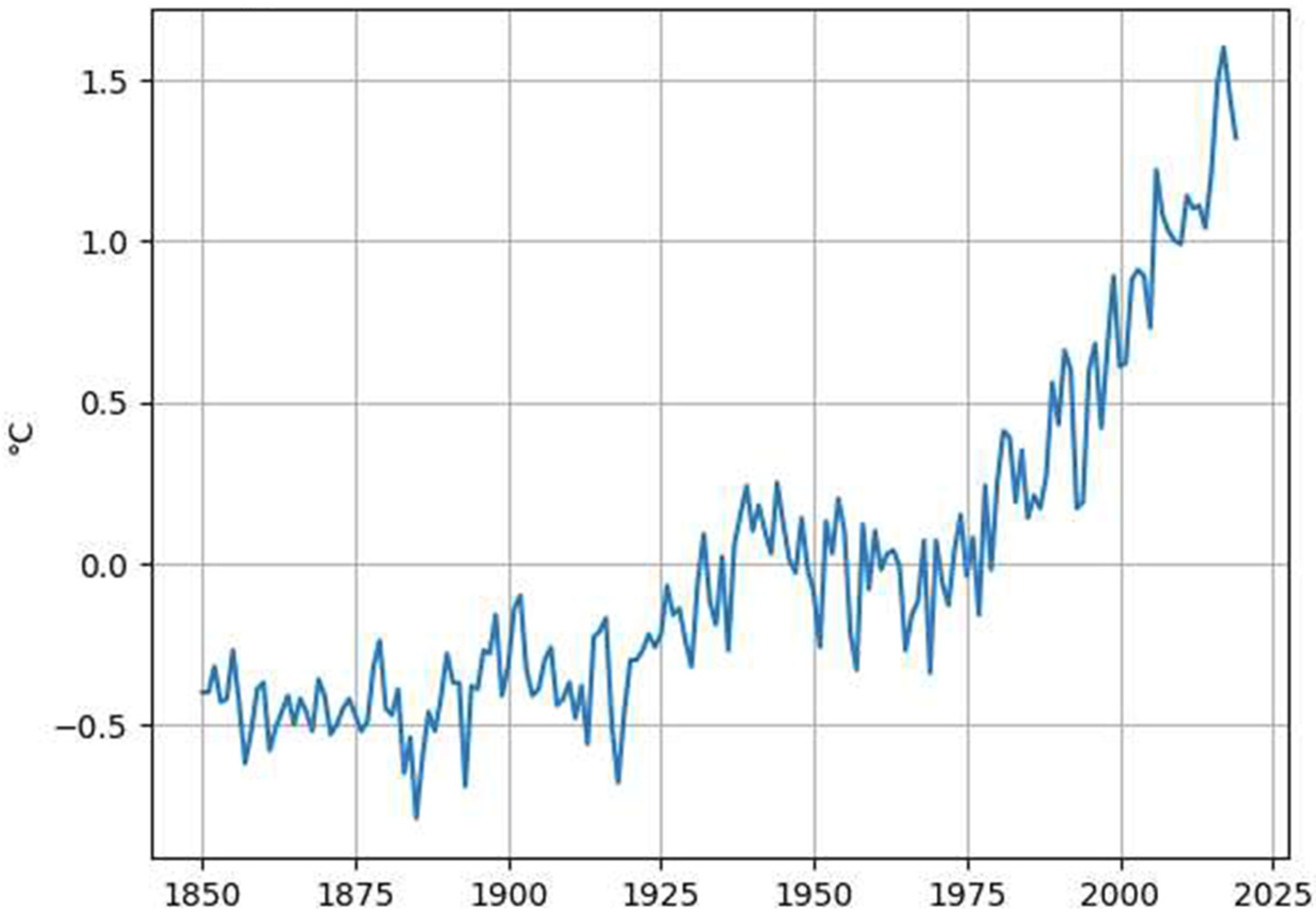
Figure 1 below illustrates the global temperature anomaly values for land areas from 1850 to 2019, as provided by NOAA.

${\mathrm{C}\mathrm{O}}_2$ emissions data were obtained from Our World in Data [24], a collaboration between the University of Oxford and the Global Change Data Lab. The dataset covers global emissions expressed in tons, with annual sampling over the period 1850–2019.

The Our World in Data dataset includes 257 geopolitical entities. The emissions data underwent a screening process to exclude states with negligible emissions (<1% overall). The screening process led to the exclusion of 115 countries. Once the essential 106 countries were identified, the next step involved subdividing them into subregions.

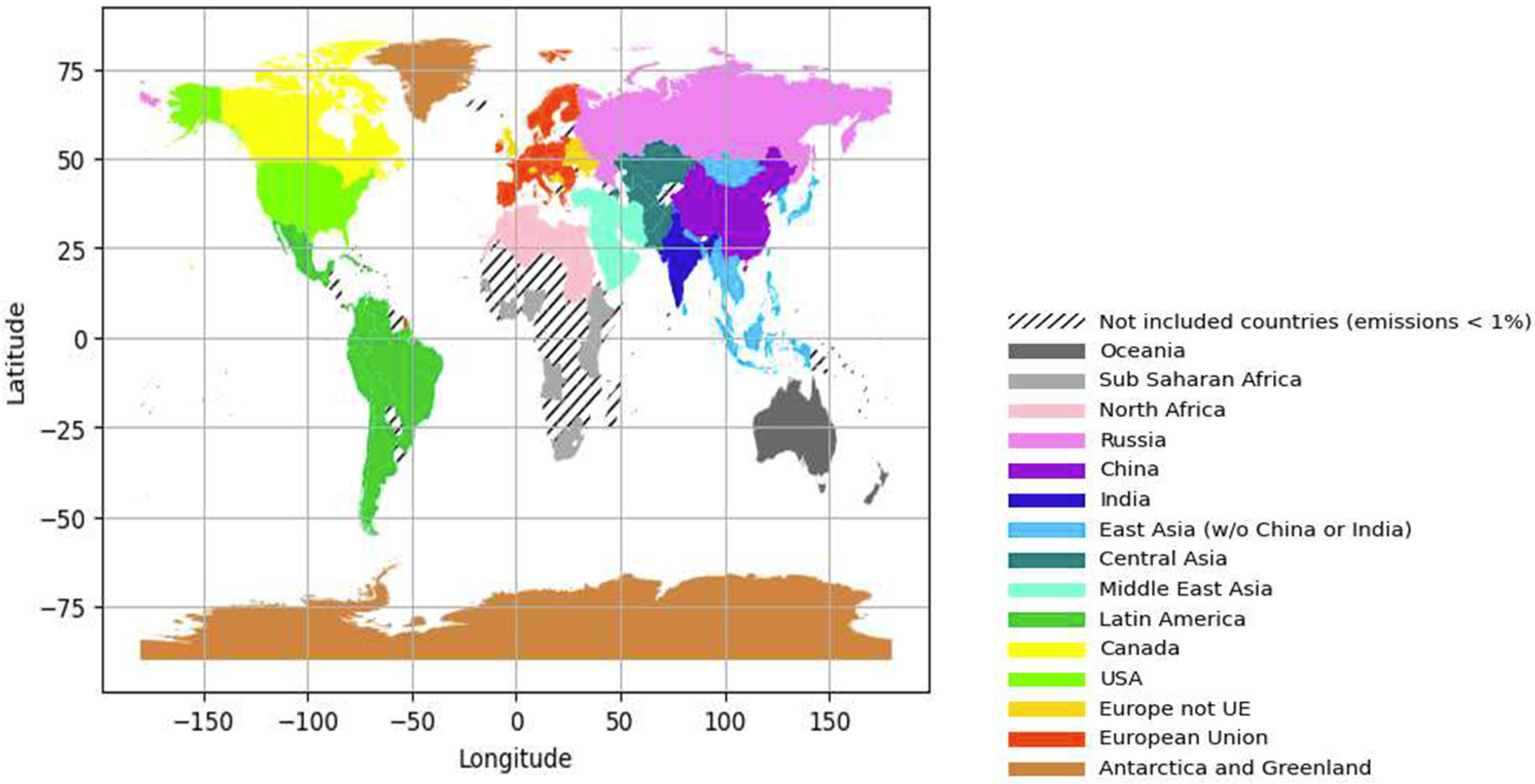
Since greenhouse gas emissions and temperature anomalies exhibit nonuniform spatial distribution, to accurately model this relationship in this work, the land areas were divided into 15 subregions, each comprising geographically or geopolitically similar countries (Figure 2).

For rice production (Figure 3), data published by FAOSTAT [25] were used. The dataset covers rice production statistics from 1960 to 2020 for Southeastern Asia, updated to 2020.

2.2. Case Study Overview: Southeast Asian Region Peculiarity

Despite the high degree of climate hazard in the Asian regions, subregional exposure and resilience vary. Geographical factors, economic progress, demographic dynamics, the importance of agriculture in the economy, urbanization rates, governance and institutions, and the strength of the national financial system all affect countries’ susceptibility to meteorological events and their ability to cope with severe natural disasters [12].

East Asia experiences temperature anomalies; however, the overall impact seems to be relatively moderate, mainly due to the advanced state of its economies [26].

Nevertheless, in this region, there are countries facing the greatest climate security challenges, and they are primarily located in Southeast Asia [27].

This study delineates Southeast Asia as comprising Bangladesh, the People’s Republic of Cambodia, Indonesia, the Lao People’s Democratic Republic, Myanmar, Nepal, the Philippines, Thailand, and Vietnam.

Southeast Asia has one of the fastest-growing economies. Nevertheless, this area is particularly susceptible to the impact of climate change and temperature variations, which harm agriculture, trade, healthcare, and infrastructure. The vulnerability of Southeast Asia stems from its long coastlines, which are densely populated, and the economic activity in these areas, which is characterized by a substantial reliance on agriculture for livelihoods, particularly among those living in poverty under USD 2 or USD 1 per day, and dependence on natural resources and forestry for development.

In recent decades, the region has experienced elevated temperatures and a higher frequency of extreme weather events, such as droughts, floods, and tropical cyclones, which pose a threat to economic activities, particularly agriculture. Agricultural output and food security are identified as primary areas of risk.

The agricultural sector in Southeast Asia currently employs around 300 million people (an increase since 1960) [17] and contributes 20–30% of the subregional gross domestic product (GDP) [24]. While there are variations in cereal production levels among countries, at least half of them derive more than 70% of their crop from cereals. The robust performance in cereal production and yield can be attributed to a longstanding policy pursued by Southeast Asian governments, which aims to achieve grain self-sufficiency for the purpose of ensuring food security.

Southeast Asia contributes 40% of global rice exports. Vietnam and Thailand are among the leading countries in this sector [28]. In 1961, rice accounted for 90.6% of the region’s cereal production and, still, this proportion remains almost unchanged. In 2020, rice accounted for 80.7% of the total cereal production, followed by maize (18.9%). Together, these provide 99.6% of the whole tonnage of cereal production [25]. Moreover, rice accounts for 50% of the calorie intake of the population in the area [29], and Asian rice (Oryza sativa L.) grown on farms is the main staple in the diet of many of the world’s most impoverished regions [30].

Adequate, affordable, and secure provision of rice is, therefore, essential for the region’s economic development and political stability.

This is why the methodology has been introduced and applied to assess the impact of temperature anomalies within the Southeastern Asian subregion, especially within the rice sector.

2.3. Data-Driven Model Calibration

The choice of a data-driven model framework for modeling the cause–effect link between $\mathrm{C}{\mathrm{O}}_2$ emissions and global temperature anomalies has been highly bounded by the scarcity of available data. Hence, a comparatively nimble model category has been implemented: the autoregressive model with exogenous input (ARX). An ARX model can link a phenomenon with its evolution in previous sampling instances (autoregressive part) with the presence of external factors (exogenous part).

Let $y\left(t\right)\in R$ and $u\left(t\right)\in R^{n_{ex}}$ be the values of the output variable and exogenous input for each time t, respectively.

Let $\mathsf{\Phi }{\left(t\right)}^T\in R^{n_a+n_b}$ be the vector of the measured values of the $n_a$ and $n_b$ terms of the autoregressive and exogenous part, respectively (note that u can be a vector), and $k$ be the delay between the exogenous input and the output.

$$\mathsf{\Phi }\left(t\right)=\left[y\left(t-1\right),\dots ,y\left(t-n_a\right),u\left(t-k\right),\dots ,u\left(t-n_b-k\right)\right]$$

(1)

Thus, the ARX model can be in general expressed as

$$y\left(t+1\right)=\mathsf{\Phi }\left(t\right)\cdot {\mathsf{\Theta }}^T,$$

(2)

where $\mathsf{\Theta }\in R^{na+nb}$ is the vector of the parameter to be estimated during the calibration phase. Usually, including this project, the estimation of the parameter vector $\mathsf{\Theta }$ is performed following the least-square method [31].

In the specific case, fifteen ARX models, one for each subregion, have been calibrated, considering the temperature anomaly (TA) of the individual subregion as the observed phenomenon (dependent variable). Exogenous factors (independent variables) include the global TAs, emissions from the same subregion, and the sum of emissions from all other subregions. Thus, in our case, $\mathsf{\Theta }={\left[{\mathsf{\Theta }}_{\mathrm{T}{\mathrm{A}}_{\mathrm{r}}},{\mathsf{\Theta }}_{\mathrm{T}{\mathrm{A}}_{\mathrm{g}}},{\mathsf{\Theta }}_{\mathrm{E}\mathrm{M}{\mathrm{I}}_{\mathrm{r}}},{\mathsf{\Theta }}_{\mathrm{E}\mathrm{M}{\mathrm{I}}_{\mathrm{o}}}\right]}^T$, where ${\mathsf{\Theta }}_{\mathrm{T}{\mathrm{A}}_{\mathrm{r}}},{\mathsf{\Theta }}_{\mathrm{T}{\mathrm{A}}_{\mathrm{g}}},{\mathsf{\Theta }}_{\mathrm{E}\mathrm{M}{\mathrm{I}}_{\mathrm{r}}},\mathrm{a}\mathrm{n}\mathrm{d} {\mathsf{\Theta }}_{\mathrm{E}\mathrm{M}{\mathrm{I}}_{\mathrm{o}}}$ are the parameter vectors for the autoregressive part (regional temperature anomaly, (${\mathsf{\Theta }}_{\mathrm{T}{\mathrm{A}}_{\mathrm{r}}}$), global temperature anomaly (${\mathsf{\Theta }}_{\mathrm{T}{\mathrm{A}}_{\mathrm{g}}}$), and regional (${\mathsf{\Theta }}_{\mathrm{E}\mathrm{M}{\mathrm{I}}_{\mathrm{r}}}$) and outside region emissions (${\mathsf{\Theta }}_{\mathrm{E}\mathrm{M}{\mathrm{I}}_{\mathrm{o}}}$)). The defined dataset (Section 2.1) includes yearly data from 1870 to 2019. The first 75% of the defined dataset (years 1870–1982) has been used for identification and the 25% for validation (years 1983–2019). Both calibration and validation have been performed considering the behavior of the system in the simulation phase, since a long forecasting horizon (tentatively from 2020 to 2100) must be addressed during the work. Once the family of the data-driven model was established, several tests were performed in order to select the orders of the different autoregressive and exogenous parts, defining the length of the different components of the vector parameter $\mathsf{\Theta }={\left[{\mathsf{\Theta }}_{\mathrm{T}{\mathrm{A}}_{\mathrm{r}}},{\mathsf{\Theta }}_{\mathrm{T}{\mathrm{A}}_{\mathrm{g}}},{\mathsf{\Theta }}_{\mathrm{E}\mathrm{M}{\mathrm{I}}_{\mathrm{r}}},{\mathsf{\Theta }}_{\mathrm{E}\mathrm{M}{\mathrm{I}}_{\mathrm{o}}}\right]}^T$ for each area. For each component $\left({\mathsf{\Theta }}_{\mathrm{T}{\mathrm{A}}_{\mathrm{r}}},{\mathsf{\Theta }}_{\mathrm{T}{\mathrm{A}}_{\mathrm{g}}},{\mathsf{\Theta }}_{\mathrm{E}\mathrm{M}{\mathrm{I}}_{\mathrm{r}}},{\mathsf{\Theta }}_{\mathrm{E}\mathrm{M}{\mathrm{I}}_{\mathrm{o}}}\right),$ a length ranging from 1 to 3 has been tested, resulting in $3^4=81$ configurations for each area, and the estimation has been performed for each of them.

Despite the nonlinearity and complexity of the involved phenomena, some physical constraints can be explicitly incorporated into the ARX model. This is based on the understanding that a decrease in emissions should correspond to a reduction in both global and regional temperature anomalies. This implies that the parameter values ${\mathsf{\theta }}_{\mathrm{E}\mathrm{M}{\mathrm{I}}_{\mathrm{r}}}$ and ${\mathsf{\theta }}_{\mathrm{E}\mathrm{M}{\mathrm{I}}_{\mathrm{o}}}$, related to subregion and other regions emissions, must be positive. These constraints lead to the need to solve an optimization problem to compute the parameter vector $\mathsf{\Theta }\mathrm{ }$:

$${\mathit{min}}_{\mathsf{\Theta }}‖y\left(t\right)-\overline{y}\left(t\right)‖$$

(3)

$$\mathrm{s}.t.$$

$$y\left(t+1\right)=\mathsf{\Phi }\left(t\right)\cdot \mathsf{\Theta }, t=1,\dots n$$

(4)

$$\mathsf{\Theta }={\left[{\mathsf{\Theta }}_{\mathrm{T}{\mathrm{A}}_{\mathrm{r}}},{\mathsf{\Theta }}_{\mathrm{T}{\mathrm{A}}_{\mathrm{g}}},{\mathsf{\Theta }}_{\mathrm{E}\mathrm{M}{\mathrm{I}}_{\mathrm{r}}},{\mathsf{\Theta }}_{\mathrm{E}\mathrm{M}{\mathrm{I}}_{\mathrm{o}}}\right]}^T$$

(5)

$${\mathsf{\Theta }}_{\mathrm{E}\mathrm{M}{\mathrm{I}}_{\mathrm{r}}}\mathrm{ }>0$$

(6)

$${\mathsf{\Theta }}_{\mathrm{E}\mathrm{M}{\mathrm{I}}_{\mathrm{o}}}\mathrm{ }>0,$$

(7)

where $\overline{y}\left(t\right)$ is the measured value of the output variable at time t, and n is the number of samples to be used in the calibration phase.

Even if a plethora of algorithms existed for the solution of such a problem [32], in this case, a genetic algorithm approach has been used [33].

2.4. Genetic Algorithm

The problem (3)–(7) is a nonlinear optimization problem due to the objective function (3) to be minimized and to the constraints (4) expressing the dynamic of the system across a simulation horizon of n samples. For this reason, in order to limit the possibility of obtaining a local minima as a solution, the genetic algorithm [34] approach has been adopted to compute the parameter vector $\mathsf{\Theta }$ for the independent variables of the ARX models.

Genetic algorithms are metaheuristic techniques that mimic the evolution of a group of individuals, drawing inspiration from natural selection and genetic mechanisms [34,35,36]. They generally consist of a finite population representing potential problem solutions, a fitness function gauging solution quality and identifying optimal individuals for reproduction, various operators that transition the current population to the next iteration, and a termination criterion determining when the algorithm should cease its operations.

The algorithm can be delineated into various phases:

• Population Initialization: initially, a set of individuals is created randomly. This population undergoes iterative evolution until an optimal solution is achieved.
• New Population Generation: this phase involves the evolution of the initial population through three key operations:

  ○

  Selection: like natural selection, this stage identifies the most promising candidates or solutions.

  ○

  Crossover: using the top candidates, hybrid solutions are produced, contributing to subsequent populations.

  ○

  Mutation: new individuals emerge through slight random alterations in the solutions of offspring.

• Termination Test: the process of generating the new population continues until one or more predefined stopping criteria are met. Some of the commonly used criteria include:

  ○

  Reaching a specified number of iterations.

  ○

  Reaching a set number of iterations without notable enhancement in the solution.

  ○

  Exceeding a predefined time threshold.

Table 1. Configuration of the genetic algorithm used for the calibration of the model.

Feature	Value
Population	100
Crossover Function	Scattered
Crossover Fraction	0.8
Mutation Function	Gaussian

presents the configuration used in the presented work.

3. Results and Discussion

The presented methodology has been applied to forecast the impact of temperature anomalies in East Asia in the period 2020–2100 and to evaluate the impact on rice production in this area. The first part of this case study will be devoted to the validation of the approach in terms of temperature anomalies, while in the second part, a deep discussion on the social and economic impacts of the forecasted variables will be presented.

3.1. ARX Model Validation

Table 2. Mean absolute error (MAE) and correlation coefficient for the identified ARX models for the validation dataset (the performances of East Asia, employed for this analysis, are highlighted).

Subregion	MAE	Correlation
Antarctica and Greenland	0.41	0.53
European Union	0.39	0.74
Europe outside EU	0.41	0.72
USA	0.30	0.77
Canada	0.53	0.67
South America	0.18	0.87
Middle East	0.32	0.80
Central Asia	0.50	0.69
East Asia	0.21	0.86
India	0.28	0.76
China	0.22	0.83
Russia	0.55	0.75
North Africa	0.23	0.84
Sub-Saharan Africa	0.16	0.87
Oceania	0.26	0.74

presents the validation results for the best model in each area, presented in terms of MAE (which is less affected by outliers with respect to the root mean squared error) and linear correlation coefficient. The performances are highly variable, thus highlighting the capability of the model to reproduce the trend for local temperature anomalies, as evidenced by the correlation coefficient reaching values higher than 0.8 for the Middle East, Africa, China, East Asia, and South America.

Due to the focus of this study, the East Asia model was used, which had the following structure:

$$\begin{gathered} T{A}_r\left(t\right)=0.2116T{A}_r\left(t-1\right)+0.00862T{A}_r\left(t-2\right)+0.0166T{A}_r\left(t-3\right)+03227T{A}_g\left(t-1\right)+0.0107EM{I}_r\left(t\right) \\ +0.0037EM{I}_o\left(t-1\right)\hspace{1em}\hspace{1em}\hspace{1em}\hspace{1em}\hspace{1em}\hspace{1em}\hspace{1em}\hspace{1em}\hspace{1em}\hspace{1em}\hspace{1em}\hspace{1em} \end{gathered}$$

(8)

By way of example, Equations (9) and (10) present the model for Europe (UE) and the USA, respectively:

$$\begin{gathered} T{A}_r\left(t\right)=0.2169T{A}_r\left(t-1\right)+0.113T{A}_r\left(t-2\right)+0.0822T{A}_r\left(t-3\right)+05708T{A}_g\left(t-1\right)-0.2801T{A}_g\left(t-1\right) \\ +0.0679EM{I}_r\left(t\right)+0.0039EM{I}_o\left(t-1\right)\hspace{1em}\hspace{1em}\hspace{1em}\hspace{1em}\hspace{1em}\hspace{1em} \end{gathered}$$

(9)

$$\begin{gathered} T{A}_r\left(t\right)=0.2816T{A}_r\left(t-1\right)+0.00761T{A}_r\left(t-2\right)+0.2867T{A}_r\left(t-3\right)+0.1179T{A}_g\left(t-1\right)+0.1179EM{I}_r\left(t\right) \\ +0.0884EM{I}_r\left(t-1\right)+0.5339EM{I}_o\left(t-1\right)\hspace{1em}\hspace{1em}\hspace{1em}\hspace{1em}\hspace{1em} \end{gathered}$$

(10)

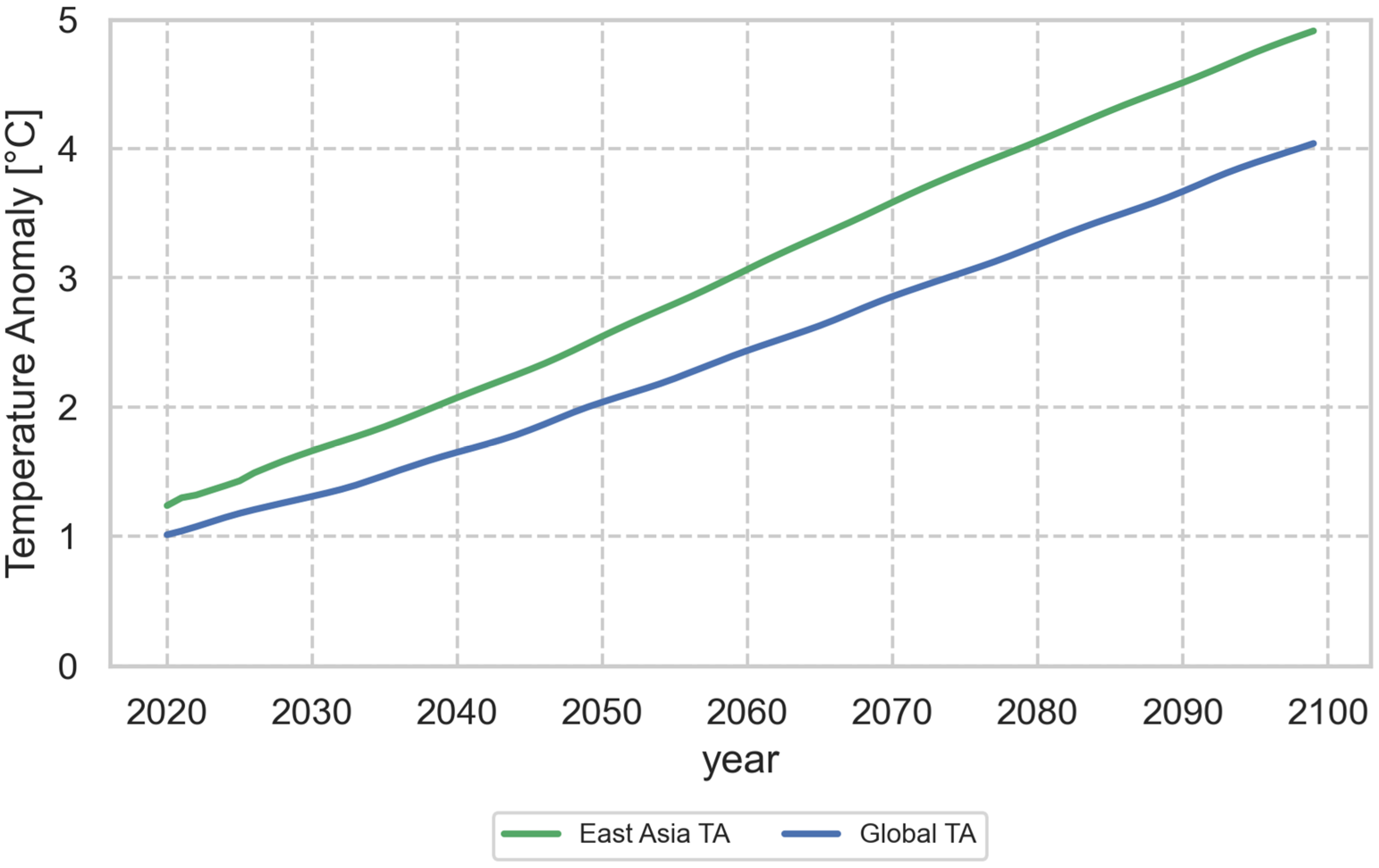
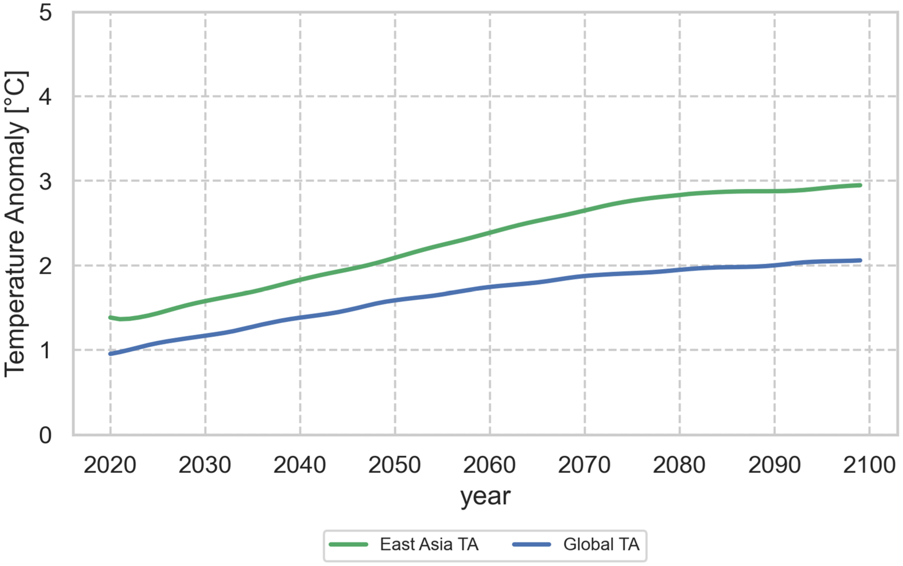
After validation, the model in Equation (8) was used to generate an estimation of the regional temperature anomaly for East Asia for the period 2020–2100, which was then compared to the global temperature anomaly data from the IPCC assessment report [12]. As shown by the time series, despite the influence of numerous nonlinear phenomena on temperature anomalies [12], the IPCC’s estimation for the RCP8.5 scenario from 2020 to 2100 appears nearly linear, as illustrated by the blue line in Figure 4. The model output reproduces a similar behavior for East Asia, even though its values are always higher than the global ones, suggesting a more significant climate change impact in this area. Nonetheless, in the RCP4.5 scenario (Figure 5), there is a decline in the temperature anomaly gradient after 2060. Similarly, in this case, the regional temperature anomaly generated by the model follows a similar pattern to the global temperature anomaly, although with values consistently higher. Even though the global temperature anomaly may exhibit nonlinear dynamics and behavior, the trends depicted in Figure 4 and Figure 5 align with findings in the literature [10,12].

In order to take into account the worst-case scenario, the analysis for the estimation of the impact of the temperature anomaly on rice production will be shown for the RCP8.5 scenario.

3.2. Impact of Temperature Anomaly on Rice Production

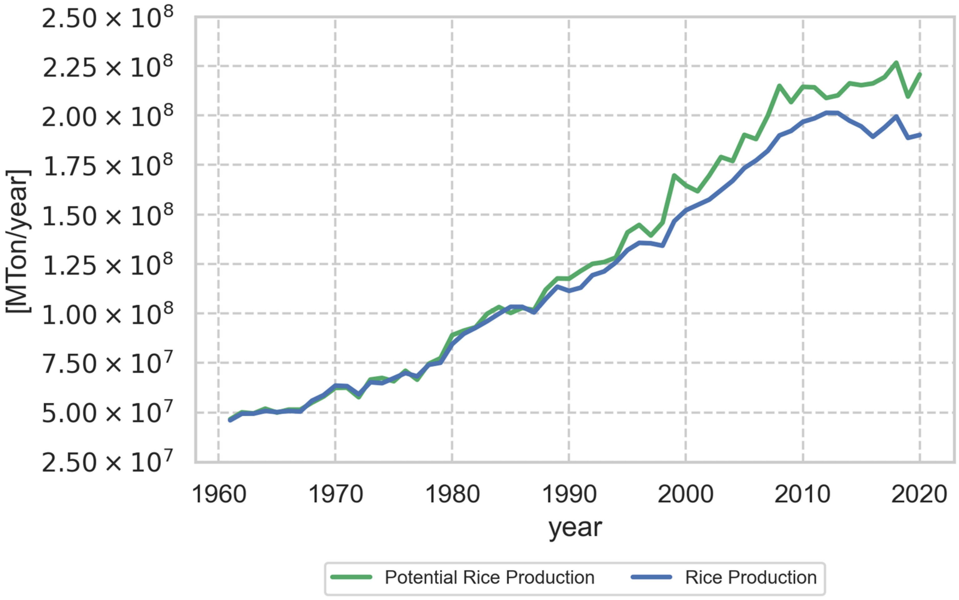
Rice production is influenced by several factors such as the availability of water, the quality of soil, the selection of rice varieties, the management of pests and diseases, the application of fertilizers, the control of weeds, the adoption of technology, changes in policies, socioeconomic issues, a careful management of land, and temperature anomalies [30]. Assessing the influence of temperature anomalies on rice production is, therefore, difficult since they serve as only one of the potential drivers influencing this complex process. Moreover, the available data sourced from FAOSTAT and spanning the period 1961–2020 [25], used for this study, are intrinsically affected by technological development, leading to a significant increase in production, even in recent decades, when the potential impact of temperature anomalies could have been notable. Therefore, the literature reports a 10% decrease in rice production for every 1 °C increase in temperature [26,37]. This information led the authors to approach the problem from a different perspective. Instead of evaluating the impact of other drivers, the methodology involved computing the potential production, i.e., the achievable production without the influence of temperature anomalies, over the period 2020–2100. Subsequently, the impact of the temperature anomaly was assessed using ARX models, which were evaluated and applied to the extrapolated data.

Let $P_r\left(t\right)$ be the FAOSTAT rice production in Southeast Asia during the period 1961–2020, and let $T{A}_r\left(t\right)$ be the temperature anomaly reported in that area by Berkeley Earth data. The potential rice production $P_r^o\left(t\right)$ could be computed as

$$P_r^o\left(t\right)=\frac{P_r\left(t\right)}{\left(1-T{A}_r\left(t\right)\times 0.1\right)}$$

(11)

Figure 6 presents the comparison between potential and actual rice production for the period 1961–2020 with the disparities between the two curves reaching a maximum peak of 2.5 × 10⁸ MTon/year in 2018.

The forecast of the potential rice production was then performed by means of an autoregressive model:

$$P_r^o\left(t\right)=0.9984P_r^o\left(t-1\right)+3157754,$$

(12)

which was identified using a least-square approach based on the 1961–2020 data. Despite the simplicity of this model with respect to the intricate dynamics of rice production (which should take into account both economical and innovation aspects), the simplified model in Equation (12) demonstrated strong performance for the specified period both in one-step ahead forecast and in simulation (

Table 3. Normalized mean absolute error (NMAE) and correlation coefficient for the potential rice production.

Subregion	1-Step Ahead	Simulation
NMAE	0.03	0.10
Correlation Coefficient	0.99	0.98

).

The chosen model and the prepared data were subsequently employed to predict the potential rice production trend for the period 2020–2100.

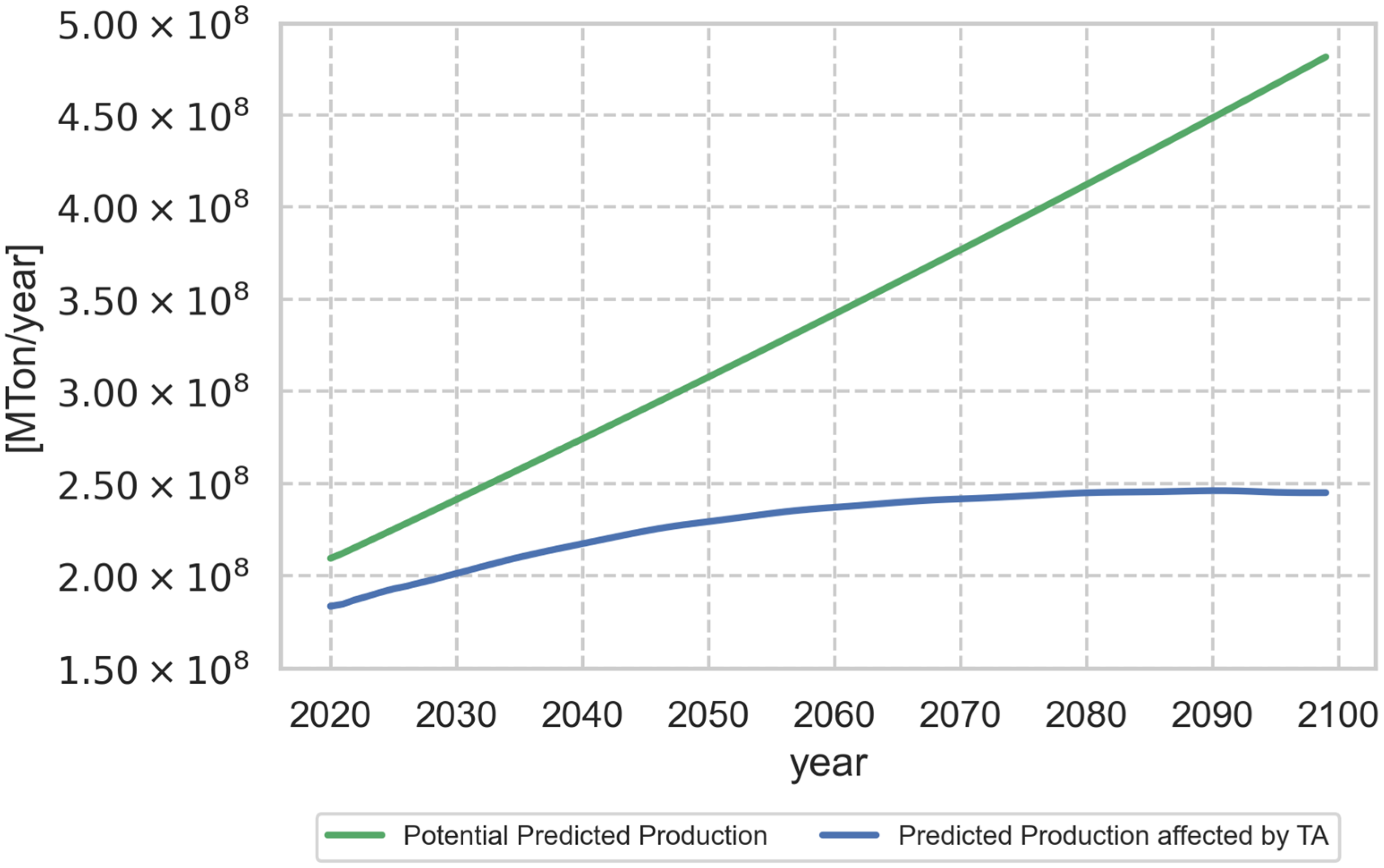
At this stage, it was possible to estimate the potential impact of temperature anomalies on rice production using (i) the temperature anomaly data obtained through the model described in the methodology section and referred to the East Asian subregion and (ii) the simple relation presented in [38,39], stating a 10% reduction in rice production for every 1 °C increase in temperature with respect to the potential production. This enabled the projection of the actual rice production that Southeast Asia might experience in the mentioned years. Figure 7 presents the comparison between the potential production and the predicted production considering the temperature anomaly effects for the period 2020–2100.

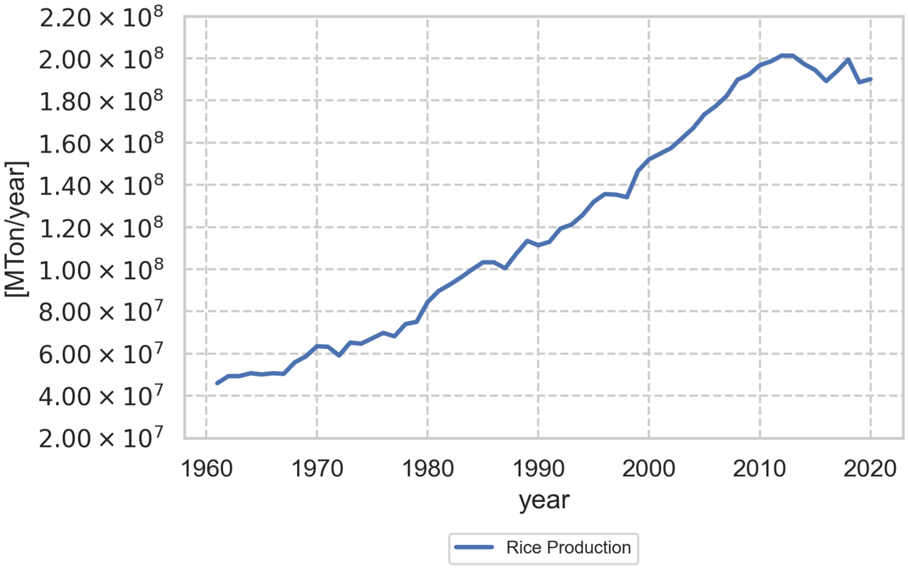
Since 1961 (Figure 6), it is evident that rice production has shown a nearly linear increase, primarily attributed to the “Green Revolution”, which was particularly successful in various countries, notably in parts of Latin America and Asia, including Southeast Asia. The Green Revolution in Southeast Asia encompassed a series of initiatives and innovations aimed at boosting agricultural productivity and food production. It primarily took place during the mid-20th century, starting in the 1960s. This transformative era was characterized by the development and adoption of high-yielding and more resilient crop varieties, particularly for rice and wheat. Moreover, it involved the adoption of modern farming techniques, including the use of fertilizers, pesticides, and herbicides, the expansion of irrigation systems, and the integration of advanced agricultural tools [40].

Furthermore, up until the 1980s, the temperature anomaly from the expected or average value was not significant and had limited impacts on rice production.

The temperature anomaly shows a worrying uptick, primarily attributed to anthropic activities, starting in the late 1980s. Indeed, a noticeable change in the presented model results is evident in the period 2020–2100 (Figure 5), when the temperature anomaly is expected to rise significantly. The data resulting from the model record a 240 Mton/year loss in rice production in 2100 compared to the potential rice production that could be achieved in that year and an overall loss of around 9000 Mton for the period 2020–2100 (115 Mton/year on average). The data align with the available literature, as numerous studies and publications support the findings, and report a decrease of 42–50% in grain yields by 2100 due to climate change and the worsening of soil quality [37,41]. Similarly, the report of the Asian Development Bank (2009) as well as FAO (2018) projected a potential decline of up to 50% in rice yield by 2100, attributed to climate change, when compared to 1990 levels [26,42].

The OECD-FAO Agricultural Outlook 2023–2032 predicts a 16% increase in crop production in South and Southeast Asia by 2032. This projection aligns with the $P_r^o$(t) in the previously presented model, although the model focuses solely on the Southeast Asia subregion, overlooking the South Asian subregion, as indicated in the OECD-FAO report, probably due to an underestimation of temperature anomaly effects in its projections.

3.3. Discussion

The estimated decrease of approximately 40–50% in rice harvests by 2100, as defined by the presented model, could have potentially devastating consequences in parts of the world where the harvest serves as a primary food source. A decline in supply is likely to impact domestic food security in numerous countries, potentially leading to malnutrition and health impairments, not only in Southeast Asia but also across the world. Indeed, food security becomes particularly severe in countries where agricultural systems are highly susceptible to changes in precipitation and temperature and where a significant proportion of households rely heavily on agriculture for income [43].

Despite significant economic growth that has lifted millions out of poverty, Southeast Asia remains one of the last strongholds of hunger. A substantial portion of the population in the region still grapples with food shortages, unable to meet their dietary energy requirements. In the region, there are 61 million people experiencing undernourishment, constituting approximately 9% of the population, with over 33 million facing severe food insecurity [44], and 18.8% of Southeast Asians continue to live below the poverty line of USD 1.25 a day [26].

In rural areas, farmers commonly set aside a portion of their cereal harvest for personal consumption. Likewise, landless laborers engaged in fieldwork frequently receive part of their compensation in the form of grains [45]. The anticipated decrease in rice production thus presents a substantial threat to food security for local farmers and their families.

Furthermore, certain Southeast Asian countries exhibit a notably high percentage of women engaged in agriculture, exceeding 60% in Laos, for instance [27]. Consequently, a decrease in crop production could potentially affect the social and economic well-being of these women.

In addition to the broad economic impact of temperature anomalies on the region, political and social dimensions play a crucial role in evaluating climate risks. The escalation of food and water insecurity, along with soil loss, may heighten the potential for social instability and conflict. Tensions and conflicts between states could intensify in areas crucial for water access. For example, if water volumes decrease significantly, China, controlling the upstream flows of major rivers in the region (e.g., Mekong and Ganges), is likely to prioritize internal use, particularly given the recurring periods of drought predicted in the country.

Mass migrations, resulting from the deepening impacts of climate change within and between states, will also contribute to the risks of tension and conflict. According to the Intergovernmental Panel on Climate Change (IPCC), natural disasters in Southeast Asia and East Asia in 2019 displaced over 10 million people, nearly 30% of global displacements, and it is anticipated that this number will rise in the long term [1].

4. Conclusions

Given the crucial importance of rice in emerging Asian countries as a key dietary component and a valuable export, it is essential to boost its production to keep pace with increasing demand due to population growth and to fortify its resilience against temperature anomalies.

Countries in Southeast Asia have gleaned insights from previous occurrences and dedicated resources toward readiness, mitigation, and minimizing risks. They have formulated national and local strategies focused on informed risk management and well-coordinated systems, along with implementing early warning mechanisms, irrigation initiatives, and disaster readiness plans. As an example, to tackle projected drought, Thailand has developed a comprehensive national water management plan, while Malaysia has established a ‘war room’ to monitor its reservoirs.

Yet, there is a substantial concern that numerous mitigation strategies are primarily reactive, addressing the structural repercussions of climate change after they have occurred. Comparable to other areas, the rate of adaptation is not matching the accelerating challenges posed by climate change. This calls for an immediate overhaul of energy systems, land management, ecosystems, and urban development—a fundamental structural transformation—rather than relying solely on a sequence of adaptation measures. This scenario encompasses various factors, such as physical space, income and development levels, institutional quality, political instability, and often a lack of awareness of risks. Simultaneously, the more significant the delay in undertaking substantial investments and courageous systemic changes in Southeast Asia, the more severe the impact of climate risks on future country risks will become.

Additional measures and varied strategic approaches could be employed to fortify the resilience of rice agricultural systems against diverse climatic shocks. These may involve advocating water-conservation technologies and improving irrigation systems to mitigate the adverse effects of droughts, thereby enhancing food security. Strengthening breeding initiatives aimed at developing climate-adaptive rice varieties capable of enduring environmental stresses, ensuring the availability of high-quality seeds, educating consumers about diversifying staple foods with drought-resistant crops, augmenting rice reserves, supporting open rice trade, and fostering regional collaboration are effective actions and advancements in rice research.

From a modeling standpoint, this research must be recognized as preliminary within a larger research framework whose main goal is to tackle the primary constraints presented in this study, notably the lack of data for regional temperature anomaly model calibration.

To make significant progress, a pivotal step forward involves the incorporation of a more extensive dataset, especially monthly data. This aims to bolster the reliability of both the estimation and validation processes, which is essential for enhancing the comprehension of regional temperature anomalies and, consequently, improving the accuracy of the modeling outcomes. The increased size of the dataset would lead to a more advanced examination of historical trends and a more thorough evaluation of the various factors contributing to regional temperature anomalies. Although the developed system is simple and requires few computational resources, it has significant potential for further extension beyond its current degree of sophistication.

Finally, future plans include incorporating this approach into a model predictive control (MPC) framework. This integration allows for a more dynamic and responsive decision-making paradigm. This transition would represent a shift from basic data analysis to a proactive strategy, considering both global and regional impacts in real time to improve information provision and decision-making processes.

References

- Intergovernmental Panel on Climate Change Climate Change 2021—The Physical Science Basis, 1st ed.; Working Group I Contribution to the Sixth Assessment Report of the Intergovernmental Panel on Climate Change; Cambridge University Press: Cambridge, UK, 2023; ISBN 978-1-00-915789-6.
- Sathaye, J.; Najam, A.; Cocklin, C.; Heller, T.; Lecocq, F.; Llanes-Regueiro, J.; Pan, J.; Petschel-Held, G.; Rayner, S.; Robinson, J.; et al. Sustainable Development and Mitigation. In Climate Change 2007: Mitigation; Contribution of Working Group III to the Fourth Assessment Report of the Intergovernmental Panel on Climate Change; Metz, B., Davidson, O.R., Bosch, P.R., Dave, R., Meyer, L.A., Eds.; Cambridge University Press: Cambridge, UK, 2007. [Google Scholar]
- United Nations. Environment Programme Emissions Gap Report 2023: Broken Record—Temperatures Hit New Highs, yet World Fails to Cut Emissions (Again); United Nations Environment Programme: Nairobi, Kenya, 2023; ISBN 978-92-807-4098-1. [Google Scholar]
- World Meteorological Organization (WMO); United Nations Environment Programme (UNEP); Intergovernmental Panel on Climate Change (IPCC); Global Carbon Project (GCP); UK Met Office; United Nations Office for Disaster Risk Reduction (UNDRR). United in Science 2022—A Multi-Organization High-Level Compilation of the Most Recent Science Related to Climate Change, Impacts and Responses; WMO: Geneva, Switzerland, 2022.
- United Nations. Long-Term Low-Emission Development Strategies Synthesis Report. In Proceedings of the Conference of the Parties Serving as the Meeting of the Parties to the Paris Agreement, Fourth Session, Sharm el-Sheikh, Egypt, 6–20 November 2022. [Google Scholar]
- Boyd, S.; Roach, R. Feeling the Heat: Why Government Must Act to Tackle the Impact of Climate Change on Global Water Supplies and Avert Mass Movement of Climate Change Refugees; Tearfund: London, UK, 2006. [Google Scholar]
- Burke, E.J.; Brown, S.J.; Christidis, N. Modeling the Recent Evolution of Global Drought and Projections for the Twenty-First Century with the Hadley Centre Climate Model. J. Hydrometeorol. 2006, 7, 1113–1125. [Google Scholar] [CrossRef]
- Intergovernmental Panel on Climate Change Climate Change and Land. IPCC Special Report on Climate Change, Desertification, Land Degradation, Sustainable Land Management, Food Security, and Greenhouse Gas Fluxes in Terrestrial Ecosystems, 1st ed.; Cambridge University Press: Cambridge, UK, 2022; ISBN 978-1-00-915798-8. [Google Scholar]
- Carnevale, C.; Sangiorgi, L. A Receding Horizon Approach for Climate Change Control. In Proceedings of the 2023 9th International Conference on Control, Decision and Information Technologies (CoDIT), Rome, Italy, 3 July 2023; pp. 257–262. [Google Scholar]
- Eyring, V.; Bony, S.; Meehl, G.A.; Senior, C.A.; Stevens, B.; Stouffer, R.J.; Taylor, K.E. Overview of the Coupled Model Intercomparison Project Phase 6 (CMIP6) Experimental Design and Organization. Geosci. Model Dev. 2016, 9, 1937–1958. [Google Scholar] [CrossRef]
- Our World in Data. CO2 Emissions (Form the University of Oxford and GCDL). Available online: https://ourworldindata.org/co2-emissions (accessed on 7 September 2023).
- Intergovernmental Panel on Climate Change (IPCC). Climate Change 2022—Impacts, Adaptation and Vulnerability, 1st ed.; Working Group II Contribution to the Sixth Assessment Report of the Intergovernmental Panel on Climate Change; Cambridge University Press: Cambridge, UK, 2023; ISBN 978-1-00-932584-4. [Google Scholar]
- Easterling, W.; Aggarwal, P.; Batima, P.; Brander, K.; Erda, L.; Howden, M.; Kirilenko, A.; Morton, J.; Soussana, J.-F.; Schmidhuber, S.; et al. Food, Fiber and Forest Products. In Climate Change 2007: Impacts, Adaptation and Vulnerability; Contribution of Working Group II to the Fourth Assessment Report of the Intergovernmental Panel on Climate Change; Cambridge University Press: Cambridge, UK, 2007. [Google Scholar]
- Lobell, D.B.; Gourdji, S.M. The Influence of Climate Change on Global Crop Productivity. Plant Physiol. 2012, 160, 1686–1697. [Google Scholar] [CrossRef] [PubMed]
- Kurukulasuriya, P.; Rosenthal, S. Climate Change and Agriculture a Review of Impacts and Adaptations; Climate Change Series Paper; World Bank: Washington, DC, USA, 2003. [Google Scholar]
- Field, C.B.; Barros, V.R. Climate Change 2014: Impacts, Adaptation, and Vulnerability; Working Group II Contribution to the Fifth Assessment Report of the Intergovernmental Panel on Climate Change; Cambridge University Press: New York, NY, USA, 2014; ISBN 978-1-107-64165-5. [Google Scholar]
- FAO. FAO Strategy on Climate Change; FAO: Roma, Italy, 2017. [Google Scholar]
- National Intelligence Council Southeast Asia and Pacific Islands: The Impact of Climate Change to 2030; National Intelligence Council: Washington, DC, USA, 2009.
- Bhandari, S.R. Asia’s Heatwaves 30 Times More Likely Due to Climate Change, Scientists Say. Radio Free Asia. 2023. Available online: https://www.rfa.org/english/news/environment/asia-heatwave-05182023020840.html (accessed on 28 January 2024).
- AFSIS. Rice Growing Outlook Report; AFSIS: New York, NY, USA, 2020. [Google Scholar]
- AFSIS. Rice Growing Outlook Report; AFSIS: New York, NY, USA, 2021. [Google Scholar]
- Copernicus Climate Change Service. Temperature and Precipitation Gridded Data for Global and Regional Domains Derived from In-Situ and Satellite Observations. Available online: https://cds.climate.copernicus.eu/doi/10.24381/cds.11dedf0c (accessed on 14 September 2023).
- Vose, R.S.; Arndt, D.; Banzon, V.F.; Easterling, D.R.; Gleason, B.; Huang, B.; Kearns, E.; Lawrimore, J.H.; Menne, M.J.; Peterson, T.C.; et al. NOAA’s Merged Land–Ocean Surface Temperature Analysis. Bull. Am. Meteorol. Soc. 2012, 93, 1677–1685. [Google Scholar] [CrossRef]
- Our World in Data. Agricultural Production. Available online: https://ourworldindata.org/agricultural-production (accessed on 11 October 2023).
- FAO. Crops and Livestock Products; FAO: Rome, Italy, 2021. [Google Scholar]
- Asian Develoopment Bank. The Economics of Climate Change in Southeast Asia: A Regional Review; Asian Develoopment Bank: Sydney, Australia, 2009; ISBN 978-971-561-787-1. [Google Scholar]
- Our World in Data. Employment in Agriculture. Available online: https://ourworldindata.org/employment-in-agriculture (accessed on 28 January 2024).
- Yuan, S.; Stuart, A.M.; Laborte, A.G.; Rattalino Edreira, J.I.; Dobermann, A.; Kien, L.V.N.; Thúy, L.T.; Paothong, K.; Traesang, P.; Tint, K.M.; et al. Southeast Asia Must Narrow down the Yield Gap to Continue to Be a Major Rice Bowl. Nat. Food 2022, 3, 217–226. [Google Scholar] [CrossRef] [PubMed]
- Sun, C.; Zhang, H.; Xu, L.; Ge, J.; Jiang, J.; Zuo, L.; Wang, C. Twenty-Meter Annual Paddy Rice Area Map for Mainland Southeast Asia Using Sentinel-1 Synthetic-Aperture-Radar Data. Earth Syst. Sci. Data 2023, 15, 1501–1520. [Google Scholar] [CrossRef]
- Dawe, D.; Pandey, S.; Nelson, A. Emerging Trends and Spatial Patterns of Rice Production. In Rice in the Global Economy: Strategic Research and Policy Issues for Food Security; Pandey, S., Byerlee, D., Dawe, D., Dovermann, A., Mohanty, S., Rozelle, S., Hardy, B., Eds.; International Rice Research Institute: Los Baños, Philippines, 2010; pp. 15–35. ISBN 978-971-22-0258-2. [Google Scholar]
- Ljung, L. System Identification: Theory for the User, 2nd ed.; Prentice Hall Information and System Sciences Series; Prentice Hall PTR: Upper Saddle River, NJ, USA, 1999; ISBN 978-0-13-656695-3. [Google Scholar]
- Ehrgott, M. Multicriteria Optimization; Springer Science & Business Media: Berlin/Heidelberg, Germany, 2005; Volume 491. [Google Scholar]
- Gallagher, K.; Sambridge, M.; Drijkoningen, G. Genetic Algorithms: An Evolution from Monte Carlo Methods for Strongly Non-Linear Geophysical Optimization Problems. Geophys. Res. Lett. 1991, 18, 2177–2180. [Google Scholar] [CrossRef]
- Wang, H.; Lang, X.; Mao, W. Voyage Optimization Combining Genetic Algorithm and Dynamic Programming for Fuel/Emissions Reduction. Transp. Res. Part D 2021, 90, 102670. [Google Scholar] [CrossRef]
- Beasley, J.E.; Chu, P.C. A Genetic Algorithm for the Set Covering Problem. Eur. J. Oper. Res. 1996, 94, 392–404. [Google Scholar] [CrossRef]
- Li, J.; Zhang, H.; Luo, Y.; Deng, X.; Grieneisen, M.L.; Yang, F. Stepwise Genetic Algorithm for Adaptive Management: Application to Air Quality Monitoring Network Optimization. Atmos. Environ. 2019, 215, 116894. [Google Scholar] [CrossRef]
- Peng, S.; Huang, J.; Sheehy, J.E.; Laza, R.C.; Visperas, R.M.; Zhong, X.; Centeno, G.S.; Khush, G.S.; Cassman, K.G. Rice Yields Decline with Higher Night Temperature from Global Warming. Proc. Natl. Acad. Sci. USA 2004, 101, 9971–9975. [Google Scholar] [CrossRef] [PubMed]
- Amnuaylojaroen, T.; Parasin, N. The Future Extreme Temperature under RCP8.5 Reduces the Yields of Major Crops in Northern Peninsular of Southeast Asia. Sci. World J. 2022, 2022, 1410849. [Google Scholar] [CrossRef] [PubMed]
- Matthews, R.B.; Kropff, M.J.; Horie, T.; Bachelet, D. Simulating the Impact of Climate Change on Rice Production in Asia and Evaluating Options for Adaptation. Agric. Syst. 1997, 54, 399–425. [Google Scholar] [CrossRef]
- Farmer, B.H. The “Green Revolution” in South Asia. Geography 1981, 66, 202–207. [Google Scholar]
- Muehe, E.M.; Wang, T.; Kerl, C.F.; Planer-Friedrich, B.; Fendorf, S. Rice Production Threatened by Coupled Stresses of Climate and Soil Arsenic. Nat. Commun. 2019, 10, 4985. [Google Scholar] [CrossRef] [PubMed]
- Sekhar, C.S.C. Climate Change and Rice Economy in Asia: Implications for Trade Policy; FAO: Roma, Italy, 2018. [Google Scholar]
- Ripple, W.J.; Wolf, C.; Newsome, T.M.; Barnard, P.; Moomaw, W.R. World Scientists’ Warning of a Climate Emergency. BioScience 2019, 70, biz088. [Google Scholar] [CrossRef]
- FAO; IFAD; UNICEF; WFP; WHO. The State of Food Security and Nutrition in the World 2023; FAO: Rome, Italy, 2023; ISBN 978-92-5-137226-5. [Google Scholar]
- Pingali, P. Agricultural Policy and Nutrition Outcomes—Getting beyond the Preoccupation with Staple Grains. Food Secur. 2015, 7, 583–591. [Google Scholar] [CrossRef]
Figure 1.
Global temperature anomaly values for land areas from 1850 to 2019 as provided by NOAA [23].
Figure 2.
Regional segmentation for the domain under study.
Figure 3.
Rice production [Mton/year] for the period 1961–2020 [25].
Figure 4.
Comparison between global [12] and regional temperature anomaly estimated for RCP8.5 by model for the period 2020–2100 [°C].
Figure 5.
Comparison between global [12] and regional temperature anomaly estimated for RCP4.5 by model for the period 2020–2100 [°C].
Figure 6.
Potential production (, green) and production affected by temperature anomaly (, blue) [25] for the period 1961–2020 [MTon/year].
Figure 7.
Potential production trend (, green) and production affected by temperature anomaly (, blue) 2020–2100 [MTon/year].