Predictive Analytics of Air Temperature in Alaskan Permafrost Terrain Leveraging Two-Level Signal Decomposition and Deep Learning

Abstract

Local weather forecasts in the Arctic outside of settlements are challenging due to the dearth of ground-level observation stations and high computational costs. During winter, these forecasts are critical to help prepare for potentially hazardous weather conditions, while in spring, these forecasts may be used to determine flood risk during annual snow melt. To this end, a hybrid VMD-WT-InceptionTime model is proposed for multi-horizon multivariate forecasting of remote-region temperatures in Alaska over short-term horizons (the next seven days). First, the Spearman correlation coefficient is employed to analyze the relationship between each input variable and the forecast target temperature. The most output-correlated input sequences are decomposed using variational mode decomposition (VMD) and, ultimately, wavelet transform (WT) to extract time-frequency patterns intrinsic in the raw inputs. The resulting sequences are fed into a deep InceptionTime model for short-term forecasting. This hybrid technique has been developed and evaluated using 35+ years of data from three locations in Alaska. Different experiments and performance benchmarks are conducted using deep learning models (e.g., Time Series Transformers, LSTM, MiniRocket), and statistical and conventional machine learning baselines (e.g., GBDT, SVR, ARIMA). All forecasting performances are assessed using four metrics: the root mean squared error, the mean absolute percentage error, the coefficient of determination, and the mean directional accuracy. Superior forecasting performance is achieved consistently using the proposed hybrid technique.

1. Introduction

Infrastructure and natural environments in polar areas underlain by permafrost at temperatures near 0 ${}^{°}\mathrm{C}$ are vulnerable to short- and long-term disturbances. Specifically, the climate-driven changes to the permafrost landscape of the US Arctic provide numerous terrain-related challenges [1]. For example, the thawing of the permanently frozen ice-bearing regolith can result in the rapid collapse of the soil surface, degradation of roads and railroad embankments, and turn previously solid ground into muddy, waterlogged terrain, unnavigable by vehicle or on foot in summer months.

Permanently frozen ground, or permafrost, covers extended regions of the Earth. In a vertical section, the permafrost, by definition, begins at the bottom of the seasonally freezing and thawing surficial layer, called the active layer, and extends further down. The total thickness of permafrost varies from site to site, from a fraction of a meter in southern parts of the Arctic to over 1000 m in Siberia. For periods of years to tens of years, the permafrost temperatures typically change minimally unless disrupted by surficial changes in forest fires, snow depth, or climate. Most of the annual infrastructure damage and human-perceived problems in permafrost areas, come from the phase change of the water to ice and ice to water within the active layer and/or the melting of the permafrost.

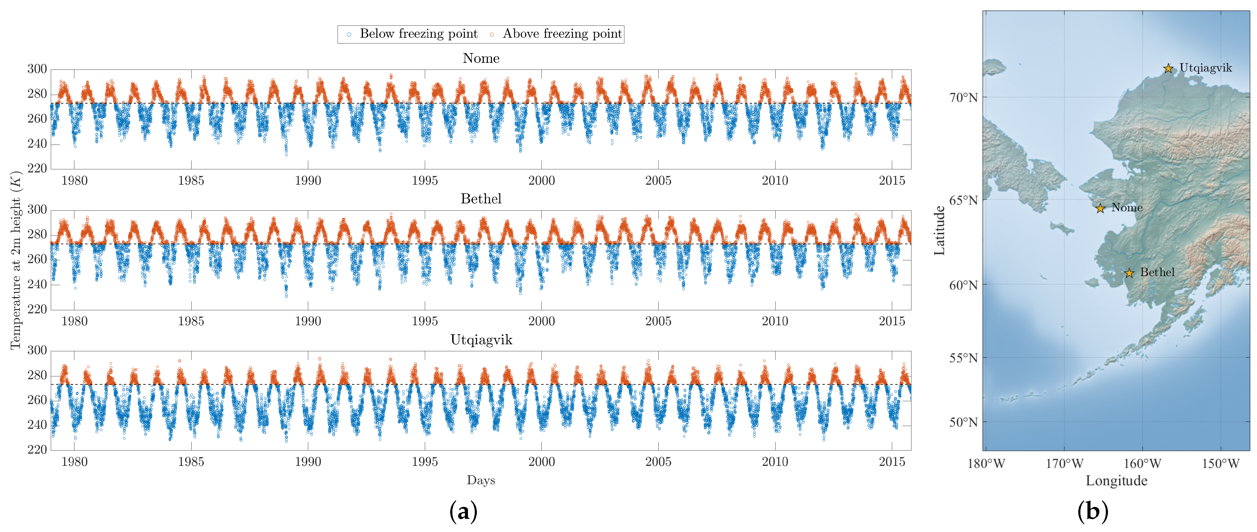
Various drivers are behind thermal changes in permafrost. Long-term (e.g., years and tens of years) changes in boundary conditions can lead to changes in the permafrost thermal regime. For short-term (e.g., weekly, monthly, annual) variations of permafrost and especially the active layer thermal regime, the weather is the most important driver. Therefore, accurate measurement of air temperature can provide insights into thermal effects occurring underground. Such monitoring is especially important in regions of the Arctic where the permafrost temperatures are already close to 0 ${}^{°}\mathrm{C}$.

However, in Alaska and elsewhere in the Arctic, accurate local weather forecasts are often available only for cities and larger settlements. In addition, the temperature in these regions can be volatile and fluctuating, rapidly plunging from near 0 ${}^{°}\mathrm{C}$ to −30 °C or lower. Moreover, traditional weather forecasting in remote Arctic regions is challenging due to the sparse network of ground stations providing real-time observations. The operational climate models that are regularly used for forecasting are physics-based fluid dynamics models aided by historical statistics, and they are guided by observed real-time near surface and atmospheric observations. Due to the lack of surface observations, however, the models are forced to interpolate across vast spaces of terrain. Therefore the forecast at any given point located far from the ground stations is, at best, an interpolated estimate.

Various methods have been proposed in the literature to forecast air temperature. Two main categories can be distinguished: physical models and statistical models. The first category includes numerical weather prediction models [2,3]. Although such models rely on physics-based modeling, they constitute large-scale models as they have a relatively large resolution (i.e., their grid spacing is greater than the local scale), require high computational costs, and might not be as accurate under certain meteorological and terrain conditions. Several studies have shown that incorporating post-processing techniques with these models can reduce their forecasting errors [4,5]. Diverse correction methods from statistical models, such as model output statistics [6] and local dynamical analog [7], to machine learning models, such as support vector regressions (SVRs), convolutional neural networks (CNNs), and gated recurrent units (GRU) [5,8], have all been proposed to improve the performance of numerical weather models. Nevertheless, these techniques generally require a large computational capacity as they rely on massive numerical simulations and post-processing approaches to achieve finer-scale end-user forecasts [9].

In the second category, data-driven techniques have been leveraged in the literature to achieve end-to-end forecasting in primarily non-arctic environments. Such methods include simple statistical time series models, such as the auto-regressive integrated moving average (ARIMA) and its variants [10,11], and conventional machine learning techniques, such as SVR, Random Forest (RF), and shallow neural networks [12,13,14]. For instance, the authors of [10] developed a seasonal ARIMA model through the use of the Box and Jenkins method to predict long-term air temperature in the city of Tetuán, Morocco. Model learning was conducted using the monthly average air temperature data spanning from 1980 to 2022. In [15], the authors investigated the effect of a combination of weather variables using a shallow neural network to predict the maximum temperature during the winter season of Tehran, Iran. This study employed monthly weather data spanning from 1951 to 2010. In [16], the authors investigated conventional machine learning techniques for short-term single-horizon air temperature forecasts in Crary City in North Dakota, USA. Specifically, SVR, Regression Tree, Quantile Regression Tree, ARIMA, RF, and Gradient Boosting Regression, were trained and tested on a chronologically split time series temperature dataset of daily and weekly averages spanning from 2000 to 2021. Model performance was assessed using the root mean square error (RMSE), the correlation coefficient, Thiels’ U-statistics, and the mean absolute error (MAE), with RF providing the highest performance. These shallow machine learning techniques, however, have demonstrated limited performance.

In recent years, deep learning techniques have attracted increased attention in a wide range of fields and within this research area as well. Their success can be attributed to the increase in computational power, the availability of large datasets, and the rapid development of newer and more sophisticated architectures. For instance, the authors of [17], investigated deep learning models for short-term single- and multi-horizon forecasting using data from JFK Airport, New York. Particularly, a long short-term memory (LSTM) model, a combination of CNN and LSTM, as well as multi-layer perceptron, were developed for one- to 10-day ahead forecasting. Model learning was conducted using the past seven days of wind speed, precipitation, snow depth, and mean, maximum, and minimum temperature data spanning from 2009 to 2019. Model performance was assessed using RMSE and the mean absolute percentage error (MAPE). The results highlighted the superiority of the CNN-LSTM model. In [18], the authors addressed long-term multi-horizon air temperature forecasting using an attention-based network with an encoder–decoder architecture. This model learned the average daily temperature time series of five cities from Spain, India, New Zealand, and Switzerland spanning over 25 years. Model performance was assessed using several metrics, including RMSE, MAPE, and the coefficient of determination ($R^2$). The proposed model provided higher performance than different statistical and machine learning models. Despite the improved performances achieved by these deep data-driven models, forecasting air temperature remains a challenging undertaking due to its complex and fluctuating processes.

There is a combination of regularity and stochasticity that governs the temperature of the air, which makes air temperature time series generally highly fluctuating and non-stationary. Yet, the current literature does not consider addressing these inherent issues within data-driven techniques. Instead, they rely primarily on the ability of the machine learning model to accurately predict future patterns in the temperature. In addition, numerous studies evaluate their proposed techniques using temperature data acquired from a single location, overlooking the impact that different geographical and climatic conditions may have on its accuracy.

As a means of addressing these issues, this paper aims to build better operational capability to forecast air temperature at the local scale (1 km) based on limited on-site observations. To enhance the predictions’ accuracy, data-driven techniques can be employed. Specifically, a combination of data processing techniques and advances in deep learning techniques can bypass inherent issues with the input data, reveal their hidden patterns, and improve forecasting accuracy. Moreover, while the proposed technique relies on past air temperature and specific humidity data due to their availability and their established roles as primary indicators of atmospheric dynamics, it offers a pragmatic and computationally economic approach to forecasting the air temperature in areas with sparse observational data.

More specifically, this work makes the following main contributions:

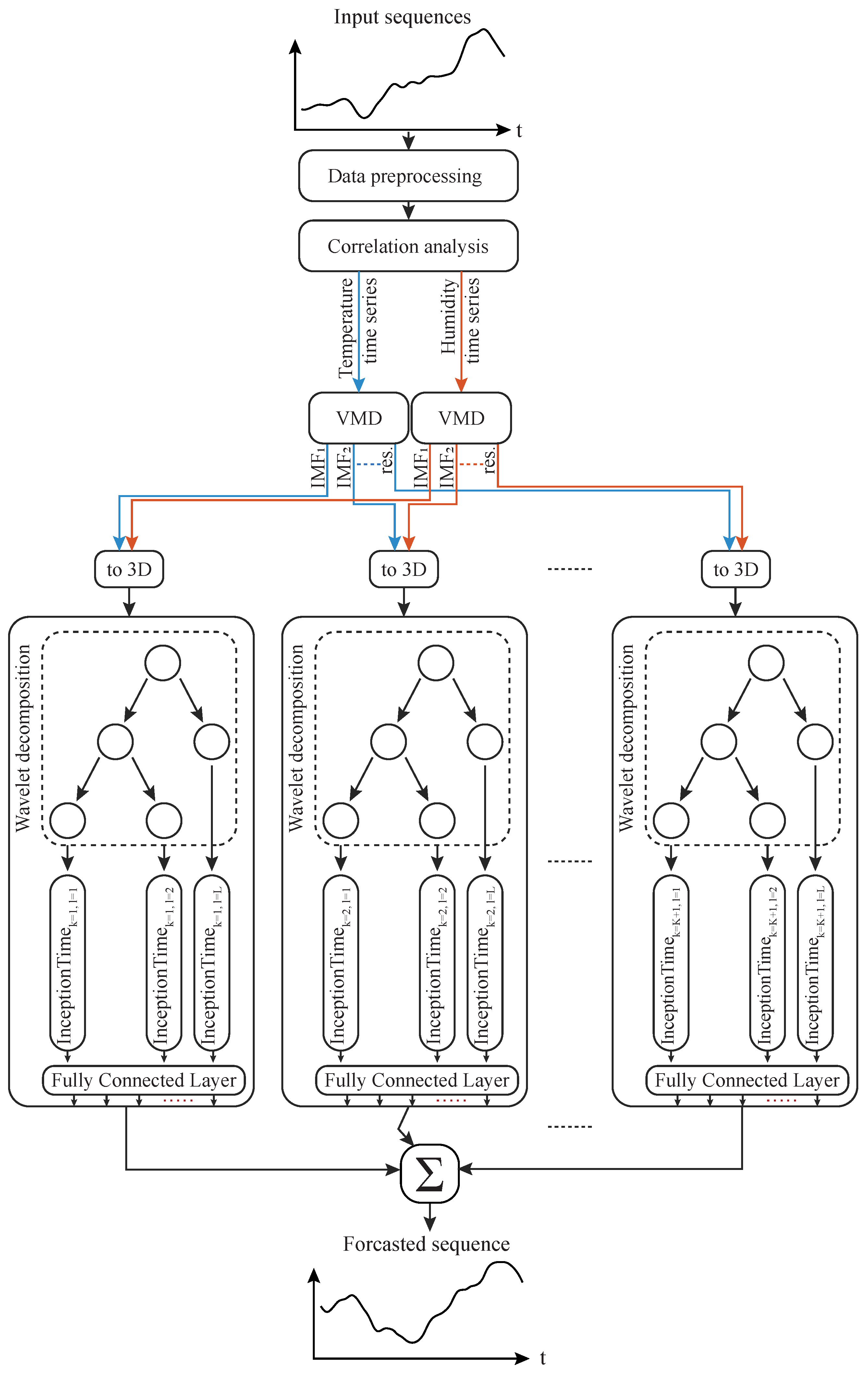
• Proposal of VMD-WT-InceptionTime for short-term multi-step air temperature forecasting. This hybrid technique is based on consecutive variational mode decomposition (VMD) and wavelet transform (WT) decompositions aiming to uncover hidden patterns and to reduce the complexity in past temperature and specific humidity sequences. These processed features are fed into a deep convolutional neural network forecasting model (InceptionTime).
• Comparison of the performance gains achieved through combined VMD and WT decompositions against using no decomposition or single decomposition techniques. To the best of the authors’ knowledge, the use of VMD and WT has not yet been investigated for the forecasting task at hand.
• Examination of the effects of VMD decomposition levels on the performance of the proposed forecasting technique and identification of the optimal level of decomposition.
• Assessment and validation of the technical experiments using multiple forecasting metrics and daily historical temperature data from three field sites in Alaska spanning 35+ years.

2. Background

2.1. Signal Decomposition Techniques

It is common practice to use signal decomposition techniques for time series analysis in order to remove noise and to capture inherent time-frequency information. Among the most commonly used time series decomposition methods are WT, empirical mode decomposition (EMD) [19], ensemble empirical mode decomposition (EEMD) [20], and VMD [21]. All these techniques have been successfully employed for diverse time series forecasting problems from financial market analysis [22,23,24], to earthquake and weather predictions [25,26], to machine health monitoring [27,28].

In general, WT provides a better alternative to Fourier transforms as it exhibits time-frequency localization characteristics [29]. However, its decomposition is strongly dependent on the choice of the basis wavelet function. EMD is an adaptive method that can decompose the signal according to the characteristics of the data itself without setting a basis function in advance [19]. However, it lacks an exact mathematical model and suffers from issues such as mode mixing and high sensitivity to noise. EEMD was proposed as an enhanced EMD to address noise and modal aliasing issues [20]. However, it requires a considerable amount of computation and can result in non-convergence. VMD was proposed as an alternative technique that can overcome such issues.

2.1.1. Variational Mode Decomposition

VMD is a mathematically framed non-recursive decomposition technique. It can simultaneously decompose the input time series into a discrete number of stationary and narrow-band sequences called intrinsic mode decompositions (IMF) [21]. The summation of all IMFs and the residue produces the original signal.

Let ${\left\{TS\left(t\right)\right\}}_{t=1}^H$ represent a certain non-stationary sequence of discrete values sampled over time. The decomposition of this time series using VMD can follow:

$$TS\left(t\right)=\sum _{m=1}^M{F}_m\left(t\right)+r\left(t\right)$$

(1)

where $F_m\left(t\right)$ is the extracted mth IMF sequence, M is the chosen decomposition level, and $r\left(t\right)$ is the residue.

Based on [21], an IMF is an amplitude-modulated and frequency-modulated signal following:

$$F_m\left(t\right)=A_m\left(t\right)cos{\varphi }_m\left(t\right),A_m\left(t\right)\ge 0$$

(2)

where ${\varphi }_m\left(t\right)$ is the phase and $A_m\left(t\right)$ is the slowly changing envelope corresponding to the mth $IMF$. It also has a non-decreasing instantaneous frequency that varies slowly and is mostly compact around a center frequency ${\omega }_m$.

Through use of the alternate direction method of multipliers (ADMM) optimization technique, VMD performs several computations to obtain the M IMFs and their corresponding central frequencies concurrently [30]. In particular, VMD can decompose the input $TS\left(t\right)$ into M$F_m$ and ${\omega }_m$ via ADMM using these equations [21]:

$$\mathcal{F}\left\{F_m^{n+1}\right\}=\frac{\mathcal{F}\left\{TS\left(\omega \right)\right\}-{\sum }_{i\ne m}\mathcal{F}\left\{F_i^{n+1}\left(\omega \right)\right\}+\frac{\mathcal{F}\left\{{\lambda }^n\left(\omega \right)\right\}}{2}}{1+2\alpha {(\omega -{\omega }_m^n)}^2}$$

(3)

$${\omega }_m^{n+1}=\frac{{\int }_0^{\infty }\omega {\left|\mathcal{F}\left\{F_m^{n+1}\left(\omega \right)\right\}\right|}^{2}d\omega }{{\int }_0^{\infty }{\left|\mathcal{F}\left\{F_m^{n+1}\left(\omega \right)\right\}\right|}^{2}d\omega }$$

(4)

where n is the number of iterations, $\lambda$ is the Lagrangian multiplier, and $\mathcal{F}\left\{F_m^{n+1}\right\}$, $\mathcal{F}\left\{TS\right(\omega \left)\right\}$, $\mathcal{F}\left\{F\right(\omega \left)\right\}$, and $\mathcal{F}\left\{{\lambda }^n\left(\omega \right)\right\}$ correspond to the Fourier transform of $F_m^{n+1}$, $TS\left(t\right)$, $F\left(t\right)$, and ${\lambda }^n$, respectively. The initial value of n, as well as of other parameters, ${\lambda }^1$, $\mathcal{F}\left\{F_m^1\right\}$, and ${\omega }_m^1$, are set to 0.

In comparison with other signal decomposition techniques, VMD differs from others, specifically with its level of decomposition M parameter. Therefore, it is essential to identify a suitable M for the given problem as choosing M at random may produce suboptimal decompositions due to noise and overlap.

2.1.2. Wavelet Decomposition

WT is an alternative technique to Fourier transforms in that it extracts local spectral and temporal information simultaneously with a window of variable width [31]. In this way, a local scale-dependent analysis of intricate patterns in the input time series can be performed.

The discrete WT decomposes an input signal into high- and low-frequency sequences (i.e., detail and approximation coefficients), which are further decomposed using the latter sub-series following a number of decomposition levels.

Let ${\left\{e_n^l\left(i\right)\right\}}_{n=1}^N$ and ${\left\{e_n^h\left(i\right)\right\}}_{n=1}^N$ denote the low and high sequences extracted from the input signal ${\left\{e\left(t\right)\right\}}_{t=1}^T$ in the ith decomposition level of a multilevel wavelet decomposition. Each sequence is generated using low- and high-pass filters $l=\{l_1,\dots ,l_M\}$, $h=\{h_1,\dots ,h_M\}$ followed by a downsampling technique (i.e., average pooling). Convolving $e^l\left(i\right)$ with l and h generates intermediate sequences ${\left\{a_n^l(i+1)\right\}}_{n=1}^{N/2}$ and ${\left\{a_n^h(i+1)\right\}}_{n=1}^{N/2}$ that can be expressed as:

$$a_n^l(i+1)=\sum _{m=1}^M{e}_{n+m-1}^l\left(i\right).l_m$$

(5)

$$a_n^h(i+1)=\sum _{m=1}^M{e}_{n+m-1}^l\left(i\right).h_m$$

(6)

where $e_n^l\left(i\right)$ is the nth element of $e_n^l\left(i\right)$, with $e_n^l\left(0\right)$ corresponding to the input of the model. The term $N/2$ refers to the 1/2 downsampling of the intermediate sequences. The final result of the WT comprises I detail sequences and a single approximation sequence. For the remainder of this paper, the Coiflets 6 wavelet function will be used to decompose the input time series.

2.2. InceptionTime

InceptionTime is a state-of-the-art time series classification model that was first introduced in 2019 [32] and has been investigated for different research problems [33,34,35]. The inception module serves as its main structural component. An inception module consists of (i) a bottleneck layer (one-dimensional convolutional layer) to reduce the dimensionality of the inputs, (ii) three one-dimensional convolutional layers with kernel sizes of 10, 20, and 40, which are fed the output of the bottleneck layer, (iii) the input of the inception module is also passed through a max pooling layer, (iv) the four convolutional layers’ outputs are concatenated along the depth dimension in the final layer, called a depth concatenation layer. Each inception module (i.e., convolutional layer) comes by default with 32 filters simultaneously applied to the input time series. To the best of the authors’ knowledge, this model has not yet been investigated for the task at hand.

2.3. Dataset Description and Study Locations

The Scenarios Network for Alaska and Arctic Planning (SNAP) dataset is a dynamically downscaled climate dataset containing historical and projected climate data for the state of Alaska and surrounding regions [36]. The SNAP dataset was created and is maintained by the International Arctic Research Center at the University of Alaska, Fairbanks. The dataset has a 20 km spatial resolution and daily temporal resolution covering the years from 1979 to 2015 (see

Table 1. Details of the SNAP dataset employed in this work.

Parameter	Value
Dataset	SNAP [36]
Temp. resolution	Daily
Spatial resolution	20 km
Time range	2 January 1979–29 October 2015
Number of samples	262 × 262 × 13,450
Features [Units]	Air temperature (T2) [K]
	Specific humidity (Q2) [kg/kg]
	Precipitation (PCPT) [mm]

for more details). Climate features found in the dataset are temperature, humidity, and precipitation measured two meters above the ground. The dataset was produced using the Weather Research and Forecasting model version 3.5. In this study, we employ all the available features over the period 1979–2015, spanning 35+ years.

According to the Government Accountability Office, over 30 Alaskan communities are imminently threatened by climate change and rising temperatures [37]. Three of these communities were selected as specific study regions: Nome, Bethel, and Utqiagvik (formerly known as Barrow). Figure 1a showcases the raw temperature time series plotted against time from each city with distinction between above- and below-freezing temperatures. Each of the three communities has additional characteristics that make them valuable study sites:

• Nome is located on the coast of the Bering Sea on the Seward Peninsula at a latitude of 64.5${}^{\prime }$ N and is in the discontinuous (50–90% permafrost coverage) permafrost zone [38]. Nome experiences a mean annual temperature of −2.2 ${}^{°}\mathrm{C}$, yet its position on the Bering Sea moderates the temperatures since the nearby large water mass provides thermal insulation from extreme air masses.
• Bethel is located on the Kuskokwim river in western Alaska 95 km inland from the mouth of the Kuskokwim River on the Bering Sea at a latitude of 60.8${}^{\prime }$ N. The mean annual air temperature of Bethel is $-0.3$ °C and it receives less temperature moderating influence from the Bering Sea than Nome due to its location nearly 100 km inland. The city is situated in the discontinuous permafrost zone [39] and is surrounded by many thermokarst lakes.
• Utqiagvik is the most northern study location at 71${}^{\prime }$ N and is situated on the Arctic Ocean in the continuous permafrost zone (>90% permafrost coverage) [40] with a mean annual air temperature of $-10.83$ ${}^{°}\mathrm{C}$.

Table 2. Descriptive statistics of the climate time series data from 1979 to 2015. The fluctuation frequency (FF) represents the percentage of instances with air temperature changes between two consecutive days succeeding or surpassing a certain threshold (minor fluctuations $\le 1K$ or rapid fluctuations $\ge 10K$). The stationarity of each time series is assessed using the augmented Dickey–Fuller (ADF) [41] and Kwiatkowski, Phillips, Schmidt, and Shin (KPSS) [42] tests. Both the raw T2 and the Q2 time series seem to be non-stationary.

Feature	Location	Stats					ADF		KPSS
		Mean	StD	Entropy	FF${}_{\le \mathbf{1}\mathit{K}}$	FF${}_{\ge \mathbf{10}\mathit{K}}$	Test Stat	cValue	Test Stat	cValue
T2	Nome	270.27	12.13	3.43	32.29%	1.29%	−0.080	−2.643	0.269	0.216
	Bethel	273.09	12.22	3.20	33.44%	2.39%	−0.073	−2.643	0.259	0.216
	Utqiagvik	262.34	13.75	3.49	32.21%	1.16%	−0.054	−2.643	0.251	0.216
Q2	Nome	0.003	0.002	2.929	-	-	−0.637	−2.643	0.253	0.216
	Bethel	0.004	0.002	3.128	-	-	−0.636	−2.643	0.235	0.216
	Utqiagvik	0.002	0.002	2.697	-	-	−0.694	−2.643	0.248	0.216
PCPT	Nome	1.486	3.427	0.609	-	-	−3.576	−2.643	0.122	0.216
	Bethel	1.841	3.309	0.982	-	-	−3.474	−2.643	0.108	0.216
	Utqiagvik	0.599	1.453	0.773	-	-	−3.680	−2.643	0.112	0.216

provides statistics of all the weather features found in this dataset, where the temperature and specific humidity raw sequences seem to be especially inherently complex and non-stationary in all three locations. In addition, all three locations exhibit a high frequency of minor daily temperature changes, with Bethel leading slightly, followed closely by Nome and Utqiagvik. On the other hand, extreme and rapid temperature variations do happen but at a significantly lower frequency and vary more between the locations, with Bethel showing the highest frequency. It is important to note that the primary goal of this paper is to demonstrate the effectiveness of the proposed hybrid forecasting technique within the specified experimental framework. While the SNAP dataset was used for proof of concept purposes, the proposed technique can still be investigated using alternative datasets or for other forecasting tasks.

3. Technical Implementation

This section focuses on the technical aspects of the study forecasting temperature in extremely cold regions. The proposed hybrid forecasting technique is described first. Figure 2 showcases its architecture. Then, three experiments are outlined that offer benchmarks and investigations of the impact of the different inputs, decomposition techniques, and deep learning models on the forecasting performance. The last subsection summarizes the benchmark models and how their performance is assessed throughout this study.

3.1. Temperature Forecasting Using the Proposed Technique

Let ${\left\{T\left(t\right)\right\}}_{t=1}^L$ denote the temperature sequence (of L samples) measured at the height of two meters. Multi-horizon forecasting of the temperature $T_{t-S+1|t}=\left\{T(t-S+1),\dots ,T\left(t\right)\right\}$, of $S-1$ elements and a time index t, can be written as:

$${\widehat{T}}_{t+S|t+1}=f\left(T_{t-L+1|t},ϵ\right)$$

(7)

where ${\widehat{T}}_{t+S|t+1}$ is the forecast temperature sequence over S-steps (i.e., horizons), f is the forecasting model, S is the horizon, L is the length of the input sequence, and $ϵ$ is the error.

Daily climate time series are processed to multivariate continuous sequences of $L+S$ in length, where the first L-elements represent the historical values (i.e., inputs), and the S-elements are the targeted future values (i.e., targets). This is performed using a sliding window of a unit stride. We consider different climate and time-related features:

• Temperature at two meters of height $T_{t-L+1|t}$: that provides direct historical temperature data.
• Humidity at two meters of height $Q_{t-L+1|t}$: to provide direct historical humidity data.
• Precipitation $P_{t-L+1|t}$: to provide direct historical precipitation data.
• Day of month: $D_{t-L+1|t}=\left\{D(t-L+1),\dots ,D\left(t\right)\right\}$ ranging from 1 to 31.
• Month of year: $M{o}_{t-L+1|t}=\left\{Mo(t-L+1),\dots ,Mo\left(t\right)\right\}$ ranging from 1 to 12.
• Year $Y_{t-L+1|t}=\left\{Y(t-L+1),\dots ,Y\left(t\right)\right\}$ ranging from 1979 to 2015.
• Season $S{e}_{t-L+1|t}=\left\{Se(t-L+1),\dots ,Se\left(t\right)\right\}$ ranging from 1 to 4, with 1 referring to winter, 2 to spring, 3 to summer, and 4 to fall.

Next, a Spearman correlation analysis ensues to select only the most correlated features to use for model learning. The resulting highly correlated features are then chronologically split into training and testing sets based on 80/20 ratios. Figure 3 showcases the rolling process followed to generate the continuous input–output sequences.

The VMD-processed temperature and specific humidity sequences in all the training and testing sets are standardized to have a zero mean and a unit standard deviation. This preprocessing step enables simplified computations and amplifies the forecasting model’s convergence speed. Accordingly, the forecast temperature sequences are reverse-standardized to provide the actual forecasts.

All data preprocessing is conducted using MATLAB 2023a. The parameters of VMD are set as follows. The penalty parameter is 1000, the number of IMFs is M (in addition to the residue), the initial center frequency is 0, and the convergence criterion is $5\times {10}^{-6}$.

3.2. Performance Evaluation

A number of inputs, forecasting models, and other cases are considered in order to validate the efficacy of the proposed hybrid model in forecasting the air temperature of the next seven days in Alaska.

3.2.1. Baseline Models

We consider five deep learning models for benchmark reasons: TST, the eXplainable Convolutional neural network for multivariate time series (XCM), LSTM, GRU, and the Miniature RandOm Convolutional KErnel Transform (MiniRocket). In addition, we employ six other statistical and conventional machine learning models as baselines. A brief description of each of these models follows:

• Historical mean: A simple baseline model relying on the values from the previous month (i.e., the last 30 elements) to provide short-term forecasts. Other variations of this model were considered (e.g., same week averaged over the past three months, same month averaged over the past three years), but the proposed historical model proved the best one.
• RF: It is an ensemble classifier that uses multiple decision trees to obtain a better prediction performance. A bootstrap technique is used to train each tree from the set of training data [43].
• GBDT [44]: It is an iterative ensemble model of multiple decision trees. In each iteration, GBDT learns the decision trees by fitting the negative gradients (also known as residual errors). The output of the GBDT is the accumulation of the outputs of all its component decision trees.
• SVR [45]: It is a popular conventional machine learning model for regression. In this work, we employ SVR with the sigmoid kernel.
• ARIMA [46]: It is a well-known statistical model for forecasting. ARIMA is generally applicable to non-stationary time series data. Its difference transformation can effectively transform non-stationary data into stationary data. In this work, we employ the Seasonal ARIMA model.
• TST [47]: It is a recent deep neural network that handles long-term dependencies while tracking relationships in sequential input to learn context and, subsequently, meaning. This model was initially proposed in 2017 for translation tasks for natural language processing in [48], but has now become a state-of-the-art model for various tasks in that field. Multihead-self-attention is the core component of TST that makes it suitable for processing time series data. This mechanism identifies multiple dynamic contextual information (i.e., past values, future values) of every element in a sequence, with every attention head. In the recent literature, attention-based deep learning has been effectively employed for uni- and multivariate time series forecasting problems [49,50,51].
• XCM [52]: It is a recently developed convolutional neural network that efficiently captures information related to both the observed variables and the timing of events directly from the input data, enabling it to have more robust and generalized learning on smaller and larger datasets.
• LSTM/GRU: LSTM is an RNN that is capable of learning long-term dependencies, especially in sequence prediction problems. It does this by introducing three gates known as the input gate, the forget gate, and the output gate that cooperate to control the information flow [53]. GRU was later introduced as a simpler alternative to LSTM, having its gating signal reduced to two (i.e., an update gate and a reset gate) and eliminating the need for distinguishing between memory cells and hidden states [54].
• MiniRocket [55]: It is a recent and computationally efficient alternative to the original ROCKET model while still achieving high performance on time series classification tasks. MiniRocket incorporates a series of random convolutional kernels to transform the input data into a high-dimensional feature space before feeding them to the classification or regression layer.

3.2.2. Model Hyper-Parameter Tuning

The considered deep learning models have multiple hyper-parameters that affect their learning process and overall performance. The use of non-optimal values can result in model under-performance. For this reason, several hyper-parameters of each one of these models were subject to optimization. In this work, the optimized hyper-parameters for InceptionTime include the use of a bottleneck layer, the number of filters, the kernel size, and the dropout rate at the convolution layer. For LSTM and GRU, the selected hyper-parameters to tune include the number of layers, the use of bias, the use of bidirectional layers, the dropout rate for the recurrent transformation, and the use of batch normalization. For TST, the tuned hyper-parameters include the number of features created by the model, the number of parallel attention heads, the activation function, the dimension of the feedforward network model, and the number of sub-encoder layers. For XCM, the hyper-parameters include the number of features, the use of batch normalization, and the window percentage. Finally, the tuned hyper-parameters of MiniRocket include the number of features, the kernel size, and the maximum number of kernels. In addition, the dropout rate at the final fully connected layer and the learning rate for all these models were also optimized.

As hyper-parameter tuning requires increased time and computational costs, all deep learning models were tuned for every location, under no decomposition, and with both temperature and humidity sequences. The tuned hyper-parameters from this case were used for the remaining cases (i.e., one or two decompositions, training using different inputs). The optimization trials were conducted using the Optuna framework [56] under the Tree-structured Parzen Estimator as the sampling algorithm for five epochs (with no early stopping) and 200 trials (with no pruning). The hyper-parameters of the proposed model are listed in

Table 3. Optimized hyper-parameters of the proposed model InceptionTime relative to Nome, Bethel, and Utqiagvik.

Hyper-Parameter			Nome	Bethel	Utqiagvik
Inception modules	Module number		6	6	6
	Bottleneck layer	filters	64	48	16
		kernel sizes	1	1	1
		stride	1	1	1
	Convolution layers	number of layers	3	3	3
		filters	64,64,64	48,48,48	16,16,16
		kernel sizes	39,19,9	19,9,5	79,39,19
		stride	1,1,1	1,1,1	1,1,1
		padding	19,9,4	9,4,2	39,19,9
	Max-pooling layer	kernel size	3	3	3
		stride	1	1	1
		padding	1	1	1
	Convolution layer	filters	64	48	16
		kernel size	1	1	1
		stride	1	1	1
	Concatenation layer	dimension	1	1	1
	Batch normalization	features	256	192	64
		momentum	0.1	0.1	0.1
	Dropout	p	32.3E-3	19.56E-5	7.6E-3
	Activation layer	function	ReLu	ReLu	ReLu
Optimizer			Adam	Adam	Adam
Loss function			Flattened MSE	Flattened MSE	Flattened MSE
Outputs			7	7	7
Epochs			30	30	30
Batch size			1024	1024	1024
Learning rate			30	30	30

.

3.2.3. Evaluation Metrics

The forecasting performance of all the developed models in this work is assessed using four metrics: RMSE, MAPE, $R^2$, and the mean directional accuracy (DA). RMSE assesses the mean square deviation of the forecasts. It is the main performance measure considered in this study as it is more sensitive to larger errors, which is critical in the context of the problem at hand. MAPE assesses the percentage of the mean absolute deviation between the forecast and the target. $R^2$ measures the proportion of variance in inputs that can be explained by the output. DA compares the forecast sequence direction (upward or downward) to the actual direction of the target sequence. This metric can be helpful in assessing the forecasting model in forecasting the thawing and freezing temperatures. The higher the values of RMSE and MAPE, the worse the model’s forecasting performance. The opposite is the case with the $R^2$ and DA metrics, where higher values refer to better performance.

These metrics are defined over all forecasting horizons following Equations (8)–(12):

$$\mathrm{RMSE}=\sqrt{\frac{1}{N\times S}\sum _{i=1}^N\sum _{h=1}^S{\left(y_i\left(h\right)-f_i\left(h\right)\right)}^2}$$

(8)

$$\mathrm{MAPE}=\frac{1}{N\times S}\sum _{i=1}^N\sum _{h=1}^S\left|\frac{y_i\left(h\right)-f_i\left(h\right)}{y_i\left(h\right)}\right|\times 100$$

(9)

$$R^2=1-\frac{{\sum }_{i=1}^N{\sum }_{h=1}^S{\left(y_i\left(h\right)-f_i\left(h\right)\right)}^2}{{\sum }_{i=1}^N{\sum }_{h=1}^S{\left(y_i\left(h\right)-{\overline{y}}_i\left(h\right)\right)}^2}$$

(10)

$$\mathrm{DA}=\frac{1}{N\times S}\times \sum _{i=1}^N\sum _{h=1}^S{P}_i\left(h\right)$$

(11)

$$P_i\left(h\right)=\left\{\begin{array}{cc}1\hfill & \mathrm{if}(y_{i+1}\left(h\right)-y_i\left(h\right))\times (f_{i+1}\left(h\right)-y_i\left(h\right))\ge 0\hfill \\ 0\hfill & \mathrm{otherwise}\hfill \end{array}\right.$$

(12)

where $y_i$ is the hth actual value of a test set sequence i, $f_i$ is the hth forecast value of the same test set sequence, N is the number of test set sequences, S is the number of horizons to be forecast ($S=7$), and $\overline{y}$ is the mean of $y_i$.

4. Results

4.1. Input Correlation Analysis

In this section, we investigate the correlation between various inputs and the output (i.e., forecasting target). Two types of input features were considered: climate features and time-related features. The first category of features comprises historical data of the temperature, humidity, and precipitation sequences, while the second holds historical data of the corresponding day of the month, the month of the year, the year, and the season. The latter features were extracted from the raw time series.

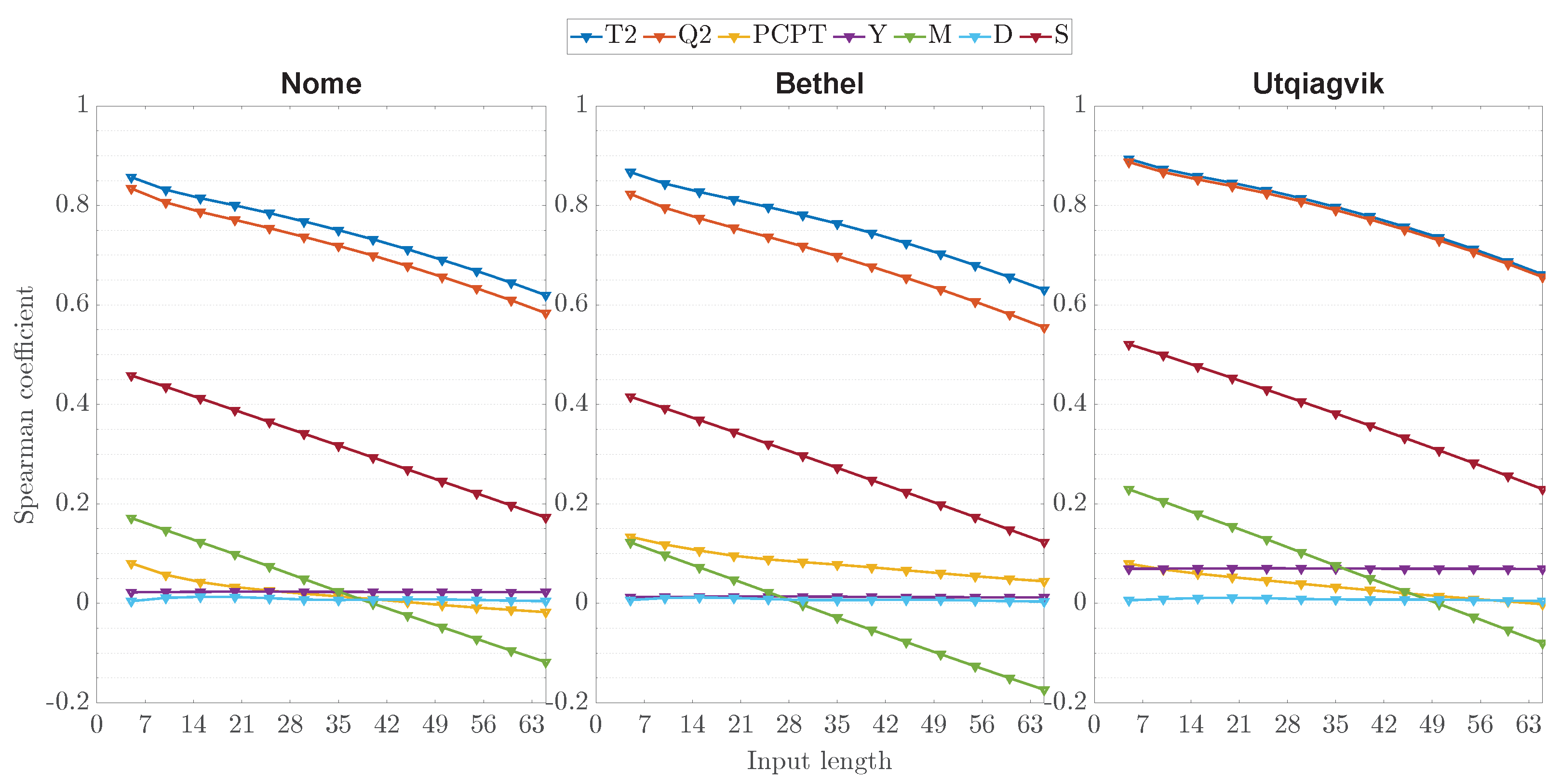
In addition, 10 different input sequence lengths (i.e., L) were considered to analyze the impact of the input lengths on the correlation with the output. We considered lengths ranging from the past five to 60 days with a five-day step.

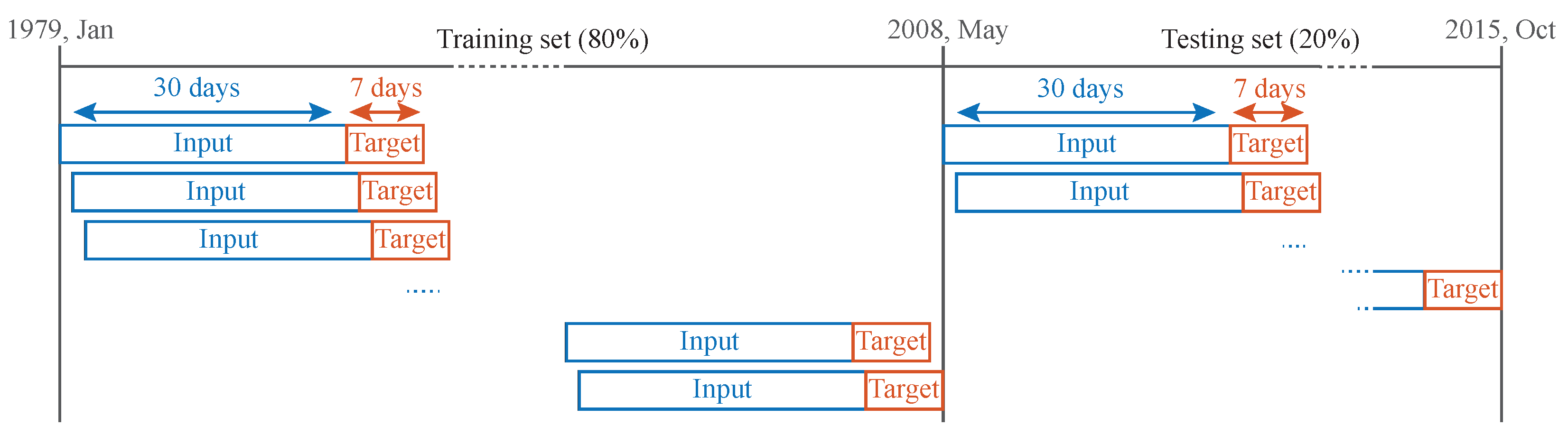
Figure 4 showcases the results of this study using the Spearman correlation algorithm. First, it is apparent that only the historical temperature and humidity are significantly correlated with the forecasting target sequences. For instance, average Spearman coefficients of $0.872$ and $0.848$ were identified for the temperature and humidity input sequences of $L=5$ days over all three locations. The other input features are either not correlated (e.g., year sequences) or slightly correlated with the targets (e.g., season, precipitation, and day sequences). Thus, it is reasonable to rely solely on the temperature and humidity sequences to forecast the near-future temperature values. Second, a higher correlation is seen with shorter input lengths. This is expected as these sequences can provide windows to the immediate past. With the increasing input lengths, their correlation with the targets decreases in the case of most features except for the month sequences, which seems to slightly increase its reverse correlation. Nevertheless, shorter sequences may not provide enough information to the forecasting model, leading to underperformance, while longer sequences require larger computational loads. Hence, the choice of using input sequences of $L=30$ elements (i.e., past 30 days) represents a good compromise between both aspects.

4.2. Decomposition Analysis

The notion of entropy serves as an indicator of the randomness and predictability of a system. Higher entropy signifies less order and more randomness. Time series’ regularity and complexity can be quantified by entropy measures such as the approximate entropy or, more recently, the sample entropy [57]. Although both parameters can reflect the predictability of a time series, the latter provides improved calculations and higher statistical accuracy than the former.

Table 4. Sample entropy computed using the Chebychev distance of three types of sequences: raw temperature (T2) and specific humidity (Q2) sequences, VMD decomposed ($M=15$) T2 and Q2 sequences, and WT decomposed ($I=3$) VMD sequences.

Input	Seq.	T2			Q2
		Nome	Bethel	Utqiagvik	Nome	Bethel	Utqiagvik
Raw TS	-	3.434	3.202	3.498	2.929	3.128	2.697
VMD(TS)	IMF1	0.873	1.009	1.004	0.99	1.109	1.092
	IMF2	0.973	0.964	0.987	1.001	0.999	1.005
	IMF3	0.652	0.653	0.651	0.667	0.676	0.654
	IMF4	0.449	0.443	0.435	0.437	0.42	0.431
	IMF5	0.289	0.266	0.278	0.282	0.279	0.3
	IMF6	0.203	0.212	0.189	0.205	0.214	0.222
	IMF7	0.174	0.173	0.171	0.174	0.18	0.186
	IMF8	0.163	0.18	0.169	0.16	0.157	0.171
	IMF9	0.168	0.163	0.177	0.179	0.181	0.174
	IMF10	0.164	0.164	0.188	0.19	0.171	0.189
	IMF11	0.165	0.17	0.186	0.175	0.175	0.175
	IMF12	0.16	0.157	0.163	0.17	0.193	0.175
	IMF13	0.103	0.112	0.095	0.11	0.116	0.11
	IMF14	0.024	0.025	0.02	0.027	0.023	0.021
	IMF15	0.053	0.052	0.055	0.018	0.021	0.018
	res.	0.283	0.271	0.279	0.267	0.286	0.275
WT(IMFx)	D1	0.446	0.4515	0.4575	0.4657	0.4726	0.4701
	D2	0.5371	0.5344	0.5446	0.5488	0.5579	0.555
	D3	0.5538	0.5569	0.5624	0.5797	0.5778	0.5698
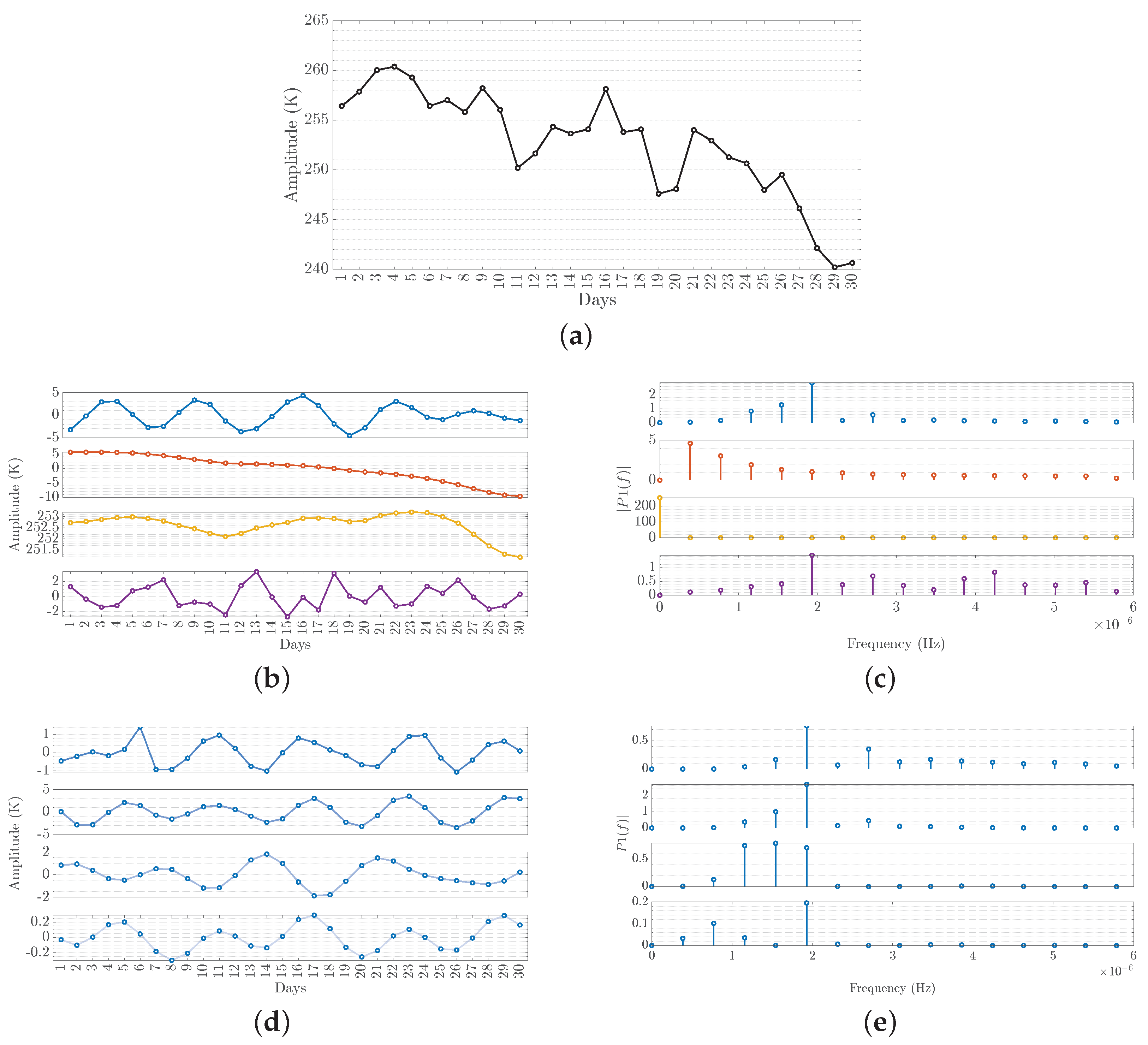
	A4	0.5612	0.5648	0.565	0.5797	0.5854	0.5834

presents the average sample entropy for the raw and decomposed T2 and Q2 sequences. Initially, the raw T2 sequences seem to reflect a high degree of complexity. Hence, further preprocessing seems necessary to produce simpler sequences for any subsequent processing. The decomposition using VMD proves capable of decreasing this complexity, where lower entropy values can be achieved with higher decomposition levels for both features. Decomposing every VMD decomposition (and residue) generates detail sequences (i.e., D1–D3) and an approximation sequence (i.e., A4) with lower complexity than those of the original IMFs. Hence, sequential decompositions of both the T2 and Q2 sequences can be useful in decreasing their complexity and ultimately improving the forecasting performance. These observations can be further seen in Figure 5 that showcases the VMD and WT decompositions of an input temperature sequence seen in Figure 5a. The raw time series is decomposed into $M=3$ decompositions, producing three IMFs and a residue. Figure 5b,c show the VMD resulting sequences of $M=3$ in their temporal and spectral representations, respectively. The proposed technique incorporates a second decomposition using WT (using the Coif6 wavelet function) that further decomposes each resulting VMD decomposition sequence (i.e., IMFs and residue). Similarly, Figure 5d,e show the WT resulting sequences of $I=3$ (i.e., three detail sequences and an approximation sequence) in their temporal and spectral representations, respectively. The residual sequences reflect the overall trend of the temperature time series.

4.3. Performance Benchmark

This section reports performance benchmarks between the proposed hybrid model and various forecasting models. The first benchmark is devised to demonstrate the validity of the proposed technique empowered by both VMD and WT in addressing the forecasting problem, compared with elementary versions of the same technique employing none or a single decomposition technique. The second benchmark is put forward to contextualize the proposed technique within a range of conventional and deep learning models.

Table 5. Overall air temperature forecasting performance averaged on the test set (best results in bold).

Case	Model	Nome				Bethel				Utqiagvik
		RMSE	MAPE	${\mathit{R}}^{\mathbf{2}}$	DA	RMSE	MAPE	${\mathit{R}}^{\mathbf{2}}$	DA	RMSE	MAPE	${\mathit{R}}^{\mathbf{2}}$	DA
No decomposition	InceptionTime	5.528	1.541	0.790	63.121	6.574	1.749	0.701	62.306	4.817	1.356	0.866	63.4
Single decomposition	WT + InceptionTime	5.286	1.486	0.808	64.192	5.6	1.513	0.783	64.699	4.6	1.307	0.878	63.9
	VMD + InceptionTime	0.798	0.214	0.995	90.648	0.809	0.205	0.995	91.261	0.739	0.202	0.996	91.2
Proposed technique	VMD + WT + InceptionTime	0.751	0.197	0.996	91.581	0.795	0.198	0.996	91.709	0.673	0.176	0.997	92.2

reports the average performances of the proposed technique and its elementary versions (i.e., with no decomposition and with a single decomposition) for all three field sites.

Table 6. Baseline models’ overall performance averaged on the test set (best results in bold).

Model	Nome				Bethel				Utqiagvik
	RMSE	MAPE	${\mathit{R}}^{\mathbf{2}}$	DA	RMSE	MAPE	${\mathit{R}}^{\mathbf{2}}$	DA	RMSE	MAPE	${\mathit{R}}^{\mathbf{2}}$	DA
Historical Mean	7.334	2.063	0.63	70.347	7.868	2.098	0.571	69.302	6.343	1.826	0.768	73.368
SVR-Sigmoid	12.083	3.79	−0.004	55.39	12.038	3.68	−0.004	54.122	13.25	4.487	−0.014	52.853
ExtraTrees	13.417	4.092	−0.238	55.129	16.88	4.845	−0.973	56.919	17.057	5.168	−0.68	55.017
GBDT	17.212	5.148	−1.037	58.896	16.907	4.855	−0.98	56.994	19.155	5.889	−1.119	58.448
RF	14.993	4.485	−0.546	55.054	16.963	4.876	−0.993	56.882	18.434	5.613	−0.962	57.367
SARIMAX	12.924	4.007	−0.149	54.569	11.928	3.638	0.015	55.651	13.142	4.396	0.003	53.115

and

Table 7. Performance comparison of the proposed technique against other deep learning models averaged on the test set (best results in bold).

Model	Nome				Bethel				Utqiagvik
	RMSE	MAPE	${\mathit{R}}^{\mathbf{2}}$	DA	RMSE	MAPE	${\mathit{R}}^{\mathbf{2}}$	DA	RMSE	MAPE	${\mathit{R}}^{\mathbf{2}}$	DA
TST	5.837	1.682	0.766	61.9	6.019	1.691	0.749	62.67	5.054	1.466	0.852	61.9
XCM	5.664	1.625	0.78	61.8	6.266	1.764	0.728	62.51	5	1.462	0.856	62.1
LSTM	6.061	1.757	0.747	60	6.539	1.857	0.704	61.38	5.656	1.671	0.815	59.8
GRU	6.112	1.761	0.743	60.2	6.285	1.773	0.727	62.41	5.42	1.595	0.83	60.1
MiniRocket	7.566	2.25	0.607	57	7.641	2.243	0.596	58.46	6.383	1.924	0.765	57.1
Proposed technique	0.751	0.197	0.997	91.6	0.795	0.198	0.996	91.71	0.673	0.176	0.997	92.2

provide the average performances of the baseline models’ and other deep learning models, respectively, for the three locations. The following observations can be gathered from the reported performances:

First, all the conventional machine learning and statistical forecasting models provide poorer forecasting performances than the historical mean model in terms of all the considered metrics. In particular, all the models clearly struggle to learn the complex fluctuations and trends in the temperature sequences. Nonetheless, the performance of the historical mean is not good enough, as is evident by the similarly low $R^2$ and DA scores achieved in all three locations (i.e., $R^2=63\%$ and $DA=70\%$ for Nome, $R^2=57\%$ and $DA=69\%$ for Bethel, and $R^2=76\%$ and $DA=73\%$ for Utqiagvik). However, the temperature at Utqiagvik seems to be slightly less challenging to forecast by this model as its average errors (i.e., RMSE and MAPE) are slightly better in this location than in the other two. In general, it is evident that the forecasting task is challenging since the patterns of the temperature sequences are evidently highly variable from week to week. This issue can be addressed with the incorporation of signal processing and deeper model architectures.

Indeed, better forecasting performances were achieved in all three field sites when employing a deep learning model (e.g., InceptionTime). In particular, deep learning models generally provided slightly better average performance than that of the historical mean model. In particular, training InceptionTime on undecomposed sequences reached average improvement rates of $24.63\%$, $25.30\%$, $-25.40\%$ in Nome, $16.45\%$, $16.63\%$, $-22.77\%$ in Bethel, and $24.06\%$, $25.74\%$, $-12.76\%$ in Utqiagvik, in terms of RMSE, MAPE, and $R^2$ when compared with the historical mean model. Slightly lower performances were generally found with the other deep learning models. For instance, TST achieved average improvement rates of $20.41\%$, $18.47\%$, $-21.59\%$ in Nome, $23.50\%$, $19.40\%$, $-31.17\%$ in Bethel, and $20.32\%$, $19.72\%$, $-10.94\%$ in Utqiagvik, respectively. However, these models reported lower performances in terms of AD than those achieved using the historical mean. In particular, InceptionTime reported average AD deterioration rates of $10.27\%$, $10.09\%$, $13.63\%$, while TST reported $12.03\%$, $9.57\%$, $15.63\%$, in all three locations, respectively. These results highlight the deep learning models’ inability to forecast the temperature’s trend. Thus, this simple approach of employing temperature sequences directly for deep model learning is ineffective.

Improved performances were obtained when incorporating a decomposition technique in the forecasting approach. Compared with the previous case (i.e., no decomposition), the processing temperature sequences using WT before model learning provided average improvement rates in all metrics of $4.38\%$, $3.57\%$, $-2.28\%$, $-1.7\%$ in Nome, $14.82\%$, $13.49\%$, $-11.7\%$, $-3.84\%$ in Bethel, and $4.5\%$, $3.61\%$, $-1.39\%$, $-0.89\%$ in Utqiagvik, respectively. However, this approach still seems to struggle in forecasting the next week’s trends, as its corresponding average DA score is less than 65% in all the considered field sites. Far greater improvements (compared to the same no decomposition case) were found in terms of all the metrics when incorporating VMD, with $84.90\%$, $85.60\%$, $-23.27\%$, $-41.21\%$ in Nome, $85.55\%$, $86.45\%$, $-27.08\%$, $-41.05\%$ in Bethel, and $83.93\%$, $84.54\%$, $-13.44\%$, $-42.59\%$ in Utqiagvik, respectively. These results prove the adequacy and necessity of decomposing the raw temperature time series first to provide the deep learning model with preprocessed and simpler temperature sequences.

The proposed technique, incorporating both decomposition techniques and the deep learning model, was the most accurate at forecasting the temperature in all three locations. Particularly when compared with the previous case (i.e., VMD only), the hybrid technique reported RMSE and MAPE average increase rates amounting to $5.89\%$ and $7.94\%$ in Nome, $1.73\%$ and $3.41\%$ in Bethel, and $8.39\%$, $12.87\%$ in Utqiagvik, respectively. Slight improvements were reported in the $R^2$ and $DA$ metrics, with rates of $-0.1\%$ and $-1.03\%$ in Nome, $-0.1\%$ and $-0.49\%$ in Bethel, and $-0.1\%$, $-1.18\%$ in Utqiagvik, respectively. The improved performance of the proposed hybrid technique over the VMD-only approach is likely due to the limitations of VMD in considering the temporal dimension of the time series. In particular, VMD decomposes the time series based on the Fourier spectrum, which does not take into account the temporal dimension of different frequencies. Hence, the incorporation of WT can accomplish such analysis on the already simplified input sequences (i.e., resulting IMFs from VMD) and more efficiently extract the inherent multi-resolution patterns, revealing temporal and spectral attributes simultaneously that are directly fed to the forecasting model for improved performance. In addition, similarly to the performances seen with the previous models and techniques, the lowest forecasting errors of the proposed technique among the considered field sites are achieved in Utqiagvik in terms of all the considered metrics. However, the proposed technique still has an average directional error (i.e., DA) lower than $93\%$, which means that the model can provide forecasts very close to the observed values but seems to struggle slightly in identifying their correct direction (i.e., increasing or decreasing temperature). This can be partly attributed to the training set from all locations having a smaller range of temperature values seen throughout the year, which would mean a smaller range of possible forecast values with higher minute differences between them. It is important to note that the other considered deep learning models were investigated using the decomposed inputs and achieved lower performances than those achieved using InceptionTime.

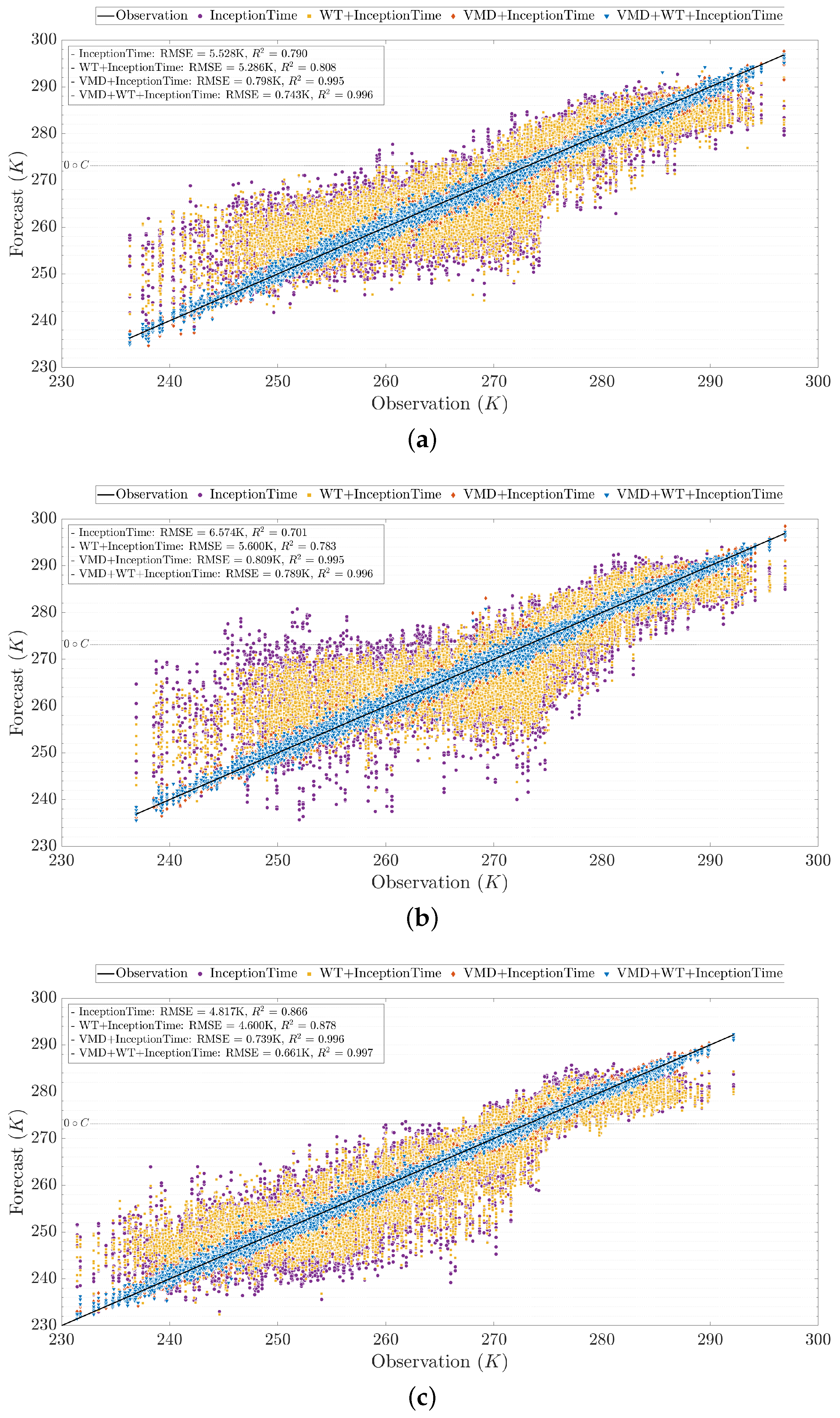
The superiority of the proposed hybrid technique compared to its elementary versions can be further showcased in the scatterplots in Figure 6, where it can be seen that the points (i.e., predictions) tend to get closer to the black line (i.e., observation) as signal decompositions are incorporated within the deep learning forecasting approach. The forecasts from the proposed technique (i.e., WVD+WT+InceptionTime) are the closest and fit the observed values the most.

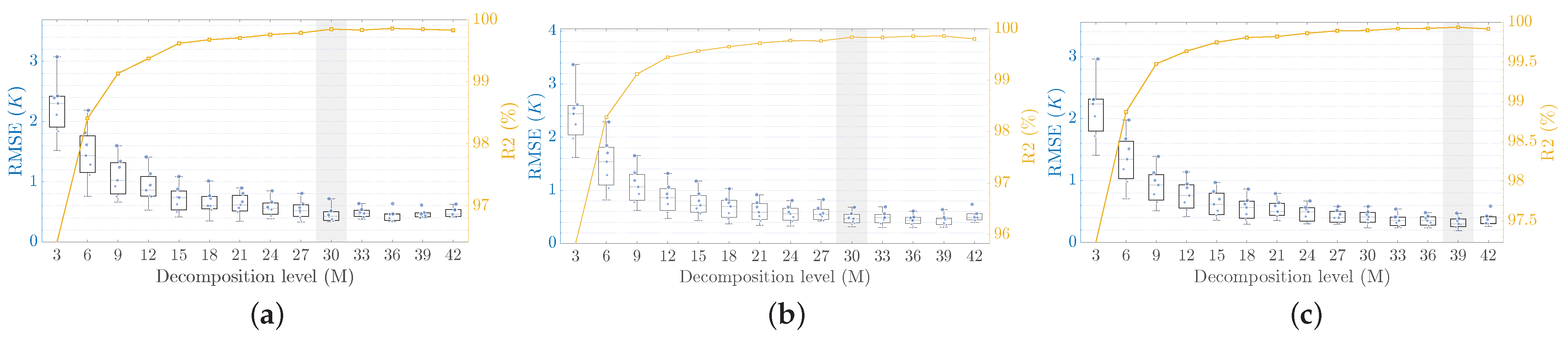
4.4. Impact of VMD Decomposition Level

Figure 7 showcases RMSE and $R^2$ boxplots computed using the proposed technique under VMD M values ranging from $M=3$ to $M=42$ with three-step increments. We note that only these two metrics are reported in the manuscript because the other two metrics provided a similar pattern.

As can be seen, the VMD decomposition level impacts the forecasting performance of the proposed model. The lowest forecasting performances in all three field sites are found using the lowest decomposition level of $M=3$. Under this configuration, the proposed model in Nome achieves an average RMSE score of $2.28K$ with a maximum value of $3.07K$ and a minimum of $1.51K$, while the average $R^2$ score is $96.41\%$. For Bethel, the average RMSE score is $2.45K$ with a maximum value of $3.36K$ and a minimum of $1.61K$, while the average $R^2$ score is $95.83\%$. For Utqiagvik, the average RMSE score is $2.23K$ with a maximum value of $2.96K$ and a minimum of $1.4K$, while the average $R^2$ score is $97.23\%$. Nevertheless, the proposed technique with lower M values still provides better average RMSE scores than all the other considered models and approaches. Enhanced performances can be achieved with higher values of M before either stagnating or worsening after a certain value. In particular, the average and the range of the RMSE scores are optimal at around $M=30$ for all Nome and Bethel measurements. For Utqiagvik, further improvements can be achieved with even higher values until $M=39$. In terms of $R^2$, the performance follows a similar pattern and stagnates at around the same M values. These improvements can be attributed to providing InceptionTime with less complex and more stationary sequences with highlighted multi-resolution intrinsic patterns.

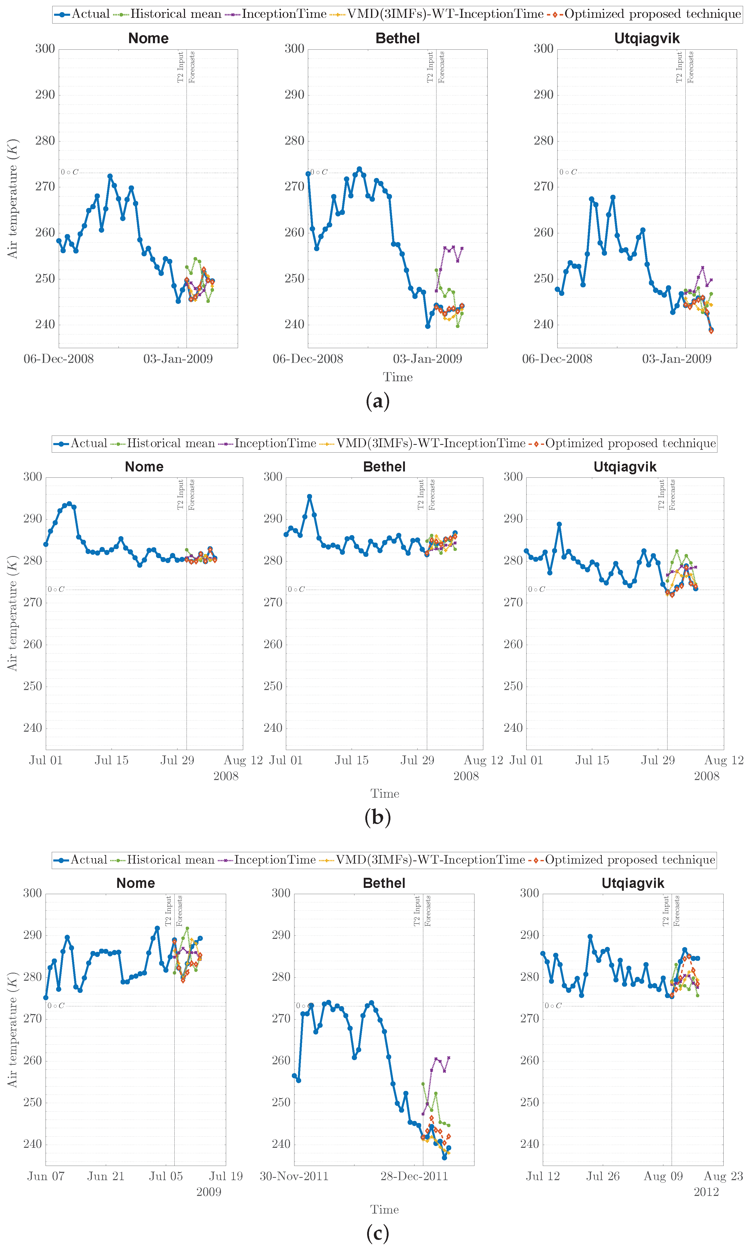
Figure 8 showcases examples of the input temperature sequences and their corresponding forecasts using the historical mean, InceptionTime (i.e., no decomposition), and the proposed technique under $M=30$ for Nome and Bethel, and $M=39$ for Utqiagvik, during the transition periods spanning different freezing and thawing periods. Specifically, Figure 8a,b present randomly selected sequences while Figure 8c displays the worst performance yielded by the proposed technique under the optimal M. In these plots, it is apparent that both versions of the proposed technique can follow the general trend of the observed temperature, with more accurate forecasts achieved under the optimal M for each location. Particularly, the proposed technique under $M=3$ seems to struggle to forecast abrupt and large changes in the temperature from one day to another. In contrast, the proposed technique under an optimal M seems to handle these variations more accurately.

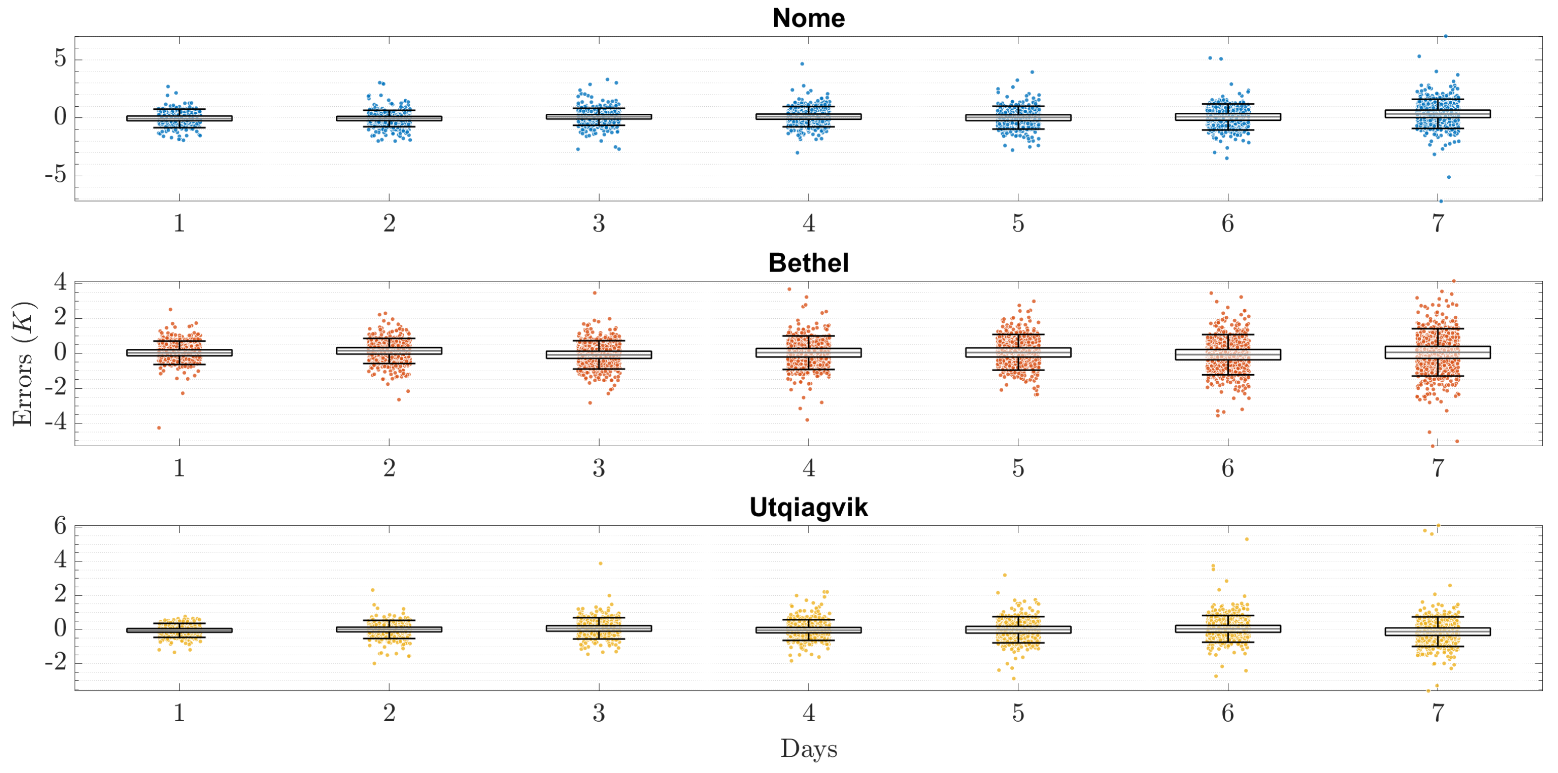
Further insights can be gathered from Figure 9, which reports a boxplot of per-horizon errors of the proposed technique employed using the optimal M for each of the three locations. First, it is apparent that the average errors at each horizon are very low. In particular, the optimized proposed technique for Nome produces forecasts over all seven horizons with a maximum error of $<1.6K$, a minimum error of $>-0.91K$, and an average error lower than $0.33K$; for Bethel, a maximum error of $<1.43K$, a minimum error of $>-1.29K$, and an average of $<0.05K$; and a maximum error of $<0.74K$, a minimum error of $>-0.99K$, and an average of $<-0.12K$ for Utqiagvik. Nonetheless, slightly higher errors can be seen with higher horizons. This can be attributed to the fact that the forecast uncertainties tend to increase as the horizons get further away in the future.

To better analyze the performance of the optimized proposed technique in handling challenging events, two analyses are conducted and reported. First,

Table 8. Top three air temperature forecasting errors produced by the optimized proposed technique (under $M=30$ for Nome and Bethel and $M=39$ for Utqiagvik).

Location	#	Error	Horiz.	Target Temperature Sequence
				Value	Range	Min.	Max.	Month
Nome	1st	−7.19	7	283.02	7.48	283.02	290.5	June
	2nd	5.16	6	288.34	9.37	280.01	289.38	June
	3rd	4.66	4	290.5	7.48	283.02	290.5	June
Bethel	1st	−5.3	7	268.33	15.22	257.69	272.91	March
	2nd	−4.26	1	265.19	11.57	258.25	269.82	February
	3rd	−3.81	4	250.63	22.88	247.64	270.52	January
Utqiagvik	1st	6.11	7	284.59	11.23	275.44	286.67	July
	2nd	5.3	6	265.03	20.32	244.72	265.03	November
	3rd	3.87	3	283.82	11.23	275.44	286.67	July

and

Table 9. Bottom three air temperature forecasting errors produced by the optimized proposed technique (under $M=30$ for Nome and Bethel and $M=39$ for Utqiagvik).

Location	#	Error	Horiz.	Target Temperature Sequence
				Value	Range	Min.	Max.	Month
Nome	1st	−0.0003	4	284.31	5.9	282.81	288.71	May
	2nd	−0.0002	7	276.5	5.16	276.5	281.66	April
	3rd	0.0001	6	281.33	3.83	279.21	283.04	April
Bethel	1st	0.0004	6	258.25	12.14	257.68	269.82	February
	2nd	−0.0001	4	270.62	8.14	268.5	276.64	February
	3rd	0.0001	7	282.33	6.52	282.33	288.85	July
Utqiagvik	1st	−0.0001	7	285.03	8.86	276.17	285.03	May
	2nd	−0.0001	5	266.95	5.96	265.26	271.21	September
	3rd	0.0001	3	232.97	11.49	232.97	244.46	December

report the horizon-wise top and bottom three errors from the testing set. It seems that the proposed technique’s lowest performances are errors of around $7K$ for Nome, $5K$ for Bethel, and $6K$ for Utqiagvik in the last horizon (i.e., 7th day). In particular, the worst performance of the optimized proposed technique corresponds to an overprediction for both Nome and Bethel and an underprediction for Utqiagvik. In addition, most of these errors are not related to the transition sequences between above- and below-freezing temperatures. Knowing that the average range, minimum, and maximum values in the target temperature sequences are $8.41K$, $266.64K$, and $275.05K$ in Nome, $8.51K$, $269.14K$, and $277.65K$ in Bethel, and $7.61K$, $260.43K$, $268.05K$ in Utqiagvik, most of the worst performances of the proposed technique in all three locations can be attributed to having to produce forecasts of higher variations and wider temperature ranges than the average. Indeed, most of the best performances of the proposed technique correspond to observed temperature sequences of ranges shorter than the average. Nevertheless, the proposed technique under the optimized M proves adequate and robust at forecasting the temperature at different periods of the year.

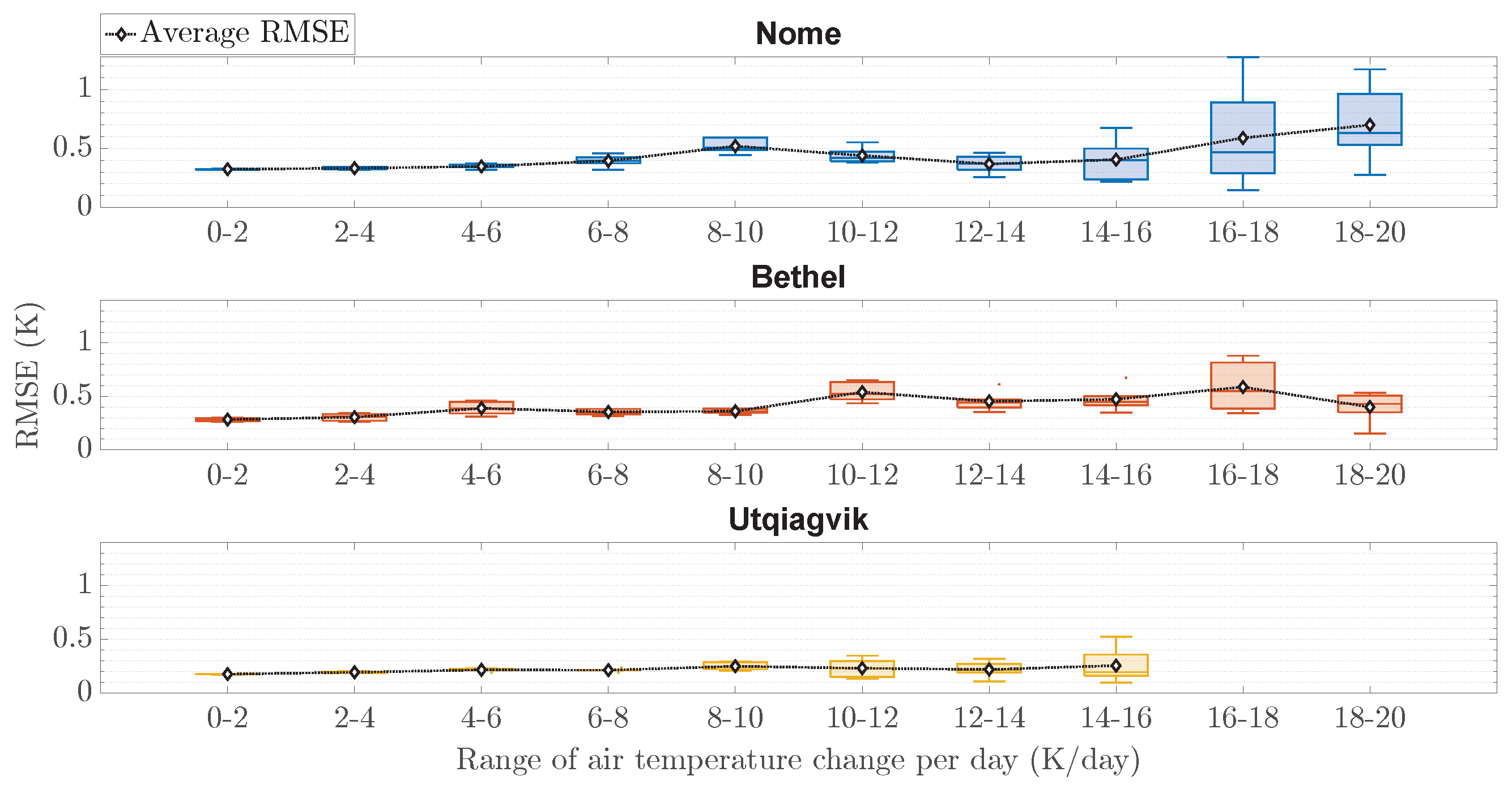
Second, Figure 10 showcases the RMSE distributions across different ranges of daily temperature spanning the whole testing set. The RMSE values were segmented into bins according to the magnitude of temperature change per day, allowing for an evaluation of the technique’s performance under varying conditions, ranging from low to rapid air temperature changes. Notably, the technique maintains generally low RMSE values across a wide range of daily temperature changes in all locations. Particularly in Bethel and Utqiagvik, the technique showcases consistent RMSE values across all ranges. However, increased RMSE variability can be seen with larger temperature changes in Nome, suggesting a slightly reduced forecast accuracy under extreme conditions. Nonetheless, the proposed technique under the optimized M proves adequate and robust even during instances of rapid fluctuations due to winter storms or other events.

5. Discussion

5.1. Preliminary Comparison with NOAA’s GFSv16

The Global Forecasting System version 16 (GFSv16) is the most recent generation of the National Atmospheric and Oceanic Administration’s (NOAA) numerical weather prediction models and is considered to be one of the premier numerical models for the forecasting of Earth’s surface air temperatures. The seven-day output from the proposed hybrid technique will be compared to that from the NOAA’s GFSv16 model. This comparison is conducted by utilizing the results of the 2021 GFSv16 model validation study that was undertaken before the GFSv16 was implemented into NOAA’s suite of weather models.

The data for this comparison are not readily available; hence, manual transcription of the graphics resulting from the study was undertaken to report approximate one-year RMSE values [58]. Manual transcription of the GFSv16 validation graphic was completed by first printing the graphic onto paper so that the central section of the figure with the plotted data points measured 20 cm in length along the x-axis. To tabulate the average RMSE, the highest relative points and the lowest relative points along the primary grouping of RMSE values for the given time period were sampled. To account for the difficulty of manually counting the points within the primary grouping, an estimated average of the RMSE for the grouping was made every 0.25 cm.

The calculation method used to manually transcribe the average RMSE from the GFSv16 validation graphic sampled 170 points (47.9% of the total points). However, this sampling method did not provide equal sampling along the full-year time series. A total of 57 of the 170 points were taken in the summer–mid-fall time period (i.e., late May to mid-October), achieving an average RMSE score of $3.29K$. Using the winter–spring period, accounting for 113 points, an average RMSE score of $5.57K$ was achieved. Since the summer–mid-fall period is under-sampled with respect to the winter–spring period, the two values were added in a weighted sum over their respective time periods to reach a final RMSE score of $4.64K$ for the whole one-year time series over all of northern Alaska. This value is significantly greater than the RMSE values found using the proposed hybrid technique, equating to an expected average improvement rate of 90% in terms of the RMSE, across the considered three locations.

5.2. Computational Costs

Due to the increasing number of sequences produced by VMD at higher decomposition levels, this search process can become increasingly computationally and time-intensive. Thus, it is crucial to select an appropriate increment value for the decomposition levels in order to demonstrate valuable changes in the technique’s performance and to limit the number of possibilities and associated costs. Additionally, the optimal decomposition level should be a compromise between performance improvement and the possible computational capabilities of the application in question. Nevertheless, the applicability of the proposed technique with $M=30$ or $M=39$ in real-world scenarios is feasible as the computational needs to both preprocess the data and to generate forecasts are inexpensive and timely, especially considering the forecasting granularity needed (i.e., a forecast every day).

5.3. Forecasting Using Different Combinations of Inputs

Different combinations of the five inputs considered in this work were investigated for air temperature forecasting using the proposed technique. However, the forecasting performance was generally lower or showed smaller improvements than that achieved using the past temperature and specific humidity as the sole inputs. These results corroborated the findings from the initial correlation analysis conducted between the inputs and the output sequences. Nonetheless, further enhancements in performance could still be achieved by investigating additional inputs and data sources (such as data used for determining atmospheric fronts and pressure systems). Despite the seeming limitation, the current results suggest that the proposed hybrid technique can still identify and learn the inherent patterns governed by natural processes and, hence, produce forecasts with small errors.

5.4. Forecasting the Air Temperatures under Rare Conditions

A data-driven approach such as deep learning for weather forecasting can be a powerful tool for better analyzing the input data and generating accurate forecasts. However, such techniques might be prone to yield lower performance than physics-based numerical models in certain relatively rare or unseen events, such as unusually fast moving low-pressure systems [59]. In these cases, numerical methods utilizing the advection–diffusion equation can prove beneficial in providing more accurate forecasts. In most cases, the best results are accomplished by ensemble forecasting methods that incorporate both machine learning and physics-based models [60], although resulting in higher computational costs and labor expenditure.

5.5. The Most Effective Use of the Findings

The most significant use of these findings may be for the forecasting of dangerously cold air temperatures during the winter season and for flood risk forecasting during the snow melt season. The study sites of Nome, Bethel, and Utqiagvik all experience extended episodes of dangerously low air temperatures that may cause cold-related harm to those caught without protection. Additionally, these predictions may allow for better forecasting of annual snow melt season flood risk.

6. Conclusions

In Alaska, accurate weather forecasts are critical for both human and economic vitality. Given the large computational costs of standard numerical models, a data-driven technique based on signal processing and deep learning is proposed to produce multi-horizon short-term local air temperature forecasts in Alaska. The integration of VMD and WT within the forecasting technique was shown to be able to extract hidden high- and low-frequency patterns within the raw time series that empowers the deep InceptionTime model to achieve superior forecasting performances (an average RMSE score of $0.42K$ over all three locations). The empirical results obtained highlighted the benefits of using the temperature and humidity sequences as well as a decomposition level of $M<40$ for VMD and $I=3$ for WT (coif6 wavelet function). The forecasting technique presented in this paper provided superior performances appropriate for the problem of short-term air temperature forecasting. Future work will focus on the same problem studied under long-term forecasting horizons, investigating different combinations of signal decomposition techniques.

References

1. Lawrence, D.M.; Slater, A.G. A projection of severe near-surface permafrost degradation during the 21st century. Geophys. Res. Lett. 2005, 32, L24401. [Google Scholar] [CrossRef]
2. Shen, X.; Wang, J.; Li, Z.; Chen, D.; Gong, J. Research and operational development of numerical weather prediction in China. J. Meteorol. Res. 2020, 34, 675–698. [Google Scholar] [CrossRef]
3. Thomas, G.; Mahfouf, J.F.; Montmerle, T. Toward a variational assimilation of polarimetric radar observations in a convective-scale numerical weather prediction (NWP) model. Atmos. Meas. Tech. 2020, 13, 2279–2298. [Google Scholar] [CrossRef]
4. Shin, Y.; Yi, C. Statistical downscaling of urban-scale air temperatures using an analog model output statistics technique. Atmosphere 2019, 10, 427. [Google Scholar] [CrossRef]
5. Cho, D.; Yoo, C.; Son, B.; Im, J.; Yoon, D.; Cha, D.H. A novel ensemble learning for post-processing of NWP Model’s next-day maximum air temperature forecast in summer using deep learning and statistical approaches. Weather Clim. Extrem. 2022, 35, 100410. [Google Scholar] [CrossRef]
6. DelSole, T.; Zhao, M.; Dirmeyer, P.A.; Kirtman, B.P. Empirical correction of a coupled land–atmosphere model. Mon. Weather Rev. 2008, 136, 4063–4076. [Google Scholar] [CrossRef]
7. Hou, Z.; Li, J.; Wang, L.; Zhang, Y.; Liu, T. Improving the forecast accuracy of ECMWF 2-m air temperature using a historical dataset. Atmos. Res. 2022, 273, 106177. [Google Scholar] [CrossRef]
8. Chen, K.; Wang, P.; Yang, X.; Zhang, N.; Wang, D. A model output deep learning method for grid temperature forecasts in Tianjin area. Appl. Sci. 2020, 10, 5808. [Google Scholar] [CrossRef]
9. Schultz, M.G.; Betancourt, C.; Gong, B.; Kleinert, F.; Langguth, M.; Leufen, L.H.; Mozaffari, A.; Stadtler, S. Can deep learning beat numerical weather prediction? Philos. Trans. R. Soc. A Math. Phys. Eng. Sci. 2021, 379, 20200097. [Google Scholar] [CrossRef]
10. Ayad, S. Modeling and forecasting air temperature in Tetouan (Morocco) using SARIMA model. J. Earth Sci. Geotech. Eng. 2022, 12, 1–13. [Google Scholar] [CrossRef]
11. Curceac, S.; Ternynck, C.; Ouarda, T.B.; Chebana, F.; Niang, S.D. Short-term air temperature forecasting using Nonparametric Functional Data Analysis and SARMA models. Environ. Model. Softw. 2019, 111, 394–408. [Google Scholar] [CrossRef]
12. Abhishek, K.; Singh, M.; Ghosh, S.; Anand, A. Weather forecasting model using artificial neural network. Procedia Technol. 2012, 4, 311–318. [Google Scholar] [CrossRef]
13. Ustaoglu, B.; Cigizoglu, H.; Karaca, M. Forecast of daily mean, maximum and minimum temperature time series by three artificial neural network methods. Meteorol. Appl. J. Forecast. Pract. Appl. Train. Tech. Model. 2008, 15, 431–445. [Google Scholar] [CrossRef]
14. Afzali, M.; Afzali, A.; Zahedi, G. The potential of artificial neural network technique in daily and monthly ambient air temperature prediction. Int. J. Environ. Sci. Dev. 2012, 3, 33. [Google Scholar] [CrossRef]
15. Fahimi Nezhad, E.; Fallah Ghalhari, G.; Bayatani, F. Forecasting maximum seasonal temperature using artificial neural networks “Tehran case study”. Asia-Pac. J. Atmos. Sci. 2019, 55, 145–153. [Google Scholar] [CrossRef]
16. Alomar, M.K.; Khaleel, F.; Aljumaily, M.M.; Masood, A.; Razali, S.F.M.; AlSaadi, M.A.; Al-Ansari, N.; Hameed, M.M. Data-driven models for atmospheric air temperature forecasting at a continental climate region. PLoS ONE 2022, 17, e0277079. [Google Scholar] [CrossRef]
17. Roy, D.S. Forecasting the air temperature at a weather station using deep neural networks. Procedia Comput. Sci. 2020, 178, 38–46. [Google Scholar] [CrossRef]
18. Nandi, A.; De, A.; Mallick, A.; Middya, A.I.; Roy, S. Attention based long-term air temperature forecasting network: ALTF Net. Knowl. Based Syst. 2022, 252, 109442. [Google Scholar] [CrossRef]
19. Huang, N.E.; Shen, Z.; Long, S.R.; Wu, M.C.; Shih, H.H.; Zheng, Q.; Yen, N.C.; Tung, C.C.; Liu, H.H. The empirical mode decomposition and the Hilbert spectrum for nonlinear and non-stationary time series analysis. Proc. R. Soc. Lond. Ser. A Math. Phys. Eng. Sci. 1998, 454, 903–995. [Google Scholar] [CrossRef]
20. Wu, Z.; Huang, N.E. Ensemble empirical mode decomposition: A noise-assisted data analysis method. Adv. Adapt. Data Anal. 2009, 1, 1–41. [Google Scholar] [CrossRef]
21. Dragomiretskiy, K.; Zosso, D. Variational Mode Decomposition. IEEE Trans. Signal Process. 2014, 62, 531–544. [Google Scholar] [CrossRef]
22. Kulaglic, A.; Üstündağ, B.B. Stock price forecast using wavelet transformations in multiple time windows and neural networks. In Proceedings of the 2018 3rd IEEE International Conference on Computer Science and Engineering (UBMK), Sarajevo, Bosnia and Herzegovina, 20–23 September 2018; pp. 518–521. [Google Scholar]
23. Peng, L.; Chen, K.; Li, N. Predicting stock movements: Using multiresolution wavelet reconstruction and deep learning in neural networks. Information 2021, 12, 388. [Google Scholar] [CrossRef]
24. Ali, M.; Khan, D.M.; Alshanbari, H.M.; El-Bagoury, A.A.A.H. Prediction of complex stock market data using an improved hybrid emd-lstm model. Appl. Sci. 2023, 13, 1429. [Google Scholar] [CrossRef]
25. Xing, Y.; Yue, J.; Chen, C.; Cong, K.; Zhu, S.; Bian, Y. Dynamic displacement forecasting of dashuitian landslide in China using variational mode decomposition and stack long short-term memory network. Appl. Sci. 2019, 9, 2951. [Google Scholar] [CrossRef]
26. Li, G.; Ma, X.; Yang, H. A hybrid model for monthly precipitation time series forecasting based on variational mode decomposition with extreme learning machine. Information 2018, 9, 177. [Google Scholar] [CrossRef]
27. Duarte, D.; Walshaw, C.; Ramesh, N. A comparison of time-series predictions for healthcare emergency department indicators and the impact of COVID-19. Appl. Sci. 2021, 11, 3561. [Google Scholar] [CrossRef]
28. Chen, P.; Deng, Y.; Zhang, X.; Ma, L.; Yan, Y.; Wu, Y.; Li, C. Degradation trend prediction of pumped storage unit based on MIC-LGBM and VMD-GRU combined model. Energies 2022, 15, 605. [Google Scholar] [CrossRef]
29. Akin, M. Comparison of wavelet transform and FFT methods in the analysis of EEG signals. J. Med Syst. 2002, 26, 241–247. [Google Scholar] [CrossRef]
30. Boyd, S.; Parikh, N.; Chu, E.; Peleato, B.; Eckstein, J. Distributed Optimization and Statistical Learning via the Alternating Direction Method of Multipliers. Found. Trends Mach. Learn. 2011, 3, 1–122. [Google Scholar] [CrossRef]
31. Addison, P.S. Wavelet transforms and the ECG: A review. Physiol. Meas. 2005, 26, R155. [Google Scholar] [CrossRef]
32. Ismail Fawaz, H.; Lucas, B.; Forestier, G.; Pelletier, C.; Schmidt, D.F.; Weber, J.; Webb, G.I.; Idoumghar, L.; Muller, P.A.; Petitjean, F. InceptionTime: Finding AlexNet for time series classification. Data Min. Knowl. Discov. 2020, 34, 1936–1962. [Google Scholar] [CrossRef]
33. Zhou, K.; Wang, W.; Hu, T.; Deng, K. Time series forecasting and classification models based on recurrent with attention mechanism and generative adversarial networks. Sensors 2020, 20, 7211. [Google Scholar] [CrossRef] [PubMed]
34. Guo, F.; Li, W.; Jiang, P.; Chen, F.; Liu, Y. Deep learning approach for damage classification based on acoustic emission data in composite materials. Materials 2022, 15, 4270. [Google Scholar] [CrossRef]
35. Wang, P.; Wu, J.; Wei, Y.; Li, T. CEEMD-MultiRocket: Integrating CEEMD with Improved MultiRocket for Time Series Classification. Electronics 2023, 12, 1188. [Google Scholar] [CrossRef]
36. Bieniek, P.A. Downscaled Climate Data for Alaska; Technical Report; International Arctic Research Center, University of Alaska Fairbanks: Fairbanks, AK, USA, 2019; Available online: https://registry.opendata.aws/wrf-alaska-snap (accessed on 26 June 2023).
37. Mittal, A.K. Alaska Native Villages: Limited Progress Has Been Made on Relocating Villages Threatened by Flooding and Erosion; DIANE Publishing: Collingdale, PA, USA, 2009. [Google Scholar]
38. Debolskiy, M.; Nicolsky, D.; Hock, R.; Romanovsky, V. Modeling present and future permafrost distribution at the Seward Peninsula, Alaska. J. Geophys. Res. Earth Surf. 2020, 125, e2019JF005355. [Google Scholar] [CrossRef]
39. Zhao, Y.; Yang, Z.J. Historical and long-term climate trends in warm permafrost regions: A case study of Bethel, AK. Cold Reg. Sci. Technol. 2022, 204, 103677. [Google Scholar] [CrossRef]
40. Brewer, M.C. Some results of geothermal investigations of permafrost in northern Alaska. Eos Trans. Am. Geophys. Union 1958, 39, 19–26. [Google Scholar]
41. SAID, S.E.; DICKEY, D.A. Testing for unit roots in autoregressive-moving average models of unknown order. Biometrika 1984, 71, 599–607. [Google Scholar] [CrossRef]
42. Kwiatkowski, D.; Phillips, P.C.; Schmidt, P.; Shin, Y. Testing the null hypothesis of stationarity against the alternative of a unit root: How sure are we that economic time series have a unit root? J. Econom. 1992, 54, 159–178. [Google Scholar] [CrossRef]
43. Ho, T.K. Random decision forests. In Proceedings of the 3rd IEEE International Conference on Document Analysis and Recognition, Montreal, QC, Canada, 14–16 August 1995; Volume 1, pp. 278–282. [Google Scholar]
44. Friedman, J.H. Greedy function approximation: A gradient boosting machine. Ann. Stat. 2001, 29, 1189–1232. [Google Scholar] [CrossRef]
45. Drucker, H.; Burges, C.J.; Kaufman, L.; Smola, A.; Vapnik, V. Support vector regression machines. In Proceedings of the NIPS’96: Proceedings of the 9th International Conference on Neural Information Processing Systems, Denver, CO, USA, 2–5 December 1996. [Google Scholar]
46. Newbold, P. ARIMA model building and the time series analysis approach to forecasting. J. Forecast. 1983, 2, 23–35. [Google Scholar] [CrossRef]
47. Zerveas, G.; Jayaraman, S.; Patel, D.; Bhamidipaty, A.; Eickhoff, C. A Transformer-Based Framework for Multivariate Time Series Representation Learning. In Proceedings of the 27th ACM SIGKDD Conference on Knowledge Discovery & Data Mining (KDD ’21), New York, NY, USA, 14–18 August 2021; pp. 2114–2124. [Google Scholar] [CrossRef]
48. Vaswani, A.; Shazeer, N.; Parmar, N.; Uszkoreit, J.; Jones, L.; Gomez, A.N.; Kaiser, Ł.; Polosukhin, I. Attention is all you need. In Proceedings of the 31st Conference on Neural Information Processing Systems (NIPS 2017), Long Beach, CA, USA, 4–9 December 2017. [Google Scholar]
49. Lara-Benítez, P.; Gallego-Ledesma, L.; Carranza-García, M.; Luna-Romera, J.M. Evaluation of the Transformer Architecture for Univariate Time Series Forecasting. In Proceedings of the Conference of the Spanish Association for Artificial Intelligence; Springer: Cham, Switzerland, 2021; pp. 106–115. [Google Scholar]
50. Hu, Y.; Xiao, F. Network self attention for forecasting time series. Appl. Soft Comput. 2022, 124, 109092. [Google Scholar] [CrossRef]
51. He, X.; Shi, S.; Geng, X.; Xu, L. Dynamic Co-Attention Networks for multi-horizon forecasting in multivariate time series. Future Gener. Comput. Syst. 2022, 135, 72–84. [Google Scholar] [CrossRef]
52. Fauvel, K.; Lin, T.; Masson, V.; Fromont, É.; Termier, A. Xcm: An explainable convolutional neural network for multivariate time series classification. Mathematics 2021, 9, 3137. [Google Scholar] [CrossRef]
53. Hochreiter, S.; Schmidhuber, J. Long short-term memory. Neural Comput. 1997, 9, 1735–1780. [Google Scholar] [CrossRef]
54. Cho, K.; Van Merriënboer, B.; Gulcehre, C.; Bahdanau, D.; Bougares, F.; Schwenk, H.; Bengio, Y. Learning phrase representations using RNN encoder-decoder for statistical machine translation. arXiv 2014, arXiv:1406.1078. [Google Scholar]
55. Dempster, A.; Schmidt, D.F.; Webb, G.I. MiniRocket: A Very Fast (Almost) Deterministic Transform for Time Series Classification. In Proceedings of the 27th ACM SIGKDD Conference on Knowledge Discovery and Data Mining, New York, NY, USA, 14–18 August 2021; pp. 248–257. [Google Scholar]
56. Akiba, T.; Sano, S.; Yanase, T.; Ohta, T.; Koyama, M. Optuna: A Next-generation Hyperparameter Optimization Framework. In Proceedings of the 25rd ACM SIGKDD International Conference on Knowledge Discovery and Data Mining, Anchorage, AK, USA, 4–8 August 2019; pp. 2623–2631. [Google Scholar]
57. Pincus, S.M.; Goldberger, A.L. Physiological time-series analysis: What does regularity quantify? Am. J. Physiol. Heart Circ. Physiol. 1994, 266, H1643–H1656. [Google Scholar] [CrossRef]
58. Levitt, J.; Row, M.; Tallapragada, V.; Adimi, F.; Yang, F.; Treadon, R. GFSv16 Verification. National Oceanic and Atmospheric Administration; 2021. Available online: https://emc.ncep.noaa.gov/users/verification/global/gfs/gfsv16/grid2obs/rmse (accessed on 1 January 2024).
59. Parker, C.L.; Mooney, P.A.; Webster, M.A.; Boisvert, L.N. The influence of recent and future climate change on Spring Arctic Cyclones. Nat. Commun. 2022, 13, 6514. [Google Scholar] [CrossRef]
60. Arcomano, T.; Szunyogh, I.; Wikner, A.; Pathak, J.; Hunt, B.R.; Ott, E. A hybrid approach to atmospheric modeling that combines machine learning with a physics-based numerical model. J. Adv. Model. Earth Syst. 2022, 14, e2021MS002712. [Google Scholar] [CrossRef]
Figure 1. Data from the SNAP dataset [36] from three field sites in Nome, Bethel, and Utqiagvik in Alaska. (a) Daily temperature time series over time with distinctions between freezing and thawing temperatures; (b) Map of the three field sites in Alaska.
Forecasting 06 00004 g001
Figure 2. Multi-horizon forecasting of the temperature using VMD-WT-InceptionTime.
Forecasting 06 00004 g002
Figure 3. Moving window schematic to construct training and testing sets. The testing set period spans between 21 May 2008 and 29 October 2015.
Forecasting 06 00004 g003
Figure 4. Spearman correlation results between different inputs and the target output for every location. Different input lengths were considered for each input feature spanning nine weeks.
Forecasting 06 00004 g004
Figure 5. Example of temperature sequences sequentially processed using VMD ( M = 3 ) and WT ( I = 3 ). (a) Raw temperature sequence; (b) Resulting VMD decomposed sequences from the temperature sequence; (c) Single-sided amplitude spectrum of the VMD decomposed sequences; (d) Resulting WT decomposed sequences from a single IMF; (e) Single-sided amplitude spectrum of WT decomposed sequences.
Forecasting 06 00004 g005
Figure 6. Scatterplots comparing observed and forecast air temperatures in the three field sites using InceptionTime under four approaches: no decomposition, WT decomposition only, VMD only, and the proposed hybrid VMD-WT technique. (a) Nome; (b) Bethel; (c) Utqiagvik.
Forecasting 06 00004 g006
Figure 7. Impact of different VMD decomposition levels on the average performance of the proposed hybrid model on the test set in terms of RMSE and R 2 . (a) Nome; (b) Bethel; (c) Utqiagvik.
Forecasting 06 00004 g007
Figure 8. Examples of air temperature forecasts using the optimized proposed forecasting technique ( M = 30 for Nome and Bethel and M = 39 for Utqiavik) compared with actual measurements from the test set. Additional forecasts using the proposed technique under a sub-optimal decomposition level (M = 3), no decomposition using InceptionTime, and the historical means are shown for reference. All plots share the same vertical axis limits for comparison reasons. (a) randomly selected sequences. (b) randomly selected sequences. (c) the worst performance.
Forecasting 06 00004 g008
Figure 9. Boxplot of per-horizon errors found using the optimized proposed technique under M = 30 for Nome and Bethel and under M = 39 for Utqiagvik on the testing sets.
Forecasting 06 00004 g009
Figure 10. RMSE performance distribution of the optimized forecasting technique, segmented by the range of daily air temperature changes. The forecast and observation sequences were binned into intervals of 2 K by computing the amplitude change between consecutive pairs of days (K/day). It is noteworthy that even under rapid air temperature fluctuations, the technique is capable of producing forecasts with low RMSE values at all three locations.
Forecasting 06 00004 g010