1. Introduction
Computational fluid dynamics (CFD) is a powerful tool for studying blood flow in different parts of the vascular bed and can account for such factors as geometry complexity, vessel wall elasticity, blood rheology, and turbulence [
1]. Compared to measurements, up-to-date numerical simulations of blood flow provide significantly more information about the velocity and pressure fields, as well as wall shear stresses. Obtained information in some cases is used for diagnosing blood flow disorders and for the planning of operations.
Modern technologies in CFD implement numerical methods that make it possible to simulate viscous fluid flows in areas of arbitrary, often rather complex, geometry; bifurcations of blood vessels are also in this row. This opportunity has arisen due to the intensive development of numerical methods known as the finite element method (FEM) and the finite volume method (FVM). Both of these methods belong to the class of mesh-based methods, but use different approaches to obtain algebraic systems that approximate the basic partial differential equations of continuum mechanics. The FEM method is especially in demand for solving problems of structural mechanics. Regarding fluid dynamic problems, the fundamental conservation property of the FVM makes it the preferable method in comparison to the FEM, and the FVM is currently the most widely used numerical technique for CFD studies.
The FVM is based on the approximate solution of the integral form of the conservation equations. The computational domain chosen for the investigated problem is divided into a set of non-overlapping control volumes referred to as finite volumes, where the variables of interest are assigned to the center of the finite volume. The finite volume is also referred to as a cell or element, and can be of different forms: tetrahedral, prismatic, hexahedral, and polyhedral. The governing equations are integrated over each finite volume, and some interpolation procedures are assumed, which serve to restore representative values of the variable of interest at the faces of the current cell by making up some combination of the central value and values from the centers of neighboring cells. The resulting discretization (algebraic) equation expresses with a specified order of accuracy the conservation principle for the variable inside the finite volume, and the system of such equations is to be solved using some algorithm, usually iterative. When solving time-dependent problems, the time derivative of the variable of interest is approximated for the center of the cell using one or another finite-difference scheme, and iterative calculations with discrete time steps are carried out sequentially at different time steps. In the case of 3D incompressible viscous fluid flows, the governing equations are the Navier–Stokes equations and the continuity equation, and the variables of interest are pressure and three components of the velocity vector. A detailed description of the numerical schemes and algorithms most widely used to solve problems of incompressible viscous fluid dynamics can be found elsewhere [
2,
3].
Blood flow studies in various vessels, healthy and damaged, as well as in vascular prostheses, are often carried out using simplified models, for the construction of which average statistical data are used. This approach makes it possible to conduct extended parametric studies, test new experimental methods for clinical diagnosis of blood flow in phantoms, and validate CFD methods under conditions of complex transient flow regimes. From the other side, the progress of computing tools has opened up the possibility of the widespread use of personalized vascular models in both pre- and post-operative settings. This approach allows for the individual selection of a prosthesis and surgical technique [
4,
5,
6].
In the natural vessel bifurcations, a complex spatial structure of blood flow is formed, which in some cases is one of the causes of atherosclerotic changes in the vessel wall [
7]. Significant disturbances in the physiological structure of blood flow are also observed in the areas of vessels’ connection with synthetic prostheses of the “end-to-side” type, namely, in the areas of proximal and distal anastomoses. It can lead to neointimal hyperplasia, thrombosis of prostheses, and their complete blockage, requiring reoperation [
8,
9].
When studying the blood flow patterns in anastomoses, numerical modeling is wildly used, the results of which in some cases are compared with experimental data [
10]. Most in vitro studies in anastomotic models for femoral popliteal bypass surgery were performed using particle image velocimetry (PIV) [
11]. A recent experience in using the smoke image velocimetry (SIV) measurement technique for studying fluid motion with local turbulence in a proximal anastomosis model is presented in [
12]. Ultrasound (US) methods for blood flow analysis are used mainly in clinical studies [
13]. To obtain knowledge that is useful for the early prediction of dangerous postoperative complications, numerical calculations are performed for personalized anastomosis models based on magnetic resonance imaging (MRI) [
14], US and multispiral computed tomography (MSCT) data [
15,
16,
17].
In the case of numerical simulations of blood flow using personalized models for one or another part of the vascular bed, the problem of the incomplete definition of boundary conditions always arises, resulting from the difficulties of clinical blood flow measurements. Accordingly, it is necessary to introduce some assumptions. Sometimes, numerical results are supplemented by an uncertainty analysis, and for greater reliability, the calculation results are compared with US measurements. The authors of several works dealing with studies of complex blood flows clearly give preference to US methods in terms of accuracy and involve US data to validate the CFD results [
18,
19]. On the other side, the data reported in other works allows one to conclude that in the case of personalized blood flow studies, numerical modeling and ultrasound measurements provide results of comparable accuracy [
20,
21].
Nowadays, US methods remain the leader among clinical methods for blood flow diagnostics, despite their operator dependence. The development and introduction into clinical practice of new US methods for hemodynamics analysis were accompanied traditionally by their validation using PIV and laser Doppler anemometry (LDA) [
22] in the last century, and MRI and CFD have been added to them [
23] in recent decades. The increasing interest in choosing CFD as a validation method for US measurements is attributed to the fact that in the case of laminar flows, which include blood flow in most vessels, numerical modeling with well-defined boundary conditions provides results that are more accurate compared to the US measurement results. It is almost recognized today that in the case of comparative studies of laminar flows in blood flow phantoms under controlled experimental conditions (which is problematic at clinical measurements), the usage of CFD methods is an effective and reliable approach for validating US techniques [
24,
25].
Currently, among the numerous US methods of blood flow investigations, one can highlight modern developments that form the class of methods for high frame-rate vector flow imaging (VFI), detailed reviews of which can be found in [
26,
27]. Over the last decade, such methods have been developed using special US scientific equipment [
28], and in recent years, they have begun to be used in commercial US scanners—Mindray, GE, BK Medical [
29]. The main advantages of these methods are the independence of measurement results from the transducer installation angle and obtaining a dynamic 2D vector field of blood flow velocity; at that high time resolution (up to 600 fps) is achieved. Some scanners of this class, along with 2D vector velocity fields, produce velocity profiles in vessel sections [
30], streamlines [
31], as well as the magnitude and direction of near-wall velocity and wall shear stress at the user-defined monitoring points [
32].
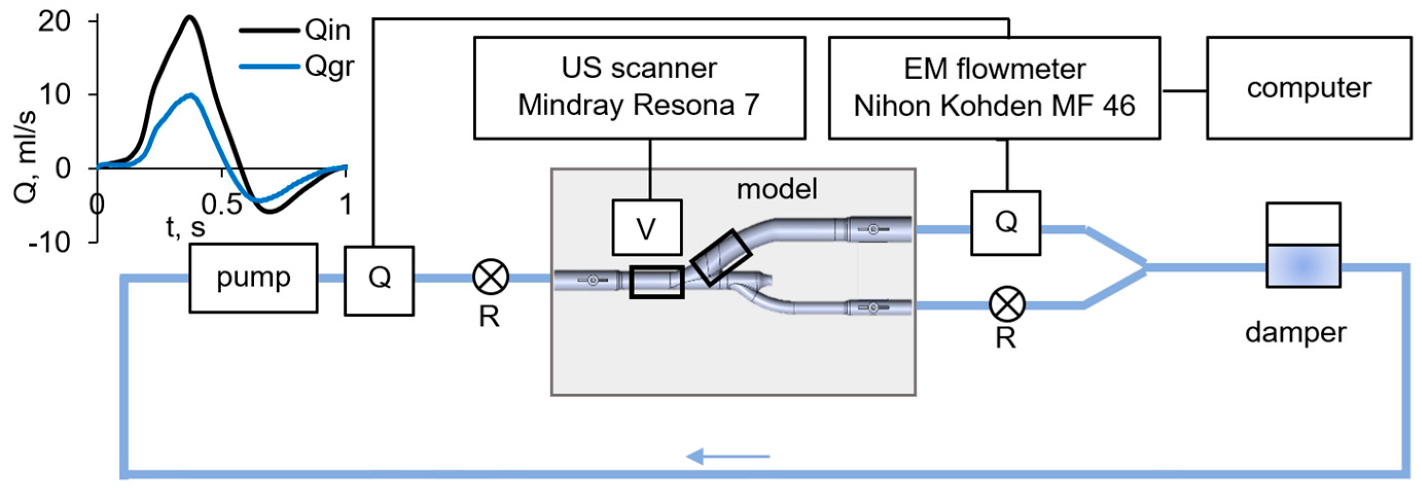
The measurement results presented in the present work were obtained using the V Flow vector visualization program implemented in the Mindray Resona 7 scanner (Shenzhen Mindray Bio-Medical Electronics Co., Ltd., Shenzhen, China). The V Flow technique is based on multi-directional Doppler US using an interleaved plane wave and focused wave transmissions [
16]. The blood flow structure after short-term scanning at high frame rates and short post-processing is presented in the form of a non-stationary 2D vector velocity field in the scanning window. The color and length of the vectors correspond to the magnitude of the velocity module. The results do not depend on the angle of installation of the transducer relative to the blood vessel. The video clip of pulsatile blood flow can be viewed by increasing the cycle duration by 7–200 times. The clinical testing of this program was carried out both by the developers of the method and by some scientific groups in different countries [
30,
33]. Using the V Flow method, vector blood flow velocity fields were studied in the carotid and femoral arteries [
34], arteriovenous fistulas [
35], and veins of the lower extremities [
36]. The authors of the report [
37] tested the V Flow method in a “reference” flow using two commercial blood flow phantoms. When using a string phantom, the error in measuring the axial velocity was evaluated as 3.8%, and in the case of the Doppler flow phantom, the error in measuring the bulk velocity was 5.2%.
The authors of the present work are not aware of any studies devoted to comparison of the measurement data by the V Flow method with the results of the numerical simulation of three-dimensional blood flow. The method was compared with other clinical measurement methods only based on the integral parameters of blood flow. The purpose of this work is a comparative study in vitro and in vivo of the pulsatile blood flow velocity field in the area of the graft branch from the femoral artery during femoral popliteal bypass surgery (proximal anastomosis) using two methods, which are the high-frame-rate ultrasound vector imaging of V Flow and the finite-volume numerical simulation technique for solving the Navier-Stokes equations.
3. Numerical Simulation Technique
3.1. Computational Domains and Grids
The numerical modeling of pulsatile blood flow in the area of the proximal anastomosis was carried out based on Navier–Stokes equations using the average model and a personalized one.
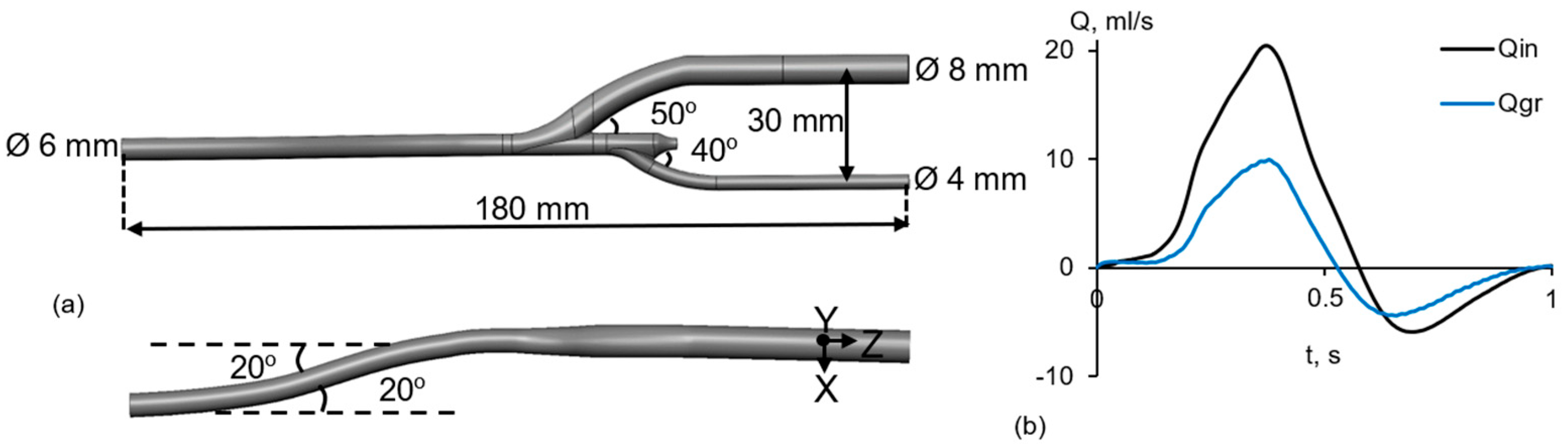
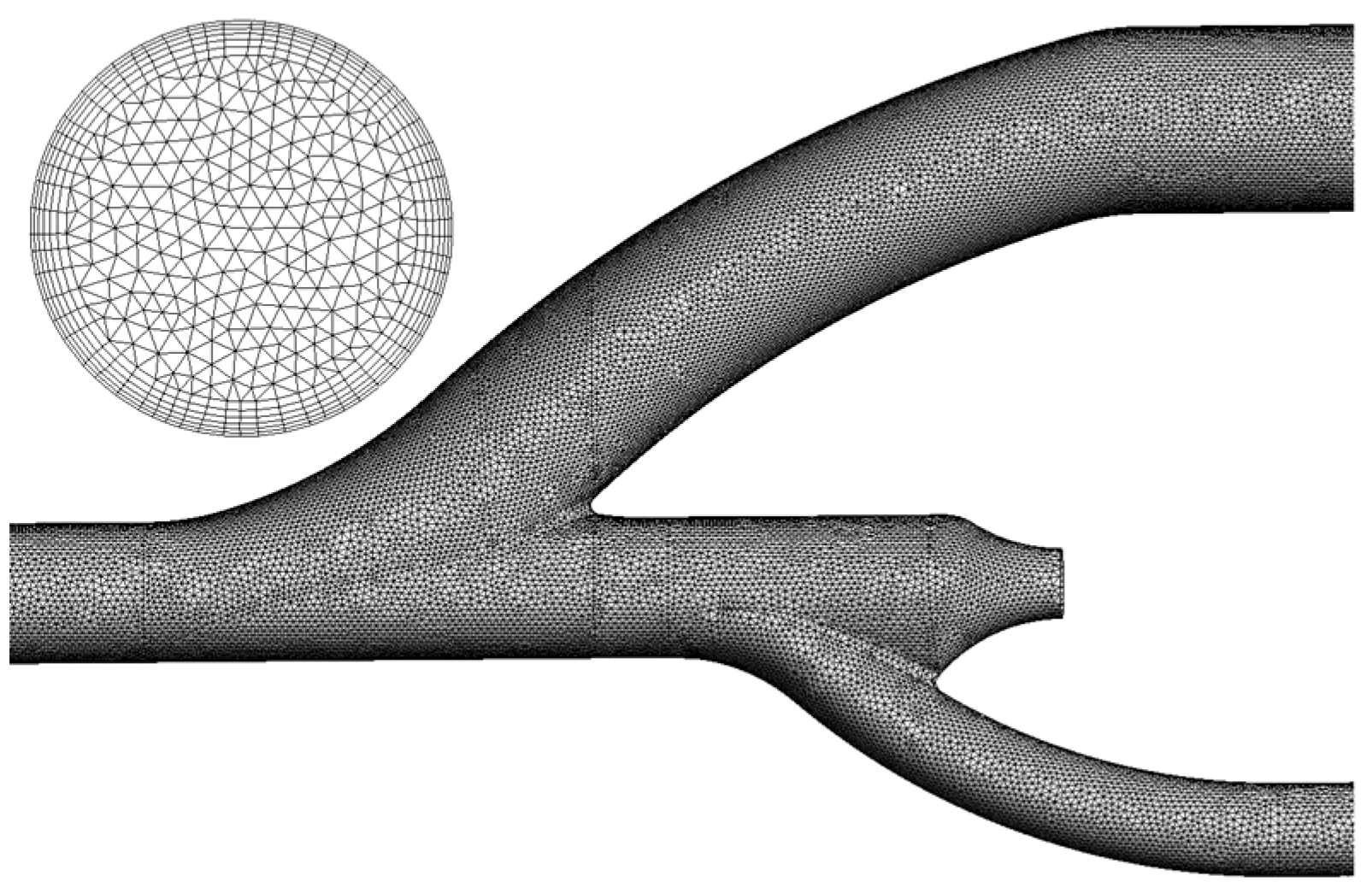
In the case of the average model, the used computational domain fully corresponded to the 3D geometry of the laboratory model of the described-above anastomosis area, with the addition of the supply tube. The calculation results shown in the present paper were obtained with a basic computational grid that included 3.2 million elements, mainly tetrahedra (
Figure 5). Near the wall, the grid contained prismatic layers for a better resolution of near-wall flow. The thickness of the elements closest to the wall was about one hundredth of the diameter of the vessel. At a preliminary stage of calculations aimed at the analysis of grid dependence, two more grids, characterized by decreased and increased characteristic sizes of the elements, were also constructed, maintaining a similar spatial distribution. The coarser and the refined grids contained 500 thousand and 11 million elements, respectively. Some results of the grid sensitivity analysis are presented in
Section 3.3.
Using the procedures described in our previous reports [
15,
16,
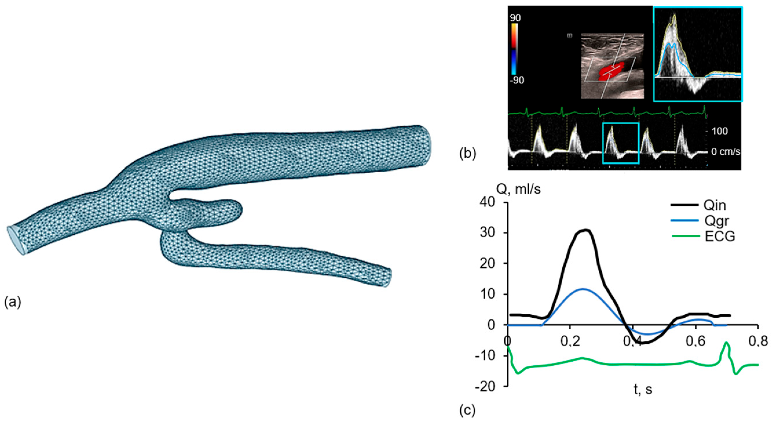
17], a personalized geometric model of the proximal anastomosis area of the patient, for whom an examination was carried out in the University clinic 7 months after the operation, was built based on data of MSCT angiography. This personalized model is illustrated in
Figure 6a. The diameter of the model section related to the common femoral artery (CFA) is evaluated as 7 mm, whereas the outlet diameter of the captured graft section is 9 mm. The computational grid generated for the personalized model consisted of 2 million elements.
3.2. Boundary Conditions
Changes in the average flow rate over time were specified as boundary conditions at the inlet to the computational domain corresponding to the CFA, section S
in, and at one of the outlets corresponding to the graft, section S
gr. For the anastomosis average model, the temporal changes of the flow rates at sections S
in and S
gr were defined by the measurements performed on the experimental setup (
Figure 1b). In the case of the personalized model, the flow rate curves Q
in(t) and Q
gr(t) shown in
Figure 6b were obtained via processing the results of ultrasonic Doppler measurements at a section of the CFA and at a distal section of the graft. The ratio of the maximum flow in the graft to the maximum inlet flow was equal to 0.38. Data synchronization for the CFA and the graft sections was provided by the electrocardiogram signal. The patient had a biphasic blood flow rate curve measured in CFA. The duration of the systolic phase was 0.23 s with a peak velocity of 81 cm/s, the duration of the reverse flow was 0.14 s with the peak velocity of 16 cm/s, the cycle duration was 0.7 s, and the constant diastolic velocity—8 cm/s (
Figure 6c).
The inlet velocity distribution was assumed to be uniform over the vessel cross-section. At the second outlet, the reduced pressure was set to zero. The no-slip condition was specified on all walls and treated as rigid. The measured radial displacements of the vessel wall were quite low: 0.05·DCFA for CFA and 0.005·Dg for the graft.
3.3. Computational Aspects
For the simulations, the dynamic viscosity of the blood-mimicking fluid was assumed to be 0.0035 Pa·s, and the density was 1050 kg/m3. With these properties of the fluid, the characteristic Reynolds number, based on the inlet flow rate at the maximum flow instant and on the diameter of the inlet section, is evaluated as 1390 for the anastomosis average model and 1640 for the personalized one.
The mean Reynolds numbers, evaluated with the time-averaged inlet velocity over the forward-flow phase, are about 500 for both models. It means that the flow regime is very far from regimes of developed turbulence, and one would expect only local (in space and time) manifestations of incipient turbulence. There are no known statistical turbulence models in the literature that could be applied to reliably capture the smoothing impact of this local incipient turbulence on the major large-scale components of the flow developing in the vessel models. The application of advanced approaches aimed at the resolution of a broad spectrum of vortices in the flow (direct numerical simulation or well-resolving large eddy simulation) is out of the scope of the present study. Apart from the need for enormous computational resources, the use of these approaches would require well-defined information about the spectrum of inlet disturbances, which is very problematic to extract from experiments.
Taking into account the above-mentioned circumstances, the present numerical simulation was carried out under the assumption that the flow is quasi-laminar. With this assumption, the physical smoothing action of small-scale eddies in potential areas with local turbulence is replaced by the dissipative properties of the numerical scheme used for solving the discretized Navies–Stokes equations.
Calculations of pulsatile flow fields for both the anastomosis average model and the personalized one were performed using the commercial finite-volume CFD package Ansys CFX 18.2 (Ansys Inc., Canonsburg, PA, USA). The “High Resolution” scheme was activated for the calculation of the convective fluxes, being, in fact, the second-order accuracy upwind scheme introducing a proper dissipation. The second-order backward Euler scheme was used for physical time stepping. The final calculations were performed with time step equal to 0.01 s. The convergence criterion was the reduction of normalized residuals to 10−6 at each time step. Typically, the calculations were carried out for three cycles, starting with the conditions corresponding to an initially quiescent fluid. It was established that the calculated flow fields in the second and third cycles practically coincided.
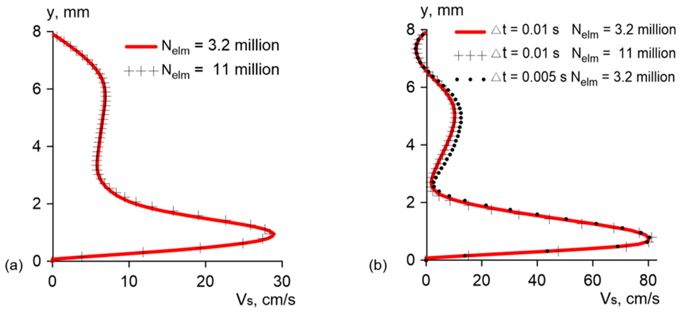
Figure 7 presents some results of the grid and time-step sensitivity analysis performed to assess the appropriateness of the basic computational grid characteristics, as well as the chosen time step of 0.01 s. This analysis included two series of computations dealing with the anastomosis average model. The first one covered a comparison of the steady-state solutions obtained with the basic and refined grids (N
elm = 3.2 and 11 million) for the inlet Reynolds number equal to 480, which is just the mean Reynolds number evaluated with the time-averaged inlet velocity over the forward-flow phase. A well agreement of the flow fields computed with two grids is illustrated by
Figure 7a, where the streamwise velocity profiles related to the graft model are compared. The second series of the grid sensitivity analysis covered a comparison of the pulsatile flow solutions computed with two grids and different time steps for the time-dependent boundary conditions, as described in
Section 3.2. Particular results of this comparison are demonstrated in
Figure 7b, where three velocity profiles, also taken in the graft area, are shown for the maximum flow instant. The performed analysis of the numerical solution sensitivity to changes in the grid size and time step allowed us to conclude that the basic grid and the chosen time step were quite acceptable for simulation in the case of the anastomosis average model. The structure and size of the base grid elements for the personalized model were chosen similarly to the average model case.
4. Results and Discussion
To compare the experimental and computational results obtained for the average model of the proximal anastomosis two characteristic instants were chosen, the first of which corresponds to the maximum forward flow rate; the second corresponds to the maximum reverse flow rate.
Figure 8 and
Figure 9 present a comparison of CFD and V Flow data for the scanning window positioned before the model graft branch (
Figure 3), whereas
Figure 10 and
Figure 11 cover the compared data obtained with the window positioned in the model graft, just after the branching (
Figure 3).
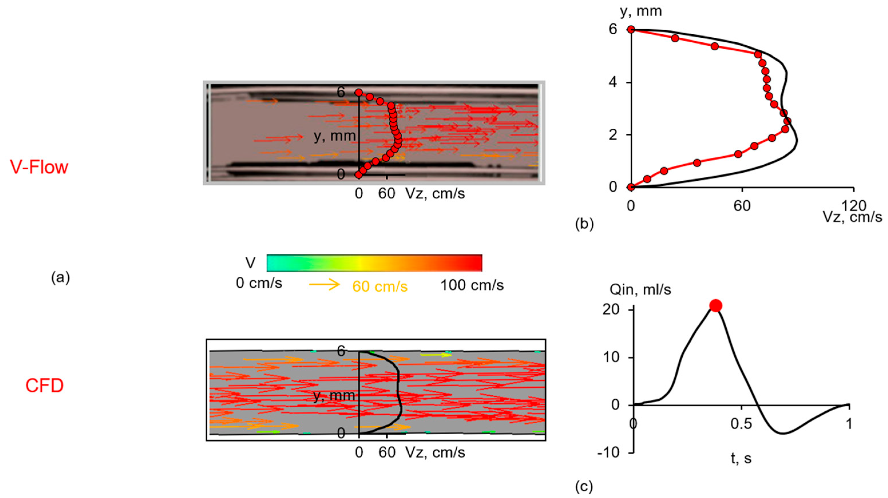
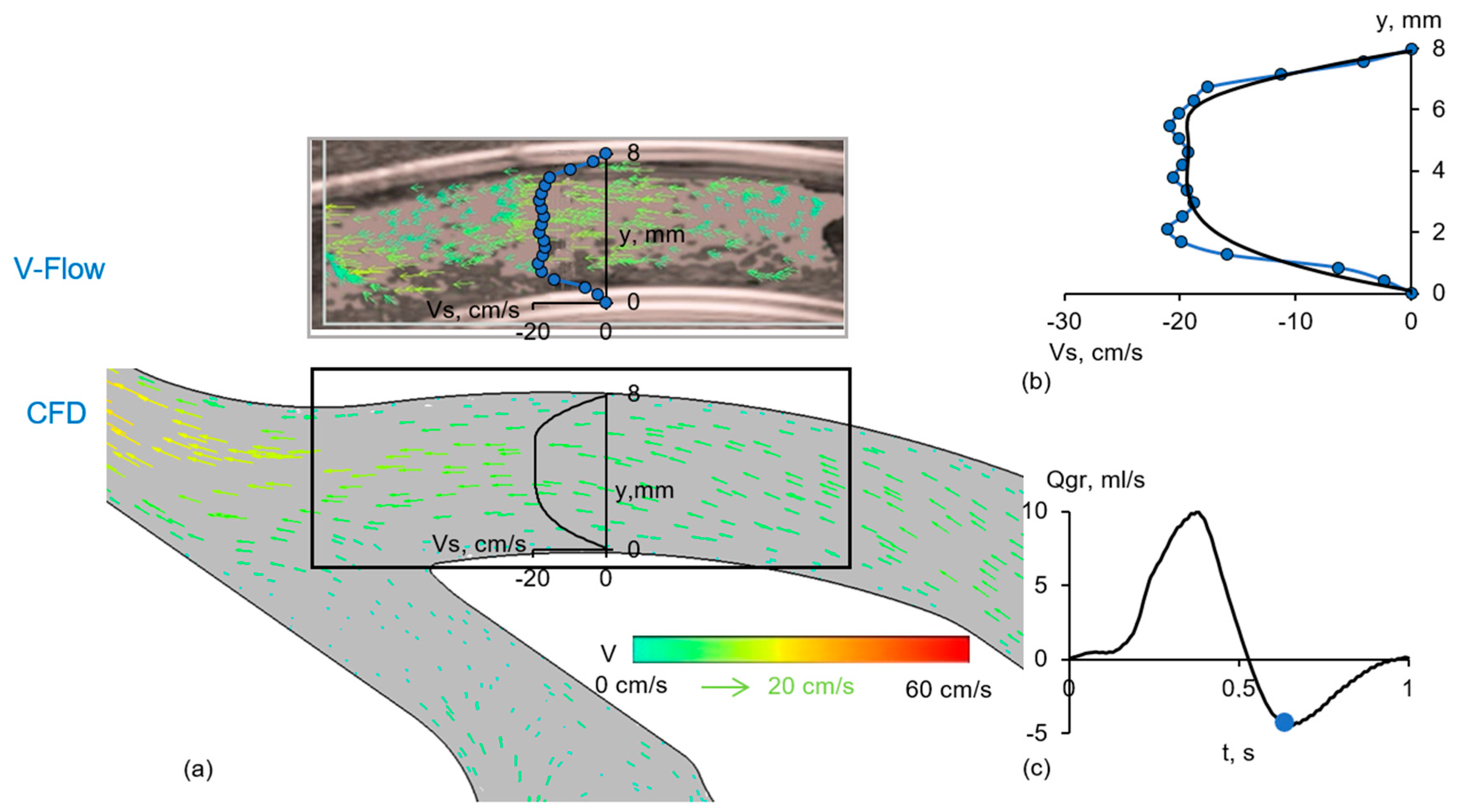
For the section covered by the first window, both the V Flow technique and the simulation visualized the velocity field with nearly straight streamlines parallel to the vessel wall, even for the chosen instant of the reverse flow (
Figure 8a and
Figure 9a). The measured and calculated profiles shape of the streamwise velocity, V
s, are in reasonable agreement (
Figure 8b and
Figure 9b, V
s = V
z in this case). The difference between the measured and calculated maximum velocity does not exceed 8%. The standard deviation of the experimental velocity profile points from the calculated one was 9% for the forward flow profile (
Figure 8) and 1% for the reverse flow profile (
Figure 9), with respect to the peak bulk velocity in the section where the velocity profile was measured.
Note that the experimental profiles were constructed by averaging the data obtained in five independent experiments to reduce the influence of random experimental errors.
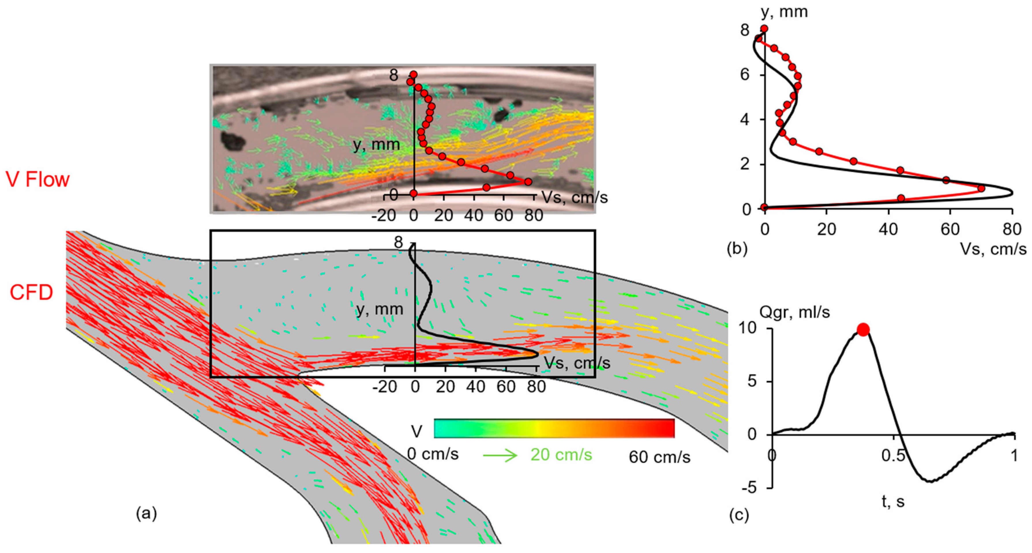
The velocity vector patterns obtained by the two methods for the maximum flow rate instant in the case of the scanning window positioned in the graft are compared in
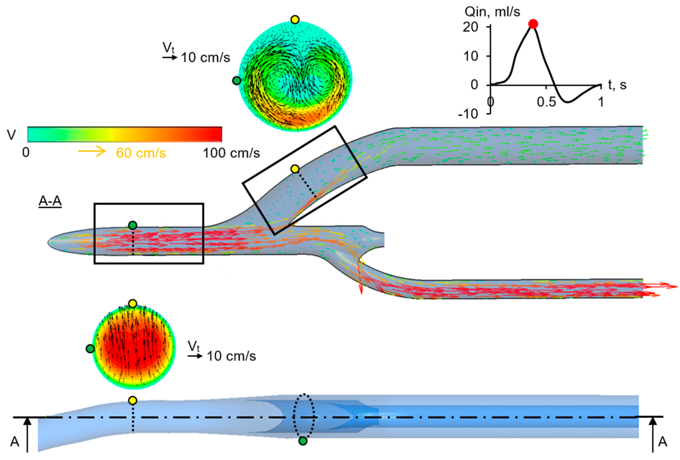
Figure 10a. Both the experimental observations and the simulation show the formation of a large recirculation zone with relatively low velocities. The CFD pattern covering a larger area compared with the V Flow scanning window (see also
Figure 3) shows that this recirculation zone, adjacent to the external side of the graft, originates at the beginning of the vessel bifurcation. On the internal side of the graft, the flow is a high-velocity jet. The profile shapes of the measured and calculated streamwise velocity, Vs, shown in
Figure 10b, are in an acceptable agreement. The difference between the measured and calculated maximum values does not exceed 12%. The standard deviation of the experimental velocity profile points from the calculated ones was 13% for the forward flow profile (
Figure 10) and 3% for the reverse flow profile (
Figure 11), again with respect to the peak bulk velocity in the section where the velocity profile was measured.
The post-processing of the CFD solution allows one to better understand the flow structure in the graft, which is essentially three-dimensional for the forward flow phase. The latter is illustrated in
Figure 3, which also covers a cross-flow vector pattern superimposed on the streamwise velocity map for a graft cross-section. One can observe that the secondary flow in the graft section under examination has the form of a vortex pair.
Figure 11 presents a comparison of CFD and V Flow data obtained for the examined part of the anastomosis average model at the instant of maximum reverse-flow rate. One can observe that, in this case, a relatively simple flow structure with a unidirectional fluid motion is formed both in the graft and in the femoral artery part. The velocity vector patterns obtained with the two methods are quite similar, and the measured and computed profiles of the streamwise velocity in the graft section are in reasonable agreement.
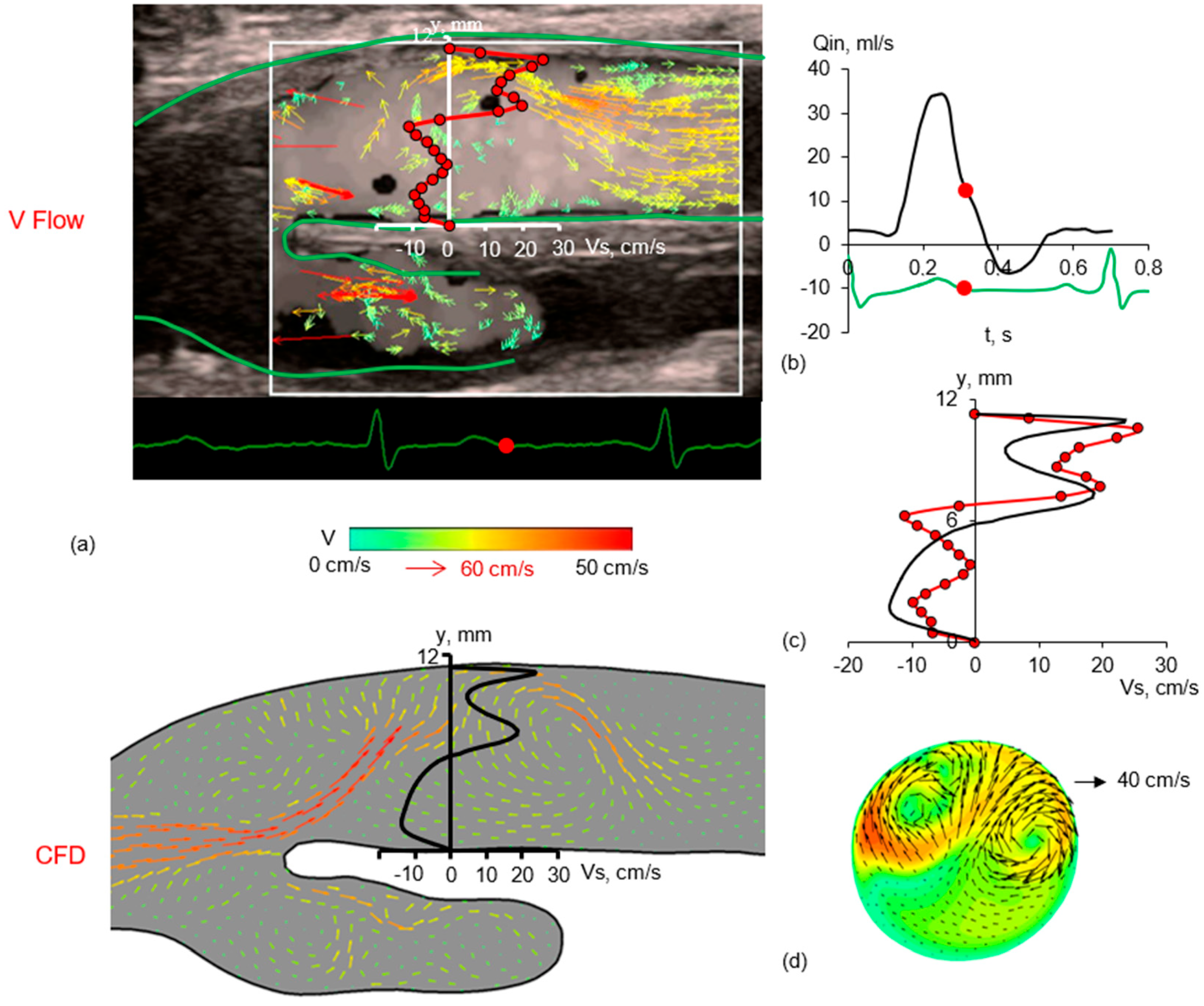
In
Figure 12, the results of clinical measurements performed by the V Flow method for the graft branch from the femoral artery are compared with the results of the numerical simulation for the personalized model. In this case, a time instant corresponding to the phase of decreasing the forward flow (marked in
Figure 12b) was chosen for comparison.
One can state the similarity between the flow patterns, which were recorded in vivo and generated by the calculations using the personalized computational model. It should be emphasized that for the chosen instant, the flow structure in the scanning window is especially complicated and characterized by the presence of multiple vortices and an intensive cross flow directed from the inner wall of the graft to the external one (
Figure 12a). It is also remarkable that the instant cross-flow pattern predicted by CFD for the chosen section (
Figure 12d) looks like a vortex pair, but the direction of its circulation is opposite compared to that illustrated for the instant of the maximum flow in the anastomosis average model (
Figure 3). Our experience in the parametric numerical simulation of pulsatile blood flow in different proximal anastomosis models, presented partially in [
15,
16,
17], allows us to conclude that the circulation direction in the formed vortex pair depends not only on the examined phase of the cycle but also on the graft-to-CFA flow rate ratio and the individual geometry. The profiles of the streamwise velocity, V
s, measured and calculated for a graft section, are shown in
Figure 12c (here, the experimental profile is a result of phase-averaging over five cycles of blood flow recorded in vivo). The difference between the measured and calculated maximum velocity of forward and reverse flow does not exceed 15%. The standard deviation of the experimental velocity profile points from the calculated one was 13% (
Figure 12), with respect to the peak bulk velocity in the section where the velocity profile was measured.
In general, the plots presented in
Figure 12 indicate that the results of the clinical V Flow measurements and the CFD simulation are in reasonable agreement. It should be noted here that due to a number of uncertainties, both arising when constructing a personalized computational model and inherent in the V Flow method itself, one can hardly expect complete consistency in the results obtained using the two methods. General limitations of the used methods/approaches can be summarized as follows. The V Flow method has the following limitations: (i) the impossibility of obtaining data for 3D vector flow visualization, (ii) the size of the scanning window is 20 × 27 mm only, (iii) the depth of the scanning window is limited by 50 mm, and (iv) recording time is limited by 3 s. The limitations of the applied numerical simulation technique are (i) neglecting pulsations of the vessel walls, and (ii) the assumption of the quasi-laminar flow regime. The main difficulty when comparing the results obtained with the two methods is attributed to the choice of a longitudinal section of the personalized model with the calculated 2D vector velocity pattern that would be as close as possible to the position of the scanning plane during the clinical study.
5. Conclusions
The V Flow high frame rate ultrasound vector flow imaging method and a CFD technique have been used for a coordinated study of the pulsatile velocity fields in the area of the proximal anastomosis for femoral popliteal bypass surgery in vitro and in vivo. Obtained by two methods, the dynamic vector images of the velocity field and constructed streamwise velocity profiles in the scanning plane of the flow in the area of the graft branch are in reasonable agreement, both in the case of the anastomosis average model developed for laboratory studies and in the case of the personalized model constructed to compare with clinic measurements.
Although the flow at the site of the graft branch from the artery depends significantly on the individual geometry, some general patterns can still be noted. At the beginning of the acceleration phase of the forward flow, as well as during the reverse flow phase, the fluid motion in the graft is unidirectional. In the accelerated forward flow, a separation zone appears at the external wall of the graft, rapidly increasing in size, with a significantly three-dimensional flow character and the determining role of the developed cross flow. During the deceleration phase of the forward flow, a relatively narrow zone of high flow velocities, initially adjacent to the internal wall of the graft, moves away from the wall, resulting in the formation of a large zone occupied by several vortex structures with opposite circulation.
The attractive advantages of the applied ultrasound high frame rate vector imaging technique are (i) the ability to carry out measurements of blood flow in real vessels, (ii) a high rate of obtaining a large volume of recorded data on pulsatile blood flow in complex areas of the vascular bed, and (iii) the possibility of the subsequent repeated slow-motion viewing for the purpose of processing and analysis of the received data. At the same time, the ultrasonic vector flow visualization method provides very limited opportunities for identifying three-dimensional vortex formations in the area under study, which, on the contrary, is fully provided by up-to-date CFD technologies; however, they are for flow in the models of real vessels only.
The complementary use of the V Flow method and three-dimensional numerical simulation has great potential for an in-depth study of the dynamics of pulsatile blood flow in branching sections of the vascular bed.

 ,
, 


