
Impact of Crustacean Morphology on Metachronal Propulsion: A Numerical Study

1
Pioneer Academics, 30 S 15th St, 15th Floor, Philadelphia, PA 19102, USA
2
Department of Civil & Environmental Engineering, Duke University, Durham, NC 27708, USA
*
Author to whom correspondence should be addressed.
Fluids 2024, 9(1), 2; https://doi.org/10.3390/fluids9010002
Submission received: 3 November 2023
/
Revised: 27 November 2023
/
Accepted: 21 December 2023
/
Published: 23 December 2023
(This article belongs to the Topic Computational Fluid Dynamics (CFD) and Its Applications)
Abstract
:Metachrony is defined as coordinated asynchronous movement throughout multiple appendages, such as the cilia of cells and swimmerets of crustaceans. Used by species of crustaceans and microscopic cells to move through fluid, the process of metachronal propulsion was investigated. A rigid crustacean model with paddles moving in symmetric strokes was created to simulate metachronal movement. Coupled with the surrounding fluid domain, the immersed boundary method was employed to analyze the fluid–structure interactions. To explore the effect of a nonlinear morphology on the efficiency of metachronal propulsion, a range of crustacean body shapes was generated and simulated, from upward curves to downward curves. The highest propulsion velocity was found to be achieved when the crustacean model morphology was a downward curve, specifically a parabola of leading coefficient k = −0.4. This curved morphology resulted in a 4.5% higher velocity when compared to the linear model. As k deviated from −0.4, the propulsion velocity decreased with increasing magnitude, forming a concave downward trend. The impact of body shape on propulsion velocity is shown by how the optimal velocity with k = −0.4 is 71.5% larger than the velocity at k = 1. Overall, this study suggests that morphology has a significant impact on metachronal propulsion.
1. Introduction
Animals have developed diverse methods of moving in aquatic environments. Most species of fish undulate varying parts of their bodies to create thrust and swim. The locomotion of fish is often further propelled or controlled by median fins [1]. Jet propulsion is another such approach to movement, used by cephalopods like octopuses and jellyfish. In this process, animals forcefully eject a jet of water to propel themselves in the opposite direction [2]. Microscopic ciliates use densely packed arrays of cilia to propel themselves, while crustaceans use pleopods, or swimmerets, to swim forward. Curiously, cilia and pleopods both move in a metachronal rhythm [3,4].
In biology, metachronal motion describes asynchronous, yet coordinated movement of multiple similar appendages. These motions are asynchronous because they are performed at different times, one after another in a cyclic pattern. Research has suggested that synchronous oscillation produces no propulsion, while metachronal oscillation enables forward movement, achieving the act of swimming [5]. Further, asynchronous appendage motion results in superior performance over synchronous movement in both efficiency and velocity [6,7,8].
Metachronal propulsion can be classified into symplectic and antiplectic types. Also described as head-to-tail, symplectic metachrony occurs when the first appendage begins its movement, followed by the remaining ‘arms’ in sequence. Antiplectic metachrony, or tail-to-head, starts with the last appendage and propagates forward. Symplectic and antiplectic metachrony have inverse effects on motion; antiplectic movement causes an increase in the net flow of surrounding fluid, while symplectic movement leads to a decrease [9].
Thus, a significant factor that affects the behavior of metachronal propulsion is the phase difference, which is the lag between the motions of adjacent legs [10]. In this study, we attribute antiplectic metachrony with a positive phase difference and symplectic metachrony with a negative phase difference.
1.1. Metachronal Propulsion in Crustaceans
Crustaceans use metachrony in their swimmerets, which are small appendages used for swimming [11]. Swimmeret motion can be divided into the power stroke (PS) and the return/recovery stroke (RS), where the PS propels the crustacean forward and the RS returns the appendage to the appropriate position [12]. There are generally four to five rows consisting of a pair of swimmerets; each pair of swimmerets beats synchronously, but each row is asynchronous [13].
A qualitative justification behind the use of metachronal propulsion in crustaceans is that the minuscule lengths between their swimmerets are prone to causing interference in synchronous movement [14]. Therefore, applying a phase shift on swimmeret cycles can help mitigate inefficiency or produce beneficial effects [15].
Using a drag-based mechanic model, metachronal motion in the swimmerets has been shown to increase body velocity, leading to the result that metachrony produces a velocity about 10% greater than synchronous movement [16]. However, the drag-based model fails to consider fluid–structure effects, which turn out to significantly impact propulsion.
Iterating over this flaw, the immersed boundary method was used to simulate models of crustaceans varying in paddle number over a range of phase differences and Reynolds numbers from 0 to 100 [13]. In this range, the researchers discovered that the average flux over these Reynolds numbers follows the same trend from a phase difference of −0.2 to 0.2, varying more as the phase difference approaches the endpoints of −0.5 and 0.5. By testing different numbers of paddles sharing the same spacing as before, researchers [13] found that the correlation between efficiency and the number of paddles reversed as the Re was increased from 0.1 to 100. However, the model with four paddles was 85–90% efficient over the range, showing that possessing four paddles is a reasonable assumption for the low Reynolds number used in this study.
1.2. Impact of Body Structure on Propulsion
Since the rigid crustacean body is attached to its appendages, this boundary has a significant effect on the fluid flow from metachronal propulsion. Depending on the shape, the body structure can either limit or promote fluid movement, directly correlated with the effectiveness of crustacean locomotion. Additionally, this study allows crucial insight into the evolutionary motivations for a crustacean’s morphology, opening up discussions of optimality. For these reasons, exploring the effect of body shapes on metachronal propulsion is significant.
Following previous research, we modeled the crustacean’s power and return stroke as symmetric identical movements [13]. The return stroke features additional drag asymmetry due to a changing paddle size, which has been previously modeled with porous paddles [15]. This simplification was made to isolate the mechanics of metachronal propulsion’s improved efficiency over other propulsion methods, rather than convolute the experiment with an additional source of forward movement.
1.3. Methods of Investigating Metachronal Propulsion
Previously, researchers have used many methods to analyze the mechanics of metachronal propulsion through videos, robotic models, and fluid simulations. Video analysis explores metachrony through biological observations, while modeling via robot or software aims to simulate metachronal motion.
1.3.1. Video Analysis
Videos of metachronal locomotion can be analyzed frame-by-frame, noting the movement of the organism’s legs as the video progresses [6,14,17]. Particle image velocimetry can be used in tandem to acquire information on the organism’s kinematics [18]. This method is most convenient if the studied organism is commonly available and visible to the human eye.
1.3.2. Robotic Modeling
Another method of examining metachrony is through robotic implementations, in which a mechanical setup is used to mimic a biological equivalent. For example, magnetically actuated ciliary arrays can be used to simulate the cilia in cells [8,19]. Through this method, it has been discovered that antiplectic metachronal motion in cilia leads to an increased net flow and the formation of vortices [9,20]. Another application of robotics can be seen with a robotic crustacean model [4,21,22]. In the aspect of isolating a mechanism’s effect, robotic modeling proves advantageous over video analysis.
1.3.3. Fluid Simulations
Computational fluid dynamics (CFD) can be employed without biological samples or mechanical equipment, making it an accessible method of simulation and analysis. CFD includes a wide variety of applications, such as observing factors like temperature, velocity, pressure, and drag in a design [23,24,25,26]. Applying CFD to metachronal motion in cilia shows that it is beneficial, leading to the increased size range of accessible food particles, optimized mucus transport, and optimized flow [27,28,29].
One facet of CFD relevant to metachronal propulsion is simulating fluid–structure interactions, which directly address how structures performing metachronal propulsion shape surrounding flows. Like robotic modeling, CFD simulations can exclude the impact of unwanted factors. A particular framework, the immersed boundary method, has been prevalent in modeling fluid–structure interactions by using Lagrangian points to model the structure and Eulerian coordinates to represent the surrounding fluid [30].
1.4. Goals
Although [13,21,22] explored the effects of the phase difference, number, and length-to-spacing ratio in appendages, their analyses were conducted under the simplifying assumption of a linear morphology. For the first time, we ran and assessed simulations to examine the effect of a nonlinear morphology on metachronal propulsion.
2. Methods
The 2-dimensional crustacean model consists of four mobile paddles below a curved wall, representing the swimmerets and the body, respectively. Mirroring a crustacean’s biology, both of these structures were modeled as rigid boundaries immersed in a fluid.
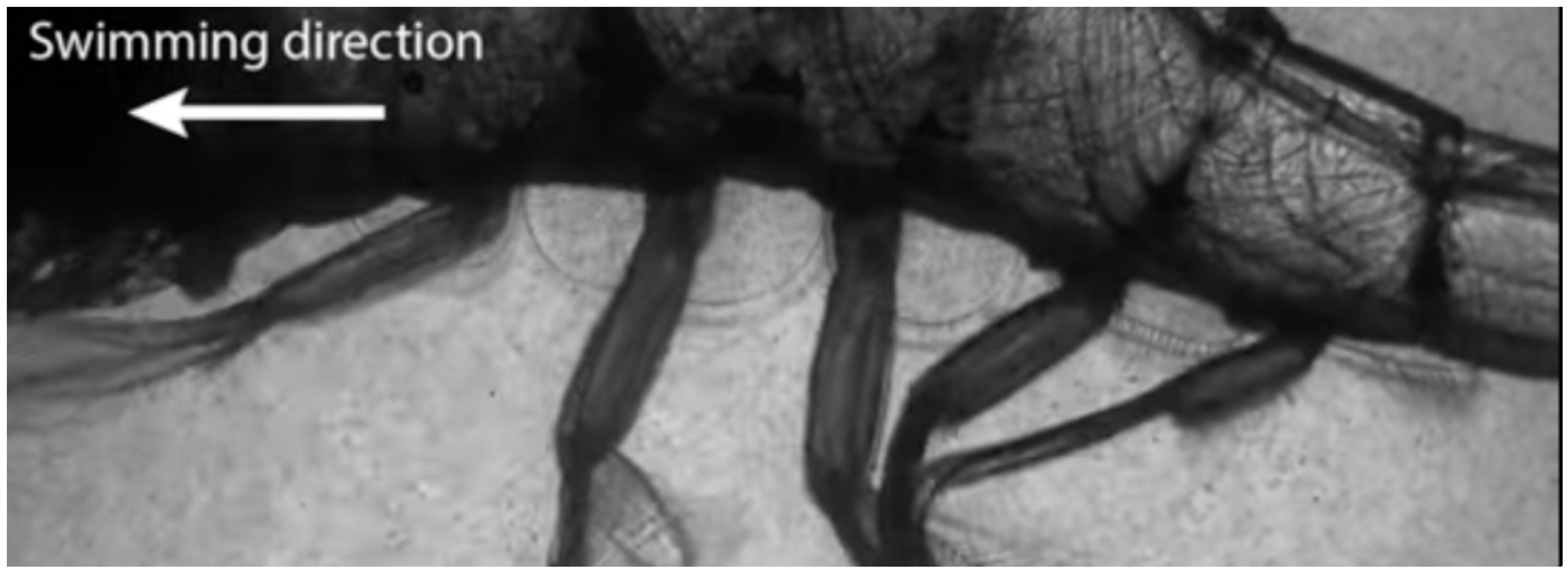
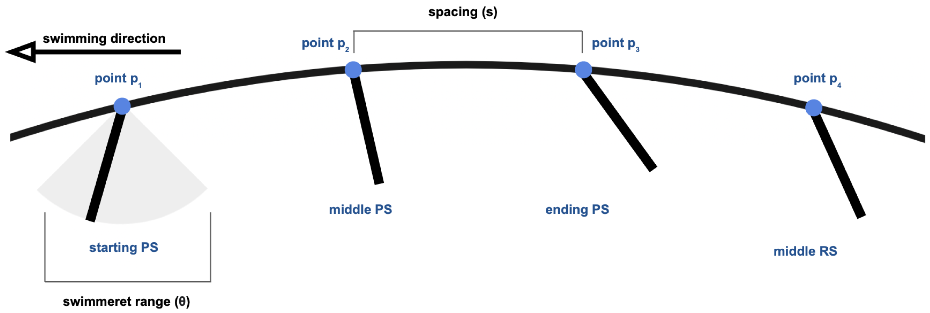
The curved body of the model was designed to recreate biological equivalents. In Figure 1, a common American prawn demonstrates an arched anatomy during metachronal locomotion. In Figure 2, many key aspects of the crustacean model are displayed, as well as an example of antiplectic metachronal propulsion. While the rightmost paddle is executing the return stroke, the others are still finishing power strokes in sequence.
For our use of a flow with a low Reynolds number, where the inertial forces are less significant, we decided to use four paddles to perform our study [31]. Research has also been performed on the effect of appendage spacing on metachronal propulsion, but for the purposes of isolating one change, the fluid simulation for our research assumes a constant, common spacing length of 0.2 m [21].
While crustaceans feature multiple joints that assist the power and return stroke, the paddles in this study were modeled as single joints to observe the isolated effect of metachronal motion. Both mechanisms aid the crustacean in achieving propulsion, but we chose to primarily examine metachronal motion and, therefore, simplified the movement into a singular paddle without joints. To avoid collisions between adjacent paddles, we modeled the paddle length to be 0.1
2.1. Paddle Movement
The paddles are indexed i = 1, 2, 3 and 4 from left to right, attached to the body at points , with coordinate pair . In the swimmer’s Lagrangian structure, joined endpoints with a stiffness constant form the paddle structure. Let denote the jth point in paddle i, with x-coordinate and y-coordinate . Then, the movement of point can be modeled by the original parametric equations:
where and describe the starting and ending positions of the paddle in radians. For our model, and , shown in Figure 1 by the gray range around the first paddle. These values were chosen to best provide a general stroke range for crustaceans, comparable to the values used in prior studies [13]. r represents the radius of motion, obtained by using the distance formula between and . T represents the combined period of the power and return stroke, and the two cases in the expression symbolize the PS and RS, respectively. the phase difference between adjacent paddles in seconds, is incorporated in the expression through t. Representing the current time in period T, t is formulated with the following original equation.
Here, represents the time since the start of the simulation, where t can be conceptualized as denoting the current progression through . It is worth noting that this formulation describes tail-to-head motion; paddle 4 does not experience any phase shift, and the leftmost paddles are shifted the most. Altogether, the parametric expression describes a circular motion around a circle with center , creating a periodic oscillation between angles and . This forms the power stroke and return stroke patterns.
2.2. Crustacean Morphology
To mimic the natural arch of a crustacean during metachronal propulsion, we used a parabolic formula to describe its body shape. The parabolic body’s vertex is halfway between paddles 2 and 3, providing a symmetric curve over the four paddles. Such points on the body are described by the equation:
where 0.5 describes the x-coordinate of the vertex and 0.3 describes the body’s highest or lowest point. This formulation ensures that, for , the full range of motion for all paddles is contained in the fluid domain. In the fluid simulation, this parabolic morphology is represented by short line segments that collectively approximate the parabola.
2.3. Model Configuration
For this model, the horizontal spacing s between paddles is held at a constant of 0.2 m, and each paddle is 0.1 m long. The main motivation behind this choice is that it allows the paddles ample room to create flow, yet still promotes fluid interaction. A fixed horizontal spacing allows for increased ease of coordinate formulation, so that is simply 0.2i. The parameter follows the parabolic equation of the curved body. The domain of the immersed boundary solver is 3 m wide and 0.6 m tall, capturing the crustacean model and fluid behind it.
Period T was set to 0.05 s, so the symmetric PS and RS both took 0.025 s to execute. The value of T does not affect any results as long as the total simulation time is adjusted to include five full periods for every paddle. We considered the range to examine the optimal phase difference for our crustacean model and, then, set to a constant to consider the effect of body shape on propulsion. We chose not to examine , as research indicates that symplectic motion leads to decreased net flow [9]. Also, we did not simulate to create a comparison with the precedents set by [9,13].
A constant of 10 points makes up an outline of the crustacean’s body. Both the paddles and the body were assigned stiffness values of , where stiffness k describes the ratio of the applied force to the resulting displacement. A similar study of jellyfish propulsion [32] used a stiffness of to represent the deformable jellyfish bell. With a stiffness constant 2 orders of magnitude above , the deformation of the legs becomes negligible. The stability of the legs is demonstrated in the Supplementary Materials, where the limbs are not impacted by the surrounding flows.
2.4. Fluid Theory
Aside from the crustacean model, the behavior of the surrounding incompressible fluid is governed by the Navier–Stokes and continuity equations.
where , is the dynamic viscosity, is the fluid density, and F is the force exerted on the fluid by the paddles. Overall, the first equation states that the momentum’s rate of change is equal to the sum of the pressure gradient, viscous forces, and external forces exerted by the paddles. The second equation describes conservation of mass. The gravity term in the standard Navier–Stokes equation was neglected because, for simplicity, the motion is assumed to be horizontal.
The Reynolds number () of a fluid is significant in determining the flow regime. A smaller Reynolds number describes a flow where viscous effects dominate the behavior, and a higher Reynolds number implies that inertial effects preside instead. This dimensionless quantity can be calculated using the formula:
where c is the characteristic velocity and is the characteristic length. Setting c to the maximum speed of the paddle tip and to the paddle length results in . This low Reynolds number was chosen to focus on the effects of metachronal propulsion rather than increasing the resulting vorticity.
2.5. Immersed Boundary Software
In this study, we utilized the immersed boundary method for analyzing metachronal propulsion in crustaceans for the reason of improved universality over video analysis and the ease of robotic modeling. Furthermore, the ability to accurately model fluid–structure interactions is paramount for capturing the optimal configurations for metachrony.
While 3-dimensional models are possible, this study used 2-dimensional models for the purpose of simulation. We modeled the side view of a crustacean, capturing a cross-section where the body and appendages are visible. While 3D models can encapsulate more-realistic details of the crustacean, a 2D model preserves forward locomotion, the most-significant aspect, while reducing computation time exponentially. Using a 2D model has many precedents in effectively studying metachronal propulsion, from both simulating cilia and crustaceans [13,28].
The immersed boundary method was performed via IB2d, a software specifically developed for simulating 2-dimensional fluid–structure interactions. The IB2d software offers both a MATLAB and a Python implementation of the solver, including mesh generation and useful structures like springs, beams, targets, and more [33,34,35]. In our study, target points were extensively used to model the prescribed motion of the paddles. We chose IB2d over other CFD tools like IBAMR and Ansys due to the ease of installation and usage. IB2d is similar to another software, IBAMR, in performance and method, but the former’s installation requires no additional downloading of other libraries. While the Ansys Suite allows for fluid–structure interaction through system coupling and motion through user-defined functions (UDFs), the required setup is much more complex. Also, IB2d allows for more flexibility than commercial software by being open source, allowing for user edits. A specific feature of IB2d is that it does not require external driving forces to model fluid–structure interactions, isolating the effects of propulsion [33]. This software has precedents of successful use in multiple studies involving fluid dynamics and solid–fluid interactions [32,36].
2.6. Immersed Boundary Configuration
The domain that we are solving over consists of decoupled Eulerian coordinates and Lagrangian points, essential for the immersed boundary method. The 100 by 20 Eulerian grid defines the fluid domain, where the Navier–Stokes equations take effect. Lagrangian points outline the crustacean model, with 3 points marking the endpoints of each leg and 10 points describing the body. At each time step, the motion of the paddles is translated into forces, which are then interpolated to affect the fluid flow. This occurs every 10 μs for 0.25 s. This ensures that the last paddle experiences five full periods of motion, but since the other paddles start in the middle of a stroke, they will not necessarily undergo five full periods even though they move at the same speed as the last paddle.
2.7. Performance Metrics
To analyze the performance of metachronal propulsion, we averaged the horizontal velocity across all Eulerian points and times. For every time step, we iterated through the 100 by 20 Eulerian grid and averaged the horizontal velocity at every point. Then, we took the average of this average horizontal velocity over all time steps from 0 s to 0.25 s. Since the model aims to swim forward or right-to-left, as shown in Figure 3, a positive velocity represents forward metachronal propulsion.
2.8. Convergence Analysis
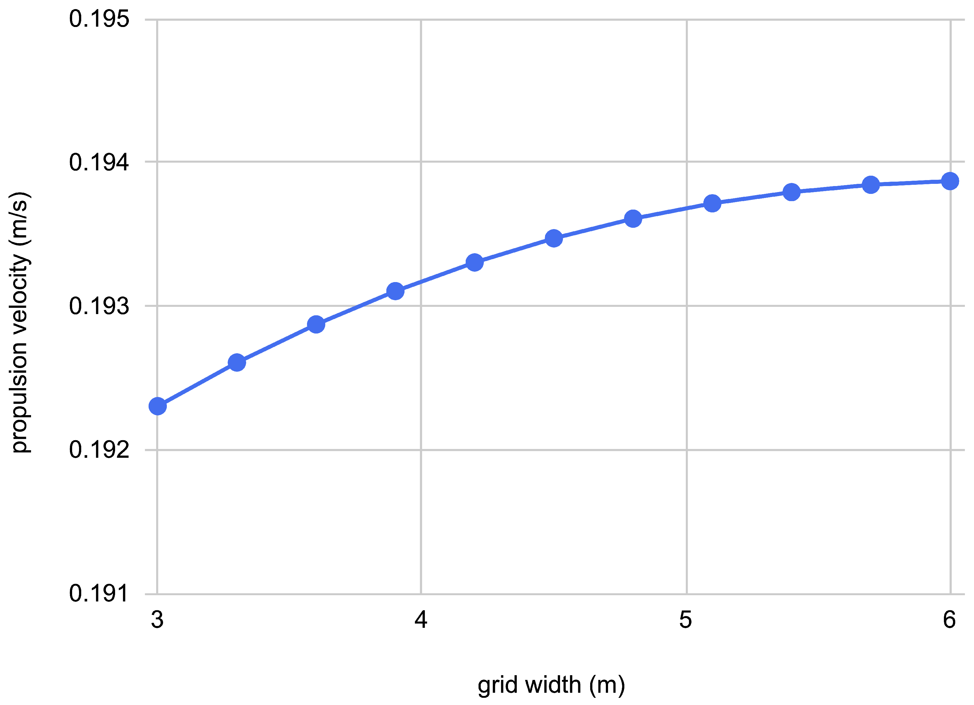
We performed a spatial grid convergence test to determine how the computational domain’s size affected the results. To isolate the width, we preserved the grid spacing and height of the Eulerian grid. We investigated the case where , with a computational domain of height m and a varying width . To ensure that Eulerian points are equally spaced in the domain, we adjusted the points per row proportionally to .
Figure 3 displays the propulsion velocity for the range of considered grid widths. As the grid width approaches 6, the graph increases less and begins to plateau. Examining the differences between the propulsion velocities in the tested range of , the simulated velocity using was varied less than from the resulting velocity with . Between the cases and , the relative error diminished to less than .
We chose to run the following simulations with to decrease the time required for the simulation while preserving more than a accuracy to larger widths like .
2.9. Validation Test
To ensure that our MATLAB implementation functions properly, we ran two confirmation tests on specific phase differences. First, we ran the simulation with a phase shift of 0. Without any meaning of the phase shift, the crustacean model moves synchronously. Given that the power stroke and return stroke were modeled identically, the expected time-averaged velocity in the x-direction was 0. Similarly, for a phase shift of or half the period of an entire stroke, the opposing movements of the 4 paddles should all cancel out, resulting in . Finally, a third sample simulation was performed in order to establish a sense of magnitude for the results of the two previous simulations. For this run, we chose a phase shift of 0.01 s. We created Table 1 exhibiting the results of these three simulations.
These values revealed that, between and , their corresponding propulsion velocities were more than 3 orders of magnitude apart. This suggests that at is distinctly smaller than . The horizontal velocity at was not as low as the velocity at , but was still distinguishable from the larger velocity at . However, the difference between simulated velocity and expected velocity at may arise due to the reasons below. An explanation for this phenomenon is that more fluid–structure interactions occur with than . With a phase difference of 0.025, we note that fluid domain forces were nullified every period. This is because adjacent paddles repeatedly exert the same amount of force into each other, leaving little possibility for fluid–structure interactions to develop. However, with , the generated waves were propelled in the same direction, mixing and interacting with the crustacean. With more-unpredictable fluid–structure interactions, we expect a propulsion velocity with some error. This validation test verified the accuracy of our implementation of metachronal propulsion.
3. Results
We conducted simulations on the impact of the phase difference () and morphology (k) on the metachronal velocity.
3.1. Effect of Phase Difference on Velocity
We simulated the 2D crustacean model with an immersed boundary with varying phase differences. Since we wished to isolate the effect of on , we fixed k at 0, resulting in a linear crustacean model.
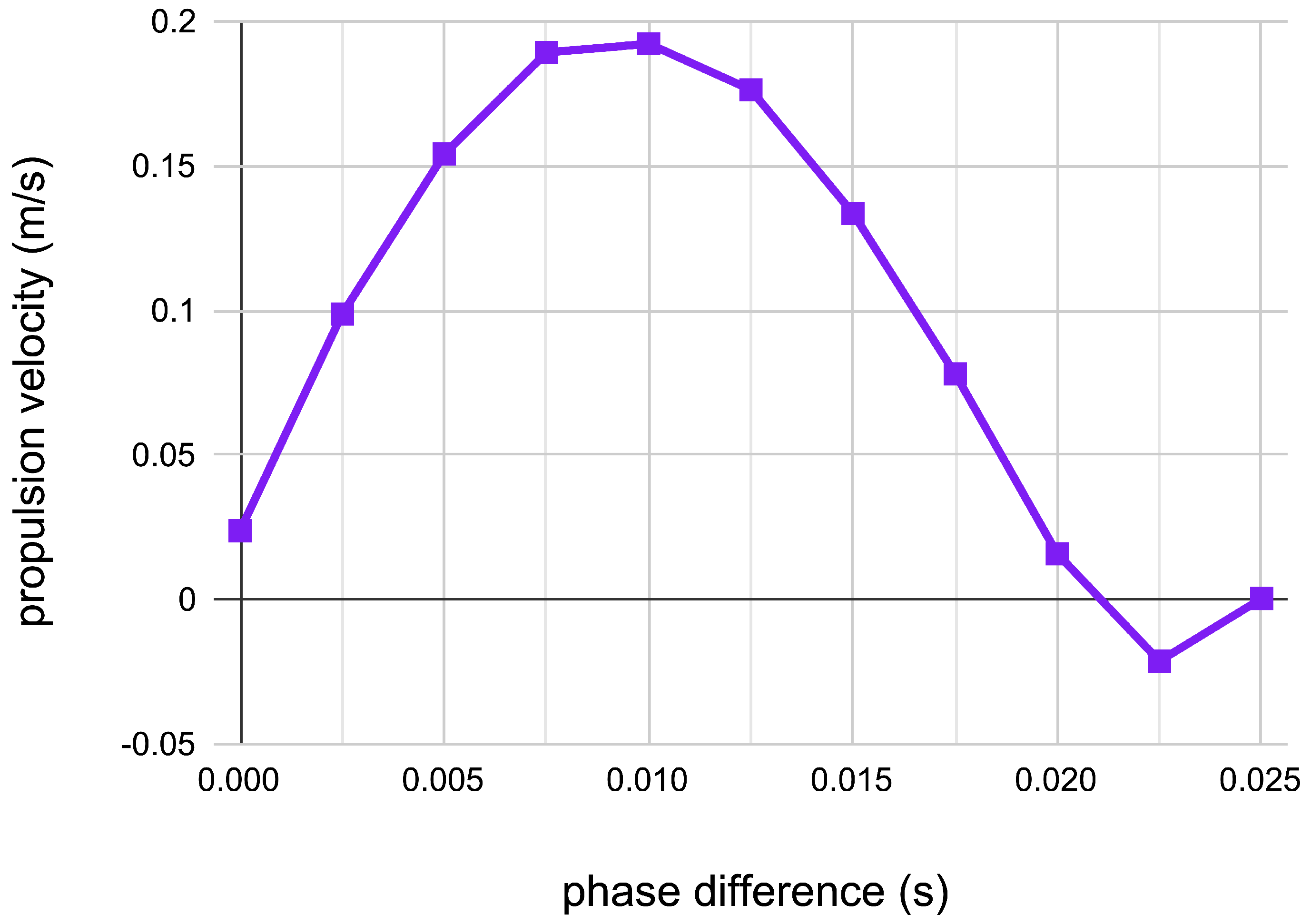
The simulation was performed over a range of phase differences between 0 and with the configuration outlined in Section 2. An increment of between trials was used. The average horizontal propulsion velocities for each phase difference is shown below in Figure 4.
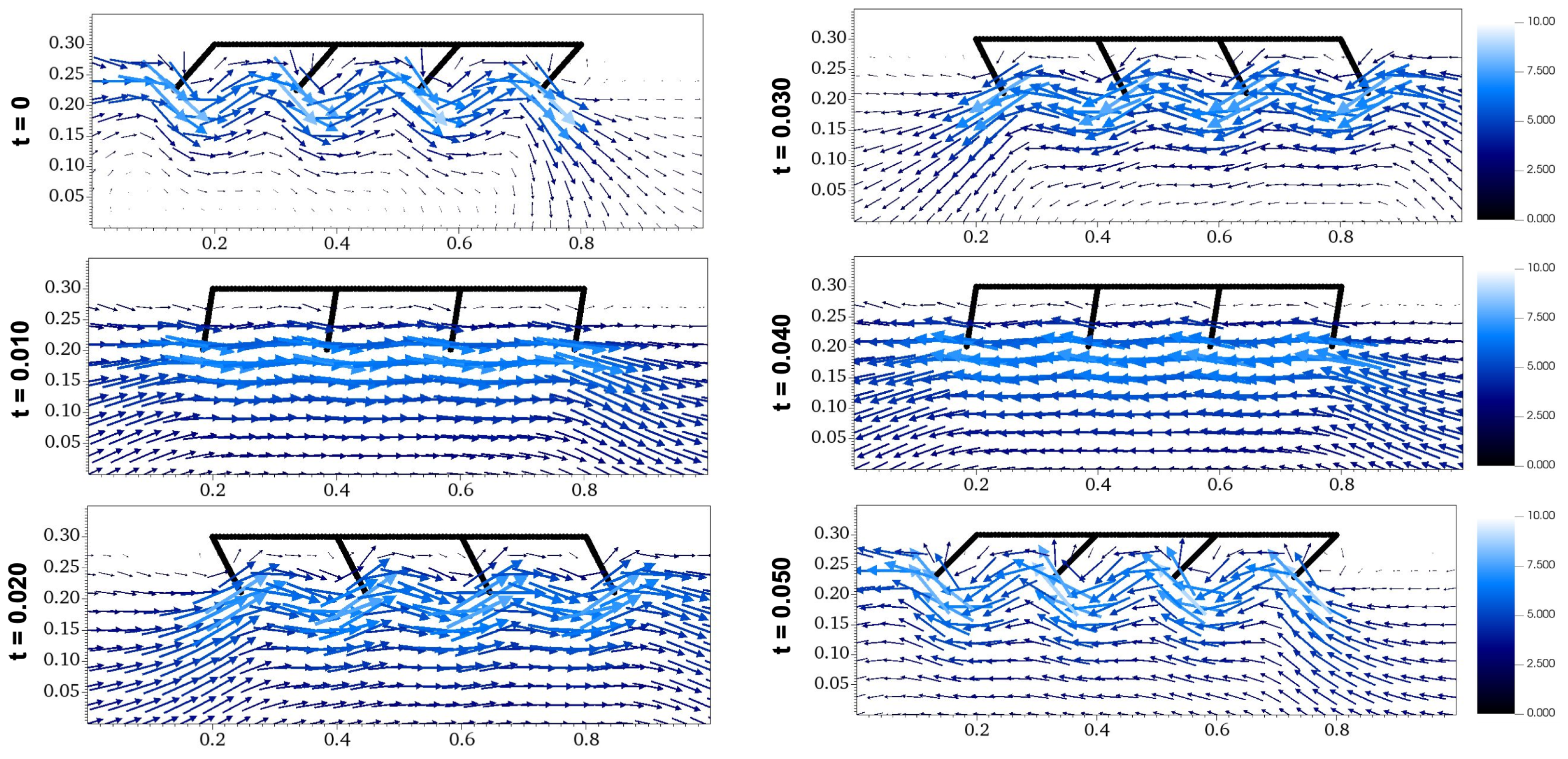
Figure 5 depicts six frames of the crustacean model’s metachronal motion with , taken in increments of 0.010 s over one full period. From t = 0 s to t = 0.025 s, all paddles underwent the power stroke, and from t = 0.025 s to t = 0.050 s, they underwent the return stroke. This shift in direction is shown by the velocity vectors of the surrounding fluid, as they switched in direction from t = 0.020 s to t = 0.030 s. Since the phase shift was 0 s, Figure 5 shows synchronous motion, which had all four paddles moving in unison. Figure 6 shows six frames of metachronal motion with between paddles, which was asynchronous motion because the paddles were not in the same phase at the same time. As discussed later in Section 4.1, the difference between the resulting velocities of synchronous and asynchronous motion are significant because asynchronous motion causes a large increase in propulsion when compared to synchronous motion.
3.2. Effect of Body Morphology on Velocity
We simulated the 2D crustacean model via IB2d with varying body morphologies. To do so, we adjusted the value of k and, therefore, the body shape while holding constant at .
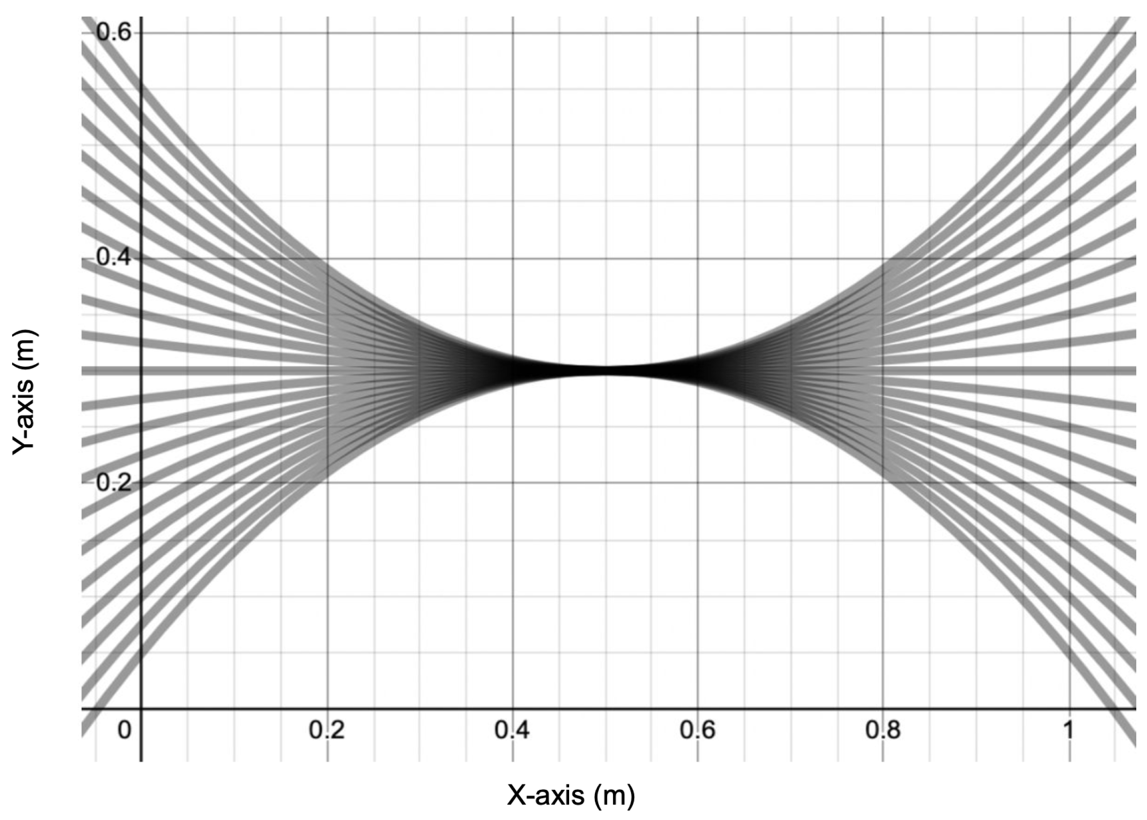
With the methodology outlined in Section 2, the simulation was performed over a range of body morphologies, represented by the interval and shown in Figure 7. Due to the behavior of parabolas, the crustacean body will assume an upwards curve (convex) when and a downwards curve (concave) when . We incremented k by 0.1 between trials to obtain a comprehensive graph with 21 data points.
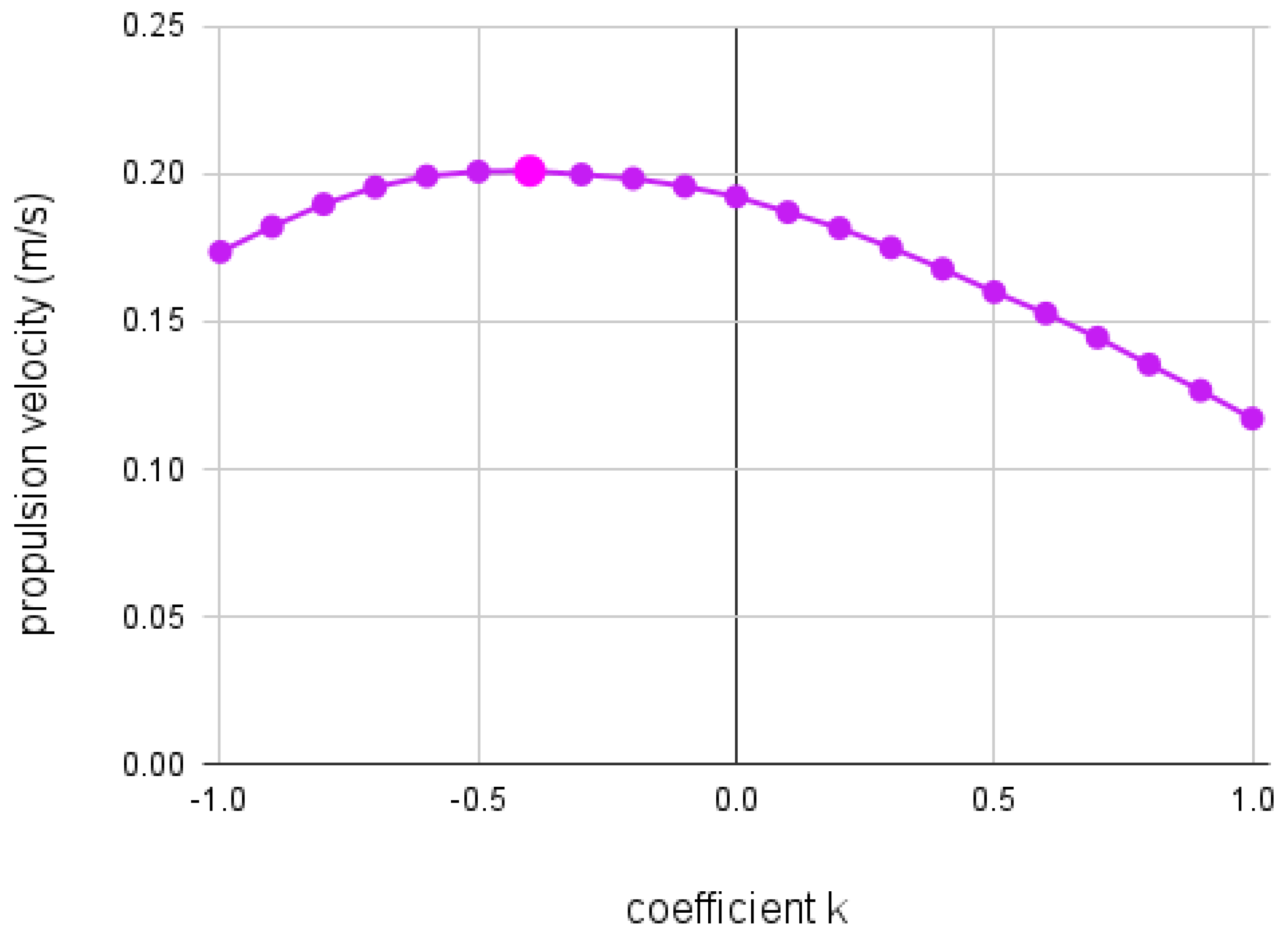
Figure 8 presents the relation between k and . As k increases from −1, the propulsion velocity steadily rises with negative concavity, peaking when k equals −0.4. Then, steadily decreases as k increases to 1. The results showed that propulsion velocity is maximized when , when the crustacean’s body is a slight downward curve described by the equation .
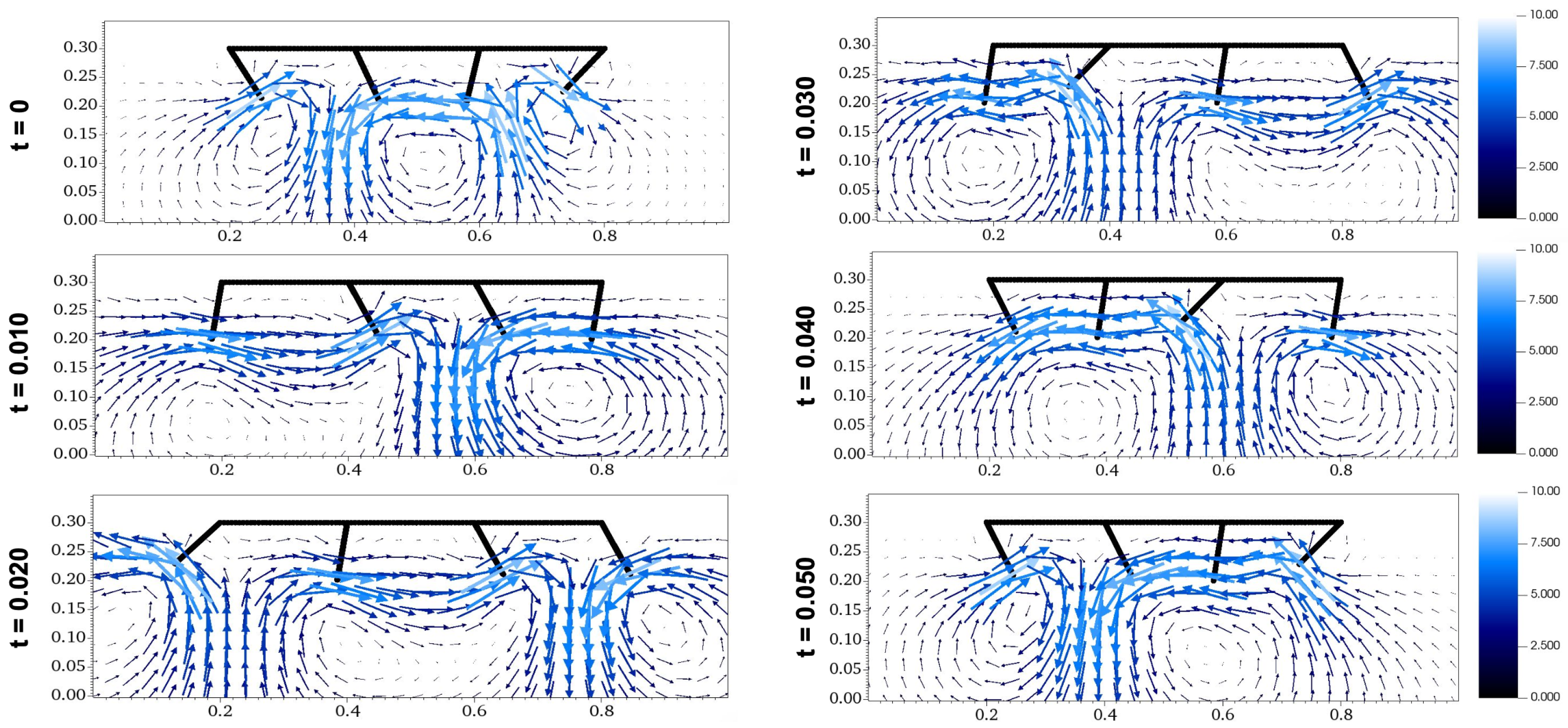
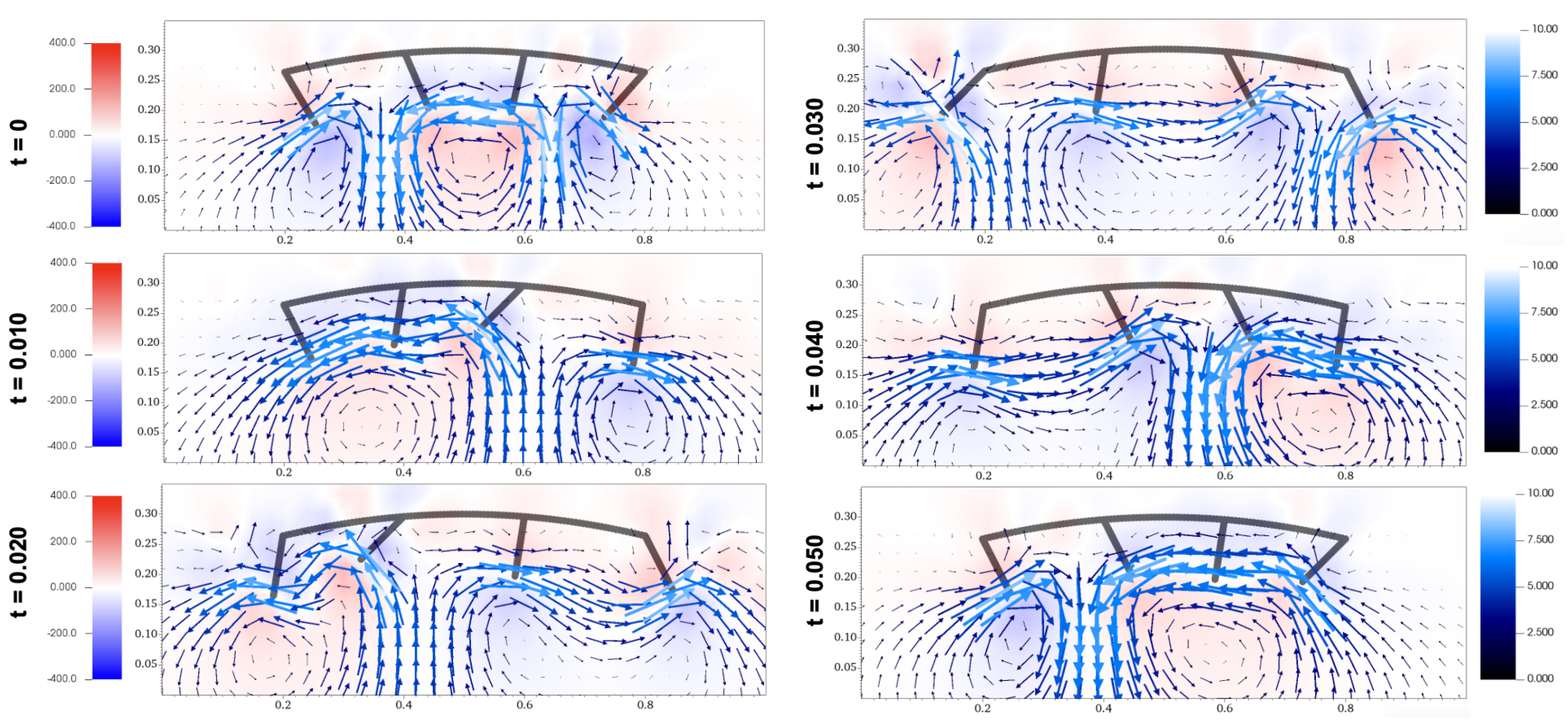
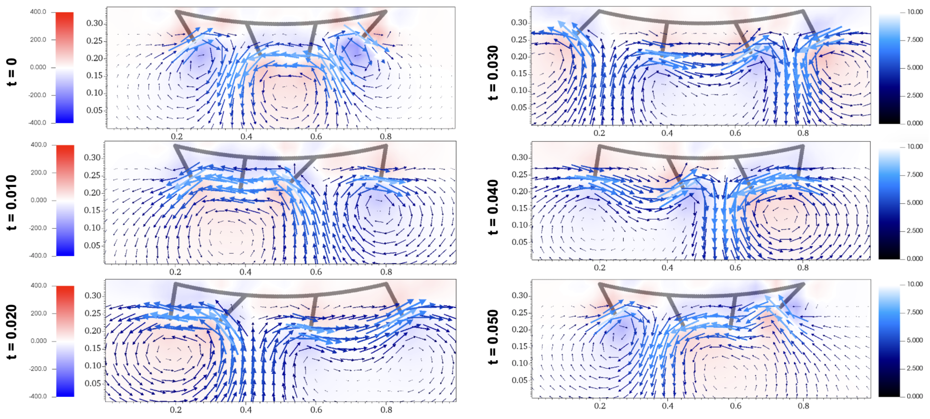
Figure 9 depicts six frames of the crustacean model’s metachronal motion with , taken in increments of 0.010 s over one full period. Since k is negative here, the crustacean morphology resembles a downwards curve. Figure 10 shows six frames of metachronal motion with , which yields an upward curve. Both of these flow diagrams were simulated with , the phase shift that optimizes horizontal velocity.
4. Discussion
The results revealed that a curved downwards morphology achieved superior metachronal propulsion.
4.1. Effect of Phase Difference
The phase difference of metachronal locomotion heavily impacted the resulting propulsion velocity, optimized at , as shown in Figure 4. While metachronal motion with produced a velocity of 0.016 m/s, metachronal motion with achieved velocities upwards of 0.192 m/s, an increase of more than 1200% in speed. Adjustments of the phase shift in the interval from 0 to 0.025 were shown to yield a wide range of velocities, including negative, zero, and positive. As the phase difference increased from 0, the propulsion velocity steadily grew before plateauing at 0.01, decreasing gradually until reaching zero at . The results showed that was maximized at s, or when each swimmeret differed by 20% of the period in motion. This trend agrees with the figures and results introduced in [9,13,15] for antiplectic metachronal propulsion. Additionally, the negative propulsion velocity from a phase difference of 0.0225 was previously produced by [13]. Thus, creating a phase difference between appendages enhances velocity and efficiency in crustaceans and cilia. To visually see the difference between synchronous and asynchronous movement, please refer to the fluid simulations Videos S1 and S2 in the Supplemental Materials.
4.2. Effect of Morphology
Our results showed the significance of morphology on velocity from metachronal propulsion. By comparing the propulsion velocities over a range of different nonlinear morphologies, we found that a downwards parabola with a leading coefficient of −0.4 maximized the propulsion velocity, achieving a time-averaged mean 4.5% greater than the velocity of the linear model. As shown in Figure 8, adjusting the coefficient k resulted in a range of different propulsion velocities. Over the range of to 1 in increments of , the value of k influenced the propulsion velocity, as shown by how at varied by 39% from at . Overall, Figure 8 resembles a wide downward curve that achieved maximum propulsion velocity at , which corresponds to a downward parabola. Compared to the linear morphology, when , a nonlinear morphology with resulted in a increase in velocity. While not necessarily optimal, morphologies with k values between and outperformed the linear morphology in terms of propulsion velocity as well.
Comparing the flow diagram between Figure 9 and Figure 10 at s and s, the waves created by the paddles interacted differently. With a downwards morphology of , the movement of the last paddle carried the wave backwards in a downwards manner at time s, while the upwards morphology of resulted in the wave being carried in a higher direction. At s, the last paddle in the morphology with created a wave below the preexisting wave, while the last paddle in the morphology with created a wave around the same height as the preexisting wave. These differences occur throughout the fluid simulations for Figure 9 and Figure 10, which can be accessed as Videos S3 and S4. These examples show how the favorable orientation and interaction of waves in the morphology with contributed to its higher propulsion velocity.
Another explanation for the superior performance of the downwards parabola is that the curved border allows for improved wave propagation and fluid transport. The additional space provided by the morphology might reduce interference for metachronal waves, which then creates increased propulsion.
5. Conclusions
In both CFD and robotic models, previous research simplified simulating metachronal movement by implementing a linear body. However, this is not the case for cilia or crustaceans; cilia extend off a curved cell surface, and crustaceans do not swim perfectly straight. By introducing a way of altering the morphology, we brought an additional dimension of biological accuracy to research in metachronal propulsion. In this study, we assessed the impact of the phase difference and morphology on metachronal propulsion. The simulations on the phase difference showed that propulsion is maximized at . Additionally, it can be concluded that the phase shift plays a significant role in determining the efficiency of metachronal movement, capable of yielding speeds 800% of those from non-metachronal movement. Simulations for nonlinear morphologies revealed that the downwards parabolic curve with variable yields optimal metachronal propulsion, 4.5% greater than its nonlinear equivalent. Further, within the interval , the corresponding morphologies have large effects on metachronal propulsion. One such curved morphology resulted in 30% less velocity than the linear model, given that the phase shift is constant. These results contribute to the body of knowledge in bio-inspired fluid mechanics and metachronal movement. Comprehension of this topic can lead to the development of new nanotechnology or marine exploration technology by introducing a new method of efficient swimming.
6. Future Research
The techniques and models used in this study can benefit from future iterations and extensions. A generalized parabola equation was used to generate morphologies. Future research may look into methods of generating a larger variety of morphologies or creating an adaptive method to find the optimal shape for metachronal propulsion. Another consideration for future studies in morphology and metachrony is investigating the best way to position paddles on different morphologies. This study placed paddles at x-coordinates of , and regardless of the body shape. This method of keeping paddle–body intersection points constant could alter more variables than expected. For example, the spacing between crustacean appendages was altered, increasing between paddles 1 and 2, but decreasing between paddles 2 and 3. Implementing additional walls for the crustacean body and flexible paddles will allow for more realistic configurations. The development of flexible paddles is especially pivotal, as the movement of crustaceans is altered by the jointed nature of the swimmerets. Our method features a simple process of generating paddle coordinates, but more research could yield a standardized procedure for placing paddles on nonlinear morphologies. Expanding the results of this study from 2D simulations to 3D simulations will allow for the modeling of more-complex and -realistic crustacean biology, as well as improving visualization.
Supplementary Materials
The following Supporting Information is available at https://www.mdpi.com/article/10.3390/fluids9010002/s1, Video S1: Fluid simulation for the crustacean morphology with k = 0 and phase change = 0 s. Video S2: Fluid simulation for the crustacean morphology with k = 0 and phase change = 0.010 s. Video S3: Fluid simulation for the crustacean morphology with k = −0.4 and phase change = 0.010 s. Video S4: Fluid simulation for the crustacean morphology with k = 0.4 and phase change = 0.010 s.
Author Contributions
Conceptualization, E.C. and Z.J.K.; data curation, E.C.; formal analysis, E.C.; investigation, E.C. and Z.J.K.; methodology, E.C. and Z.J.K.; project administration, E.C.; resources, E.C. and Z.J.K.; supervision, Z.J.K.; validation, E.C. and Z.J.K.; visualization, E.C. and Z.J.K.; writing—original draft, E.C. and Z.J.K.; writing—review and editing, E.C. and Z.J.K. All authors have read and agreed to the published version of the manuscript.
Funding
This research received no external funding.
Data Availability Statement
Data files for simulations are available upon reasonable request.
Acknowledgments
We acknowledge three anonymous reviewers for their careful reading of our initial manuscript and for offering constructive and insightful critiques, which allowed us to significantly improve the manuscript.
Conflicts of Interest
The authors declare no conflicts of interest.
Abbreviations
The following abbreviations are used in this manuscript:
| CFD | Computational fluid dynamics |
| Re | Reynolds number |
| PS | Power stroke |
| RS | Return/recovery stroke |
References
- Lauder, G.V. Fish Locomotion: Recent Advances and New Directions. Annu. Rev. Mar. Sci. 2015, 7, 521–545. [Google Scholar] [CrossRef] [PubMed]
- Zhu, Q. Physics and applications of squid-inspired jetting. Bioinspir. Biomim. 2022, 17, 041001. [Google Scholar] [CrossRef] [PubMed]
- Purcell, E.M. Life at low Reynolds number. Am. J. Phys. 1977, 45, 3–11. [Google Scholar] [CrossRef]
- Ford, M.P.; Lai, H.K.; Samaee, M.; Santhanakrishnan, A. Hydrodynamics of metachronal paddling, effects of varying Reynolds number and phase lag. R. Soc. Open Sci. 2019, 6, 191387. [Google Scholar] [CrossRef] [PubMed]
- Hayashi, R.; Takagi, D. Metachronal Swimming with Rigid Arms near Boundaries. Fluids 2020, 5, 24. [Google Scholar] [CrossRef]
- Kohlhage, K.; Yager, J. An analysis of swimming in remipede crustaceans. Philos. Trans. R. Soc. B Biol. Sci. 1994, 346, 213–221. [Google Scholar] [CrossRef]
- Lim, J.L.; DeMont, M.E. Kinematics, hydrodynamics and force production of pleopods suggest jet-assisted walking in the American lobster (Homarus americanus). J. Exp. Biol. 2009, 212, 2731–2745. [Google Scholar] [CrossRef] [PubMed]
- Elgeti, J.; Gompper, G. Emergence of metachronal waves in cilia arrays. Proc. Natl. Acad. Sci. USA 2013, 110, 4470–4475. [Google Scholar] [CrossRef]
- Milana, E.; Zhang, R.; Vetrano, M.R.; Peerlinck, S.; Volder, M.D.; Onck, P.R.; Reynaerts, D.; Gorissen, B. Metachronal patterns in artificial cilia for low Reynolds number fluid propulsion. Sci. Adv. 2020, 6, eabd2508. [Google Scholar] [CrossRef]
- Byron, M.L.; Murphy, D.W.; Katija, K.; Hoover, A.P.; Daniels, J.; Garayev, K.; Takagi, D.; Kanso, E.; Gemmell, B.J.; Ruszczyk, M.; et al. Metachronal Motion across Scales: Current Challenges and Future Directions. Integr. Comp. Biol. 2021, 61, 1674–1688. [Google Scholar] [CrossRef]
- Mulloney, B.; Smarandache-Wellmann, C. Neurobiology of the crustacean swimmeret system. Prog. Neurobiol. 2012, 96, 242–267. [Google Scholar] [CrossRef] [PubMed]
- Laverack, M.S.; Macmillan, D.L.; Neil, D.M. A comparison of beating parameters in larval and post-larval locomotor systems of the lobster Homarus gammarus (L.). Philos. Trans. R. Soc. B Biol. Sci. 1976, 274, 87–99. [Google Scholar] [CrossRef]
- Grazier-Nakajima, S.; Guy, R.D.; Zhang-Molina, C. A Numerical Study of Metachronal Propulsion at Low to Intermediate Reynolds Numbers. Fluids 2020, 5, 86. [Google Scholar] [CrossRef]
- Murphy, D.W.; Webster, D.R.; Kawaguchi, S.; King, R.; Yen, J. Metachronal swimming in Antarctic krill: Gait kinematics and system design. Mar. Biol. 2011, 158, 2542–2554. [Google Scholar] [CrossRef]
- Zhang, C.; Guy, R.D.; Mulloney, B.; Zhang, Q.; Lewis, T.J. Neural mechanism of optimal limb coordination in crustacean swimming. Proc. Natl. Acad. Sci. USA 2014, 111, 13840–13845. [Google Scholar] [CrossRef] [PubMed]
- Alben, S.; Spears, K.; Garth, S.; Murphy, D.; Yen, J. Coordination of multiple appendages in drag-based swimming. J. R. Soc. Interface 2010, 7, 1545–1557. [Google Scholar] [CrossRef]
- Alexander, D.E. Kinematics of swimming in two species of Idotea (Isopoda: Valvifera). J. Exp. Biol. 1988, 138, 37–49. [Google Scholar] [CrossRef]
- Daniels, J.; Aoki, N.; Havassy, J.; Katija, K.; Osborn, K. Metachronal Swimming with Flexible Legs: A Kinematics Analysis of the Midwater Polychaete Tomopteris. Integr. Comp. Biol. 2021, 61, 1658–1673. [Google Scholar] [CrossRef]
- Hanasoge, S.; Hesketh, P.; Alexeev, A. Metachronal Acutation of Microscale Magnetic Artificial Cilia. Am. Chem. Soc. Appl. Mater. Interfaces 2020, 12, 46963–46971. [Google Scholar] [CrossRef]
- Khaderi, S.N.; den Toonder, J.M.J.; Onck, P.R. Microfluidic propulsion by the metachronal beating of magnetic artificial cilia: A numerical analysis. J. Fluid Mech. 2011, 688, 44–65. [Google Scholar] [CrossRef]
- Ford, M.P.; Santhanakrishnan, A. Closer Appendage Spacing Augments Metachronal Swimming Speed by Promoting Tip Vortex Interactions. Integr. Comp. Biol. 2021, 61, 1608–1618. [Google Scholar] [CrossRef] [PubMed]
- Ford, M.P.; Ray, W.K.; DiLuca, E.M.; Patek, S.N.; Santhanakrishnan, A. Hybrid Metachronal Rowing Augments Swimming Speed and Acceleration via Increased Stroke Amplitude. Integr. Comp. Biol. 2021, 61, 1619–1630. [Google Scholar] [CrossRef] [PubMed]
- Wang, A.X.G.; Kabala, Z.J. Body Morphology and Drag in Swimming: CFD Analysis of the Effects of Differences in Male and Female Body Types. Fluids 2022, 7, 332. [Google Scholar] [CrossRef]
- Sun, H.; Ding, W.; Zhao, X.; Sun, Z. Numerical Study of Flat Plate Impact on Water Using a Compressible CIP–IBM–Based Model. J. Mar. Sci. Eng. 2022, 10, 1462. [Google Scholar] [CrossRef]
- Jiang, H. Numerical Simulation of Self-Propelled Steady Jet Propulsion at Intermediate Reynolds Numbers: Effects of Orifice Size on Animal Jet Propulsion. Fluids 2021, 6, 230. [Google Scholar] [CrossRef]
- Kim, D.-H.; Park, J.-C.; Jeon, G.-M.; Shin, M.-S. CFD Simulation for Estimating Efficiency of PBCF Installed on a 176K Bulk Carrier under Both POW and Self-Propulsion Conditions. Processes 2021, 9, 1192. [Google Scholar] [CrossRef]
- Ding, Y.; Kanso, E. Selective particle capture by asynchronously beating cilia. Phys. Fluids 2015, 27, 121902. [Google Scholar] [CrossRef]
- Chateau, S. Why anti-plectic metachronal cilia are optimal to transport bronchial mucus. Phys. Rev. E 2019, 100, 042405. [Google Scholar] [CrossRef]
- Brennen, C. An oscillating-boundary-layer theory for ciliary propulsion. J. Fluid Mech. 1974, 65, 799–824. [Google Scholar] [CrossRef]
- Peskin, C.S. Flow patterns around heart valves: A numerical method. J. Comput. Phys. 1972, 10, 252–271. [Google Scholar] [CrossRef]
- Lauga, E.; Powers, T.R. The hydrodynamics of swimming microorganisms. Annu. Rev. Fluid Mech. 2009, 41, 105–139. [Google Scholar] [CrossRef]
- Miles, J.G.; Battista, N.A. Naut Your Everyday Jellyfish Model: Exploring How Tentacles and Oral Arms Impact Locomotion. Fluids 2019, 4, 169. [Google Scholar] [CrossRef]
- Battista, N.A.; Baird, A.J.; Miller, L.A. A Mathematical Model and MATLAB Code for Muscle-Fluid-Structure Simulations. Integr. Comp. Biol. 2015, 55, 901–911. [Google Scholar] [CrossRef] [PubMed]
- Battista, N.A.; Strickland, W.C.; Miller, L.A. IB2d: A Python and MATLAB implementation of the immersed boundary method. Bioinspir. Biomim. 2016, 12, 036003. [Google Scholar] [CrossRef]
- Senter, D.M.; Douglas, D.R.; Strickland, W.C.; Thomas, S.G.; Talkington, A.M.; Miller, L.A.; Battista, N.A. A semi-automated finite difference mesh creation method for use with immersed boundary software IB2d and IBAMR. Bioinspir. Biomim. 2021, 16, 016008. [Google Scholar] [CrossRef]
- Battista, N.A.; Strickland, W.C.; Barrett, A.; Miller, L.A. IB2d Reloaded: A more powerful Python and MATLAB implementation of the immersed boundary method. Math. Methods Appl. Sci. 2017, 41, 8455–8480. [Google Scholar] [CrossRef]
Figure 1.
A marsh grass shrimp (Palaemonetes vulgaris) performing metachronal swimming. This figure is displayed under the Creative Commons CC BY-SA 3.0 License. Image courtesy of Nils Tack/University of South Florida.
Figure 1.
A marsh grass shrimp (Palaemonetes vulgaris) performing metachronal swimming. This figure is displayed under the Creative Commons CC BY-SA 3.0 License. Image courtesy of Nils Tack/University of South Florida.

Figure 2.
A schematic of a sample crustacean model. Some indicated features include labeled power strokes and return strokes, the swimming direction, paddle spacing, and each paddle’s range of motion.
Figure 2.
A schematic of a sample crustacean model. Some indicated features include labeled power strokes and return strokes, the swimming direction, paddle spacing, and each paddle’s range of motion.

Figure 3.
A comparison between the grid width, , and the simulated propulsion velocity.

Figure 4.
Propulsion velocity () vs. phase difference () over the range of 0 .

Figure 5.
Flow diagrams of metachronal propulsion with a synchronous paddle motion.

Figure 6.
Flow diagrams of metachronal propulsion with , an asynchronous paddle motion.

Figure 7.
A graphical representation of the tested range of crustacean morphology, with .

Figure 8.
Propulsion velocity () vs. coefficient k over the range of −1 1.

Figure 9.
Flow diagrams of metachronal propulsion including vorticity with , which ensures maximum .
Figure 9.
Flow diagrams of metachronal propulsion including vorticity with , which ensures maximum .

Figure 10.
Flow diagrams of metachronal propulsion including vorticity with .


Table 1.
The effect of confirmatory phase difference values on propulsion velocity.
| (s) | () |
|---|---|
| 0 | 0.0238 |
| 0.01 | 0.1539 |
| 0.025 | 0.0004 |
Disclaimer/Publisher’s Note: The statements, opinions and data contained in all publications are solely those of the individual author(s) and contributor(s) and not of MDPI and/or the editor(s). MDPI and/or the editor(s) disclaim responsibility for any injury to people or property resulting from any ideas, methods, instructions or products referred to in the content. |
© 2023 by the authors. Licensee MDPI, Basel, Switzerland. This article is an open access article distributed under the terms and conditions of the Creative Commons Attribution (CC BY) license (https://creativecommons.org/licenses/by/4.0/).
Share and Cite
MDPI and ACS Style
Cao, E.; Kabala, Z.J. Impact of Crustacean Morphology on Metachronal Propulsion: A Numerical Study. Fluids 2024, 9, 2. https://doi.org/10.3390/fluids9010002
AMA Style
Cao E, Kabala ZJ. Impact of Crustacean Morphology on Metachronal Propulsion: A Numerical Study. Fluids. 2024; 9(1):2. https://doi.org/10.3390/fluids9010002
Chicago/Turabian StyleCao, Enbao, and Zbigniew J. Kabala. 2024. "Impact of Crustacean Morphology on Metachronal Propulsion: A Numerical Study" Fluids 9, no. 1: 2. https://doi.org/10.3390/fluids9010002