
On the Composite Velocity Profile in Zero Pressure Gradient Turbulent Boundary Layer: Comparison with DNS Datasets

1
Hydromechanics and Environmental Engineering Laboratory, Department of Civil Engineering, University of Thessaly, Pedion Areos, 38334 Volos, Greece
2
Condensed Matter Physics Laboratory, Department of Physics, University of Thessaly, 35100 Lamia, Greece
*
Author to whom correspondence should be addressed.
Fluids 2023, 8(10), 260; https://doi.org/10.3390/fluids8100260
Submission received: 1 August 2023
/
Revised: 10 September 2023
/
Accepted: 20 September 2023
/
Published: 25 September 2023
(This article belongs to the Special Issue Next-Generation Methods for Turbulent Flows)
Abstract
:Data obtained by direct numerical simulations (DNS) of the Zero-Pressure-Gradient Turbulent Boundary Layer were analyzed and compared to a mathematical model of the mean velocity profile (MVP) in the range 1000 ≤ Reθ ≤ 6500. The mathematical model is based on the superposition of an accurate description of the inner law and Coles’ wake function with appropriately chosen parameters. It is found that there is excellent agreement between the mathematical model and the DNS data in the inner layer when the Reynolds number based on momentum thickness, Reθ, is greater than 1000. Furthermore, there is very good agreement over the entire boundary layer thickness, when Reθ is greater than 2000. The diagnostic functions Ξ and Γ based on DNS data are examined and their characteristics are discussed in relation to the existence of a logarithmic layer or a power law behavior of the MVP. The diagnostic functions predicted by the mathematical model are also presented.
1. Introduction
In the framework of Computational Fluid Mechanics, turbulent flows are usually simulated using the Reynolds Averaged Navier Stokes (RANS) equations, augmented by empirical turbulence models, which were calibrated with experimental data of simple turbulent flows and contain several simplifying assumptions. These disadvantages can be avoided by using the direct numerical simulation (DNS) methodology. The DNS method is considered to be capable of resolving even the smallest eddies on the spatial and temporal scales of turbulence. This requires the use of extremely dense grids, making DNS solutions costly in terms of computation time and memory. Although the DNS method does not require additional turbulence closure equations, it creates the need for very dense computational grids as well as extremely small integration time—steps in order to achieve accurate solutions. Consequently, the scope of the DNS method is currently limited to flows with relatively low Reynolds numbers [1,2,3].
In the context of routine engineering applications, an accurate and convenient method of calculating the average velocity profile is often sufficient. By “convenient method”, we mean that three conditions should be satisfied: that the profile is given in the form of a closed mathematical expression, that the velocity is given explicitly as a function of the wall distance, i.e., as a function u(y) and not in an implicit form y(u), and that the interval of validity of the mathematical expression covers the entire thickness of the boundary layer. In this paper, we briefly describe a mathematical model which has been originally introduced by Liakopoulos [4]. For convenience, the model will be referred to as the AL84 model in the remainder of the paper. Naturally, the accuracy of a model must first be documented by the verification and validation process, through comparison with experimental or DNS data. In the present work, we focus on comparisons with DNS results. The model will be described, verified, and validated for two—dimensional incompressible turbulent boundary layer flows, developing on smooth surfaces with zero pressure gradient. The model can be generalized to describe boundary layers growing under the influence of pressure gradient, positive or negative.
2. Modelling the Mean Velocity Profile Methodology
The standard model of the turbulent boundary layer is the three-zone model which includes the inner zone, the outer zone, and the overlap zone where the logarithmic law applies. We remind the reader that for the mathematical description of the inner zone, suitable variables are y+ = and u+ = , where y is the distance normal to the solid surface, u is the velocity component in the main direction of flow, ν is the kinematic viscosity coefficient and uτ is the shear velocity at the wall [5,6]. It is worth pointing out that the logarithmic law u+ = lny+ + Β is valid in the interval [, ]. The values of and depend on the value of the Reynolds number Reθ (defined by the boundary layer momentum thickness θ) and differ between researchers. A common approach when analyzing experimental data for turbulent boundary layer is to use the values κ = 0.40 or 0.41 for von Kármán’s constant and Β = 5.0.
Suitable variables for the mathematical description of the velocity profile in the outer zone are and where δ is the local boundary—layer thickness. Coles [7] analyzed the available experimental measurements and proposed the modeling of the outer layer with a wake function, w, defined by
where
It is important to realize that Equation (1a,b) is the definition of the wake function. At each position y, the value of the function g is the difference between the local time-averaged fluid velocity and the value of the logarithmic law at the same position. The wake function w, defined in Equation (1b), depends on the wake strength parameter Π, which is often referred to as Coles’ parameter. The wake function affects the velocity profile for y+ ≳ 65 and provides an accurate fit to the experimental velocity data for turbulent boundary layers.
To describe mathematically the mean velocity profile on a flat plate over the entire boundary layer thickness we can postulate the existence of a function f that satisfies
In Equation (2), f(y+) is an approximation of the inner law which is valid over the inner layer including the overlap layer. In order for Equations (1) and (2) to be compatible in the outer zone, the function f(y+) must tend asymptotically to the logarithmic law lny+ + Β, for high values of y+. Therefore, to approximate the composite velocity profile, we are required to determine two functions, f and g, whose sum must accurately approximate the velocity u+ for any y+, in the interval [0, δ+].
2.1. Inner Layer
A variety of mathematical expressions of varying levels of complexity and precision have been proposed for the inner law. In this paper, we estimate the accuracy of the AL84 model [4]. In this model, two alternative mathematical expressions for the function f(y+) are proposed:
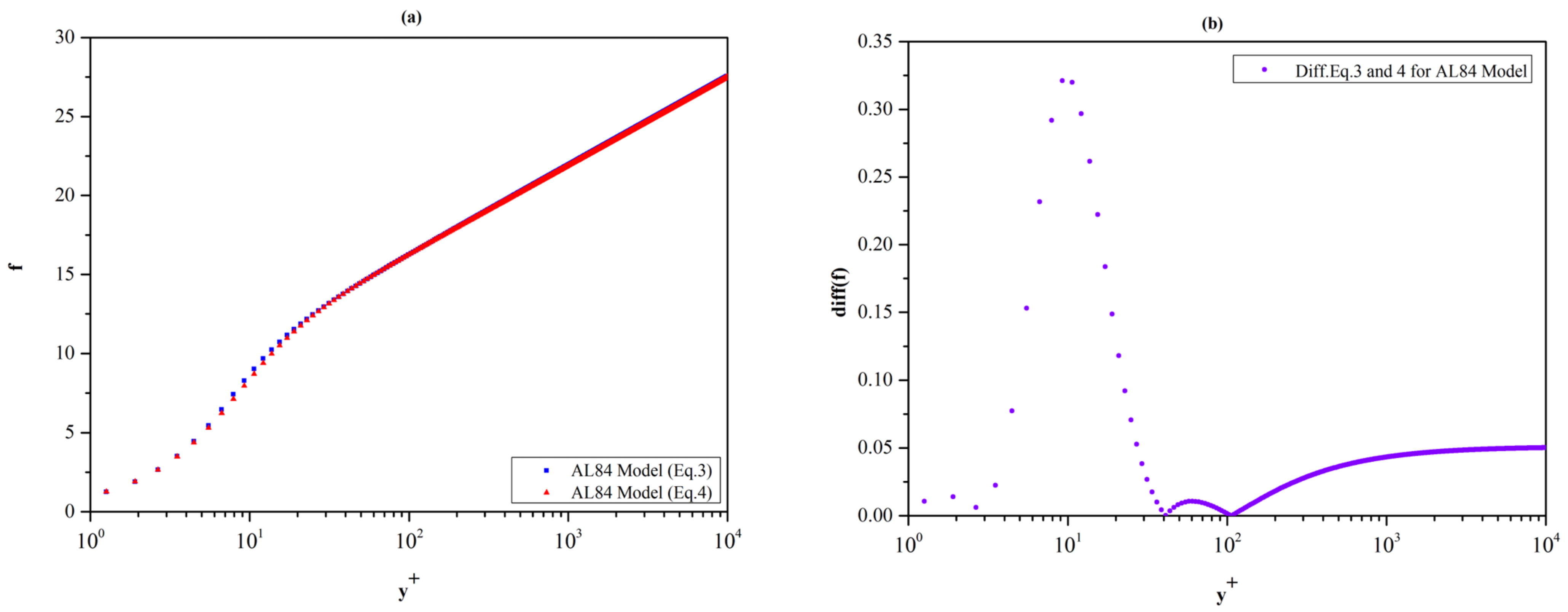
The method of developing Equations (3) and (4) is described in Liakopoulos [4]. In Figure 1 we present the graphs of Equations (3) and (4). It is obvious that the difference between Equations (3) and (4) is rather small, while the maximum of the difference occurs at y+ = 10 and takes the value 0.32. For values of y+ ≥ 50, both functions tend asymptotically to the logarithmic law with κ = 0.41 and B = 5.0, therefore any selection between Equations (3) and (4) has no significant effect on the shape of the mean velocity profile.
2.2. Outer Layer
3. Mean Velocity Profiles
The assessment of the accuracy of the mean velocity profile model is carried out in two stages. The first concerns the interval where the inner law applies, while in the second stage, the comparison is made over the entire thickness of the boundary layer.
3.1. Inner Region: Comparison of f(y+) with ū(y+) Calculated by DNS
In order to confirm the validity of the model, we compare the data of the DNS turbulent boundary layer simulation in a smooth plate with zero pressure gradient of Schlatter and Örlü [13] with the inner law model of AL84.
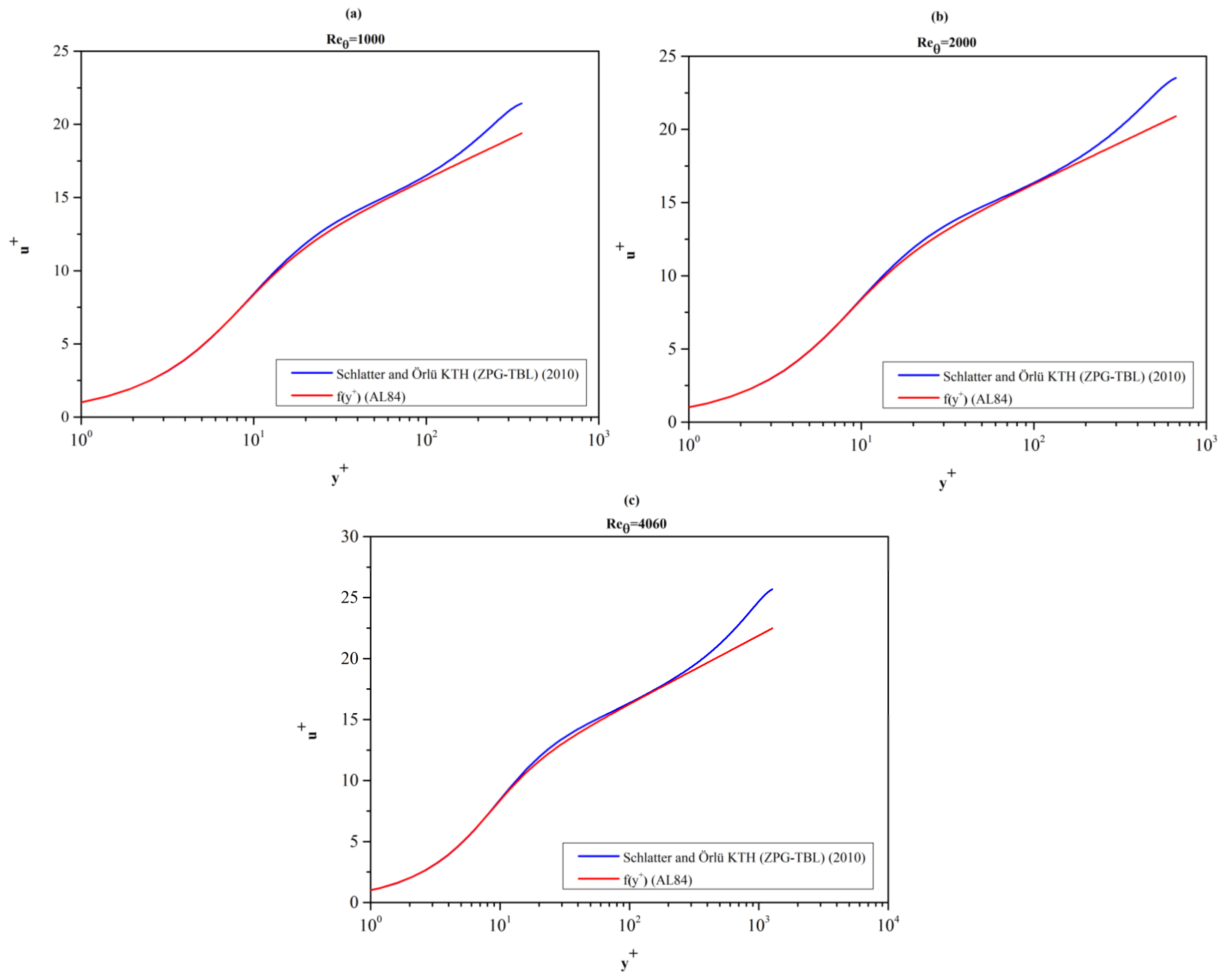
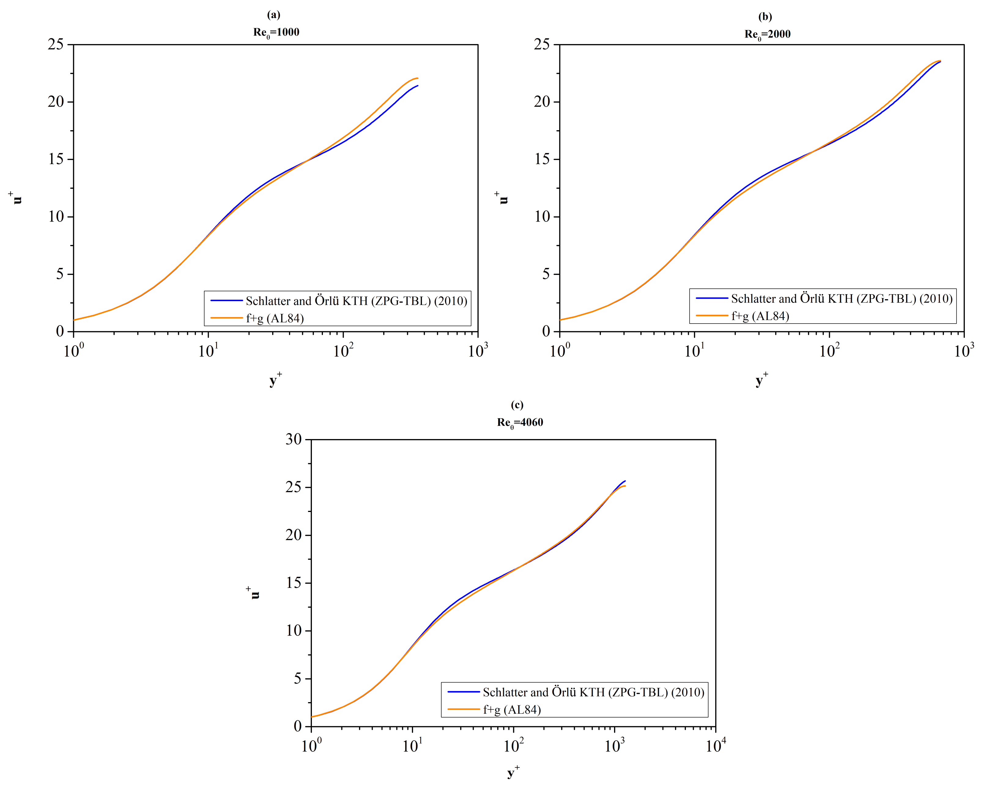
As we described in Section 2.1, Equations (3) or (4) of the AL84 model approximate the mean velocity profile (MVP) in the inner layer i.e., it includes the viscous sublayer, the transition zone, and the overlap zone. In Figure 3, we present a comparison of the time-averaged velocity profiles for the inner law region of the AL84 model and the results of the direct numerical simulation (DNS) of Schlatter and Örlü [13] for three values of Reθ in the range 1000 to 4060. Equation (4) was used to plot the profiles in Figure 3.
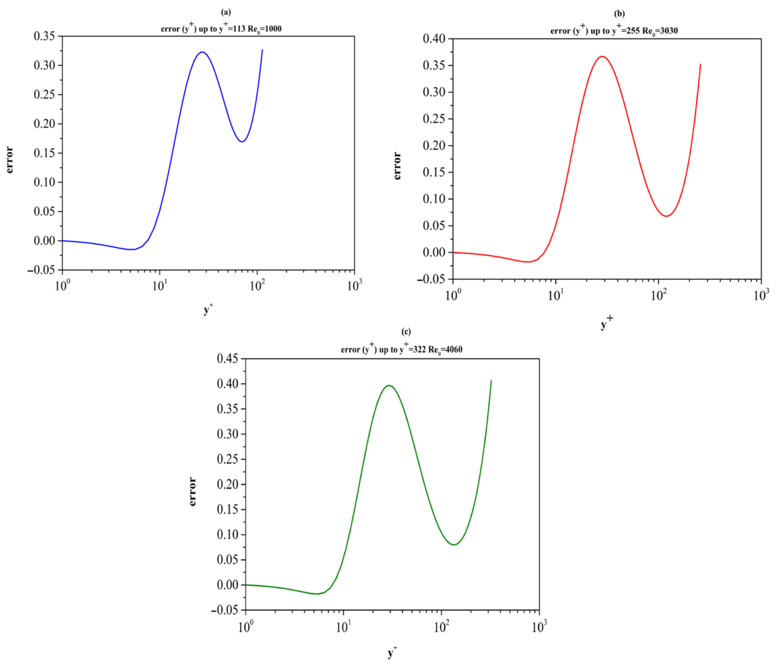
The agreement between the model and the DNS data is excellent and the deviation from the logarithmic law for y+ ≳ 270 (Reθ = 4060) simply demonstrates the need to add the g function (see Section 2.1). The difference [u+(y+) − f(y+)] close to the wall is plotted in Figure 4. The corresponding error statistics are listed in Table 1.
3.2. Comparison of the AL84 Composite Profile (f + g) with DNS Results over the Whole Boundary Layer (0 < y < δ)
In this subsection, we present a comparison of the mean velocity profiles of the numerical results of Schlatter and Örlü [13] and the AL84 composite model over the entire thickness of the boundary layer.
The graphs in Figure 5 show the MVPs of Schlatter and Örlü [13] DNS results for Reθ = 1000, 2000, and 4060. During the evaluation of the AL84 model, κ and Π were assigned values of 0.41 and 0.55, respectively.
The accuracy of the AL84 model is satisfactory for the low Reynolds number Reθ = 1000 and improves significantly as Reθ increases. The agreement for the moderate Reynolds number Reθ = 4060 is excellent. On the scale of Figure 5c, the differences between the two curves are not noticeable except in the interval 20 ≲ y+ ≲ 60.
4. Results Diagnostic Functions
Two distinct diagnostic functions can help to indicate if some portions of a mean velocity profile can be approximated by a logarithmic law or by a power law. Both functions require the calculation of the derivative . The numerical evaluation of the first derivative of u+ with respect to y+ is calculated using the following formula (Equation (7)) for unequally spaced data:
It should be stressed that comparisons in terms of the diagnostic functions present a more stringent check of accuracy since the numerical differentiation of u+(y+) acts as an error amplifier and thus, differences in MVPs are accentuated.
4.1. The Diagnostic Function Ξ
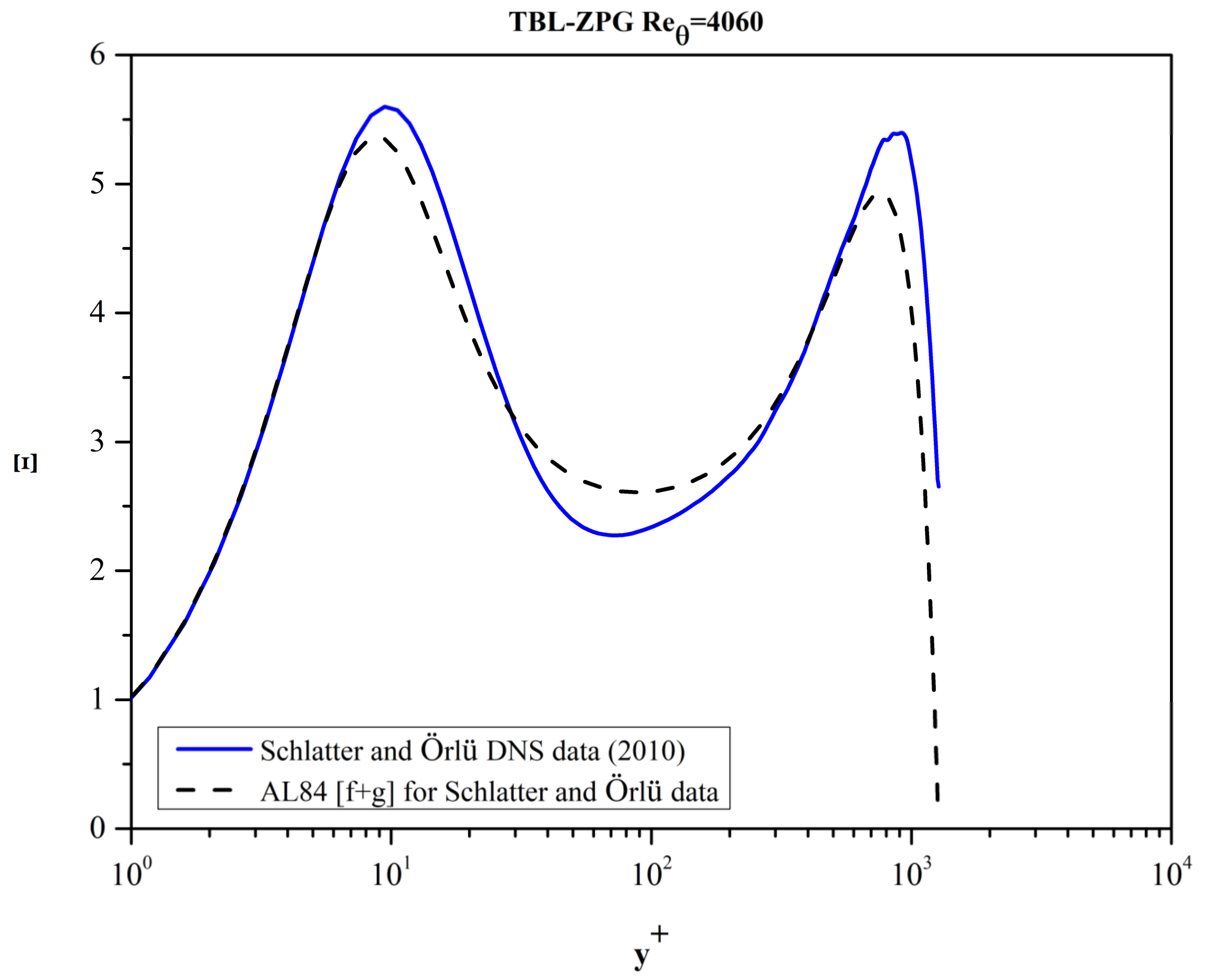
The function Ξ(y+) = y+ serves as a tool for answering some fundamental questions concerning the mathematical form of the inner law. In the first place, as a diagnostic tool, we can easily prove that if a mean velocity profile (MVP) includes an interval [, ] where the classical logarithmic law (see Section 2) holds, then the function Ξ(y+) must attain a constant value, equal to 1/κ, in the interval [, ]. Examining the semi-log plot of function Ξ in Figure 7, we conclude that the MVP reported by Schlatter and Örlü [13] for the moderately large Reθ = 4060 does not exhibit an interval where Ξ(y+) is strictly constant. Thus, the existence of a logarithmic layer is justified only as an approximation in this set of DNS data. This issue is further discussed in Section 4.1.3.
4.1.1. The Diagnostic Function Ξ as Predicted by the AL84 Model
It is worth exploring the behavior of function Ξ as predicted by the AL84 mathematical model for the Schlatter and Örlü [13] data. Referring to Figure 7, we see that the function Ξ reaches approximately a plateau in the interval [65, 135] where it takes the value Ξ = 2.558. Since the existence of the logarithmic law is presupposed in the AL84 model and is incorporated in the construction of the function f of the model with κ = 0.41 (see Section 2) this value is quite close to the expected value. However, it is not exactly equal to 1/0.41 = 2.439. To understand better this difference it is worth studying further the inner workings of the AL84 mathematical model. For completeness of the presentation, we list the parameters of DNS profiles considered in this section in Table 3.
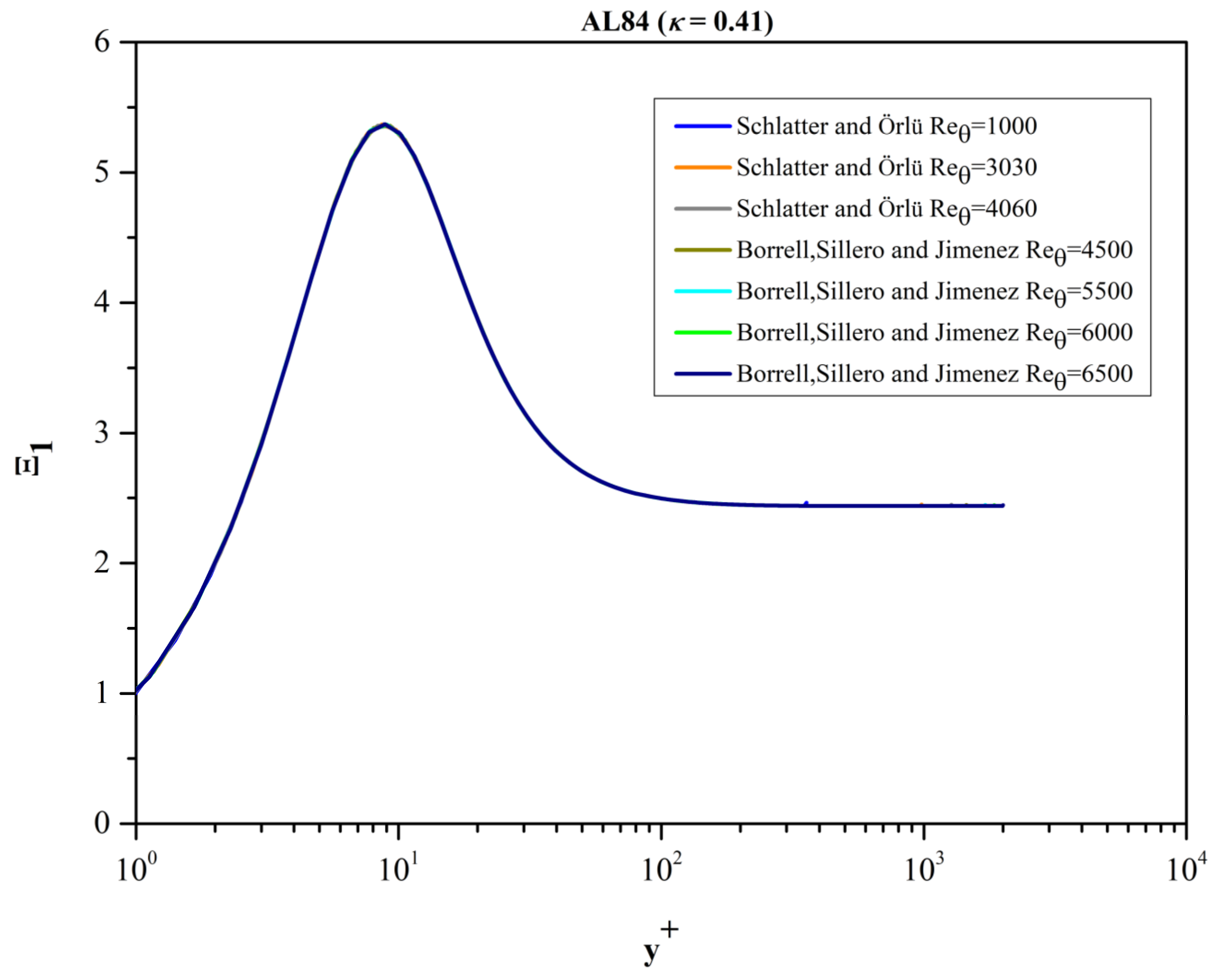
The fact that the validity of a logarithmic law, with parameters κ and Β independent of Reθ, is presupposed in the AL84 model is verified in Figure 8. The function Ξ1 = y+ of AL84 (Equation (4)) is shown for Reθ in the range [1000, 6500]. When y+ ≥ 150, the function Ξ1 becomes equal to 2.45 for all values of Reθ.
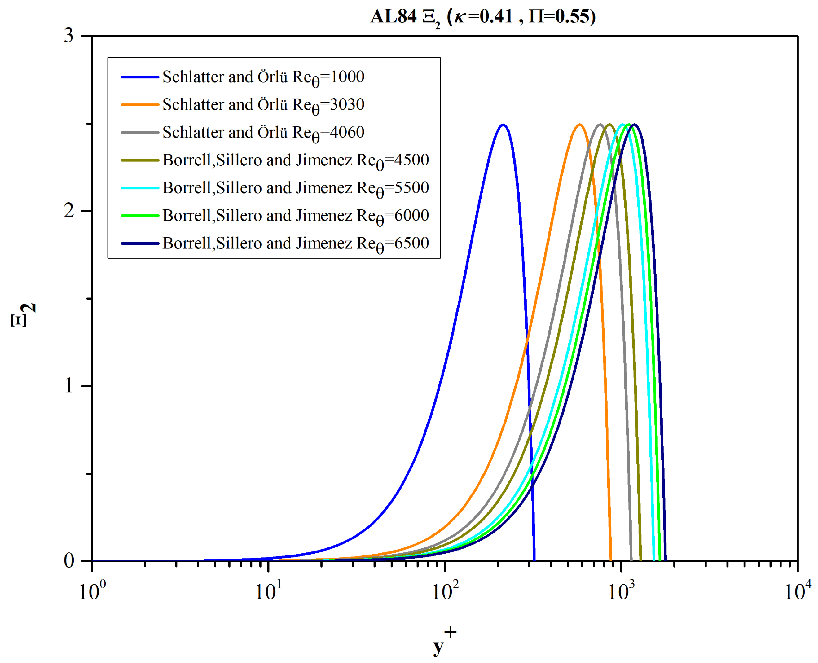
Ideally, the function g (Equation (6)) should not modify the MVP and its derivative close to the wall. In reality, function g has an influence on the inner law for small values of Reθ as can be seen in Figure 9 where Ξ2 = y+ is plotted.
4.1.2. The Function Ξ Based Exclusively on the DNS Data
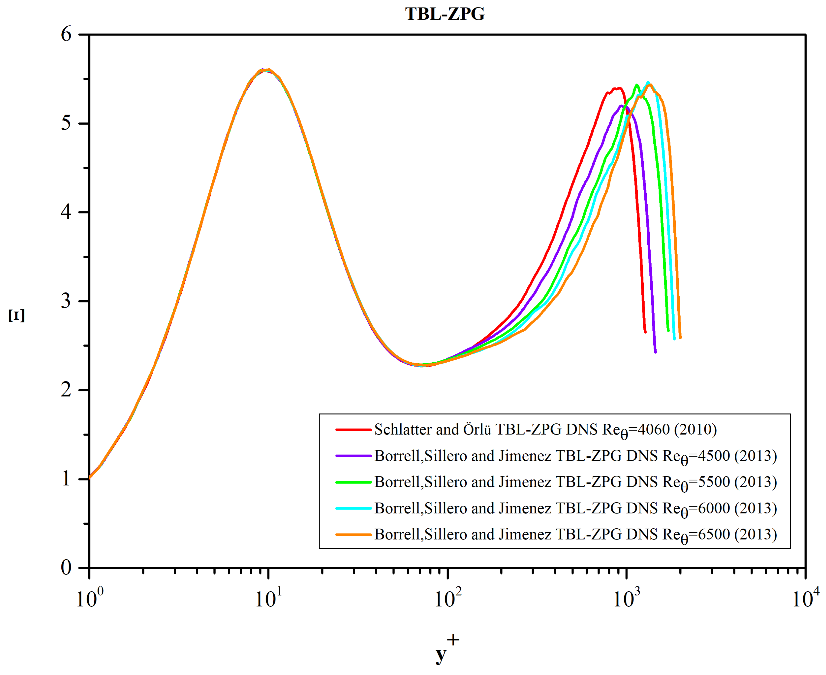
Turning now to the DNS data, per se, we present, in Figure 11, the graphs of function Ξ over the whole boundary layer thickness.
For y+ ≤ 100 all curves collapse on a single curve according to the classical view of an inner law independent of Reθ. Some minor differences appear near the first local maximum of Ξ (“inner peak”) at approximately y+ ≈ 9.5. The magnitude of the inner peak as well as the position where it is located are listed in Table 4. The “inner peak” of Ξ is located within the buffer zone of the MVP and tends to “oscillate” slightly with respect to its mean location (see Table 4).
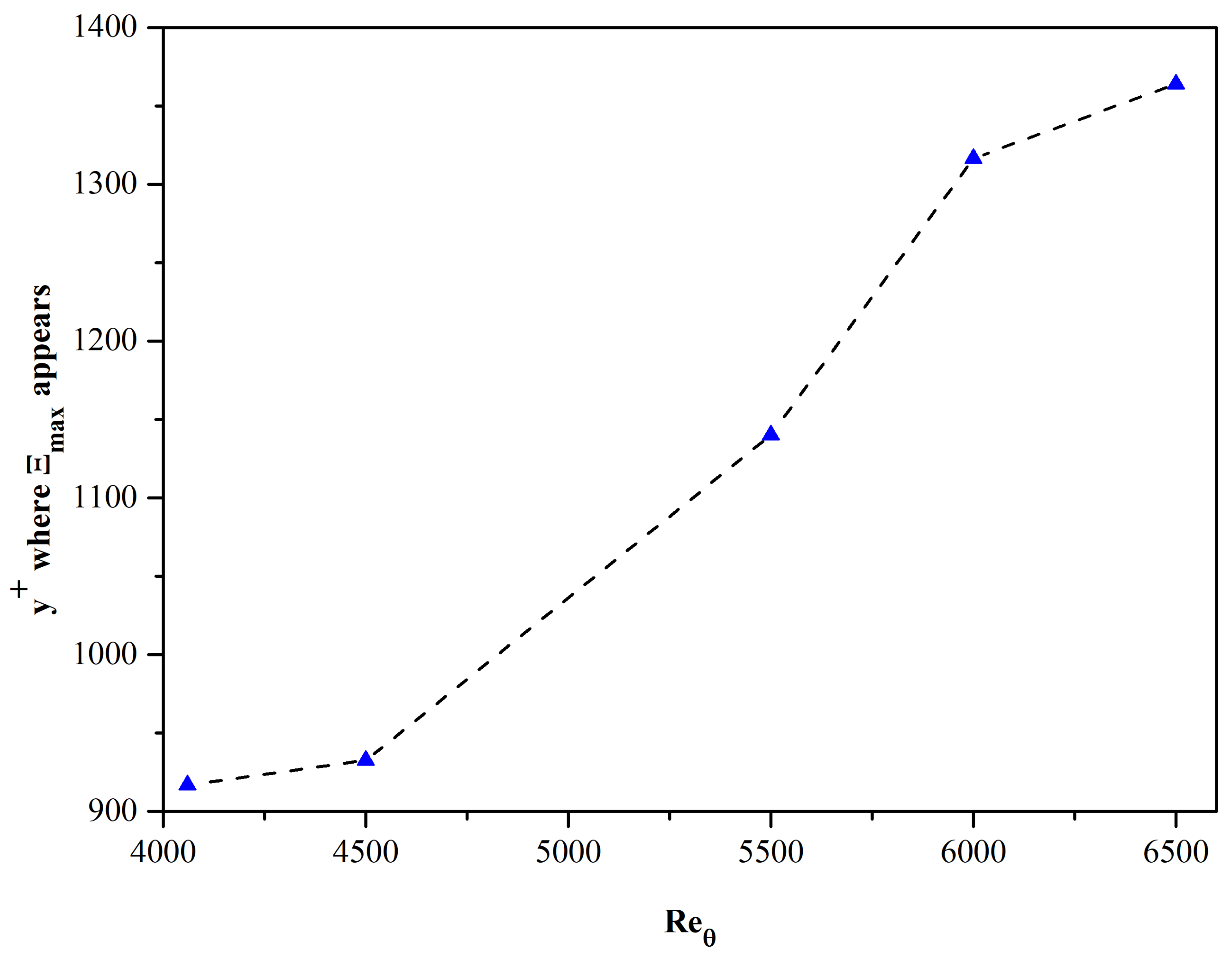
For y+ ≳ 100 the graphs of Ξ separate in accordance with the view that in the outer layer, there are evident Reθ effects on MVPs when plotted in inner law variables. A second local maximum of Ξ (“outer peak”) is formed around y+ ≈ 1150. Table 5 summarizes the “outer peak” values of Ξ as well as the location of the peak for Reθ in the range 4060 to 6500.
The variation in the magnitude of the peak is noticeable. The change in the trend cannot be explained on physical grounds and may maybe an artifact introduced by the different numerical methods used in the case of Reθ = 4060. In addition, the rough character of the computed Ξ in the neighborhood of the “outer peak” may also contribute to the listed values of Ξmax(Reθ). We stress here that no local smoothing of function Ξ was applied. As the momentum Reynolds number increases, the location of the “outer peak” is always shifted towards higher values of y+ (see Figure 12).
Between the inner and outer peaks, function Ξ tends to form an approximate plateau in the interval [60, 250]. This is discussed in Section 4.1.3.
4.1.3. Search for a Logarithmic Layer
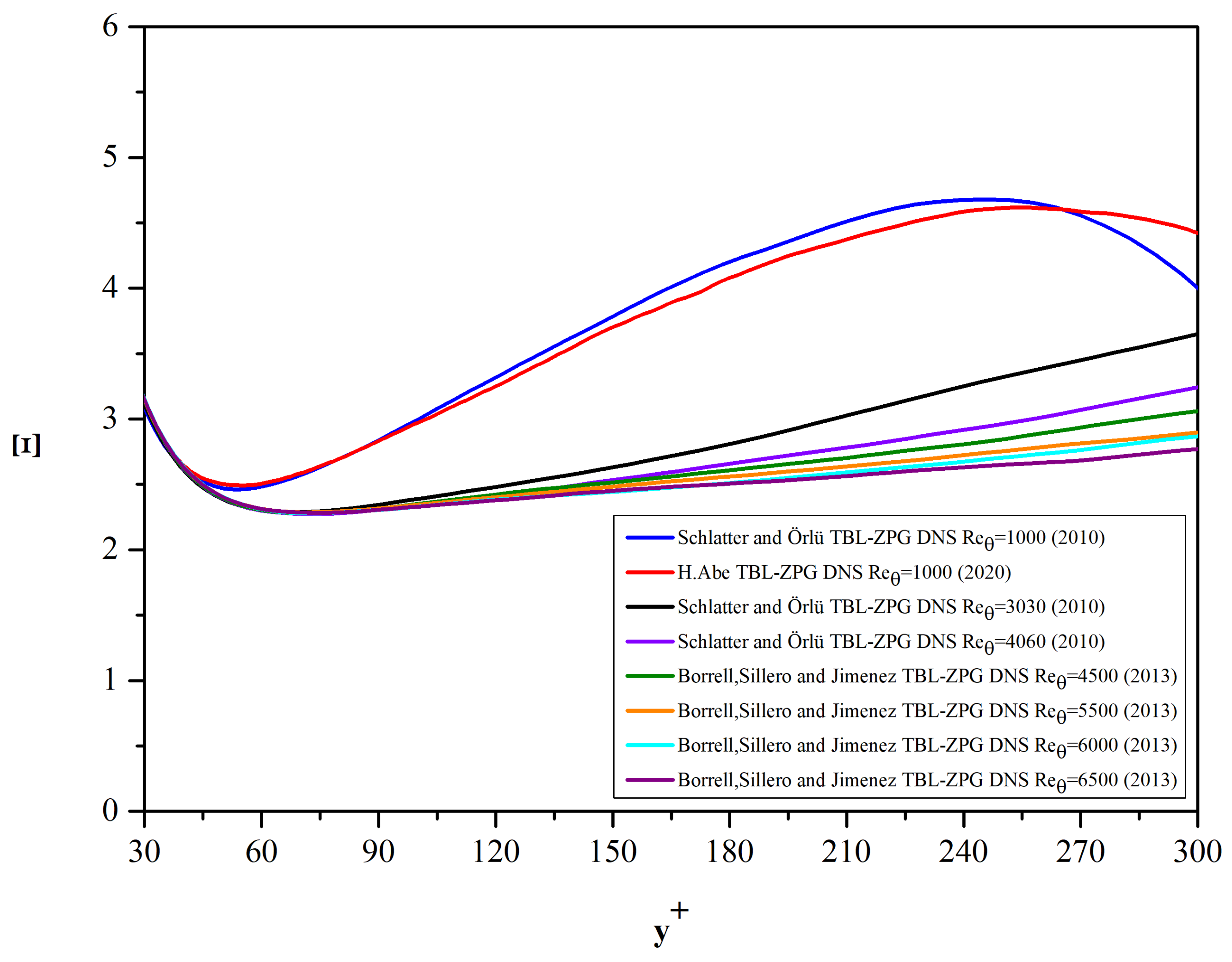
Searching for evidence of a logarithmic layer in the DNS datasets in the range of Reθ [3030, 6500] we focused on the y+ interval [60, 250]. In this interval, a local minimum of Ξ is attained and possibly an approximate plateau is formed. Relevant results are summarized in Table 6 and Figure 13. Based on the data under consideration, it is observed that increasing the Reθ number leads to a larger interval of nearly constant value of Ξ and thus, to a possible determination of the von Kármán’s constant.
In the case of a low Reynolds number, Reθ = 1000, there is a substantial difference in the DNS data of Schlatter and Örlü [13] and Abe [15]. The minimum values, Ξmin, are 2.461 and 2.490 corresponding to estimates of the maximum values of von Kármán’s constant equal to 0.406 and 0.402 respectively. Furthermore, the minimum value of Ξ appears at y+ = 53.3 and y+ = 54.8 respectively (see Table 6). For the DNS data in the range Reθ = 4000 to Reθ = 6500, the minimum value of Ξ appears at y+ ≈ 74. The value of Ξmin shows a remarkable consistency (Ξmin ≈ 2.27) corresponding to a maximum possible value κ ≈ 0.44 for the von Kármán’s constant. This is remarkable since the DNS results of Schlatter and Örlü [13] were obtained by a different numerical method than those of Borrell et al. [14]. However, even for these relatively large values of Reθ, there is no clear evidence of a logarithmic layer (Ξ ≈ const.).
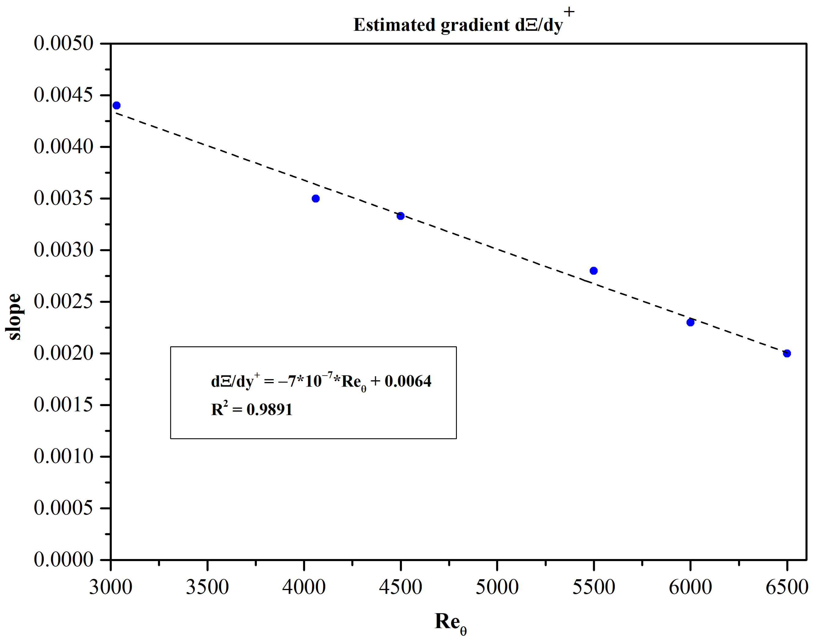
Examining Figure 13 we observe that in the interval [150, 300], as Reθ increases, the slope of function Ξ gradually decreases. This behavior may reflect the initial stages of a process in which the graph of function Ξ reaches gradually a plateau and Ξ converges slowly to a value 1/κ = constant in the limit Reθ → ∞. However, this is a purely speculative remark in view of the limited number of DNS-calculated MVPs published at present and the well—known limitations of DNS in computing flows at high Reθ. The graph of the derivative dΞ/dy+ versus Reθ (Figure 14) shows quantitatively the diminishing slope but reveals nothing with respect to the asymptotic behavior of Ξ as Reθ → ∞.
Laboratory experiments have been designed to study turbulent flows at higher Reynolds numbers but they also face accuracy limitations. Very high Reynolds number laboratory turbulent flows have been achieved mainly in straight pipes [16,17,18,19,20,21,22].
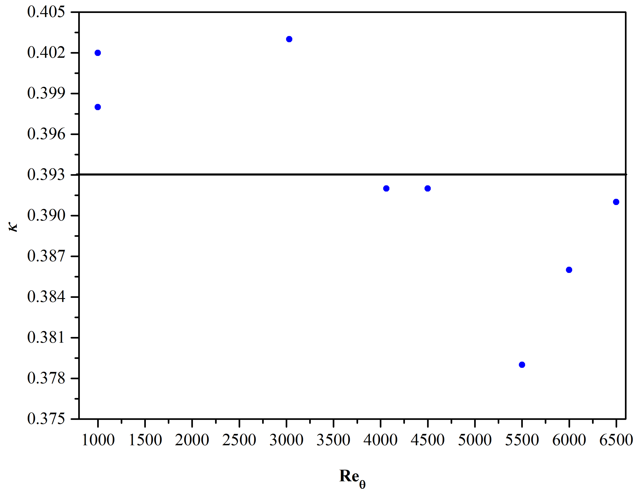
It should be clear to the reader that the approximate estimation of the Kármán constant for the datasets analyzed is to some degree subjective. In contrast, for turbulent flows in channels and pipes, there is overall agreement on upper and lower bounds of the value of Kármán’s constant. Of course, channel and pipe flows are fully developed and unidirectional. On the other hand, turbulent boundary layers are developing flows and the mean flow only approximately may be classified as nearly parallel flow. Even with these limitations in mind, we report on estimates of the Kármán constant (see Table 7).
Assuming that the slopes of the Ξ curves are small enough to be considered negligible, a least—squares—based estimate of a Kármán constant representative in the range 1000 ≤ Reθ ≤ 6500, is found to be equal to κ ≈ 0.393. The dispersion of the data is shown graphically in Figure 15.
A number of attempts have been made by researchers to modify the log-law with mixed results. We mention here, as an example, the effort to use Lie group symmetry methods (e.g., Oberlack [23]) to modify the classical log-law in order to improve the agreement with experimental and DNS data close to the wall. Other researchers attempted to modify the log-wake law (Guo et al. [24]). The discussion of these modifications is beyond the scope of the present work. However, we can state that no proposed modification has been widely and fully accepted by the research community.
4.2. The Diagnostic Function Γ
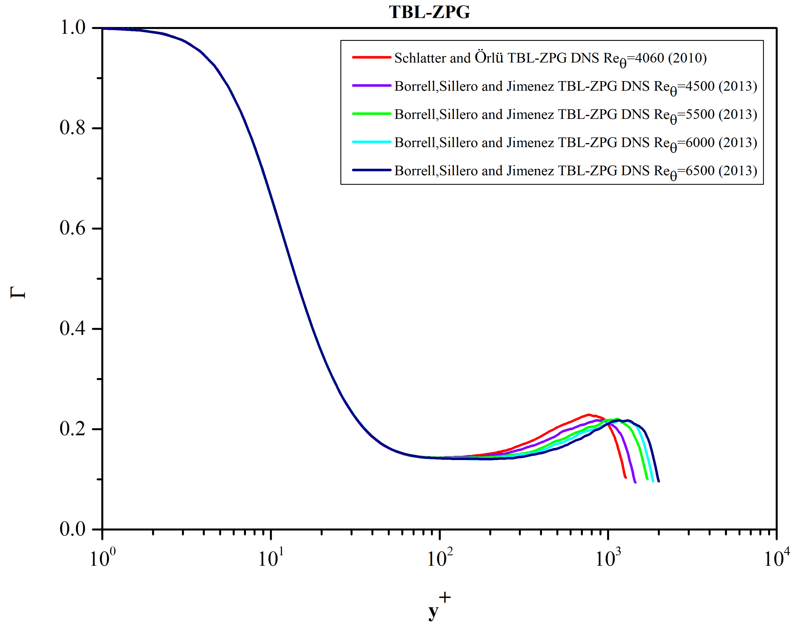
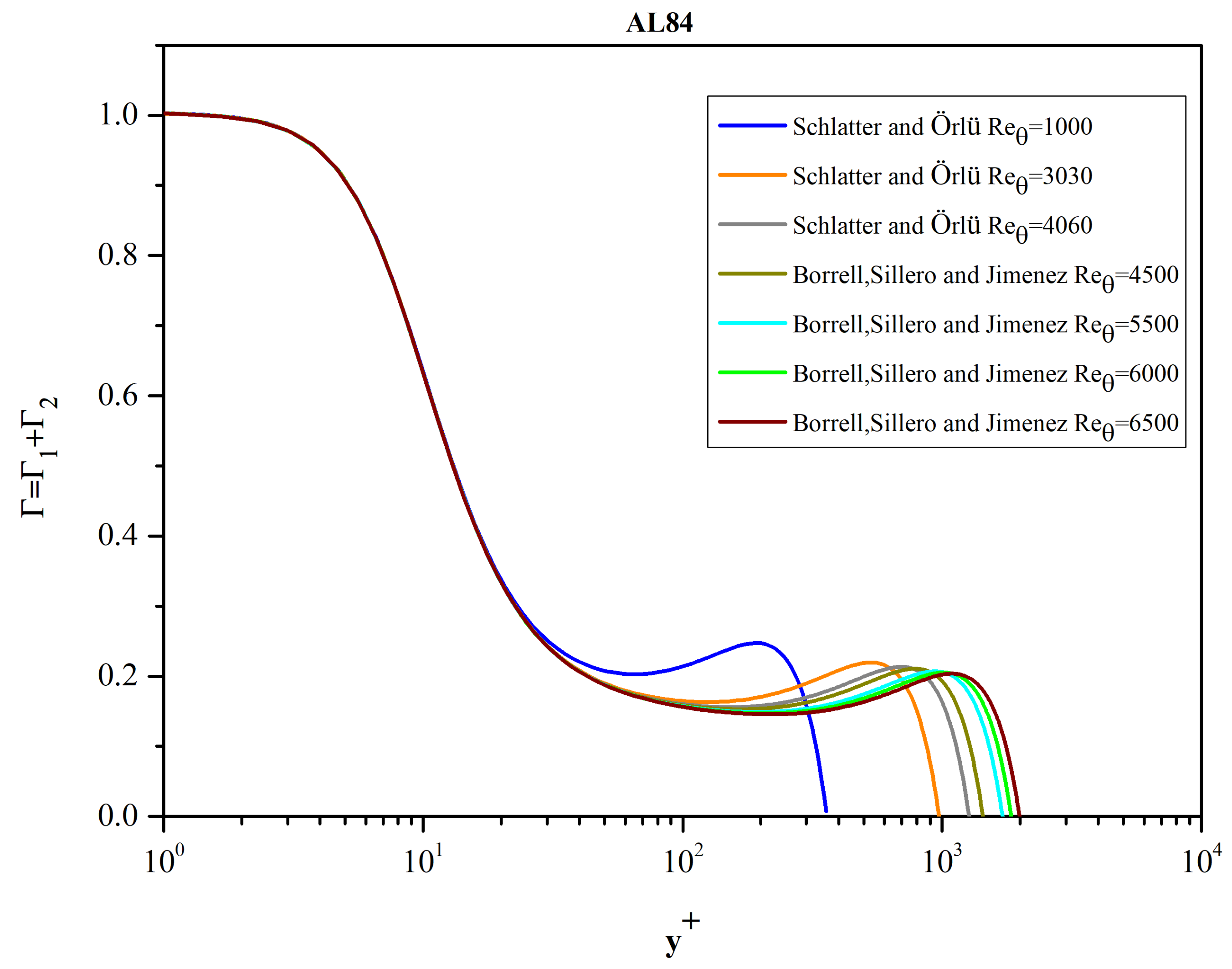
In order to investigate the possibility of a power law approximation in some interval of the MVP, we examine the behavior of the function Γ = over the whole boundary layer thickness. It is straightforward to prove that if a power law of the form u+ = Ay+λ (A and λ constants for a particular value of Reθ) approximates the function u+(y+) in an interval [, ], then Γ attains a constant value equal to λ in that interval.
The diagnostic function Γ, as calculated based on the DNS data, is plotted in Figure 16. In the interval [70, 250], Γ attains a constant value, leading to the estimate λ = 0.145. Another approximate plateau is formed in the interval [800, 1100] for “high” Reynolds numbers, corresponding to an exponent λ = 0.209.
We note that the corresponding predictions of the AL84 model (for high Reθ numbers) are λ = 0.155 for the interval 100 ≤ y+ ≤ 190 and λ ≈ 0.2 = 1/5 for 900 ≤ y+ ≤ 1200 (see Figure 17).
4.3. A Note on the Accuracy of the DNS Profiles
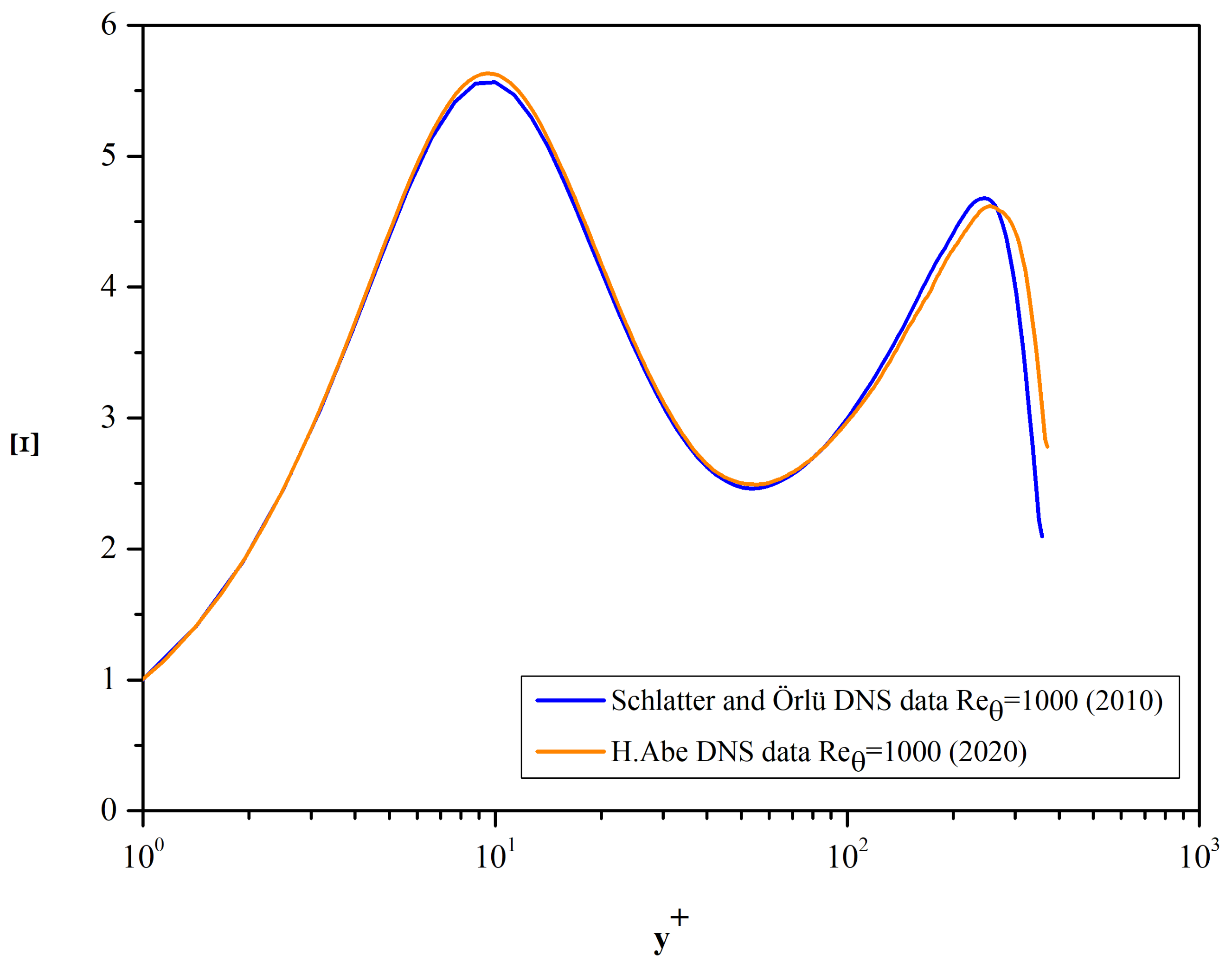
It should be noted that in this paper it was tacitly assumed that the DNS mean velocity profiles (MVPs) were free of errors and they served as the “truth” in comparisons with model AL84. Naturally, this cannot be true. Although the DNS data are of very high quality there are still differences among the profiles computed by various researchers using different numerical methods. For example, in Figure 18 we present the comparison of the Ξ function calculated based on the profiles reported by Schlatter and Örlü [13] and Abe [15] for Reθ = 1000. It is evident that there are some noticeable differences. Comparisons of Ξ(y+) and Γ(y+) present stringent accuracy tests because the numerical differentiation of u+(y+) acts as an error amplifier, and thus, differences between computed MVPs are accentuated.
5. Conclusions
This paper describes the comparison of the AL84 model with high precision and low noise data from direct numerical simulations (DNS) of the zero-pressure-gradient turbulent boundary layer. The influence of the Reθ number on the turbulent velocity profile is analyzed in the range [1000, 6500]. It was deemed useful to divide the presentation into two parts. One concerns the interval where the inner law applies, while in a second stage, the comparison is made over the entire thickness of the boundary layer.
In the first part, the function f(y+) of Equation (4) was used. It was found that there is a very good agreement between the results of the numerical simulation of Schlatter and Örlü [13] and the AL84 model as long as the Reynolds number Reθ is greater than 1000. For y+ ≳ 150, the function f(y+) tends asymptotically to the logarithmic law.
To investigate the velocity profile over the entire thickness of the boundary layer, the function g(Π, ) must be added to the function f(y+). For this purpose, in the second part of the comparison, the use of Equations (2), (4), and (6) is proposed. It turns out that there is agreement between the composite model AL84 and the DNS results, as long as the Reynolds number based on the momentum thickness of the boundary layer is relatively high. When Reθ ≥ 2000, we have very good agreement between the model and the results of the direct numerical simulation of the turbulent boundary layer.
In Section 4 comparisons of the AL84 model with DNS data are presented in terms of the diagnostic functions Ξ and Γ. The analysis of the DNS data per se does not reveal a clear classical logarithmic layer in the range of Reθ studied. The possibility of the formation of a logarithmic layer as Reθ → ∞ is discussed and approximate values for the Kármán constant are estimated for each Reθ analyzed. An overall average value of the Karman constant in the range 1000 ≤ Reθ ≤ 6500 is estimated ≈ 0.39. The power law assumption is better supported by the analysis of the diagnostic function Γ. A clear plateau is formed in the interval 70 ≲ y+ ≲ 250 for 4060 ≤ Reθ ≤ 6500 corresponding to a power law exponent λ = 0.145 = 1/6.89 ≈ 1/7. In comparison for large Reθ the composite AL84 model exhibits a logarithmic behavior with κ ≈ 0.382 in the interval 80 ≲ y+ ≲ 150 and a power law behavior in the interval 100 ≤ y+ ≤ 190 with λ = 0.155.
The AL84 model, as has been verified and validated, is useful in the development and testing of turbulence models valid very close to solid walls [25] as well as in the imposition of boundary conditions near solid surfaces via the wall functions methodology. Furthermore, the explicit form of the AL84 model is very convenient for the imposition of initial conditions in the numerical integration of parabolic Prandtl’s equations for turbulent boundary layers.
Author Contributions
Conceptualization, A.L.; Methodology, A.L.; Software, A.P.; Validation, A.P.; Data curation, A.P.; Writing—original draft, A.L.; Visualization, A.P.; Supervision, A.L.; Funding acquisition, A.L. All authors have read and agreed to the published version of the manuscript.
Funding
This research project was supported by the Hellenic Foundation for Research and Innovation (H.F.R.I.) under the “2nd Call for H.F.R.I. Research Projects to support Faculty Members & Researchers” (Project Number: 4584).
Data Availability Statement
Not applicable.
Conflicts of Interest
The authors declare no conflict of interest.
References
- Bernardini, M.; Pirozzoli, S.; Orlandi, P. Velocity statistics in turbulent channel flow up to Reτ = 4000. J. Fluid Mech. 2014, 742, 171–191. [Google Scholar] [CrossRef]
- Orlandi, P.; Bernardini, M.; Pirozzoli, S. Poiseuille and Couette flows in the transitional and fully turbulent regime. J. Fluid Mech. 2015, 770, 424–441. [Google Scholar] [CrossRef]
- Smits, A.J. Canonical wall-bounded flows: How do they differ? Focus on Fluids. J. Fluid Mech. 2015, 774, 1–4. [Google Scholar] [CrossRef]
- Liakopoulos, A. Explicit representations of the complete velocity profile in a turbulent boundary layer. AIAA J. 1984, 22, 844–846. [Google Scholar] [CrossRef]
- Schlichting, H.; Gersten, K. Boundary-Layer Theory, 9th ed.; Springer Publications: Heidelberg, Germany, 2017. [Google Scholar] [CrossRef]
- Liakopoulos, A. Fluid Mechanics, 2nd ed.; Tziolas Publications: Athens, Greece, 2019. (In Greek) [Google Scholar]
- Coles, D. The law of the wake in the turbulent boundary layer. J. Fluid Mech. 1956, 1, 191–226. Available online: https://authors.library.caltech.edu/38400/1/Coles_1956p191.pdf (accessed on 1 September 2023). [CrossRef]
- Finley, P.J.; Phoe, K.C.; Poh, J. Velocity measurements in a thin turbulent water layer. Houille Blanche 1966, 6, 713–721. [Google Scholar] [CrossRef]
- Granville, P.S. Similarity-Law Characterization Methods for Arbitrary Hydrodynamic Roughnesses; Bethesda: Rockville, MD, USA, 1978; Available online: https://apps.dtic.mil/sti/citations/ADA053563 (accessed on 1 September 2023).
- Dean, R.B. Reynolds number dependence of skin friction and other bulk flow variables in two-dimensional rectangular duct flow. J. Fluids Eng. 1978, 100, 215–223. [Google Scholar] [CrossRef]
- Jones, M.B.; Marusic, I.; Perry, A.E. Evolution and structure of sink-flow turbulent boundary layers. J. Fluid Mech. 2001, 428, 1–27. [Google Scholar] [CrossRef]
- Palasis, A. Turbulent Boundary Layers: Analysis of DNS Data. Diploma Thesis, Department of Civil Engineering, University of Thessaly, Volos, Greece, 31 August 2021. (In Greek). [Google Scholar]
- Schlatter, P.; Örlü, R. Assessment of direct numerical simulation data of turbulent boundary layers. J. Fluid Mech. 2010, 659, 116–126. [Google Scholar] [CrossRef]
- Borrell, G.; Sillero, J.A.; Jiménez, J. A code for direct numerical simulation of turbulent boundary layers at high Reynolds numbers in BG/P supercomputers. Comput. Fluids 2013, 80, 37–43. [Google Scholar] [CrossRef]
- Abe, H. Direct numerical simulation of a non-equilibrium three-dimensional turbulent boundary layer over a flat plate. J. Fluid Mech. 2020, 902, A20. [Google Scholar] [CrossRef]
- Zagarola, M.V.; Smits, A.J. Mean-flow scaling of turbulent pipe flow. J. Fluid Mech. 1998, 373, 33–79. [Google Scholar] [CrossRef]
- McKeon, B.J.; Zagarola, M.V.; Smits, A.J. A new friction factor relationship for fully developed pipe flow. J. Fluid Mech. 2005, 538, 429–443. [Google Scholar] [CrossRef]
- Fiorini, T. Turbulent Pipe Flow-High Resolution Measurements in CICLoPE. Dissertation Thesis, Alma Mater Studiorum Università di Bologna, Bologna, Italy, 4 May 2017. Available online: http://amsdottorato.unibo.it/8158/1/Fiorini_Tommaso_tesi.pdf (accessed on 1 September 2023).
- Marusic, I.; Monty, J.P.; Hultmark, M.; Smits, A.J. On the logarithmic region in wall turbulence. J. Fluid Mech. 2013, 716, R3. [Google Scholar] [CrossRef]
- Smits, A.J.; McKeon, B.J.; Marusic, I. High-Reynolds number wall turbulence. Annu. Rev. Fluid Mech. 2011, 43, 353–375. [Google Scholar] [CrossRef]
- Tschepe, J. On the Prediction of Boundary Layer Quantities at High Reynolds Numbers. Fluids 2022, 7, 114. [Google Scholar] [CrossRef]
- Di Nucci, C.; Absi, R. Comparison of Mean Properties of Turbulent Pipe and Channel Flows at Low-to-Moderate Reynolds Numbers. Fluids 2023, 8, 97. [Google Scholar] [CrossRef]
- Oberlack, M. Asymptotic Expansion, Symmetry Groups, and Invariant Solutions of Laminar and Turbulent Wall-Bounded Flows. ZAMM J. Appl. Math. Mech./Z. Für Angew. Math. Und Mech. Appl. Math. Mech. 2000, 80, 791–800. [Google Scholar] [CrossRef]
- Guo, J.; Julien, P.Y.; Meroney, R.N. Modified log-wake law for zero-pressure-gradient turbulent boundary layers. J. Hydraul. Res. 2005, 43, 421–430. [Google Scholar] [CrossRef]
- Liakopoulos, A. Computation of high speed turbulent boundary-layer flows using the k–ϵ turbulence model. Int. J. Numer. Methods Fluids 1985, 5, 81–97. [Google Scholar] [CrossRef]
Figure 1.
(a) Graphical comparison of Equations (3) and (4). (b) Plot of the difference between Equations (3) and (4).
Figure 1.
(a) Graphical comparison of Equations (3) and (4). (b) Plot of the difference between Equations (3) and (4).

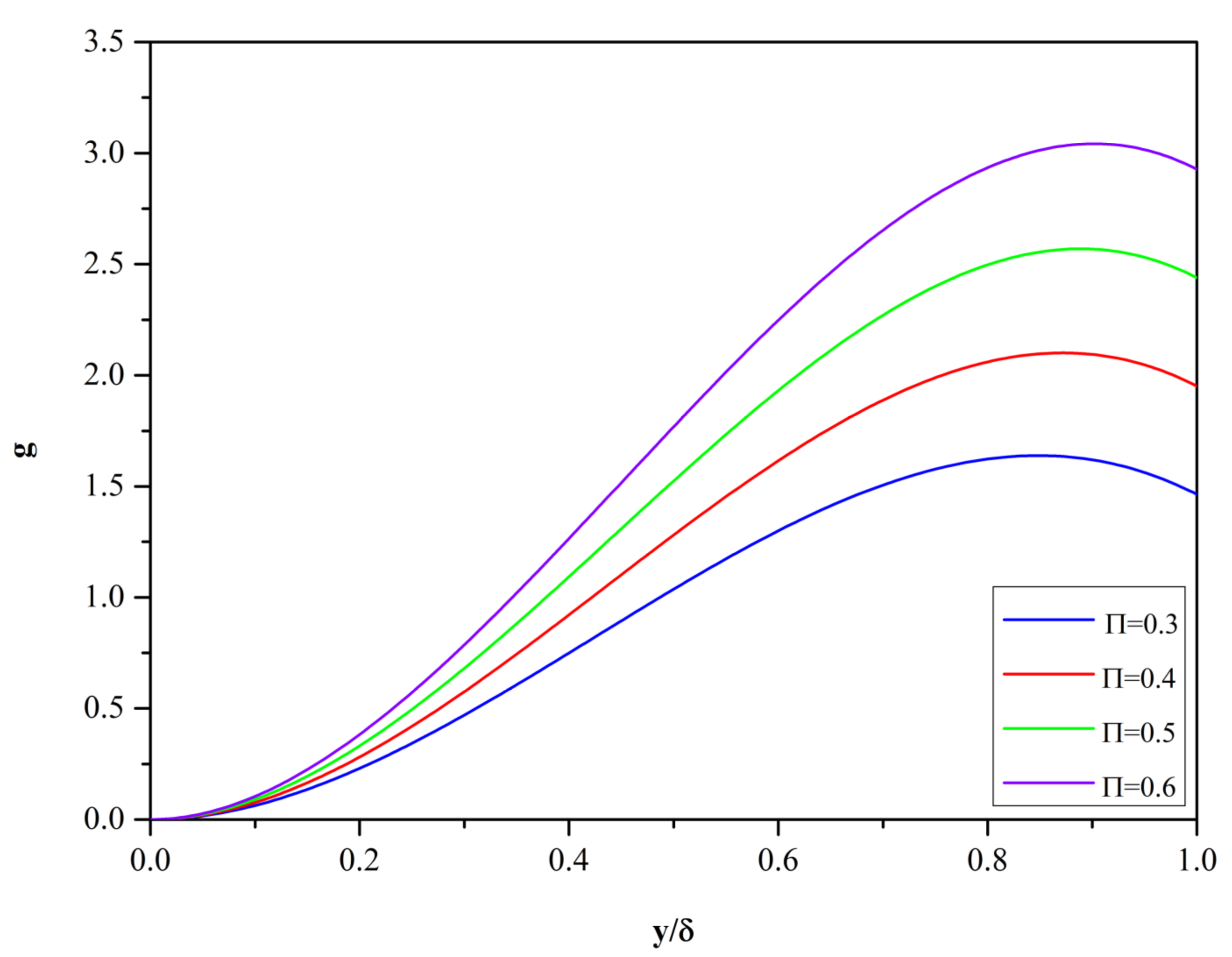
Figure 2.
The function g, Equation (6), for κ = 0.41 and Π = 0.3, 0.4, 0.5 and 0.6.

Figure 3.
Comparison of f(y+) given by Equation (4) with the DNS MVPs of Schlatter and Örlü [13]. Reθ = 1000 (a), 2000 (b), 4060 (c). The deviation from the logarithmic law (for ≥
) points to the need for the inclusion of a wake function.
Figure 3.
Comparison of f(y+) given by Equation (4) with the DNS MVPs of Schlatter and Örlü [13]. Reθ = 1000 (a), 2000 (b), 4060 (c). The deviation from the logarithmic law (for ≥
) points to the need for the inclusion of a wake function.

Figure 4.
Behavior of the difference [u+(y+) − f(y+)] in the inner layer. Reθ = 1000 (a), 3030 (b), 4060 (c).
Figure 4.
Behavior of the difference [u+(y+) − f(y+)] in the inner layer. Reθ = 1000 (a), 3030 (b), 4060 (c).

Figure 5.
Mean velocity profile over the whole boundary layer (0 ≤ y ≤ δ). Comparison of the composite profile, calculated by AL84 model [f + g], and the DNS results reported by Schlatter and Örlü [13] for Reθ = 1000 (a), 2000 (b), 4060 (c). κ = 0.41, Π = 0.55.
Figure 5.
Mean velocity profile over the whole boundary layer (0 ≤ y ≤ δ). Comparison of the composite profile, calculated by AL84 model [f + g], and the DNS results reported by Schlatter and Örlü [13] for Reθ = 1000 (a), 2000 (b), 4060 (c). κ = 0.41, Π = 0.55.

Figure 6.
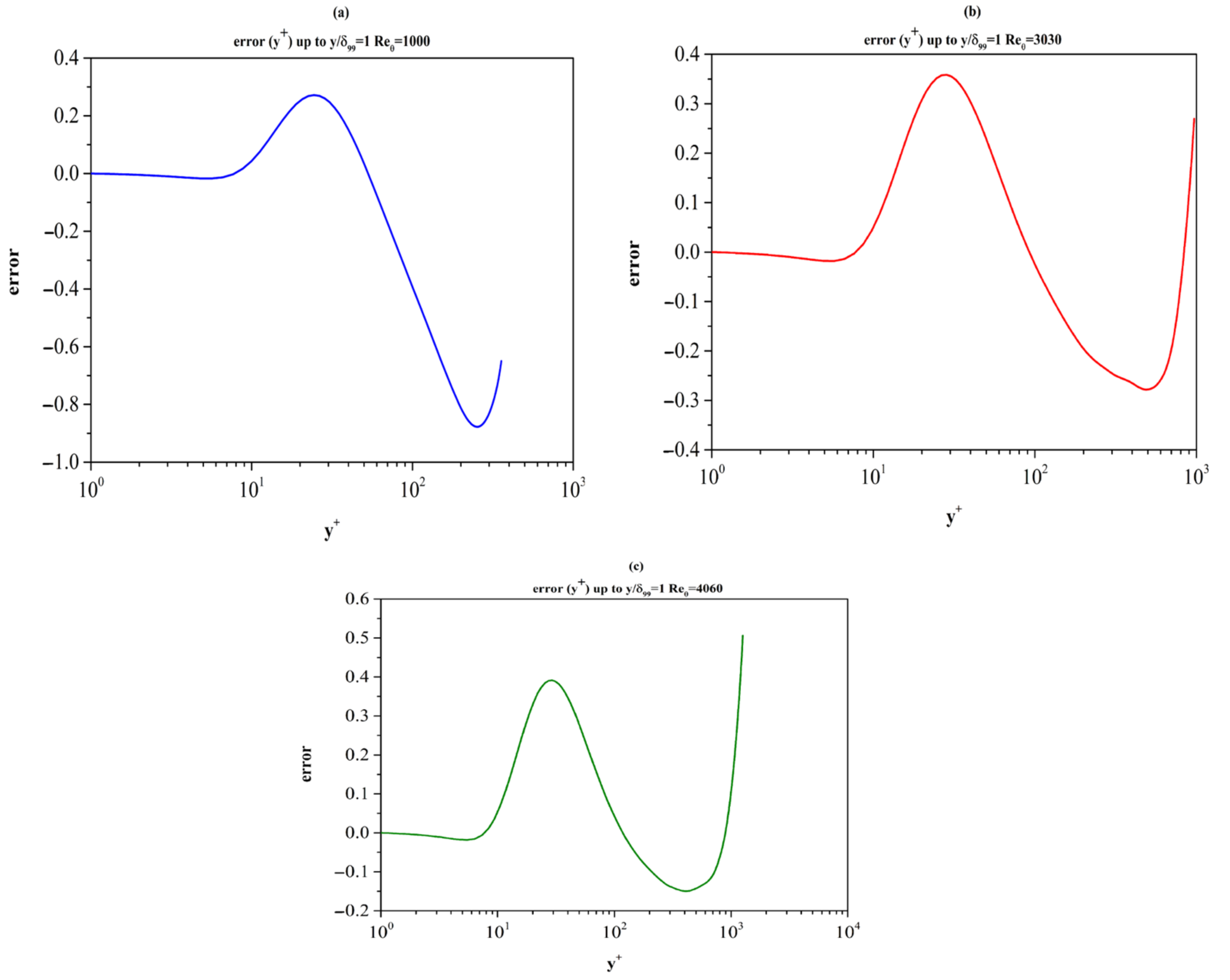
Graphical representation of the error defined as e(y+) = u+(y+) − [f(y+) + g(, Π)] over the entire boundary layer thickness 0 ≤ y ≤ δ. κ = 0.41, Π = 0.55. Reθ = 1000 (a), 3030 (b), 4060 (c).
Figure 6.
Graphical representation of the error defined as e(y+) = u+(y+) − [f(y+) + g(, Π)] over the entire boundary layer thickness 0 ≤ y ≤ δ. κ = 0.41, Π = 0.55. Reθ = 1000 (a), 3030 (b), 4060 (c).

Figure 7.
Schlatter and Örlü [13] data do not exhibit a logarithmic layer for the moderately large Reθ = 4060.
Figure 7.
Schlatter and Örlü [13] data do not exhibit a logarithmic layer for the moderately large Reθ = 4060.

Figure 8.
The function Ξ1 = y+ as predicted by AL84. For y+ ≥ 150 Ξ1 = constant = 2.45.

Figure 9.
The function Ξ2 = y+ as predicted by AL84.

Figure 10.
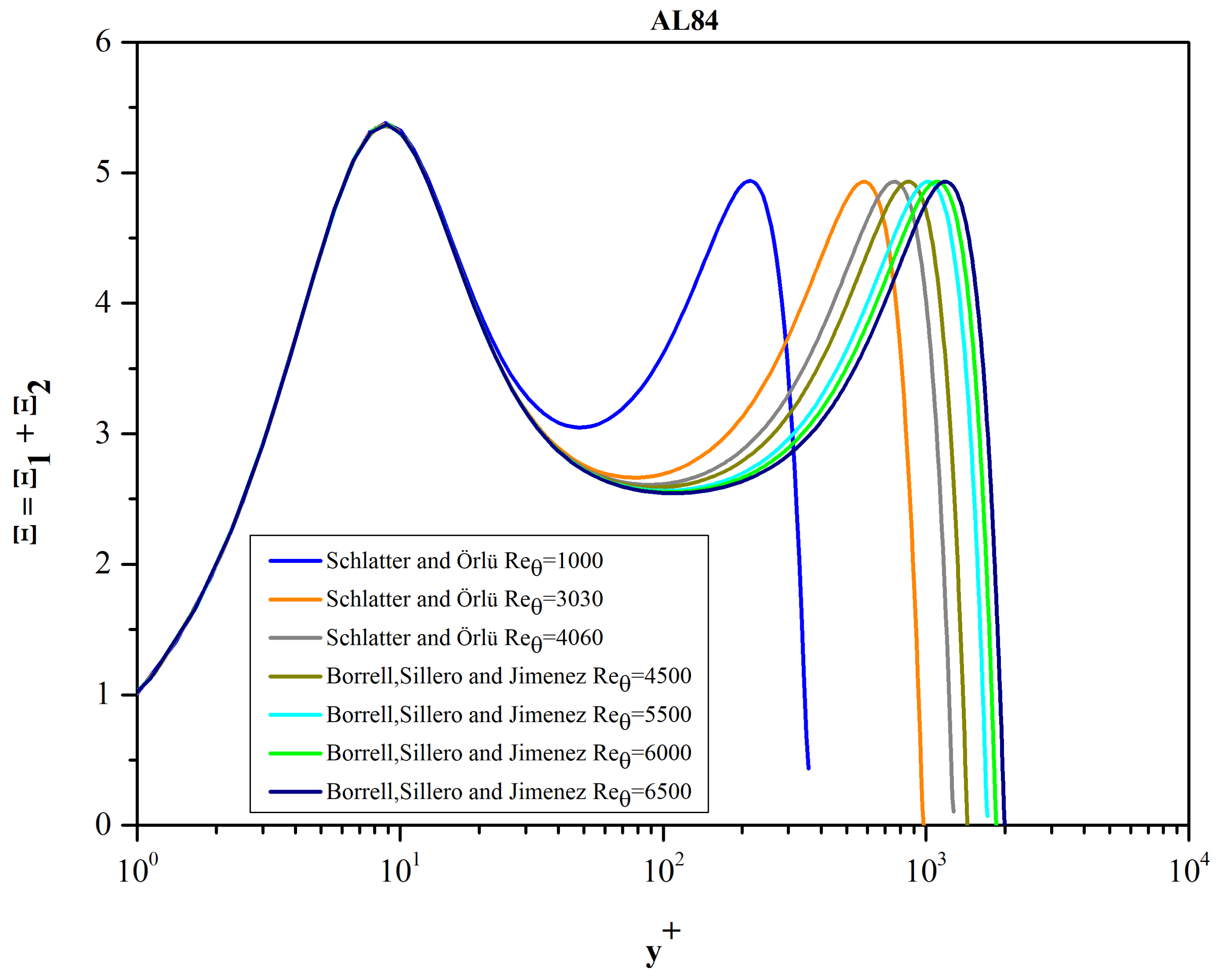
Function Ξ based on the complete AL84 model [f + g].

Figure 11.
Function Ξ based on DNS data.

Figure 12.
Location of “outer peak” of Ξ.

Figure 13.
The behavior of Ξ in the y+ interval [30, 300].

Figure 14.
Blue dots: estimates of the gradient of the diagnostic function for various Reθ. Dotted black straight line: least square fit.
Figure 14.
Blue dots: estimates of the gradient of the diagnostic function for various Reθ. Dotted black straight line: least square fit.

Figure 15.
Upper and lower bounds of the von Kármán’s constant. The black line represents the mean value, κ ≈ 0.393.
Figure 15.
Upper and lower bounds of the von Kármán’s constant. The black line represents the mean value, κ ≈ 0.393.

Figure 16.
Function Γ based solely on DNS data.

Figure 17.
Function Γ based on the complete [f + g] AL84 model. [κ = 0.41, Π = 0.55].

Figure 18.
Differences in Ξ calculated based on Schlatter & Örlü [13] and Abe’s [15] DNS data for Reθ = 1000.


Table 1.
Error quantification in the inner layer.
| Statistics | Reθ = 1000 | Reθ = 3030 | Reθ = 4060 |
|---|---|---|---|
| Mean | 0.1619 | 0.1518 | 0.1727 |
| Standard Error | 0.0162 | 0.0127 | 0.0127 |
| Root Mean Square Error | 0.2011 | 0.1928 | 0.2145 |
| Mean Square Deviation | 0.1205 | 0.1195 | 0.1279 |
| Variance | 0.0145 | 0.0143 | 0.0164 |
| Range | 0.3413 | 0.3849 | 0.4244 |
| Min | −0.015 | −0.0177 | −0.0182 |
| Max | 0.3264 | 0.3673 | 0.4062 |
| Number of data points | 55 | 89 | 102 |
Table 2.
Error quantification in the entire boundary layer thickness 0 ≤ y ≤ δ.
| Statistics | Reθ = 1000 | Reθ = 3030 | Reθ = 4060 |
|---|---|---|---|
| Mean | −0.3399 | −0.0736 | 0.0255 |
| Standard Error | 0.0409 | 0.0143 | 0.0122 |
| Root Mean Square Error | 0.5273 | 0.204 | 0.179 |
| Mean Square Deviation | 0.4053 | 0.1908 | 0.1776 |
| Variance | 0.1643 | 0.0364 | 0.0315 |
| Range | 1.1498 | 0.6367 | 0.6561 |
| Min | −0.8778 | −0.2781 | −0.1496 |
| Max | 0.272 | 0.3586 | 0.5065 |
| Number of data points | 98 | 179 | 212 |
Table 3.
Parameters of DNS MVP profiles and the AL84 model.
| Reference | AL84 Parameters | DNS Parameters | ||||
|---|---|---|---|---|---|---|
| κ | Π | Reθ | Reτ | uτ | θ | |
| Borrell, Sillero and Jimenez, 2013 [14] | 0.41 | 0.55 | 4500 | 1437.066 | 0.0384 | 1.2836 |
| 0.41 | 0.55 | 5500 | 1709.493 | 0.0374 | 1.5691 | |
| 0.41 | 0.55 | 6000 | 1847.654 | 0.0371 | 1.712 | |
| 0.41 | 0.55 | 6500 | 1989.472 | 0.0368 | 1.855 | |
| Reference | AL84 Parameters | DNS Parameters | ||||
| κ | Π | Reθ | Reδ* | Reτ | Cf | |
| Schlatter and Örlü, 2010 [13] | 0.41 | 0.55 | 1000 | 1459.397 | 359.38 | 0.0043 |
| 0.41 | 0.55 | 3030 | 4237.594 | 974.18 | 0.0032 | |
| 0.41 | 0.55 | 4060 | 5633.318 | 1271.54 | 0.003 | |
Table 4.
The inner peak of function Ξ for various DNS datasets: location and value.
| Datasets | Reθ | Position y+ Where Ξmax Appears | Ξmax |
|---|---|---|---|
| Schlatter and Örlü, 2010 [13] | 4060 | 9.427 | 5.599 |
| Borrell, Sillero and Jimenez, 2013 [14] | 4500 | 9.263 | 5.604 |
| Borrell, Sillero and Jimenez, 2013 [14] | 5500 | 9.041 | 5.595 |
| Borrell, Sillero and Jimenez, 2013 [14] | 6000 | 10.225 | 5.598 |
| Borrell, Sillero and Jimenez, 2013 [14] | 6500 | 10.149 | 5.606 |
Table 5.
The outer peak of function Ξ as a function of Reθ: location and value.
| Datasets | Reθ | Position y+ Where Ξmax Appears | Ξmax |
|---|---|---|---|
| Schlatter and Örlü, 2010 [13] | 4060 | 916.807 | 5.397 |
| Borrell, Sillero and Jimenez, 2013 [14] | 4500 | 932.620 | 5.198 |
| Borrell, Sillero and Jimenez, 2013 [14] | 5500 | 1140.034 | 5.433 |
| Borrell, Sillero and Jimenez, 2013 [14] | 6000 | 1316.612 | 5.466 |
| Borrell, Sillero and Jimenez, 2013 [14] | 6500 | 1364.088 | 5.435 |
Table 6.
Local minima of function Ξ in the inner layer. Ξmin values and y+ values where Ξmin appears.
Table 6.
Local minima of function Ξ in the inner layer. Ξmin values and y+ values where Ξmin appears.
| Datasets | Reθ | Position y+ Where Ξmin Appears | Ξmin | “κmax” |
|---|---|---|---|---|
| Schlatter and Örlü, 2010 [13] | 1000 | 53.321 | 2.461 | 0.406 |
| H. Abe, 2020 [15] | 1000 | 54.819 | 2.490 | 0.402 |
| Schlatter and Örlü, 2010 [13] | 4060 | 71.624 | 2.274 | 0.440 |
| Borrell, Sillero and Jimenez, 2013 [14] | 4500 | 69.929 | 2.279 | 0.439 |
| Borrell, Sillero and Jimenez, 2013 [14] | 5500 | 71.351 | 2.287 | 0.437 |
| Borrell, Sillero and Jimenez, 2013 [14] | 6000 | 73.865 | 2.279 | 0.439 |
| Borrell, Sillero and Jimenez, 2013 [14] | 6500 | 73.312 | 2.283 | 0.438 |
Table 7.
Estimates of von Kármán constant for finite Reθ.
| Datasets | Reθ | κ |
|---|---|---|
| Schlatter and Örlü, 2010 [13] | 1000 | 0.402 |
| H. Abe, 2020 [15] | 1000 | 0.398 |
| Schlatter and Örlü, 2010 [13] | 3030 | 0.403 |
| Schlatter and Örlü, 2010 [13] | 4060 | 0.392 |
| Borrell, Sillero and Jimenez, 2013 [14] | 4500 | 0.392 |
| Borrell, Sillero and Jimenez, 2013 [14] | 5500 | 0.379 |
| Borrell, Sillero and Jimenez, 2013 [14] | 6000 | 0.386 |
| Borrell, Sillero and Jimenez, 2013 [14] | 6500 | 0.391 |
Disclaimer/Publisher’s Note: The statements, opinions and data contained in all publications are solely those of the individual author(s) and contributor(s) and not of MDPI and/or the editor(s). MDPI and/or the editor(s) disclaim responsibility for any injury to people or property resulting from any ideas, methods, instructions or products referred to in the content. |
© 2023 by the authors. Licensee MDPI, Basel, Switzerland. This article is an open access article distributed under the terms and conditions of the Creative Commons Attribution (CC BY) license (https://creativecommons.org/licenses/by/4.0/).
Share and Cite
MDPI and ACS Style
Liakopoulos, A.; Palasis, A. On the Composite Velocity Profile in Zero Pressure Gradient Turbulent Boundary Layer: Comparison with DNS Datasets. Fluids 2023, 8, 260. https://doi.org/10.3390/fluids8100260
AMA Style
Liakopoulos A, Palasis A. On the Composite Velocity Profile in Zero Pressure Gradient Turbulent Boundary Layer: Comparison with DNS Datasets. Fluids. 2023; 8(10):260. https://doi.org/10.3390/fluids8100260
Chicago/Turabian StyleLiakopoulos, Antonios, and Apostolos Palasis. 2023. "On the Composite Velocity Profile in Zero Pressure Gradient Turbulent Boundary Layer: Comparison with DNS Datasets" Fluids 8, no. 10: 260. https://doi.org/10.3390/fluids8100260