
Stochastic Modeling of Particle Transport in Confined Geometries: Problems and Peculiarities


Dipartimento di Ingegneria Chimica Materiali Ambiente, La Sapienza Università di Roma, Via Eudossiana 18, 00184 Roma, Italy
*
Author to whom correspondence should be addressed.
Fluids 2022, 7(3), 105; https://doi.org/10.3390/fluids7030105
Submission received: 7 February 2022
/
Revised: 4 March 2022
/
Accepted: 8 March 2022
/
Published: 12 March 2022
(This article belongs to the Special Issue Recent Advances in Single and Multiphase Flows in Microchannels, Volume II)
Abstract
:The equivalence between parabolic transport equations for solute concentrations and stochastic dynamics for solute particle motion represents one of the most fertile correspondences in statistical physics originating from the work by Einstein on Brownian motion. In this article, we analyze the problems and the peculiarities of the stochastic equations of motion in microfluidic confined systems. The presence of solid boundaries leads to tensorial hydrodynamic coefficients (hydrodynamic resistance matrix) that depend also on the particle position. Singularity issues, originating from the non-integrable divergence of the entries of the resistance matrix near a solid no-slip boundary, determine some mass-transport paradoxes whenever surface phenomena, such as surface chemical reactions at the walls, are considered. These problems can be overcome by considering the occurrence of non vanishing slippage. Added-mass effects and the influence of fluid inertia in confined geometries are also briefly addressed.
1. Introduction
The main legacy of the Einsteinian theory of Brownian motion to modern physics lies in the confirmation of the atomistic nature of matter and in the equivalence between random molecular motion at the microscopic level and the macroscopic phenomenon of diffusion [1,2].
Thanks also to the contributions by Langevin, Smoluchowski and many others [3,4,5], it is now common knowledge in applied transport theory [6] that any transport equation, expressed in the form of an advection-diffusion equation for the concentration field of some solute diffusing in a fluid phase,
where is the macroscopic velocity field experienced by the solute (coinciding in most of the applications with the fluid phase velocity ), and D its isotropic diffusivity, can be represented in terms of the microscopic motion of the solute particles by means of a Langevin equation of the form
where is the increment of a three-dimensional Wiener process in the time interval . This equivalence is also computationally important as it enables to solve parabolic transport equations in complex geometries by means of stochastic simulations of the Langevin Equation (2) [7,8,9,10].
The description of physical processes in terms of stochastic Langevin equations, both in equilibrium and in out-of equilibrium conditions, has become one of the strongest and more fruitful research lines in modern statistical physics, providing useful insights in all the fields of physical investigation, including quantum and particle physics [11,12,13].
The Langevin Equation (2), expressed exclusively with respect to the particle position , can be derived from a stochastic dynamics (stochastic Newton equation) of the form
where , , m is the particle mass, the friction factor, T the absolute temperature and the Boltzmann constant, in the limit for , i.e., in the case particle inertia could be neglected. This simplification is not only important in transport theory, but also in the thermodynamics of fluctuations as it implies the simplest form of fluctuation-dissipation relation [14,15],
that, in the case of spherical particles for which ( is the fluid viscosity, the particle radius) is referred to as the Stokes-Einstein relation. Equation (4) connects a transport parameter, related to the intersity of fluctuations (the diffusivity D) to a hydrodynamic quantity, related to dissipation (the friction factor ) at constant temperature T.
The rise of microfludics as an autonomous hydrodynamic discipline has informed recent research in the theory of fluid motion, with relevant practical applications in analytical chemistry, molecular biology and biomedicine, production of high-quality pharmaceuticals, etc. [16,17,18,19]
The analysis of flow systems at microscale in devices (microchannels, microreactors) of almost comparable size than that of solute particles, necessarily implies a more detailed understanding of all the physical processes at small lengthscales, and thus a unitary and integrated use of theoretical tools deriving from practically all the branches of physics coupled to hydrodynamic problems [20]: optical methods for trapping, particle manipulation and detection [21,22] are of common use in microfluidics, and electrosmotic [23,24,25] and acoustic effects [26,27], either for fluid mixing or for separation purposes can be conveniently integrated within a microfluidic device. On the other hand, microscale hydrodynamics represents the natural realm where thermal and hydrodynamic fluctuations play a leading role. This admits also interesting practical implications related to the use of micrometric particles for detecting and measuring superficial phenomena and surface interactions (Brownian probes) [28,29,30]. For 1 m particles, quantum effects and forces become measurable, and this opens the way for testing quantum theories, such as the occurrence of the Casimir effect, using “macroscopic” microfluidic systems [31,32], paving the way for a better understanding of the quantum-to-classical transition.
In most of the microfluidic applications, linearized hydrodynamic equations can be used with reasonable accuracy [33,34]. For timescales much larger than the dissipation time , the instantaneous Stokes equations
where are the velocity, the pressure and the stress tensor of the fluid respectively, provides a good approximation for modeling fluid-particle interactions, and the no-slip boundary conditions at the particle surface ()
where is the velocity and the angular velocity of the particle, and a reference point, say the center of mass of the particle, describe with sufficient accuracy fluid-particle interactions.
Consequently, all the theory of Stokesian hydrodynamics [33,34,35,36], developed throughout more than one and half century, finds in microfluidics a vast field of application. Exceptions to the applicability of the Stokesian hydrodynamics in microfluidics occur for specific inertial effects such as the Segre-Silberberg effect [37,38,39], and the use of “high-Reynolds number flows” (with a Reynolds number order of 100–1000) in microchannels (T- and Y-junctions) for nanoparticle production [40,41,42].
The linearity of the Stokes equations and of the boundary conditions at the fluid-particle interface yields a the linear relation between the velocity of the particle and the hydrodynamic force acting on it, that in the case of a sphere moving in an unbounded fluid consist in the well known Stokes’ laws, and , ( is the force and the torque), where and are scalar coefficients due to the isotropy of the problem and the uniformity of the fluid.
On the other hand, whenever the fluid is confined into a bounded device, corresponding to the hydrodynamic domain bounded by walls, both the symmetries (isotropy and uniformity) are generically broken. Therefore, the hydrodynamic resistance law attains a more general position-dependent and tensorial character
where is the overall resistance matrix of the hydrodynamic interactions, possessing a block structure
where (i) , and are the translational and rotational friction matrices, respectively, (ii) , and are the roto-translational coupling matrices. By the Lorentz’s reciprocal theorem it is possible to prove [33] that and are symmetric matrices, while and satisfy the property , where the superscript “T” indicates the transpose. Correspondingly, the overall resistance matrix is symmetric and positive definite.
This automatically implies, due to the fluctuation-dissipation relation (4), a tensorial and position-dependent diffusivity. The latter two properties have deep and non trivial implications whenever a stochastic equation of motion, in the form of Equation (3) is considered, due to the highly singular nature of the Wiener description of the thermal/hydrodynamic fluctuations. For the sake of completeness, it should be also mentioned that a position dependent effective diffusivity arises in modeling solute transport in microchannels with undulated walls, in the case the transport problem is referred exclusively to the channel axial coordinate [43,44]. This is referred to as the Fick-Jacobs approximation and it is essentially a geometrical effect within an approximate transport model unrelated to any hydrodynamic interactions.
The scope of this article is to analyze in detail the problems and the peculiarities of particle transport in microfluidic systems, originating from the confined nature of the flow, starting from the stochastic description of the microscopic particle motion, in a way that may also be useful for researchers in microfluidics that are not fully familiar with stochastic differential equations. While stochastic modeling of particle transport involving constant effective diffusivities is widely used in the analysis of microfluidic devices, the inclusion of hydrodynamic effects, deriving from fluid confinement, represents a completely new and unexplored field of theoretical and numerical investigation. This article attempts to fill this gap, providing a methodological bridge between hydrodynamic theory and the stochastic formulation of transport phenomena in confined geometries, addressing also in a clear and critical way the complexities and the difficulties of this approach. The article addresses also novel original derivations as regards specific topics, such as the use of the overdamped approximation in non-equilibrium conditions and the effect of slippage as regards transport phenomena involving surface effects (such as surface chemical reactions).
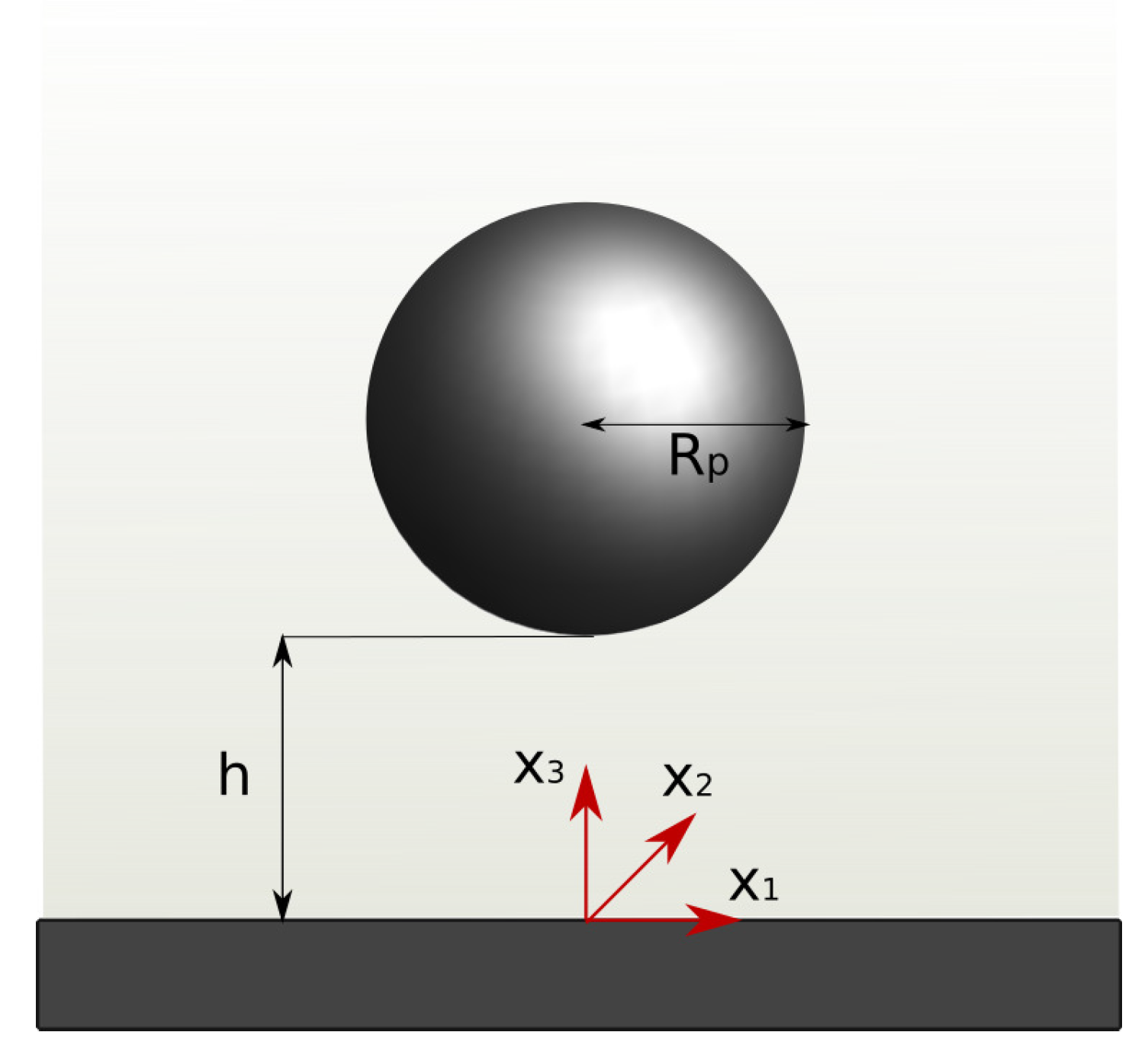
In order to illustrate the physical concepts and the resulting analytical approaches, the hydrodynamics of a spherical particle near an infinite planar solid surface is explicitly considered, as a prototypical and paradigmatic case study of the hydrodynamic problems occurring in microfluidic channels. Throughout this article, rigid particles and Newtonian fluids are considered.
The article is organized as follows. Section 2 addresses the formulation of fluctuation dissipation relations in confined systems, and the computational problems associated with it. Section 3 analyzes the reduction of the equation of motion in the form of a Langevin Equation (3), discussing also the case of non-equilibrium thermal conditions (thermophoresis). Section 4 discusses the problems arising from the non-integrable singularity of the friction factor near a solid no-slip wall, as regards diffusional problems in the presence of superficial phenomena (surface chemical reactions). A way for overcoming these problems lies in relaxing the no-slip assumption, as discussed in Section 5, where we show the necessity of considering slippage effects both at the particle external surface and at the walls of the fluid domain. Finally, Section 6 discusses in a succinct way the role of the fluid inertial effects in the formulation of the stochastic equations for particle motion.
2. Fluctuation-Dissipation Relations in Confined Geometries
Consider the motion of a rigid spherical particle, of mass m and momentum of inertia I, in a microfluidic device. Let and be its velocity and angular velocity, respectively. Assume that the particle is dispersed in a fluid flow, characterized by the fluid velocity and that the particle is also subjected to the action of an external potential field . The particle equations of motion read
where and are the force and the torque deriving from the action of the external flow field (assuming that the particle velocity and angular velocity are vanishing), and are the force and the torque due to the hydrodynamic interactions (described by means of Equation (7) in the case the external flow velocity is vanishing and the particle possesses a velocity and an angular velocity ), and , represent the the stochastic force and the torque deriving from to thermal fluctuations. This decomposition is made possible because the hydrodynamic equations for the fluid are assumed to be linear. The basic problem in the statistical physics of microparticle motion resides in the determination of the contributions of the thermal perturbations and , since all the other terms in Equation (9) stem from a classical hydrodynamic analysis.
Following the original approach due to Einstein and Langevin [15], in the case the fluid is described by means of an instantaneous response (Stoke’s regime), it is natural to represent and in the form of a linear superposition of vector-valued Wiener processes, i.e., as
where and are the increments in the time interval of two mutually independent vector-valued Wiener processes. This observation is a consequence of the fact that Wiener processes are also memoryless, in the meaning that if one defines , interpreted in a distributional meaning, than the correlation function is impulsive (here indicates indifferently either ensemble or temporal averages, and is any time instant) [45].
Henceforth, in order to simplify the notation, the explicit dependence of the matrices on the position will be omitted. While the determination of , and , follows for the simple application of the Stokesian hydrodynamics, the estimate of the matrices entering Equation (10) and defining the thermal perturbations requires a statistical physical ansatz that, at constant temperature T, the thermal fluctuations described by Equation (10) would provide the known result of equilibrium statistical physics [14]. This is the essence of the fluctuation-dissipation ansatz, and for this reason, owing to linearity, it is sufficient to consider the statistical properties for the particle dynamics in the absence of external forcings, i.e., for , . Under these conditions, by substituting Equations (7), (8) and (10) into the equations of motion (9) one obtains,
where also for the explicit dependence on the position has been omitted.
The matrices , , , are the stochastic amplitude matrices, and the final goal of fluctuation-dissipation analysis is their determination from physical principles enforcing equilibrium properties. Let be the overall stochastic amplitude matrix entering Equation (11),
and define the matrix , the entries of which are as
In matrix form,
which is, by definition, symmetric. Expressing Equation (11) componentwise
so that the associated Fokker-Planck equation for the probability density function attains the form [45]
The statistical equilibrium properties can be ascertained from the analysis of the lower-order (first and second) moments of . The first-order moments relax to zero in the long-term regime, as a consequence of the fact that the hydrodynamic interaction matrix is positive definite. It is therefore sufficient to consider the second-order moments for the translational/angular velocities,
To begin with, consider . From the Fokker-Planck Equation (16) one obtains
In the long-term limit (equilibrium), it follows from Equation (18) that
Next, consider , the entries of which satisfy the equations
so that the value attained at equilibrium is
Finally, consider the mixed second-order roto-translational moments
admitting the equilibrium condition
Fluctuation-dissipation conditions, and the explicit expression for the stochastic amplitude matrices follow by enforcing the equilibrium properties [14]
where I is the moment of inertia, and the identity matrix. These conditions stem from the Maxwellian equilibrium velocity distribution, and from the energy equipartition theorem applied to a rigid particle, admitting 6 degrees of freedom. Making use of Equation (24) and of the equilibrium expression Equation (19) for , one obtains that the matrix should be symmetric and
A similar analysis for Equation (21) at equilibrium provides
The equilibrium results deriving from the analysis of the mixed roto-translational moments yield
a solution of which is and
Once the “diffusional” matrices , , , have been expressed in terms of the hydrodynamic resistance matrices, the next step is to derive the expression for the stochastic amplitude matrices , , , .
Because of Equation (28), the matrix defined by Equation (12) is symmetric, and satisfies the algebraic matrix equation
Mutuating this property from the symmetry of hydrodynamic matrices, the matrix is symmetric and positive definite, and it is known from matrix theory [46] that there exists a unique, symmetric, and positive definite matrix solution of Equation (29), formally
In order to determine the explicit expression for the matrix , it is convenient to normalize its entries, expressing the force/torque and the velocity/angular velocity in the same physical dimensions. If is the characteristic particle length, for spherical particle of radius , set , . In this way, has the dimension of a force, and the dimension of a velocity, so that Equations (7) and (8) become
where is the normalized overall resistance matrix possessing the block structure
and the normalized moment of inertia is given by . In this way, Equation (11) attains the normalized representation
with , , , . The normalized matrix Equation (29) thus becomes
and .
For symmetric and positive definite matrices , the estimate of their square root reduces to an eigenvalue problem [46]. Let , , be the eigenvalues of , and the corresponding unit eigenvectors. The solution of Equation (34) can be expressed as
where is the eigenbasis transformation matrix, the column of which are orderly the eigevectors of , i.e.,
and is a diagonal matrix, the diagonal entries of which are the square roots of the eigenvalues , .
An Example: Systems with Axialsymmetric Geometry
As an application of the previous analysis, consider a system with axialsymmetric geometry. Typical axisymmetric systems in microfluidics are spherical particles moving in a slit channel or near an infinitely extended planar wall. The symmetries of the problem reduces the 21 independent coefficients of the hydrodynamic resistance matrix to 5. By taking a Cartesian coordinate system with lying on the axis of symmetry as in Figure 1, the resistance matrix takes the form [33]
Therefore, the matrix , chosing , becomes
where
The eigenvalues of are
where . The eigenvector matrix entering Equation (36) takes in this case the expression
As , i.e., far away from the wall, the coupling term , and the quantity r take the limit form
where
3. Adiabatic Elimination of the Velocity Variables
In this section we consider the formulation of the overdamped approximation for micrometric rigid particles in confined geometries. The overdamped approximation consists in expressing the equations of motion in the form of a kinematic equation for the mechanical degrees of freedom associated with translational and rotational motions. This is made possible due to the fact that velocity variables are customarily characterized by a faster relaxation dynamics than position and orientational variables. This is certainly true for micrometric particles if one considers their transport properties at time scales much larger than the characteristic dissipation timescale , the order of magnitude of which falls between – s for micrometric particles in water at room temperature. For this reason, the overdamped approximation is often referred to as the adiabatic elimination of the fast velocity variables, and this follows by imposing the condition
and extracting out of Equation (49) the expression for and , entering the kinematic equation
where is the vector-valued angular variable accounting for the particle orientation.
The overdamped approximation in confined geometries presents intrinsic peculiarities, just because the hydrodynamic resistance matrix depends on the position , and in general of the orientation , and this raises delicate issues when the thermal fluctuations are expressed as linear superposition of increments of Wiener processes, owing to their highly singular local structure [45]. This problem in the physical literature is usually referred to as the Ito-Stratonovich dilemma [47,48]. The most convenient and simple approach to perform the adiabatic elimination of the fast velocity variable is due to Sancho et al. [49]. The starting point in this derivation is that the configurational coordinates of a particle driven by Wiener fluctuations still represent a locally smooth, and almost everywhere differentiable continuous stochastic process with probability 1, and this property determines the way Equation (49) is interpreted. Without loss of generality, let us suppose that the particle is subjected to an external potential , and that no additional flow contribution are present. The latter can be added at the end of the adiabatic elimination process.
In order to perform this analysis in the simplest formal way, it is convenient to group together configurational and velocity variables, thus introducing the 6-dimensional configurational and velocity variables, and , respectively, and the overall stochastic forcing
so that the equations of motion can be compactly expressed as
where is the mass/moment-of inertial tensor, for a spherical particle, the hydrodynamic resistance matrix, the nabla operator with respect to the -variable and is the matrix of thermal fluctuation intensity satisfying, as discussed in the previous Section, the condition at thermal equilibrium,
The overdamped approximation corresponds to the limit for mass and momentum of inertia tending to zero. In performing this limit, upon correct physical grounds, it should be ensured that the configurational variable is a smooth stochastic process. To this end, the Wong-Zakai theorem can be enforced [50,51], implying that the stochastic differential equation describing particle dynamics should be interpreted in a Stratonovich way [52], Technically, this means that, in performing the limit process, the quantity should be interpreted as
where “∘” indicates the Stratonovich rule in the definition of stochastic integrals and differentials. It is also convenient to recall a known result, deriving from the Ito lemma, namely that [45]
where are the Kronecker’s symbols (entries of the identity matrix), and is a quantity going to zero for faster than .
The final goal of this analysis is to derive a kinematic equation for the configurational particle degrees of freedom (Langevin equation) expressed in the Ito way and, out of it, the transport equation for particle density, corresponding to the Fokker-Planck equation for the statistical characterization of the so-obtained Langevin equation.
Making use of the Wong-Zakai result, expressed by Equation (54), the overdamped approximation of Equation (52) is thus given componentwise by
Expanding the first term at the r.h.s. of Equation (56) in Taylor series to the leading order,
The quantity can be evaluated from Equation (56), by considering for the first term at the r.h.s. of Equation (56) its Ito interpretation, namely that provides the leading order contribution as the remainder in this approximation is order of . Thus, enforcing also Equation (55), one obtains
where , and in deriving the last relation we have made use of Equation (53). Substituting Equations (57) and (58) into Equation (56) it follows that
where the -terms have been neglected. Correspondingly, the Langevin equation in the configuration -space becomes
where
The Fokker-Planck equation for the probability density associated with Equation (61) is thus given by
where and the generalized diffusivity tensor takes the form
i.e., the generalized diffusivity tensor is related to the resistance matrix by the relation
generalizing the fluctuation-dissipation relation Equation (4). Next, consider the contribution of the vector field entering the Fokker-Planck Equation (62). From the identity , it follows componentwise, for any ,
and thus,
The latter expression implies that the entries of defined by Equation (61) reduce to
Substituting Equations (63) and (67) into Equation (62), the Fokker-Planck equation for attains the simpler form
that can be rewritten in a more compact way as
The latter corresponds to an advection-diffusion equation in the configuration space in the presence of the effective velocity , stemming from the potential and of the tensor diffusivity . Conversely, Equation (68) represents the classical formulation of the Fokker-Planck equation associated with a Langevin dynamics interpreted in the Ito way, attaining the following expression
where are the entries of the square root matrix of the diffusivity tensor , . It is also clear from the Ito representation of the Langevin Equation (70) the occurrence of an additional convective contribution depending on the divergence of the diffusivity tensor. This term admits a physical meaning as, even for , it provides a biasing average velocity ,
where is the average value of the particle velocity evaluated when the particle configuration is at [53,54].
In the case of a spherical particle, the hydrodynamic matrices depends solely on and not on . Consequently it is easy to obtain the evolution equation for the marginal distribution , where . Assume also that the spherical particles are immersed in a flow, and that the force exterted by the flow onto a generic particle located at is . In this case, the spatial particle density function satisfies the balance equation
where , is the diffusivity tensor, .
3.1. An Application
As a simple application of the overdamped theory, consider the vertical motion of a spherical particle in the upper half-plane delimited by a planar wall at in isothermal conditions at temperature T. Indicate with the distance of the particle from the wall, and assume that the particle is subjected to an external potential , as in [28,29], where stems from gravity and from a local double-layer repulsive potential near the wall. In this case the problem is spatially one-dimensional, since , and depends solely from the distance x from the wall. Setting , and similarly for , the Fokker-Planck equation for the density function reads
and this equation corresponds to the Langevin-Ito equation
where is the increment of a one-dimensional Wiener process. Assuming that the potential is attractive towards at large distances, so that , it follows from Equation (73) that in the limit for , the density converges towards a stationary density , solution of the equation
corresponding, as expected, to the Boltzmann distribution
This is a classical result, starting from which, micrometric particles may be used as Brownian probes, upon recording their statistical properties i.e. their stationary density function , in order to investigate and measure surface properties of materials [28,29].
It is instructive to analyze in greater detail the mathematical properties of Equation (73). This is a one-dimensional parabolic equation for , and as the wall at is impermeable to particle transport, for any . To solve Equation (73), it should be equipped with initial and boundary conditions. As regards the initial condition, , with . The boundary condition at infinity, is the classical regularity condition, namely
meaning that and should decay faster than any power of x for . At , the zero-flux boundary condition applies, implying in the present case
Two cases should be discussed. If, (i) , since , the wall boundary condition at blows up, reducing Equation (78) to a trivial identity that does not provide any condition on the local behavior of near . Conversely, if (ii) , and moreover , where the constant C may even diverge to ∞, the boundary condition (78) reduces to a homogeneous Dirichlet condition,
As in principle, the condition on the potential U leading to Equation (79) could not be verified in a physical systems, as for the case analyzed in [28,29], it follows from the above analysis that the simple transport model Equation (73) displays a singular behavior as regards the wall boundary conditions. This singular phenomenon is a peculiar feature of the transport equations involving a hydrodynamic Stokesian description of the fluid-particle interactions in confined geometries, deriving from the singularity of some entries of the resistance matrix near a solid wall.
3.2. Thermophoresis from the Overdamped Approximation
An interesting byproduct of the overdamped analysis discussed above is the derivation of thermophoretic effects from the stochastic equations of motion. For simplicity, let us consider the case of a spherical particle in its translational motion, neglecting rotational effects and in the absence of any external or fluid forcing. It has been shown in [55] (see also [56]) that even in the presence of a non-equilibrium steady temperature profile the fluctuation-dissipation relation can be applied, so that the equations of motion in the present case read
Within the overdamped approximation, enforcing the same Stratonovich-approach developed in Section 2 to the term , one obtains
Since,
This leads to the following Langevin equation
From the fluctuation-dissipation relation extended to non-equilibrium steady thermal conditions, , it follows, for any , that
which implies
From the latter expression it follows that
Therefore, Equation (82) becomes
and the corresponding Fokker-Planck equations reads
providing the occurrence of an additional convective contribution to the flux, depending on the temperature gradient, and equal to
providing a thermophoretic velocity equal to [57]. This result shows that thermophoretic effects naturally follow from the accurate description of stochastic particle motion in thermal non-equilibrium conditions.
4. Wall Singularities: Superficial Phenomena
In the previous Section we have outlined the physical problems associated with the setting of boundary conditions for transport equations in confined geometries due to the singularities of the entries of the resistance matrix. The asymptotic trends of all the entries of of two smooth no-slip surfaces almost in contact, such as the case of a particle very close to a solid surface, has been studied by Cox [58] for any value of the walls’ curvatures. From the Cox’s analysis, it results that the drag force on a particle moving towards the wall is inversely proportional to gap between the surfaces (particle and wall surfaces). To simplify the analysis, let us focus on a spherical particle of radius . By considering a Cartesian reference system with the origin on the wall and with colinear to the axis passing between the two contact points of the two surfaces, we have that as . For example, the drag force on a sphere moving towards a planar wall can be expressed to the leading order by the Taylor approximation [59]
for small gaps h between sphere and planar wall. At larger distances, Lorentz [60] found
and, since , a reasonable approximation over the whole range of h values is given by
The singularity of at the wall implies that a particle, initially at and moving towards the solid surface due to the action of a constant force , say gravity, reaches the surface in an infinity time , being the integral
divergent to infinity. The characteristic time is referred to as the wall touching time. This result poses severe problems in predicting the kinetics of coalescence and deposition of dispersed particles from hydrodynamic theories based on the Stokes model Equation (5). To complete the picture, let us consider the scaling behavior of the remaining resistance coefficients. As regards the other coefficients, they are all logarithmically singular as with the exception of the rotational resistance around the normal axis to the surfaces attaining a finite value close to the wall, i.e., as . Singularities at a contact point between surfaces are typical of Stoke’s flows due to the no-slip conditions at solid boundaries. For example, in contact line motions [61] and for flows near a corner [62] it has be found that unphysical singularities can be eliminated or mollified by introducing slippage at solid boundaries [63,64]. Before, addressing the effect of slip boundary conditions, it is useful to investigate further the pathologies arising from the classical no-slip hydrodynamic description in dealing with surface phenomena.
Surface Phenomena and Hydrodynamic Singularities
All the surface phenomena (particle coalescence, surface aggregation, adsorption, surface chemical reactions) depending on a transfer mechanism of molecules and particles from the fluid phase onto the surface are deeply influenced by the spatial dependence of the entries of the hydrodynamic resistance matrix. Paradoxes arise due to the singularities of these entries at the solid walls (for incompressible flows, assuming no-slip boundary conditions at the solid boundaries).
In order to highlight these phenomena, it is sufficient to consider a simple problem, namely the pure diffusional motion of solute particles (nanoparticles) in the neighborhood of a solid wall (located at ), undergoing at the solid wall a surface chemical reaction characterized by a linear, first-order kinetics. To simplify the analysis, let us assume that far away from the wall, say at , the particle concentration is kept fixed, and equal to . The problem is thus specified by the parabolic diffusion equation for the particle concentration ,
equipped with the boundary conditions
Consider the steady-state solution of Equation (94). From Equation (94) it follows that,
where B is a constant, and thus
where A is a second constant to be determined from the boundary conditions. From Equation (97) it follows that a solution exists provided that is locally integrable near . But this is not the case when the hydrodynamic modeling deriving from incompressible Stokes equations imposing no-slip boundary conditions at the solid walls, as .
On the other hand, in the case would be locally integrable near , the steady-state solution would attain the expression
It is clear from the above problem that Stokes’ hydrodynamics applied to transport phenomena coupled to any form of superficial chemical physical processes determines unphysical paradoxes. In the present case, the paradox can be resolved within a classical hydrodynamic formulation by deriving, from more general hydrodynamic conditions, a diffusion coefficient that is integrable near , i.e., such that , with and . Indeed, this property can be recovered by relaxing the no-slip boundary conditions as addressed in the next Section.
5. Effect of Slip Boundary Conditions
Although the no-slip assumption, , at the interface between a Newtonian fluid and a solid boundary is largely accepted due to its capability of predicting mechanical and hydrodynamical properties involving macroscopic bodies and large-scale systems, the nature of the proper boundary conditions for the tangential velocity at a solid interface has been a long-debated issue over more than two centuries of hydrodynamic research [65]. As an alternative to the no-slip hypothesis, Navier [66] proposed that the tangential stresses at any point on the solid surface should be the same as the stresses at a neighboring internal point of the fluid, providing the boundary condition
where is the identity matrix, , the unit normal vector to the surface of the solid, a friction constant and “⊗” indicates dyadic composition, . Since the isotropic pressure contribution entering vanishes at the r.h.s of Equation (99), the Navier’s boundary condition (99) can be written as
where , having the dimension of a length, is the so called slip length. It is evident that the slip length represents a new parameter in modeling Stokes flow. In fact, while the no-slip model describes an idealized fluid/solid interface, the slip model introduces an additional parameter related to the chemical physical interactions at the solid-liquid interface.
Slip phenomena can be distinguished in two main classes: intrinsic slip and apparent slip [67]. The first one is due exclusively to the molecular dynamics at the solid-liquid interface. The second one is due to artifacts at the surfaces that can increase or decrease the slippage, such as the presence of gas bubbles or the surface roughness. However, these artifacts have necessarily a characteristic length below which no-slip conditions applies. In addition, as shown by Cox [58], the nature of the singularity does not depend on the curvature of the approaching surfaces. In considering very small gaps between the surfaces (), the apparent slip vanishes. Therefore, in the remainder, we will refer solely to the intrinsic (molecular) slip. The occurrence of slippage depends in principle, either on hydrodynamic conditions or on the gap length. In fact, as shown by molecular dynamic simulations [68], the slip length for the system (PA-6,6 oligomer)-graphene increases by increasing the shear rate and by reducing the gap between the solid walls. Being such behavior, due to the molecular rearrangement of the fluid, it is appreciable solely when the gap is small enough to be comparable with the characteristic size of the molecular structure of the fluid. However, at this lengthscale scale, it is not possible to mark a clear distinction between the solid surface and the domain of the fluid used in continuous hydrodynamic models, due to solvation and diffusive phenomena. Therefore, a constant slip length, used in hydrodynamic theories (and in the remainder), should be considered as a parameter emerging from the complexity of the molecular system. A review of typical slip lengths for several fluid-surface systems obtained experimentally is given in [67]. Non vanishing values of the slip length are in the range nm, whereas typical characteristic lengthscales of colloids are nm. Correspondingly, the dimensionless slip length for a colloid attains values in the range .
Owing to the linearity of the slip boundary conditions Equation (100), a linear relation between resistance and particle velocity Equation (7) still holds. In [33], a purely mechanical proof of the symmetry of the resistance matrix has been provided, alternative to the thermodynamic approach followed in [69]. However, this proof, as opposed to the thermodynamic one, considers solely no-slip conditions at the solid surfaces. To fill this gap, Appendix A provides a more general proof of the symmetry of the resistance matrix also in the presence of slippage enforcing mechanical arguments.
Either the problems of translating or rotating sphere in an unbounded fluid have been solved by Basset [70] in the presence of the Navier’s slip obtaining the following expressions for the force and the torque acting on the sphere
Being , larger spherical particles experience the force and the torque corresponding to no-slip boundary conditions and , whereas for smaller colloids the Basset’s correction becomes necessary.
For a particle in a confined geometry, the slip boundary conditions can be considered either at the surface of the particle (), with a slip length , or at the surface of the walls () with a slip length . Therefore, the boundary conditions for the flow become
Spherical Particle Moving Perpendicular to a Planar Wall
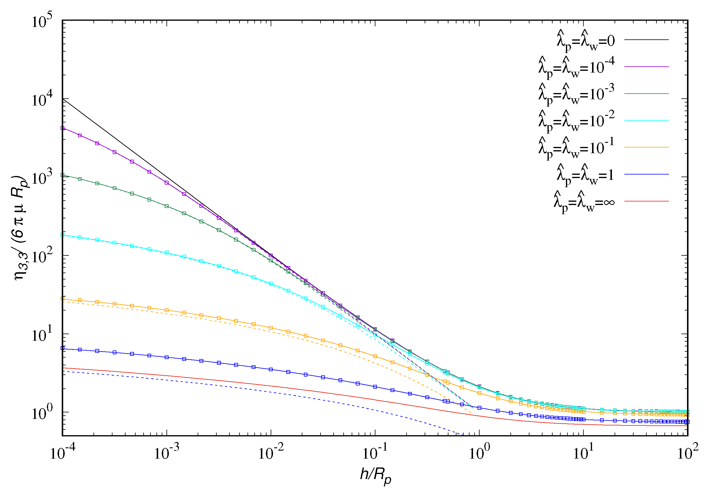
Let us to consider the problem of a spherical particle near a planar wall as depicted in Figure 1. Hocking has shown [71] that, in the presence of the same slip on both the surfaces (), the touching time in Equation (93) becomes finite although the singularity of the transversal resistance at the wall still remains [71]. The functional dependence of the resistance to perpendicular translations on h in the limit , derived by Hocking using lubrication methods, attains the form
where . Consequently, the drag force is logarithmically singular at the wall, Equation (91) becomes integrable and the touching time attains a finite value.
A seminalytical expression for the drag force over a sphere translating perpendicularly to a plane has been obtained by Goren [72] over the entire range of positions and for any values of and using a bispherical coordinate system. However, the author [72] has provided only few numerical values for corresponding to relatively large gaps and slip lengths, and considering solely the case . In point of fact, in order to obtain the numeric values for the transversal resistance from the Goren’s solution is in principle necessary to solve an infinite dimensional linear system of equations for any position of the sphere. On the other hand, the infinite linear system, truncated to a finite number N of equations, provides approximate but accurate values for the force experienced by the particle with an error that decreases as N increases, while the number of the equations from a fixed accuracy increases as and the slip lengths increase.
In order to obtain the values of for different slip lengths and at any distance from the wall, we have either performed FEM simulations, the detail of which are reported in the Appendix B, or solved the Goren’s equations up to . The data depicted in Figure 2 show that the Hocking asymptotic Equation (104) matches accurately the FEM simulations and the Goren solution in the range of and that the predicted logarithmic scaling starts to appear for gaps smaller then the slip length (), after a transition zone, where .
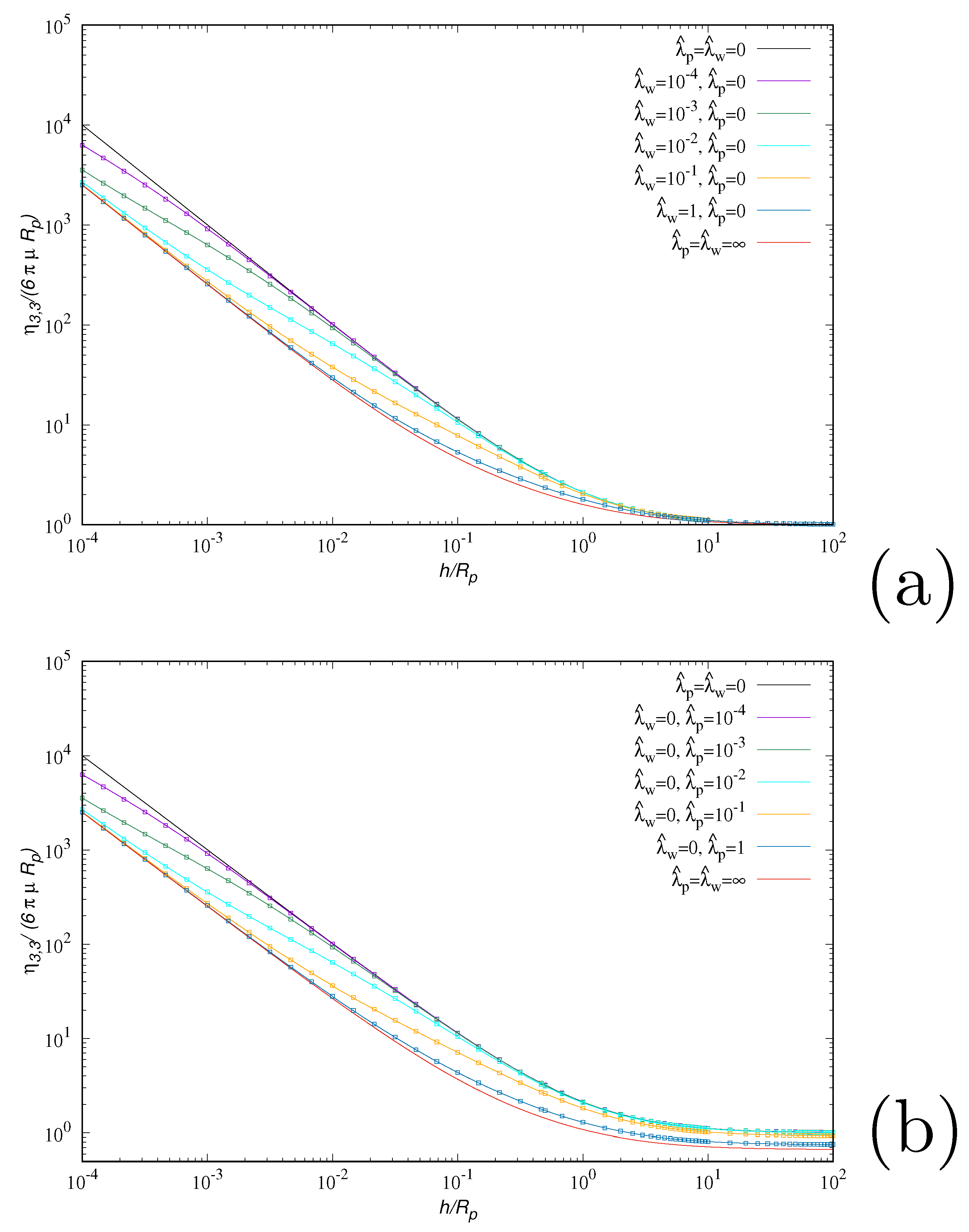
On the other hand, as depicted in Figure 3, if the no-slip boundary condition is imposed on solely one of the surfaces, the singular scaling remains no matter the value of the slip length imposed on the other surface. In the latter conditions, we can distinguish three different regimes: (i) the scaling for , (ii) an apparent logarithmic behavior for and (iii) the asymptotic regime where for .
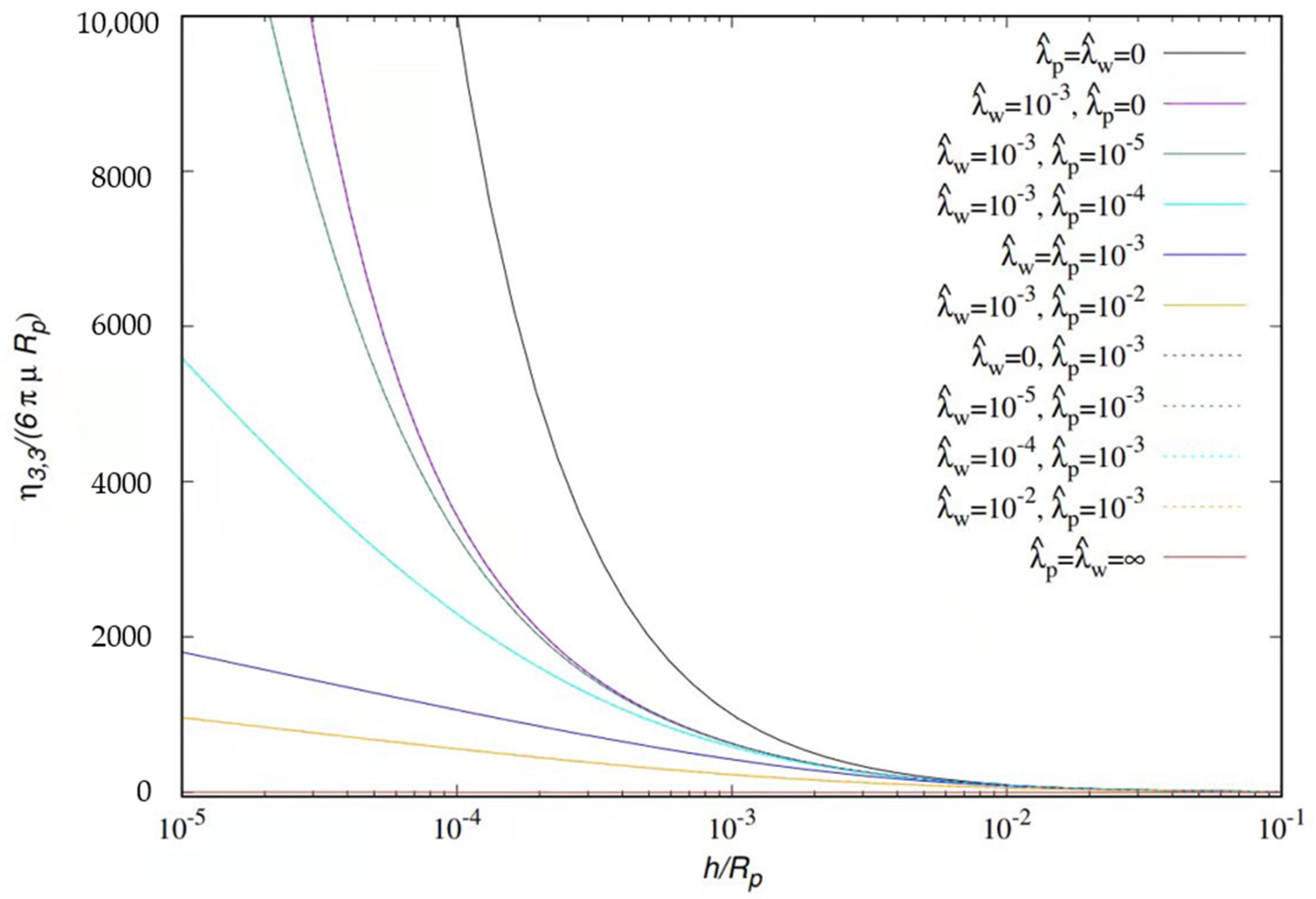
To complete the analysis the data in Figure 4 show that, keeping fixed the slip length at one of the surfaces (, ) and increasing the slip length on the other , , the logarithmic scaling occurs for . This means that an arbirarily small slip on both the surfaces is sufficient to determine an asymptotic logarithmic scaling of the transversal resistance and thus the occurrence of a finite value of the touching time.
6. Fluid Inertial Effects
So far we have considered fluid-particle interaction within the instantaneous Stokes regime, neglecting fluid inertia. In point of fact, while the Reynolds number is smaller that 1 in most of the microfluidic applications, this is not the case of the product of the Reynolds number times the Strouhal number, which is order of 1 or higher due to the high frequency of the thermal fluctuations. This means that a more accurate description of particle motion at short time and length scales would involve a hydrodynamic description of fluid inertia, which in the present case corresponds to the time-dependent Stokes regime [69],
with .
It is well known that the force exerted by a fluid with density and viscosity on a spherical particle of radius moving with velocity in a still fluid, can be expressed in the Laplace domain as [34]
The first term at the r.h.s of Equation (106) is the Stokesian friction factor, the second one corresponds in the time domain to the convolutional Basset force
and the third term is the added-mass contribution
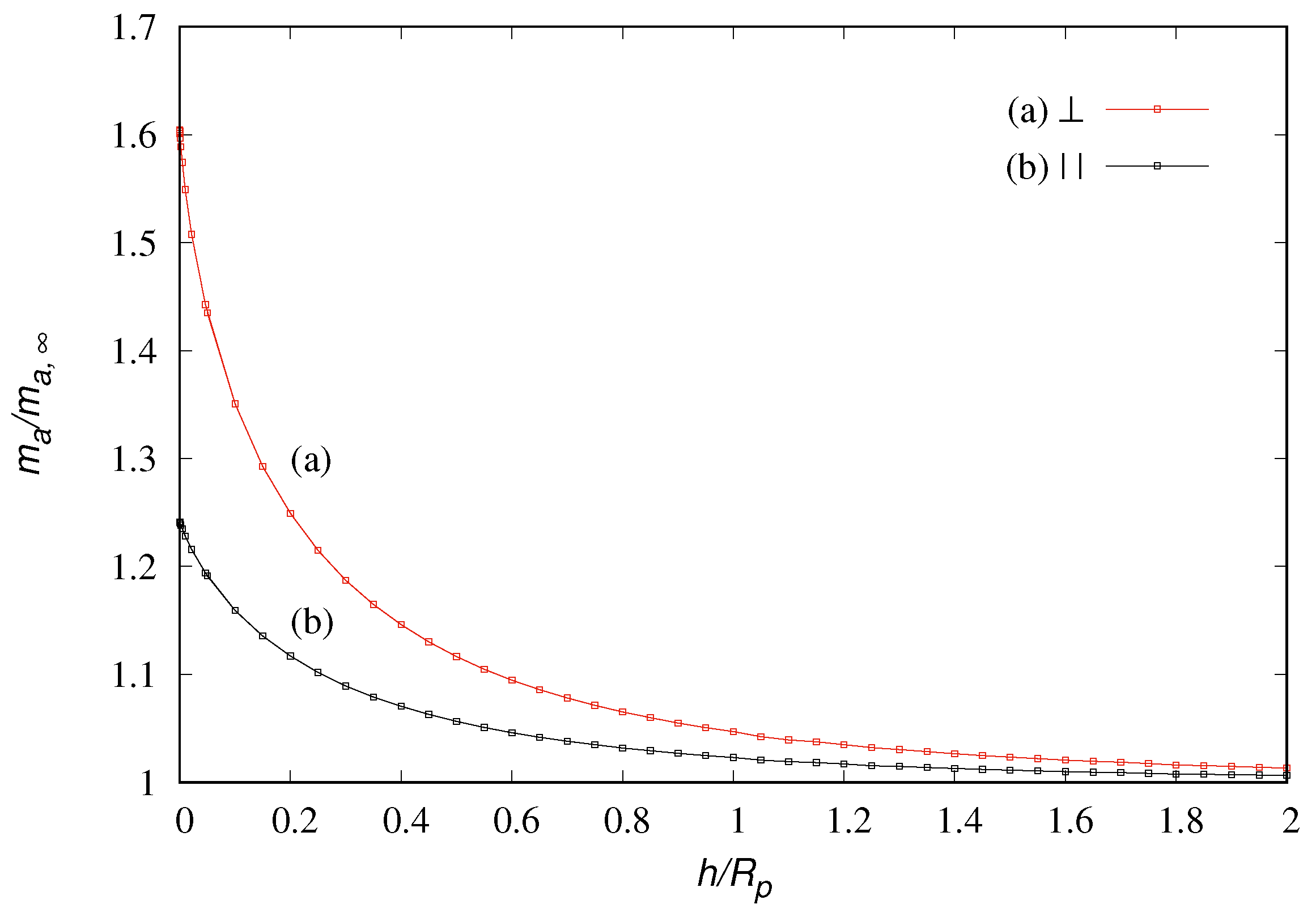
where is the particle volume, equal to half the mass of the fluid occupying the particle volume. Physically, the added mass contribution corresponds to the back action on the particle of the correlated motion of nearby fluid elements originating from the particle movement within the fluid [73]. In confined geometries, the added mass becomes a tensorial quantity dependent on particle position. For instance, for a spherical particle near a solid planar wall,
where , and , corresponding to the parallel and transversal added masses, are smooth functions of the particle distance from the wall, as depicted in Figure 5 attaining a finite value for .
Similarly, the Basset contribution attains in confined geometries a tensorial, position-dependent character,
where and . There are very few works on the characterization of the Basset force in confined geometries [74], and the detailed study of fluid inertial effects in microchannels and in the presence of solid walls represents an almost virgin field of theoretical and experimental investigation.
Gathering these contributions, and considering also the action of a potential and of a flow force , deriving e.g., by a (pressure-drive) flow in the fluid, the equations of motion for a microparticle become,
where is the stochastic fluctuational contributions, to be determined by enforcing fluctuation-dissipation relations. But also this aspect, owing to the explicit dependence of on the position , represents a challenging problem in statistical physics, especially if one is interested in determining the velocity autocorrelation function. Fortunately, for , corresponding to typical conditions in microfluidic applications, the fluid inertia can be neglected, and the stochastic description of particle motion can be based on the theory addressed in Section 2 and Section 3.
7. Concluding Remarks
Microfluidics is not only an emerging field as regards practical applications but it provides a fertile playground for analyzing fundamental physical questions. This is because particle motion at microscale is controlled by thermal stochastic fluctuations, the understanding of which would not only improve the performances of micofluidic devices (e.g. for separation purposes), but also could test the validity of classical physical theories (hydrodynamics) down to the scale where quantum effects should start to appear (going down to the nanoscale).
The fundamental peculiarity of microhydrodynamics in confined geometries is that fluid-particle interactions depend on the position and, owing to fluctuation-dissipation relations, these spatial nonuniformities are transferred to mass-transport properties (diffusion) giving rise to delicate theoretical issues and paradoxes.
As long as fluid inertia is negligible, it is still possible to derive a rather complete characterization of thermal fluctuations, and to perform a simplification of the equations of motion, eliminating the fast velocity variables, thus reducing the statistical description to the Fokker-Planck equation for the particle spatial density corresponding to a classical advection-diffusion equation in physical space and time. However, even in this case, transport paradoxes arise due to the singularity of the hydrodynamic resistances in the neighbourhood of a solid wall.
We have thoroughly analyzed how the lack of integrability of mass-transport models (diffusion equation) in the presence of a surface chemical reaction depend on the simplifying assumption of no-slip boundary conditions. The inclusion of slippage effects at all the solid surfaces (walls and particle) transforms the non-integrable -singularity in the transversal resistance coefficient near a planar wall into a logarithmic singularity (∼) resolving the above mentoned integrability problem. Hovewer, there are physical reasons to conjecture that a more refined modeling of fluid-particle interactions (including compressibility and acoustic effects) could completely eliminate the singularity in at the wall. This issue will be addressed in forthcoming works.
The inclusion of fluid inertia in confined microfluidics opens up other interesting and fundamental problems. The theoretical and numerical estimate of the Basset force even in simple confined systems is a basic ingredient in order to tackle the formulation of fluctuation-dissipation relations, and the efficient determination of the fluctuational force , similarly to what developed in the free space, in order to determine the short-time behavior of the velocity autocorrelation functions. In this framework, the development of more elaborate statistical physical methods should proceed hand-in-hand with the accurate experimental analysis of particle motion at short time and length scales near a solid surface, following and extending the experimental investigations recently performed for Brownian particles in the free space [75,76].
Author Contributions
Both authors contributed on equal footing to this work. All authors have read and agreed to the published version of the manuscript.
Funding
This research received no external funding.
Conflicts of Interest
The authors declare no conflict of interest.
Appendix A. Symmetry of the Resistance Matrix Independently of the Slippage
In order to show the symmetries of the matrices and, a-fortiori, of the overall matrix , in the presence of slip boundary conditions the Lorentz’s reciprocity theorem can be used as in [33]. Lorentz’s reciprocal theorem [60] states that given two solutions () and () of the Stokes’ Equation (5), the following identity holds
where is the fluid domain, its boundary and the normal unit vector to the boundary. Let us apply Equation (A1) to the problem of a particle moving in a bounded fluid domain considering two distinct solutions defined by the following slip boundary conditions
and
, being the strain rates
where and indicate the normal unit vectors to the surface of the particle and of the walls, respectively. The condition for applies solely if the fluid domain is unbounded, as in the case of Figure 1 The integral relation (A1) thus becomes
The boundary conditions Equation (A2) and (A3) can be substituted in the integrands entering Equation (A4). For example, the first integrand at the l.h.s. of Equation (A4) becomes
where the pressure term vanishes, since
Therefore,
In a similar way, the integrand on the surface of the particle at the r.h.s of Equation (A4) can be expressed as
The second term at the r.h.s of Equation (A8) is symmetric with respect to the indices , i.e.,
Therefore, these terms vanish in the Equation (A4) and so do the integrals on the surface of the walls. Since and are constant at the boundary, we have
where , , are the hydrodynamic forces acting upon the particle in the two problems considered. In the present case, the hydrodynamic resistance matrices depend on the slip lengths
so that the substitution of Equation (A11) into Equation (A10) yields
and consequently,
It is easy to recognize that the slip-dependent contributions mutually cancel out at the left and right hand sides of the Lorentz’s reciprocal relation also in the case of a rotating particle, where,
and
from which we obtain
A similar result occurs in application of Lorentz’s reciprocal relation to mixed problems, considering a translation boundary condition for , and a rotational one for , providing
Appendix B. Details on the FEM Simulations
The software COMSOL Multiphysics 5.4 has been used to perform FEM simulations. To take computational advantage from the axial symmetry of the problem of a sphere translating perpendicularly to a planar wall, for obtaining the coefficient in Equation (33), cylindrical coordinates have been used in a two dimensional square domain representing the fluid domain, with an empty disk, representing the spherical particle, possessing unit radius placed at distance h from planar wall.
The length of the sides of the square has been chosen much larger than the characteristic length of the physical problem (), so that their presence does not affect the resistance on the sphere, and a no-slip boundary condition has been imposed on these sides. Conversely, on the perimeter of the disk and on the nearest side (representing the planar wall), Navier’s slip conditions Equation (103) have been imposed to solve the Stokes’ problem Equation (5).
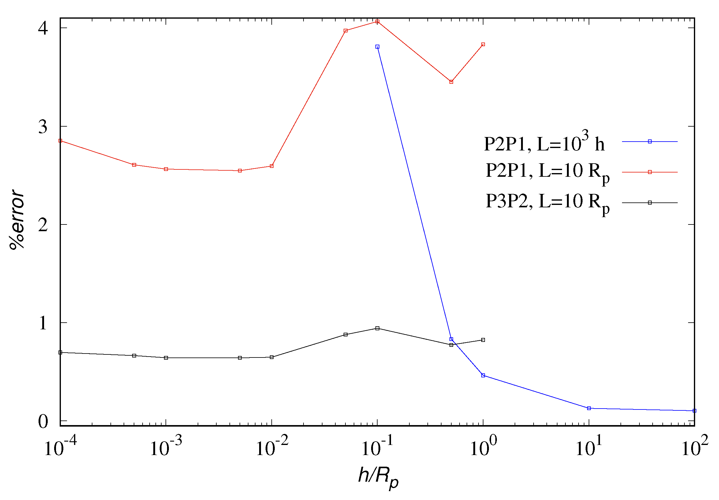
A finer mesh has been set on the perimeter of the disk representing the sphere, and the maximal length of the elements has been imposed to be less than . A quadratic shape order has been set to model the curvature of the circle and a double boundary layer with thickness about has been built around the circle, representing the surface of the sphere. The mesh in the square (fluid domain) has been modeled by imposing two different zones: a nearest zone of linear size with a maximum growth rate of the finite elements equal to , and an exterior zone with a higher growth rate of about 2. Both P2P1 and P3P2 finite elements have been used depending on the position of the particle. Figure A1 reports the data of the error analysis. The reference data for checking the numerical simulations are those of a no-slip particle moving parallel to a slip plane wall reported by Kezirian [77], obtained by the author solving the Stokes’ equations in bi-spherical coordinates. These data, to the best of our knowledge, are the only exact results regarding this kind of problem available in the literature. The percentage error has been evaluated by the relation
where refers to numerical simulations and to the data by [77].
Figure A1.
Percentual error (A19) of the FEM results for with respect to the data obtained by Kezirian [77] for a no-slip sphere translating parallel to a planar wall with slip length .

Figure A1 reports this comparison in three different cases. The data obtained by P2P1 element are accurate () for gaps larger than the radius of the particle. For smaller gaps, the dimension of the box can be considerably reduced since the total force depend principally on the hydrodynamic field in the gap. In this near field zone, pressure field is the leading term in the evaluation of the stress tensor [71]. Correspondingly, an improvement of the evaluation of the pressure field, obtained by non linear elements P3P2, yields accurate results with a percentage error less then .
The same parameters have been used for building both the geometry and the mesh for evaluating the added mass of a sphere moving near a plane wall. In this case, the fluid model used is a potential flow,
Therefore, for a given position of the sphere, three Laplace equations (one for each Cartesian axis )
has been solved by using Lagrangian quadratic elements, with the impermeability boundary conditions
where is the normal unit vector to the sphere and the velocity of the particle in the i-th direction. The entries of the added-mass matrix have been evaluated as [78],
References
- Einstein, A. Investigations on the Theory of Brownian Movement; Dover Publ.: Mineola, NY, USA, 1956. [Google Scholar]
- Cheng, T.-P. Einstein’s Physics; Oxford University Press: Oxford, UK, 2015. [Google Scholar]
- Langevin, P. Sur la theorie du mouvement brownien. Comptes Rendus de l’Académie des Sci. 1908, 146, 530–533. [Google Scholar]
- Cichocki, B. (Ed.) Marian Smoluchowski—Selected Scientific Works; WUW: Warsaw, Poland, 2017. [Google Scholar]
- Chandrasekhar, S. Stochastic problems in physics and astrophysics. Rev. Mod. Phys. 1943, 15, 1–89. [Google Scholar] [CrossRef]
- Venerus, D.C.; Öttinger, H.C. A Modern Course in Transport Phenomena; Cambridge University Pree: Cambridge, UK, 2018. [Google Scholar]
- Gorodetskyi, O.; Vivat, I.; Speetjens, M.F.; Anderson, P.D. Analysis of Advective–Diffusive Transport in Complex Mixing Devices by the Diffusive Mapping Method. Macromol. Theory Simul. 2015, 24, 322–334. [Google Scholar] [CrossRef]
- Cerbelli, S.; Garofalo, F.; Giona, M. Effective dispersion and separation resolution in continuous particle fractionation. Microfluid. Nanofluid. 2015, 19, 1035–1046. [Google Scholar] [CrossRef]
- Luni, C.; Michielin, F.; Barzon, L.; Calabró, V.; Elvassore, N. Stochastic Model-Assisted Development of Efficient Low-Dose Viral Transduction in Microfluidics. Biophys. J. 2013, 104, 934–942. [Google Scholar] [CrossRef] [PubMed] [Green Version]
- Bressloff, P.C.; Newby, J.M. Stochastic models of intracellular transport. Rev. Mod. Phys. 2013, 85, 135–196. [Google Scholar] [CrossRef] [Green Version]
- Klages, R.; Just, W.; Jarzynski, C. (Eds.) Nonequlibrium Statistical Physics of Small Systems; Wiley-VCH: Weinheim, Germany, 2013. [Google Scholar]
- Coffey, W.; Kalmykov, Y.P. The Langevin Equation: With Applications to Stochastic Problems in Physics, Chemistry and Electrical Engineering; World Scientific: Singapore, 2012. [Google Scholar]
- Zinn-Justin, J. From Random Walks to Random Matrices—Selected Topics in Modern Theoretical Physics; Oxford University Press: Oxford, UK, 2019. [Google Scholar]
- Kubo, R. The fluctuation-dissipation theorem. Rep. Prog. Phys. 1966, 29, 255–284. [Google Scholar] [CrossRef] [Green Version]
- Kubo, R.; Toda, M.; Hashitsume, N. Statistical Physics II—Nonequilibrium Statistical Mechanics; Springer: Berlin, Germany, 1991. [Google Scholar]
- Karniadakis, G.; Beskok, A. Aluru, N. Microflows and Nanoflows—Fundamentals and Simulation; Springer: New York, NY, USA, 2005. [Google Scholar]
- Ehrfeld, W.; Hessel, V.; Löwe, H. Microreactors; Wiley-VCH: Weinheim, Germany, 2000. [Google Scholar]
- Whitesides, G.M. The origin and the future of microfluidics. Nature 2006, 442, 368–373. [Google Scholar] [CrossRef]
- Hardt, S.; Schönfeld, F. (Eds.) Microfluidic Thechnologies for Miniaturized Analysis Systems; Springer: New York, NY, USA, 2007. [Google Scholar]
- Bruus, H. Theoretical Microfluidics; Oxford University Press: Oxford, UK, 2008. [Google Scholar]
- Mo, J.; Raizen, M.G. Highly resolved Brownian motion in space and in time. Annu. Rev. Fluid Mech. 2019, 51, 403–428. [Google Scholar] [CrossRef]
- Pesce, G.; Jones, P.H.; Maragò, O.M.; Volpe, G. Optical tweezers: Theory and practice. Eur. Phys. J. Plus 2020, 135, 949. [Google Scholar] [CrossRef]
- Bousse, L.; Cohen, C.; Nikiforov, T.; Chow, A.; Kopf-Sill, A.R.; Dubrow, R.; Parce, J.W. Electrokinetically controlled microfluidic analysis systems. Annu. Rev. Biophys. Biomol. Struct. 2000, 29, 155–181. [Google Scholar] [CrossRef] [PubMed]
- Chang, C.C.; Yang, R.J. Electrokinetic mixing in microfluidic systems. Microfluid. Nanofluid. 2007, 3, 501–525. [Google Scholar] [CrossRef]
- Kirby, B.J. Micro- and Nanoscale Fluid Mechanics; Cambridge University Press: Cambridge, UK, 2010. [Google Scholar]
- Petersson, F.; Aberg, L.; Swärd-Nilsson, A.M.; Laurell, T. Free flow acoustophoresis: Microfluidic-based mode of particle and cell separation. Anal. Chem. 2007, 79, 5117–5123. [Google Scholar] [CrossRef] [PubMed]
- Urbansky, A.; Ohlsson, P.; Lenshof, A.; Garofalo, F.; Scheding, S.; Laurell, T. Rapid and effective enrichment of mononuclear cells from blood using acoustophoresis. Sci. Rep. 2017, 7, 17161. [Google Scholar] [CrossRef]
- Volpe, G.; Helden, L.; Brettschneider, T.; Wehr, J.; Bechinger, C. Influence of Noise on Force Measurements. Phys. Rev. Lett. 2010, 104, 170602. [Google Scholar] [CrossRef] [Green Version]
- Brettschneider, T.; Volpe, G.; Helden, L.; Wehr, J.; Bechinger, C. Force measurement in the presence of Brownian noise: Equilibrium-distribution method versus drift method. Phys. Rev. E 2011, 83, 041113. [Google Scholar] [CrossRef] [Green Version]
- Mo, J.; Simha, A.; Raizen, M.G. Brownian motion as a new probe of wettability. J. Chem. Phys. 2017, 146, 134707. [Google Scholar] [CrossRef] [Green Version]
- Mohideen, U.; Roy, A. Precision Measurement of the Casimir Force from 0.1 to 0.9 μm. Phys. Rev. Lett. 1998, 81, 4549–4552. [Google Scholar] [CrossRef] [Green Version]
- Bordag, M.; Klimchitskaya, G.L.; Mohideen, U.; Mostepanenko, V.M. Advances in the Casimir Effect; Oxford University Press: Oxford, UK, 2015. [Google Scholar]
- Happel, J.; Brenner, H. Low Reynolds Number Hydrodynamics: With Special Applications to Particulate Media; Martinus Nijhoff: The Hague, The Netherlands, 1983. [Google Scholar]
- Kim, S.; Karrila, S.J. Microhydrodynamics—Principles and Selected Applications; Dover Publ.: Mineola, NY, USA, 2005. [Google Scholar]
- Stokes, G.G. On the Theories of the Internal Friction of Fluids in Motion and of the Equilibrium and Motion of Elastic Solids. Trans. Camb. Philos. Soc. 1945, 8, 287–319. [Google Scholar]
- Brady, J.F.; Bossis, G. Stokesian dynamics. Annu. Rev. Fluid Mech. 1988, 20, 111–157. [Google Scholar] [CrossRef]
- Segre, G.; Silberberg, A.J. Behaviour of macroscopic rigid spheres in Poiseuille flow Part 1. Determination of local concentration by statistical analysis of particle passages through crossed light beams. J. Fluid Mech. 1962, 14, 115–135. [Google Scholar] [CrossRef]
- Segre, G.; Silberberg, A. Behaviour of macroscopic rigid spheres in Poiseuille flow Part 2. Experimental results and interpretation. J. Fluid Mech. 1962, 14, 136–157. [Google Scholar] [CrossRef]
- Ho, B.P.; Leal, L.G. Inertial migration of rigid spheres in two-dimensional unidirectional flows. J. Fluid Mech. 1974, 65, 365–400. [Google Scholar] [CrossRef]
- Galletti, C.; Roudgar, M.; Brunazzi, E.; Mauri, R. Effect of inlet conditions on the engulfment pattern in a T-shaped micro-mixer. Chem. Eng. J. 2012, 185, 300–313. [Google Scholar] [CrossRef]
- Mariotti, A.; Galletti, C.; Mauri, R.; Salvetti, M.V.; Brunazzi, E. Steady and unsteady regimes in a T-shaped micro-mixer: Synergic experimental and numerical investigation. Chem. Eng. J. 2018, 341, 414–431. [Google Scholar] [CrossRef]
- Borgogna, A.; Murmura, M.A.; Annesini, M.C.; Giona, M.; Cerbelli, S. Inertia-driven enhancement of mixing efficiency in microfluidic cross-junctions: A combined Eulerian/Lagrangian approach. Microfluid. Nanofluid. 2018, 22, 1–15. [Google Scholar] [CrossRef]
- Burada, P.S.; Hänggi, P.; Marchesoni, F.; Schmid, G.; Talkner, P. Diffusion in confined geometries. Chem. Phys. Chem 2009, 10, 45–54. [Google Scholar] [CrossRef]
- Bezrukov, S.M.; Schimansky-Geier, L.; Schmid, G. Brownian motion in confined geometries. Eur. Phys. J. Spec. Top. 2014, 223, 3021–3025. [Google Scholar] [CrossRef]
- Gardiner, C. Stochastic Methods; Springer: Berlin, Germany, 2009. [Google Scholar]
- Golub, G.H.; Van Loan, C.F. Matrix Computations; North Oxford Academic: Oxford, UK, 1983. [Google Scholar]
- Van Kampen, N.G. It versus Stratonovich. J. Stat. Phys. 1981, 24, 175–187. [Google Scholar] [CrossRef]
- Mannella, R.; McClintock, P.V.E. Ito versus Stratonovich: 30 years later. Fluct. Noise Lett. 2012, 11, 1240010. [Google Scholar] [CrossRef] [Green Version]
- Sancho, J.M.; San Miguel, M.; Dürr, D. Adiabatic elimination for systems of Brownian particles with nonconstant damping coefficients. J. Stat. Phys. 1982, 28, 291–305. [Google Scholar] [CrossRef]
- Wong, E.; Zakai, M. On the Convergence of Ordinary Integrals to Stochastic Integrals. Ann. Math. Stat. 1965, 36, 1560–1564. [Google Scholar] [CrossRef]
- Wong, E.; Zakai, M. Riemann-Stieltjes Approximations of Stochastic Integrals. Zeitschrift für Wahrscheinlichkeitstheorie und Verwandte Gebiete 1969, 12, 87–97. [Google Scholar] [CrossRef]
- Kloeden, P.E.; Platen, E. Numerical Solutution of Stochastic Differential Equations; Springer: Berlin, Germany, 2010. [Google Scholar]
- Lancon, P.; Batrouni, G.; Lobry, L.; Ostrowsky, N. Drift without flux: Brownian walker with a space-dependent diffusion coefficient. Europhys. Lett. 2001, 54, 28–33. [Google Scholar] [CrossRef] [Green Version]
- Lancon, P.; Batrouni, G.; Lobry, L.; Ostrowsky, N. Brownian walker in a confined geometry leading to a space-dependent diffusion coefficient. Physica A 2002, 304, 65–76. [Google Scholar] [CrossRef]
- Duhr, S.; Braun, D. Thermophoretic depletion follows Boltzmann distribution. Phys. Rev. Lett. 2006, 96, 168301. [Google Scholar] [CrossRef] [PubMed] [Green Version]
- Hottovy, S.; Volpe, G.; Wehr, J. Thermophoresis of Brownian particles driven by coloured noise. Europhys. Lett. 2012, 99, 60002. [Google Scholar] [CrossRef] [Green Version]
- De Groot, S.R.; Mazur, P. Non-Equilibrium Thermodynamics; Dover Publ.: Mineola, NY, USA, 1984. [Google Scholar]
- Cox, R.G. The motion of suspended particles almost in contact. Int. J. Multiph. Flow 1974, 1, 343–371. [Google Scholar] [CrossRef]
- Cox, R.G.; Brenner, H. The slow motion of a sphere through a viscous fluid towards a plane surface—II Small gap widths, including inertial effects. Chem. Eng. Sci. 1967, 22, 1753–1777. [Google Scholar] [CrossRef]
- Lorentz, H.A. Abhandlungen über Theoretische Physik; BG Teubner: Leipzig/Berlin, Germany, 1907. [Google Scholar]
- Dussan, V.E.B.; Davis, S. On the motion of a fluid-fluid interface along a solid surface. J. Fluid Mech. 1974, 65, 71–95. [Google Scholar] [CrossRef]
- Moffatt, H.K. Viscous and resistive eddies near a sharp corner. J. Fluid Mech. 1964, 18, 1–18. [Google Scholar] [CrossRef] [Green Version]
- Dussan, V.E.B. The moving contact line: The slip boundary condition. J. Fluid Mech. 1976, 77, 665–684. [Google Scholar] [CrossRef]
- Wang, C.Y. Lid-driven Stokes slip flow in a rectangular cavity. Eur. J. Mech. B Fluids 2021, 89, 93–99. [Google Scholar] [CrossRef]
- Goldstein, S. Modern Developments in Fluid Dynamics: An Account of Theory and Experiment Relating to Boundary Layers, Turbulent Motion and Wakes; Dover Publ.: Mineola, NY, USA, 1965. [Google Scholar]
- Navier, C.L.M.H. Mémoire sur les lois du mouvement des fluides. Mémoires de l’Académie Royale des Sciences de l’Institut de France 1823, 6, 389–440. [Google Scholar]
- Lauga, E.; Brenner, M.; Stone, H. Microfluidics: The No-Slip Boundary Condition. In Springer Handbook of Experimental Fluid Mechanics; Tropea, C., Yarin, A.L., Foss, J.F., Eds.; Springer: Berlin, Germany, 2007; pp. 1219–1240. [Google Scholar]
- Eslami, H.; Muller-Plathe, F. Viscosity of nanoconfined polyamide-6, 6 oligomers: Atomistic reverse nonequilibrium molecular dynamics simulation. J. Phys. Chem. B 2010, 114, 387–395. [Google Scholar] [CrossRef]
- Landau, L.D.; Lishitz, E.M. Statistical Physics, Part 1, 3rd ed.; Elsevier: Amsterdam, The Netherlands, 2013. [Google Scholar]
- Basset, A.B. A Treatise on Hydrodynamics: With Numerous Examples; Deighton, Bell and Company: Cambridge, UK, 1888; Volume 2. [Google Scholar]
- Hocking, L.M. The effect of slip on the motion of a sphere close to a wall and of two adjacent spheres. J. Eng. Math. 1973, 7, 207–221. [Google Scholar] [CrossRef]
- Goren, S.L. The hydrodynamic force resisting the approach of a sphere to a plane permeable wall. J. Colloid Interface Sci. 1979, 69, 78–85. [Google Scholar] [CrossRef]
- Darwin, C. Note on hydrodynamics. Math. Proc. Camb. Philos. Soc. 1953, 49, 342–354. [Google Scholar] [CrossRef]
- Simha, A.; Mo, J.; Morrison, P.J. Unsteady Stokes flow near boundaries: The point-particle approximation and the method of reflections. J. Fluid Mech. 2018, 841, 883–924. [Google Scholar] [CrossRef] [Green Version]
- Huang, R.; Chavez, I.; Taute, K.M.; Lukic, B.; Jeney, S.; Raizen, M.G.; Florin, E.L. Direct observation of the full transition from ballistic to diffusive Brownian motion in a liquid. Nat. Phys. 2011, 7, 576–580. [Google Scholar] [CrossRef]
- Kheifets, S.; Simha, A.; Melin, K.; Li, T.; Raizen, M.G. Observation of Brownian motion in liquids at short times: Instantaneous velocity and memory loss. Science 2014, 343, 1493–1496. [Google Scholar] [CrossRef] [PubMed]
- Kezirian, M.T. Hydrodynamics with a Wall-Slip Boundary Condition for a Particle Moving near a Plane Wall Bounding a Semi-Infinite Viscous Fluid. Ph.D. Thesis, Massachusetts Institute of Technology, Cambridge, MA, USA, 1992. [Google Scholar]
- Ghassemi, H.; Yari, E.M. The Added Mass Coefficient computation of sphere, ellipsoid and marine propellers using Boundary Element Method. Pol. Marit. Res. 2011, 18, 17–26. [Google Scholar] [CrossRef] [Green Version]
Figure 1.
Schematic representation of a spherical particle near an infinitely extended planar wall.

Figure 2.
Dimensionless hydrodynamics resistance coefficient vs for equal slip lengths on the particle surface and on the wall. Each color in the figure corresponds to a different slip length as described in the inner legend. Continuous lines represent the results of the Goren’s equations, dotted lines the values obtained by the Hocking’s equation Equation (104), and symbols the results of FEM simulations.

Figure 3.
Dimensionless hydrodynamics resistance coefficient vs in the case no-slip boundary conditions are imposed at the surface of the sphere (a) or at the wall (b). Each color in the panels corresponds to a different combination of slip lengths as described in the inner legends. Continuous lines represent the results of the Goren’s equations, symbols the results of FEM simulations.

Figure 4.
Dimensionless hydrodynamics resistance coefficient vs obtained by keeping fixed the slip length on the i-th surface () and varying the slip length on the other obtained by solving the Goren’s equations. Observe that the curves corresponding to and practically overlap in this range of parameter values.

Figure 5.
Ratio of the added mass of a sphere moving perpendicular (, red line) and parallel (, black line) to a planar wall to that in an unbounded fluid obtained by FEM simulations.
Figure 5.
Ratio of the added mass of a sphere moving perpendicular (, red line) and parallel (, black line) to a planar wall to that in an unbounded fluid obtained by FEM simulations.

Publisher’s Note: MDPI stays neutral with regard to jurisdictional claims in published maps and institutional affiliations. |
© 2022 by the authors. Licensee MDPI, Basel, Switzerland. This article is an open access article distributed under the terms and conditions of the Creative Commons Attribution (CC BY) license (https://creativecommons.org/licenses/by/4.0/).
Share and Cite
MDPI and ACS Style
Procopio, G.; Giona, M. Stochastic Modeling of Particle Transport in Confined Geometries: Problems and Peculiarities. Fluids 2022, 7, 105. https://doi.org/10.3390/fluids7030105
AMA Style
Procopio G, Giona M. Stochastic Modeling of Particle Transport in Confined Geometries: Problems and Peculiarities. Fluids. 2022; 7(3):105. https://doi.org/10.3390/fluids7030105
Chicago/Turabian StyleProcopio, Giuseppe, and Massimiliano Giona. 2022. "Stochastic Modeling of Particle Transport in Confined Geometries: Problems and Peculiarities" Fluids 7, no. 3: 105. https://doi.org/10.3390/fluids7030105