
A Power Sequence Interaction Function for Liquid Phase Particles

FABES Forschungs-GmbH, Schragenhofstr. 35, D-80992 München, Germany
Fluids 2021, 6(10), 354; https://doi.org/10.3390/fluids6100354
Submission received: 17 August 2021
/
Revised: 20 September 2021
/
Accepted: 20 September 2021
/
Published: 8 October 2021
(This article belongs to the Special Issue Thermodynamic Properties of Liquid Mixtures)
Abstract
:In this manuscript, a function is derived that allows the interactions between the atoms/molecules in nanoparticles, nanodrops, and macroscopic liquid phases to be modeled. One goal of molecular theories is the development of expressions to predict specific physical properties of liquids for which no experimental data are available. A big limitation of reliable applications of known expressions is that they are based on the interactions between pairs of molecules. There is no reason to suppose that the energy of interaction of three or more molecules is the sum of the pairwise interaction energies alone. Here, an interaction function with the limit value w = e2π/e is presented, which allows for the derivation of the atomic mass unit and acts as a bridge between properties of elementary particles and emergent properties of macroscopic systems. The following properties of liquids are presented using the introduced interaction function: melting temperatures of n-alkanes, nanocrystals of polyethylene, melting temperatures of metal nanoparticles, solid–liquid phase transition temperatures for water in nanopores, critical temperatures and critical pressures of n-alkanes, vapor pressures in liquids and liquid droplets, self-diffusion coefficients of compounds in liquids, binary liquid diffusion coefficients, diffusion coefficients in liquids at infinite dilution, diffusion in polymers, and viscosities in liquids.
1. Introduction
Macroscopic systems of atoms and molecules exist as gases, liquids, and solids. The starting point for the discussion of gases is the completely disordered distribution of the molecules of a perfect gas without a specific volume. The starting point for the discussion of solids is the ordered structure of a perfect crystal. Liquids lie between these two extremes. The potential energy of the particles in the liquid, responsible for the attractive interaction, is of the same order of magnitude as the kinetic energy. The consequence is a mobile structure, but with a specific volume, which considerably complicates the theoretical treatment of liquids. However, it is just these properties that determine the exceptional importance of liquids to the high variety of material systems, including living matter.
Macroscopic systems have emergent properties unknown for individual particles, like temperature, as an example. Expressions for bulk properties can be obtained from statistical mechanics. With these expressions, properties of macroscopic systems can be interrelated through a common link of intermolecular force laws. The Molecular Theory of Gases and Liquids, published by Hirschfelder et al. in 1954 [1], describes the interactions between two molecules in terms of functions based on quantum mechanics.
However, emergent properties are very difficult to reduce to just interactions between pairs of particles without consideration of the other nearby particles. An attempt to consider more than one pair resulted in the Axilrod–Teller equation [2], but without significant improvement.
An enormous number of methods has been published for modeling liquid properties, as shown in the book The Properties of Gases and Liquids by Poling et al. [3]. All models use partially empirical structures with several empirical constants. Predictions with reliable results, based only on interactions between pairs of particles, need sophisticated algorithms and high computational efforts.
This complex modeling situation is the reason for this investigation, in which a reliable assumption of the interaction basis, combined with a maximum of simplicity for practical applications, is the main goal for prediction modeling of liquid properties.
2. The Interaction Function
A first physical assumption for an interaction model is a system of uniform particles with equal finite energies. This is also a basic assumption of quantum mechanics. The N particles of the system form n groups of x1, x2, …, xn particles. For modeling possible interactions between these particles, the physical system is correlated with the system of natural numbers. The n groups are correlated with the n natural numbers x1, x2, …, xn. With this correlation a connection with the fundamental laws of arithmetic is established.
A fundamental law of natural numbers is the relation g ≤ m between the arithmetical mean m = (x1 + x2 + … + xn)/n = N/n and the geometrical mean g = (x1·x2·…·xn)1/n. The general theorem states that the extreme value g = m is valid only if all the xi numbers are equal. This property is used as starting point for comparisons with physical systems consisting of uniform particles. A consequence of the maximum g = m is a system of uniform groups of unities. Such uniformity of elementary particles, atoms, and molecules of a specific structure is a characteristic property of matter.
However, in addition to the extreme g = m, the following relations with further extreme values result. If the natural number N can be written in different ways as a sum of ni identical prime numbers xi as a result of g = m, then the corresponding product yi = xini has a maximum value of xi = 3, as shown in the following examples where ni xi = N = 30.

| xi | ni | yi = xini = xiN/xi |
|---|---|---|
| 2 | 15 | 32,768 |
| 3 | 10 | 59,049 |
| 5 | 6 | 15,625 |
This property of grouping natural numbers leads to the function
y = xq/x with q ≥ 1 and the maximum value ymax = 3q/3 for x = 3.
With xi >> 1 and (1 + 1/xi)xi = e = 2.71828…, the value Ymax = eq/e > ymax = 3q/3 is the result (Figure 1).
The functions ymax and Ymax in Equation (1) represent a form of collective organization in the system of natural numbers. The fundamental additive (extensive) and multiplicative (intensive) rules in arithmetic lead to microsystems made of three particles with a maximum relative intensity of interaction represented as ymax, and to macrosystems made of x >> 1 particles, with a maximum relative intensity of interaction represented as Ymax in Equation (1).
Although not decisive for the following, the xi interacting particles in Equation (1) can be treated mathematically as a permutation. The process can be understood formally as x! interacting steps. Each individual step is interpreted mathematically as one change of places between two numbers. The total number of such place exchanges is x!. The relative number px of exchanges related to x! with no particle remaining in its starting position is then [4]:
px = 1/2! − 1/3! + ….+ (−1)x 1/x!, where lim px = pe = 1/e for x >> 1.
The limit value pe = 1/e is designated as the maximum probability of a place exchange in the system. In this model it is assumed that the interaction between uniform particles in the system occurs with the maximum probability eq·pe = eq/e.
Now a second fundamental assumption for the physical system is introduced with the number 2π. The first assumption of a finite energy says nothing about the dimension of the initial particles. Assuming a spherical particle with the relative radius r = 1, a circumference of 2π is the result. In conformity with quantum mechanics, any particle traveling with a linear momentum p should have a wavelength λ given in the de Broglie relation p = h/λ, with Planck’s constant h. With a relative wavelength λ = 2π, a new initial value q = 2π is introduced into Equation (1) instead of q = 1, and the following number, w = e2π/e, is the result for the maximum value Ymax in macrosystems. In this way a combination of arithmetic and geometry occurs.
The number w represents the limit value of the following power sequence [5,6]:
with the limit value:
where w1 = (1 + 2π)1/2 = 2.6987…and w1,e = (1 + 2π)1/e = 2.076…
The power sequence in Equation (3) is denoted in the following as the interaction function. The limit value w represents a relative energy density in the macrosystem.
A first application of the interaction function starts with the term w1 in Equation (3). This is the first term, where n = 1 in the power sequence and with the same limit value w as in Equation (3).
In conformity with the Einstein equation E = mc2, a body at rest has a rest energy (mass energy) of E0 = m0·c2, with the speed of light c.
The value w1 represents the relative energy of one elementary particle. In conformity with Equation (1), a maximum of interaction is the result with a combination of three elementary particles, and this leads to ymax = 3q/3 = w13 = 19.6554, with a value q = 8.1330397 and q/3 = 2.711…≈ e. Now, with E13 = 1/[exp(w13)·w13] = 1.48 × 10⁻¹⁰, the relative rest energy is defined as resulting from the three interacting particles w1.
In order to transform the relative energy value w1 into a quantity expressed in IS units, the limit value w in Equation (3) must be related to the decimal system with the basic number 10. In this way w1·w/10 represents the energy as J.
That means the rest energy E0 = E13·w/10 J = 1.49326 × 10⁻¹⁰ J, and with c = 2.99792458 × 10⁸ ms−1 the theoretical atomic mass unit u0 = m0 = E0/c2 = 1.661475 × 10⁻²⁷ kg ≈ 1.66054 × 10⁻²⁷ kg = u [7] is the result.
The interaction function is of fundamental importance for emergent properties in fluid phases and the first term w1 forms a bridge between the fundamental atomic mass unit and macroscopic properties. This connection explains the importance of the relative mass values M of particles in macroscopic systems related to the n-alkanes with i carbon atoms, as reference homologous series for all organic substances, and the term (M − 2)/14 = i = n in from Equation (3).
3. The Interaction Function and the Optimal Entropy
The next application of the interaction function refers to emergent properties of fluids. The starting point is a system with one mol of uniform particles with a relative molar energy w1 = (1 + 2π)0.5. If these particles interact in conformity with Equation (3), the limit of relative molar energy w = e2π/e is the result for a fluid phase. This is a reference value resulting from optimal interaction of uniform particles in a liquid phase as a consequence of Equation (1) where q = 2π. However, if no interactions occur between the n particles, then w1,e = (1 + 2π)1/e represents the fluid phase in this situation as a limit value for n >> 1. This can be understood as the critical state of a system without interactions and holds for a liquid as well as for a gas phase, with a compression factor Z = 1. However, the term w1 = (1 + 2π)1/2 in Equation (3) represents the relative molar energy of a perfect gas phase. That means that a supplementary relative internal molar kinetic energy Eint related to the difference w1 − w1,e exists in the system. This energy determines a certain temperature T.
In order to establish a connection between the difference w1 − w1,e and SI units, start with n = 1000 mol of hypothetical particles with the atomic mass unit u = 1.66 × 10⁻²⁷ kg in a volume V = 1 m3 and the Avogadro constant NA. This system, where N = n·NA = 103 (mol) × 6.02214 × 10²³ (mol−1) particles, defines the mass unit of N·u = 1.000 kg. The total energy of the system is E = ∑ni, where ni particles with energy εi and the total number of particles is N = ∑ni. Using the Boltzmann distribution, E = (N/q) ∑exp(−), where = 1/kT and the translational partition function is q [7]. The following relationship between N/q and the two terms w1 and w1,e is now postulated:
This takes into account the relative internal molar kinetic energy w1 − w1,e.
With the translational partition function q = N/(w1 − w1,e) = V/λ3 and λ3 = h3/(2πu0kT)3/2, a value of T = 2.98058 K is the result, using the previous values for N, V, u, the Planck constant h = 6.62607015 × 10⁻³⁴ Js, the Boltzmann constant k = 1.380649 × 10⁻²³ JK−1, and the thermal de Broglie wavelength λ.
The self-diffusion of particles and the entropy of a system are both a result of random particle motion. With the Sackur–Tetrode equation, the molar entropy Sm of the above system can be calculated at temperature T and pressure P:
where λ3 = 1.03407 × 10⁻²⁷ for T = 2.98058 K and P = 1 Pa, and the value of Sm = 108.85 JK−1mol−1 results from Equation (5), with the gas constant R = 8.31447 JK−1mol−1.
The same value results for T = 298.058 K and P = 105 Pa. The internal energy of the gas phase at T = 2.98058 K is RT = 24.78 J mol−1.
The consequence of the above result is an optimum value of molar entropy for fluid systems at T = 298 K and P = 1 bar. At these conditions a maximum of the variety in the structure of matter (including living matter) occurs. As an example, the many enzyme reactions in water at room temperature can be mentioned. In the range of 273 < T < 373 K and 0.7 < P < 1.7 bar, deviations of the entropy from 108 JK−1mol−1 are < 7%.
It can be supposed that the natural evolution occurs not only in the direction of increasing entropy, but also in the direction of increasing the variety of structures. Of course, the necessary conditions for such macroscopic systems are assumed, which occur with low probability in the known world.
The liquid phase is determined in the temperature range between the freezing point Tf, the boiling point Tb, and the critical temperature Tc with the critical pressure Pc, which means Tf ≤ T ≤ Tc.
In conformity with classic statistical mechanics, the molar volume heat capacity of monoatomic solids is CV,m = 3R JK−1mol−1 (Dulong–Petit rule). This rule is valid only at high temperatures, as demonstrated with quantum mechanics (Einstein and Debye), where CV,m = 0 at T = 0. The molar entropy of melting, Sm,S, is for many monoatomic solids < 3R. One reason is the existence of several phase transitions in the solid state [8]. Here a molar entropy of Sm,S = 3R JK−1 mol−1 is assumed at Tf. For the molar entropy of liquid evaporation, a value of Sm,L = R·w = 83.9 K−1mol−1 has been defined [5] (Troutons law). That means a total molar entropy results for a gas phase, Sm,G = R(3 + w) = 108.83 JK−1mol−1, in the above optimal situation, in conformity with Equations (4) and (5) with the value 108.85 JK−1mol−1.
The molar entropy change for the isothermal expansion of a perfect gas is ΔS = R·ln(V2/V1) JK−1mol−1. When V2 = 2.479 × 10⁻² m3mol−1 for the molar volume of the perfect gas at 298.15 K, the value V1 = 1.03 × 10⁻⁶ m3mol−1 = 1.03 cm3mol−1 results for the molar volume of gas in a mol of liquid, independent of its composition [8].
4. Modeling of Liquid-Phase Properties with the Interaction Function
All prediction equations presented in the following are based on the interaction function of Equation (3). Its application fell into two categories [5]:
- Prediction of physical properties of nanoparticles or drops made of a limited number n of atoms or molecules as functions of n, with an asymptotical limit value for n >> 1. With specific constants C and corresponding dimensions with basic IS units, the energy En = Cwn of corresponding nanoparticles and E = Cw for macrosystems is the result.
- Prediction of physical properties of macroscopic systems with molecules from a homologous series, like n-alkanes, with i carbon atoms. When Ei = C0wi,ew the energy of a macrosystem can be defined that contains molecules from a homologous series with i identical atomic groups in each molecule, then the dimensionless ratio Ei/E∞ = C0wi,ew/C0ww = wi,e/w is the result.
That means, even one molecule can be treated as a system of i interacting subparticles in conformity with the interaction function defined in Equation (3). The non-polar Methylene group -CH2- with two strong covalent bonded H-atoms is such a subparticle, with a certain individuality along the i carbon atoms in the chain. This is in contrast to the situation in a strong polar molecule, like water, with three atoms with a relative free mobility to each other.
Such predictions can be generalized for any organic compound with the relative molecular mass M and different polarity and structure, with an additional specific parameter for that molecule.
The property of chain formation is characteristic for organic compounds and the n-alkanes are therefore the reference series for all organic compounds [5,6].
The structure of this series with i carbon atoms and relative molecular masses of Mi = 14·i + 2 delivers a basis for the correlation of emergent properties of fluid systems with the interaction function of Equation (3). The relative molecular mass M of a compound can be related to the number i = (M − 2)/14, corresponding to a hypothetical alkane with i carbon atoms. When i = n the interaction function wn,e is used.
Compounds of the first category above, for example monoatomic systems, are correlated with the first term w1,e of the interaction function.
The different emergent properties of liquid systems result as exponential functions. The specific polarity and specific structure of a compound is taken into account with an increment. This increment results often in the formation of a temperature-dependent factor f = a + bT or f = a + b/T. The relative simplicity of this temperature dependence results from the exponential form of most prediction equations, with the increment f in the exponent. This increment can be included in n = (M − 2 + f)/14 or can be used as a separate parameter in the prediction equation for the corresponding property. The uniform treatment of all these properties, based on wn,e, allows for a significant reduction in the use of additional empirical factors to a minimum, because the derived prediction equations have a real connection to the corresponding properties. The two empirical terms a and b in this increment term compensate for the approximations resulting from the simplifications used. The assignment of these increments to specific functional groups and structures is important. If experimental values for a property under consideration are available for the most important functional groups and specific structures, then a map of such values may be a helpful basis for estimations of values for unknown cases.
In the following, examples of emergent properties are discussed in connection with phase transitions, like melting or freezing points (Tm and Tf, respectively) and vapor pressures Pvp, until the critical temperature Tc at equilibrium, and with dynamic processes, such as diffusion coefficients DL and viscosity coefficients ηL in liquids and diffusion coefficients DP of compounds in polymers.
It is obvious that two values obtained for two temperatures for a single specific parameter, related to the relative molecular mass M, can offer only an approximation of the requested property. However, if such simple results obtained for various functional groups and specific structures are in the same order of magnitude as results from sophisticated models that are based on several empirical constants with the need for high computational effort, it is more advantageous to use the simpler way.
4.1. Modeling Melting Temperatures of n-Alkane Macrosystems Using the Interaction Function
The melting or freezing point of a pure substance is one of the most important specific macroscopic properties for its characterization and identification. It is also a specific parameter for crystalline polymers. The stability of alkane crystalline structures results from two types of interactions: lateral association of chains with interactions in the x- and y-directions and interactions in the z direction across gaps between methyl end groups [9]. The melting point of a macroscopic alkane crystal sample is the result of the different orientations of the molecules along the coordination axis, but is determined mainly by the chain length of the molecules, e.g., by the number i of the methylene groups (particles), including the two methyl end groups, because the molecular interfaces are proportional to i. One can assume that the main interactions occur along the x- and y-directions and are proportional to an interaction function wi,e. However, the interaction between the two methyl groups from two neighbor molecules along the z-direction must also be taken into account. Therefore, a constant with a smaller value than wi,e must be used for the z-axis. The ratio w1/wi,e, where w1 = (1 + 2π)1/2, was found to be the best approximation for the relative interaction in the z-direction. The ratio of the melting point of an alkane with i C-atoms Tm,i and the limit value Tm,∞ for i >> 1 can then be described by the following equation:
In order to determine the limit value Tm,∞, accurate melting points of known alkanes are necessary.
From the experimental melting temperatures Tm,i of the n-alkanes [10] the corresponding limit values were calculated with Equation (6). The first few members of the homologous series did not show a regular increase in their melting points with carbon number. This irregularity was caused by crystal structural differences between molecules with even and odd i-values as well as by the methyl end groups. To avoid these effects, alkane molecules from i > 23 were selected from [10].
In addition, the melt temperature of Tm,192 = 400.65 K was determined [11] at the equilibrium between the molten and crystalline state for the synthesized straight-chain alkane C192H386. From all these data the main limit value = Tm = 415.8 K was obtained for unfolded polymethylene with a standard deviation of s = 0.35.
Shorter chains have sharp melting points, which means that the transition from a solid to liquid state occurs within a small temperature interval, e.g., approximately 0.25 K for i = 44. A slower, more gradual melting process is observed for longer chains, which can lead to large measurement errors when not adequately taken into account.
In a model [9] that incorporates the possible crystal systems into which alkanes can crystallize (hexagonal, orthorhombic, monoclinic, or triclinic), the possible interactions between all atoms of an alkane were calculated and summed up using the known distances between atoms and bond angles between H-C and C-C. In this way, the results are expressed as a function of chain length for every crystal system. Using non-linear (parabolic) curve fitting onto the experimental melting point curves in the range from 26 ≤ i ≤ 100, the limit value for an infinitely long alkane chain was found to be Tm,∞ = 415.14 K.
Here the limit value Tm,∞ = 415.8 K was used and in further applications the approximated value was 416 K. No additional increments were necessary for macroscopic crystals of n-alkanes.
Table 1 contains the differences between the melting points calculated with Equation (6), Tm,∞ 415.8 K, and available experimental data for n-alkanes where i > 23.
4.2. Modeling the Melting Points of Polyethylene Nanocrystals Using the Interaction Function
Many semi-crystalline polymers, like polyethylene (PE), form lamellae crystals that are 10–30 nm thick and are at least one order of magnitude larger in the lateral direction [13]. For the melting temperature T0m,i of an alkane crystal, with only one lamella made of the molecular chain with i carbon atoms but an unlimited lateral dimension, Equation (6) can be adapted in the following manner:
No interaction between layers in the z-direction occurred in this case, and for i >> 1 and a macroscopic surface, an upper limit melting temperature Tm0 = 415.8·(2w/(2w + w1/w)) = 410.36 K was the result. For a microscopic monolayer lamella made of molecule chains with i C-atoms and where j molecules are arranged in each lateral direction x and y, Equation (7) is used:
As an example, a microcrystal lamella of 300 nm × 300 nm × 30 nm was considered, which is typical for PE. With the orthorhombic C-C lattice distance lc = 0.1273 nm in the z-direction [13] 30/lc = 236 = i and approximately j = 2400 molecules arranged in the x- and y-direction, = 415.8·(2/(2w + w1/w)) = 398.14 K was the result with Equation (7) and = 398.14·(wj,e/w) = 396.94 K with Equation (8). The measured melting temperatures collected from different sources for ultra-long n-alkanes [13] were between 395 and 404 K.
When alkane chains become long enough (i > 200) they start to fold. The layer thickness d of a lamella is then no longer proportional to the total chain length but rather proportional to the length of the chain segment between a CH3 end group and a folding point or the segment between two folding points. Nevertheless, the contributions to the melting temperature in the x- and y-directions are assumed to depend on the whole chain, which means on the contribution of the wi,e value in Equation (7). This is in accordance with the situation in the critical state, with no distinctive direction in space [5]. The increase in the critical state temperature values Tc,i occurs only in conformity with the wi,e-values. It is only important that the primary structure of the non-branched alkane chains with the covalent C-C bonds represent a linear arrangement.
This is in accordance also with the finding that cyclic alkanes can have the same melting point as the linear alkanes with the same number of C atoms (i > 140) but with a thickness of the lamellae in the stack that is only half of that of the linear alkanes [14].
From a collection of available experimental data [13] on the melting temperatures of the ultra-long alkanes that exist in extended chains as well as folded-chain crystals with up to i = 390 carbon atoms, the melting temperatures are functions of i and not functions of the lamella thickness.
This is also in line with the dynamic explanation of the melting process, where the mobility of the molecule is the dominant factor for the breakdown of the lattice [13]. However, the mobility depends on the number i of repeating units within the chain molecule. The melting transition is not as sharp as for pure one-component systems and covers a certain temperature range. In folded alkanes, it can also lie below the corresponding i value of the alkane. One explanation may be the fact that after folding the whole surface of the chain it is not available for interaction with the neighbor molecules, because the neighboring folds neutralize each other.
The limit value Tm,∞ = 415.8 K and the molecular specific lattice distance lc are the only data needed in addition to the relative molecular mass M if the melting temperature for a nanocrystal with defined dimensions is calculated.
4.3. Modeling the Melting Temperatures of Metal Nanoparticles Using the Interaction Function
A solid rectangular material composed of similar nx·ny·nz = N spherical particles was assumed. The melting temperature of the material is the result of interactions between the particles arranged along the three-coordination axis. The relation Tm,N/Tm = (wnx,e + wny,e + wnz,e)/(wx + wy + wz) was considered in conformity with the interaction function between the melting temperature Tm,N of the material with N particles and the melting temperature Tm of a macroscopic sample. For a cube with nx = ny = nz, Tm,N/Tm = wn,e/w, where n = N1/3. That means a decrease in the melting temperature of material clusters occurs with a reduction in their size.
Various structures of nanoparticles are possible, depending on their mode of preparation. In a solid spherical cluster composed of approximately the same number N of spherical particles as in a cube, N1/3 particles are arranged along the diameter d and a similar relation, Tm,N/Tm = wn,e/w as above for a cube, can be assumed. With the diameter d0 of a particle, n = d/d0.
In a simple three-dimensional arrangement of particles, each atom is surrounded by six atoms at equal distances. However, spherical particles (metal atoms) crystallize preferably into one of the densest spherical packings, e.g., gold atoms with a face-centered-cubic internal structure, fcc (face centered cubic) [15]. In such a system, each atom is surrounded by 12 atoms at equal distances. The different arrangement possibilities in a crystal produce different coordination numbers. Depending on the number of direct neighbors, more than one of these can be affected by the interaction along one of the three coordination axes. The coordination number is taken into account by multiplying the particle number N1/3 along the cluster diameter with a factor, for example a = 2 for the coordination number 12. The simplest way of modeling the melting temperature Tm,d of a metal cluster with diameter d is to correlate the melting ratio Tm,d/Tm with the interaction function as Tm,d/Tm = wn,e/w, where n = a·d/d0 and Tm of the bulk. However, a consequence of the small radius of nanoparticles is the interaction of the surface atoms attracting inwards only, for example in the x-direction. Taking this into account for three-dimensional clusters with three coordination axes, wnx,e/3w < wn,e/w is the result for the surface layer, because wny,e = wnz,e = 0. That means that a surface layer with the thickness of two atoms can be assumed to be liquid below the melting temperature Tm,d.
If d − 4d0 is used instead of d, the following equation for the melting temperature of a cluster is defined using the interaction function:
The first suitable experimental data [16] to test this comes from the melting of gold clusters ranging in diameter from 2 to 24 nm. The number N of atoms in such large-sized clusters lies between 300 and over 1/2 million. Even for such clusters, the melting points are significantly lower than the melting point of macroscopic gold samples where Tm = 1336 K. In Figure 2, the values of measured melting-point data obtained for different cluster diameters d [16] are presented in comparison with the Tm,d values calculated with Equation (9). For Au, the metal atom diameter [15] d0 = 0.2884 nm for a coordination number 12 and a = 2 were used.
The pre-melting effect resulting from weaker bonded surface atoms has been mentioned in several studies [16,17,18]. Molecular dynamics were used for simulations of the melting temperature.
Further examples with reliable experimental data obtained from indium clusters [19], Pb [20,21], Sn [22], and Al [23] are in agreement with the above results for Au obtained with the interaction model.
For modeling the melting temperature of nanoparticles, molecular dynamic simulations [24] and analytical approaches [25] are described.
Equation (9) can be extended for melting temperatures Tmw,d of nanowires with diameter d and Tmf,d of nanofilms with thickness d. For nanowires
is used. For nanofilms the corresponding equation is
with film thickness d. Equations (10) and (11) were verified with experimental data obtained for indium nanowires and nanofilms [26], using a = 2 like for fcc structures.
All published models for the melting temperatures of nanoparticles are more or less based on simplified assumptions. The real properties of the clusters considered depend on many conditions found during their preparation and different modes of measurement [16]. The crystalline structure of very small clusters can be changed, for example, during the preparation. The pre-melting surface region of not-perfectly-spherical particles may be of different thicknesses at different positions, but a mean liquid layer of 1–2 atom diameters is a reliable assumption.
Here, only Tm, the melting temperature of the bulk material, the atom diameter d0, and the corresponding coordination number are needed for a given nanoparticle with diameter d. In all published models more specific parameters are involved.
4.4. Modeling the Solid–Liquid Phase Transition Temperatures for Water in Nanopores Using the Interaction Function
The melting of ice and freezing of water in a series of mesoporous silica materials with pore diameters from 2.9 to 11.7 nm was studied using differential scanning calorimetry [27,28]. A lowering of the melting temperature up to 50 K was found for water in pores of radius r nm and was described with the equation Tm − Tm,r = C/(r − t), where C = 52.4 K nm, obtained from fitting experimental data and t = 0.6 nm. Tm and Tm,r are the bulk and pore phase transition temperatures, respectively. From the experimental investigation [27], a surface layer of non-frozen water needed to be considered in all pores, which reduced the effective pore radius from r to r − t. The thickness of this layer, t = 0.6 nm, corresponded to approximately two water molecules.
One cm3 of H2O with a density of 0.93 ± 0.03 g cm−3 in the pores [27] contains N = 0.93 × 6.022 × 1023/18 = 3.111 × 10²² water molecules, which means N1/3 × 10−7 = 3.145 molecules per nm, with a molecule diameter d0 = 0.318 nm. With two molecules, t = 0.636 nm was the result. In contrast to the methylene groups in the n-alkanes with two non-polar covalent bonds between hydrogen and carbon, water, with its strong hydrogen bonds, was treated here in a first approximation as a system where each molecule had three interacting subparticles * in the crystal. Consequently, in a pore with the diameter d nm and the pore axis along the z-axis, a number n = 9.435(d − 2t) particles was assumed to interact along the pore diameter in the x- and y-axis, respectively. Along the z-axis in a filled pore an unlimited number of N particles can be assumed. With these assumptions and taking into account the liquid layer of 0.636 nm, the following equation for the dimensionless ratio between the melting point Tm,d and Tm = 273.15 K was the result:
This equation has the same structure as Equation (10) for nanowires. An explanation of the liquid layer t is similar to that of the metal nanoparticles above.
In Figure 3, the experimental values Tm,d/Tm [28] are compared to the theoretical curve obtained with Equation (12).
A remarkable conclusion resulted from a comparison of the melting of metal clusters to the melting of ice in pores. In both cases, independent observations came to the necessary assumption of a thin liquid skin that surrounds the solid core. The liquid layer of water has been experimentally proven [29] and can be described as a uniform and continuous liquid mantel at the inner pore walls. For metal clusters with often different geometrical structures, the behavior of the liquid skin is less well established. In the case of metal clusters this skin is formed on the free surface, whereas the liquid layer in the pore is between the pore wall and the ice phase.
From the experimental results [27], a limiting pore diameter of 2.7 nm was determined. With this value and Equation (12), where n = 3·3.145·(d − 2·0.636), a maximum melting point depression of 61.76 K was the result, compared to the published values 61.6 K and 63 K [29]. This supports the validation of Equation (12).
If wn,e/w is used for nanoparticles of ice instead of Equation (12) similar to nanowires, a maximum depression of 92.6 K would result. This value is important for modeling vapor pressures of water nanodroplets.
In this approach only the melting temperature of ice and the molecular diameter d0 of water are needed.
The remarkable importance of the above study with water in nanopores lies in the homogeneous structures of the used mesoporous silica materials with constant diameters. This allows for precise measuring of the melting temperatures as function of the pore diameter and extrapolations to minimum values.
4.5. Modeling Vapor Pressures in Liquids Using the Interaction Function
An equation for vapor pressures of pure organic fluids and partial pressures in multicomponent systems was recently published [5].
The exact correlation between the vapor pressure Pvp of a liquid and the temperature T at equilibrium needs an equation of state that includes the gas and the liquid phase. The lack of exact equations of state leads to the critical state as a starting basis. Due to the large range of molecular masses, the model is developed in two steps: first for monoatomic systems and for the first small molecules in a homologous series, and second for homologous series beyond the first molecules.
The following critical reference state equation [5] for small molecules resulted:
where the critical pressure Pc,r = 2.375 × 10⁶ Pa, the critical molar volume Vc,r = 4.153 × 10⁻⁵ m3mol−1, the critical compression factor Zc,r = w1/w = 0.2675, and the critical temperature Tc,r = 44.35 K, with the gas constant R = 8.31447·JK−1mol−1.
Pc,r·Vc,r = R·Tc,r·Zc,r
The critical pressure Pc,i for the homologous series of n-alkanes with i C atoms and the critical temperature Tc,i are used as starting points [5]:
with a limit value ln(Pc,∞) = w·ln(w) + ln(w1/w) − 2π/(w1 − w1,e) = 11.9127, Pc,∞ = 1.491 bar.
ln(Pc,i) = w·ln(w) + ln(w1/w) − 2π/(1 + ln(w/wi,e) − ln(w)/ln(wi,e) + w1 − w1,e)
The critical temperatures are:
No additional specific constants are needed, only the number i of carbon atoms.
The general vapor equation for organic fluids based on Equation (13) is:
where the critical temperature Tc,k = (wk,e/w)·Tc,∞ of a hypothetical alkane with the relative molecular mass M + U and the limit value Tc,∞ = 1036.5 K for polymethylene [5].
The general application of the vapor equation for organic fluids lies in the introduction of a dimensionless structure increment U with the same unit as the dimensionless molecular mass M. This increment U takes into account the polarity and structure difference of the compound in comparison to an n-alkane with the same molecular mass M. In this way a parameter
is defined [5] and introduced into the interaction function wk,e = (1 + 2π/k)k/e instead of wi,e. This procedure is also used in the treatment of vapor pressures in liquid droplets.
k = (M − 2 + U)/14
Depending on the polarity of the compound, the increment U is defined as Ua = u1 + [(u2 − u1)/(1/T2 − 1/T1)](1/T − 1/T1) = u1 + a(1/T − 1/T1) for molecules with low polarity and Ub = u1 + [(u2 − u1)/(T2 − T1)](T − T1) = u1 + b(T − T1) for very polar molecules. The two values u1 and u2 can be determined using Equation (14) at two temperatures with U as an unknown constant, as shown in [5].
In addition to the U-values for organic compounds, the U-values for water are predicted, because water stands for the compound with the upper limit of polar increments. With the two values of u1 = 75.71 for T1 = 298.15 K and u2 = 68.06 for T2 = Tb = 373.14 K, the increment for water is U = Ub = u1 + [(u1 − u2)/(T1 − T2)]·(T − T1) = 75.71 − 0.102·(T − 298.15). For water, the value M = 2 × 18.015 = 36.03 is used because Equation (14) does not give correct results for low M values. This example with water is given because it is used later for the prediction of vapor pressure in water nanodroplets.
For binary vapor–liquid equilibria between components 1 and 2, two increment differences, ΔU1,2 and ΔU2,1, are introduced into Equation (15) for the two corresponding k-values [5]:
k1,2 = (M1–2 + U1 + ΔU1,2)/14 and k2,1 = (M2–2 + U2 + ΔU2,1)/14
The increment differences are related to increments U1 and U2 and contain the additional empirical fractions δ1,2 and δ2,1. As an example, Figure 4 shows the vapor mole fractions Y1 for heptane and Y2 for toluene at the corresponding liquid mole fractions X1 in the binary system heptane(1)-toluene(2) in comparison with experimental values at 25 °C. The increment difference ΔU1,2 = (1 − X1)2·δ1,2·(U1 + U2), with δ1,2 = −0.25.
With known specific fractions of the two U-values in binary systems, the vapor–liquid equilibrium behavior of multicomponent systems can be predicted without additional empirical data as a good first approximation [5].
A big advantage of the above approach in comparison to other methods is the easy direct measurement of partial pressures with head space gas chromatography (HSGC) and the determination of the fraction values δ, with a few mixtures and molar fractions X1 between 0 and 1.
4.6. Modeling Vapor Pressure of Liquid Droplets with the Interaction Function
The vapor pressure in Equation (14) defined in [5] refers to macroscopic phases with n >> 1 molecules. For small liquid amounts, as in the case of droplets, smaller n values appeared and a decrease in interaction energy between the molecules occurred, which led to a higher vapor pressure.
In contrast to the solid phase, particles are mobile in all directions, and it was a priori difficult to decide the exact modus of the interactions. The ratio P/P* between the vapor pressure P of a liquid droplet with n molecules and the vapor pressure P* of the macroscopic liquid phase can be assumed, for example in a first approximation, to be proportional to the ratio e−wn,e/e−w = exp(w − wn,e), where wn,e = (1 + 2π/n)n/e from Equation (3). However, the correlation of the interaction function wn,e with the homologous series of n-alkanes with i carbon atoms suggests a stabilizing preference for interactions between the i particles along a string. This was a consequence of electromagnetic interaction.
If the attractive interaction between the particles in the three-dimensional liquid droplet, with mobility between the particles in all directions, occurred along a linear arrangement, then a maximum value was obtained only for spherical droplets. In a spherical droplet i = n1/3 molecules from the n molecules of the droplet then interacted along the diameter. However, at the same time, all n molecules of the droplet could exchange their relative places according to their kinetic energy, in conformity with the structure of e1/e from Equation (1), and in this way the droplet was a system of dynamically connected particles.
The relative interaction energy of a particle in the liquid phase is temperature dependent and assumed to be
where wk,e = (1 + 2π/k)k/e and k from Equation (15). Tm represents the melting/freezing temperature of the macroscopic liquid phase. At T < Tm, no liquid phase exists. The factor fv in Equation (17) was the sole additional temperature-dependent specific parameter for the liquid stage.
wk,e − wk,e (Tm·fv/T)
This led along the circumference 2π and with i particles along the droplet diameter to an amount defined as
and the final relation
was the result.
ak,i = 2π·(wk,e − wk,e·(Tm·fv/T))·i
Checking the validity of the above relation started with mercury droplets. Liquid mercury with monoatomic particles represents the simplest case, for which w1,e from Equation (3) instead of wk,e and its Tm = 234.316 K are used in Equation (18):
a1,i = 2π(w1,e − w1,e·Tm·fv/T)·i, wAi,e = (1 + 2π/a1,i)a1,i/e, ln(P/P*) = w − wAi,e
The relation w − wAi,e from Equation (19) can be compared to the results obtained with the well-known Kelvin Equation:
where the surface tension is γ, Vm is the molar volume of the liquid, and the droplet radius is r.
The number n of particles in a spherical droplet resulted from the following relation:
where ρ (g cm−3) represents the liquid density at temperature T, M (g mol−1) is the molecular or atomic mass, r (nm) is the droplet radius, and NA = 6.022·1023 (mol−1) is the Avogadro number. The number of atoms along a droplet diameter n1/3 = i is listed in Table 2, for r = 10 nm.
The values for the temperature-dependent factor fv were calculated using the assumed equation
where av and bv are fitting parameters from the experimental data.
fv = av +·bv T
When fv = 0.295 + 0.002573·T the main error between the results obtained with Equations (19) and (20) was <1% for r = 10 nm (Figure 5). This fv resulted from fitting the corresponding values for the five selected temperatures. Neglecting the factor fv = 1.062 needed for Hg at 25 °C, an error of e = −22% resulted for ln(P/P*) at a droplet radius of r = 10 nm.
At r < 2 nm the results of the two methods deviated remarkably. At very small droplets, with r < 1 nm, the Kelvin equation was affected by thermodynamic limitations, as shown below.
As the next example, the n-alkane tetradecane was used, representing the class of compounds with no polarities. The following fv-value as a function of T K can be used in Equation (18), with k = (M − 2)/14 for wk,e: fv = 0.41 + 0.001714T.
The percentage average absolute deviation AAD% for ln(P/P*) calculated with Equation (19) for tetradecane (25–100 °C) was 3.04, in comparison to the results obtained with Equation (20).
The experimental measurement of vapor pressures for small liquid drops is extremely difficult. Of special interest in this connection is water, due to its importance in the form of fog, as an example. In a recently published study [30], a grand canonical screening approach was used to compute the vapor pressures of water nanodroplets from molecular dynamic simulations. This method demonstrated that the applicability of the Kelvin equation extends only down to small lengths of 1 nm. However, for clusters of 40 particles or less, the macroscopic thermodynamics and the molecular descriptions deviate from each other.
Equation (19) was not affected by thermodynamic limitations, as can be seen in the comparison of predicted vapor pressure of water nanodroplets to the results obtained with the grand canonical screening approach [30].
Relative vapor pressures P/P* for eight different water droplets composed by n molecules and the corresponding radius r at 278, 298, and 318 K are given in [30]. For 298 K these values were:
| n | 9 | 20 | 37 | 51 | 94 | 237 | 471 | 960 |
|---|---|---|---|---|---|---|---|---|
| r (nm) | 0.359 | 0.524 | 0.630 | 0.714 | 0.869 | 1.184 | 1.486 | 1.888 |
| P/P* | 7.35 | 5.71 | 4.39 | 3.78 | 3.02 | 2.18 | 1.82 | 1.62 |
For the Kelvin Equation (20), the surface tensions γ = 0.07199 (N/m) and the molar volumes Vm = 1.807 × 10⁻⁵ (m3/mol) for water at 298 K.
The number n of particles in a spherical droplet and i = n1/3 for Equation (18) resulted from Equation (21), with ρ = 0.997 (g/cm3) and M = 18 (g/mol).
The value k = (M − 2 + U)/14 = 7.839 for water in Equation (15) resulted from [5], where U = Ub for water, as shown above, and the corresponding wk,e = 5.46 for Equation (18) at 298 K. Instead of the product Tm·fv with the empirical factor fv, the minimum melting temperature, Tm,min for ice nanoparticles was used in Equation (18). The value Tm,min resulted from the above treatment of ice in nanopores, as in Section 4.4. Instead of (2wn,e + w)/3w in Equation (12), the ratio wn,e/w was used for ice nanoparticles and
Tm,min = 273.15·(wn,e/w) = 180.51 K, where n = 3·3.145·(d − 2·0.636) and d = 2.7 nm was the result, with a maximum depression of 92.6 K.
This result emphasizes the importance of reliable values obtained for melting temperatures of nanoparticles. No empirical fv-value is needed.
Figure 6 shows the comparison of the logarithm of the relative vapor pressure as a function of the inverse radius at 298 K of the values from [30], and of the values obtained with Equation (19) and with the Kelvin Equation (20).
This result can be considered a validation of the interaction function as the basis for a correct model for vapor pressure predictions in liquid droplets. It explains the deviation between the results from Equation (19) and the Kelvin Equation (20), as shown in Figure 5 for Hg.
Due to the correct applicability of the Kelvin Equation at r = 10 nm, a comparison of results obtained with Equations (19) and (20) for w − wA,i at r = 10 nm allowed for the easy determination of the fv values for different structures from tabulated experimental surface tensions [10]. Essentially all estimation techniques for the surface tension were empirical [3] and it is therefore recommended to use the collection of experimental data as given in [10] or [12]. From these data a corresponding collection of fv-values as functions of specific structures can be derived, for which the corresponding U-values [5] are predictable. This makes prediction in the absence of experimental values possible, down to droplets with ≈8 particles.
4.7. Modeling Diffusion Constants in Liquids Using the Interaction Function
The interaction function can also be considered a starting point for dynamic processes like diffusion occurring in macroscopic systems. Although transport phenomena based on diffusion are determined from concentration gradients and therefore not equilibrium processes, self-diffusion also takes place at equilibrium. This means that the diffusion coefficient can be described as an exponential function of the interaction function in Equation (3) [6].
In conformity with the three fundamentally different states of aggregation, three different procedures for predicting diffusion coefficients were used. Here, the IS unit conversion factor Du = m2s−1 = 104 cm2s−1 was used. Diffusion in liquids has few similarities with diffusion in gases and solids.
4.7.1. Diffusion in Gases
At constant temperatures, the ratio DG,2/DG,1 of the self-diffusion coefficients in an ideal gas at two states 1 and 2 equals the ratio V2/V1 of the system volumes at these states. When V1 = RTr/pu and V2 = RT/p, a starting point for modeling diffusion coefficients is the relation [6]
where w1 is from Equation (3) for free moving monoatomic gases, pu = 1 Pa, and Tr = 298.15 K.
At p = 1 bar = 105 Pa and T = 273 K, for example, DG = 1.36 cm2s−1 was the result with Equation (23), compared to 1.4 cm2s−1 measured for He [31]. At these conditions the gas phase can be considered ideal, with no further interactions between the gas particles. In this investigation no further treatment for the gas phase followed, since many accurate methods are already explained in the literature [32].
4.7.2. Diffusion in Solids
The other extreme case of diffusion is represented by a perfect solid state, in which no free moving particles exist. With the IS unit Du, one can assume the following expression for self-diffusion coefficients of atoms in a solid metal:
The first term in the bracket represents the activation energy of diffusion as an interaction between a relative cross-sectional area of a monoatomic particle in a condensed state and the solid matrix with its melting temperature Tm. The second term is a further brake on the diffusion of an atom in a solid matrix. Whereas the diffusing particles in the gas phase move through a matrix in which all particles are in the same degree of movement, the diffusing atoms in one solid metal move through a rigid matrix made of immovable particles. This different situation is taken into account with the limit value w.
As an example, tantalum (Ta), with a high melting temperature Tm = 3269 K, has a self-diffusion coefficient DS = 7.4 × 10⁻²⁰ cm2s−1 at 1200 K and 4.8 × 10⁻⁹ cm2s−1 at 2900 K and an activation energy for diffusion of EA = 424 kJ·mol−1 [33]. The corresponding values calculated with Equation (24) were 1.6 × 10⁻²⁰ cm2s−1 at 1200 K and 3.8 × 10⁻⁹ cm2s−1 at 2900 K and 446 kJ·mol−1, respectively.
A difference of 20 orders of magnitude between the diffusion constants in a solid matrix and a gas phase, as shown in the above examples, emphasizes the significant difference between these extremes of aggregate state [6].
The negative terms in the exponent of Equation (24) demonstrate the strong interaction between the particles in a solid state. A similar effect is the relative rest energy, E13 defined above in Section 2 (The Interaction Function) as resulting from the three interacting particles w1.
4.7.3. Diffusion in Liquids
Situated between a state with completely free movement of the particles and a state with a practical absence of any movement, liquids represent extremely complex behavior. Not only do single particles in the liquid phase move through the macroscopic matrix, but more or less microscopic and macroscopic parts of the liquid itself also move through the system. An additional effect is the overlapping of the linear occurring interactions in conformity with electromagnetic interactions and the kinetic displacement of particle groups in the liquid. This may initiate turbulence in the liquid via twist effects.
Liquid state theories for calculating diffusion coefficients are quite idealized and none are satisfactory in providing relations for calculating DL [3].
Here the following expression for a self-diffusion coefficient of molecules in liquids was assumed:
where:
The reference factor DL,r refers to the relative kinetic energy of the liquid to the ratio between w and the initial free kinetic energy w1 − w1,e of the system (see above, Section 4). The expression in the bracket has the following meaning: As mentioned above, microscopic parts of the liquid moving through the matrix are represented by w1,e. They are hindered by interaction with the matrix and the resistance from the matrix . At the same time, macroscopic parts from the liquid, represented by w, are moving and are hindered from interacting with the surrounding liquid and its resistance w − (w·w)1/2 − w = −w. In the above relation a simplified contribution of these two extremes is used.
The exponent in Equation (25) contains the specific diffusing particle, with its relative molecular mass M, represented as wn,e = (1 + 2π/n)n/e, where n = (M − 2)/14. Its freezing temperature is approximated by (wn,e/w), with the asymptotic limit temperature Tm,∞ = 416 K of polymethylene. This approximation represents a simplified form of Equation (6). The only empirical parameter is a fine-tuning constant, fD = aD + bD·T, as a linear function of temperature, close to 1. This constant also compensates for the above simplifications in the expression.
4.7.4. Self-Diffusion Coefficients
Only a limited number of experimental data for self-diffusion coefficients are known.
The validation procedure of the above relation for DL starts with the homologous series of n-alkanes.
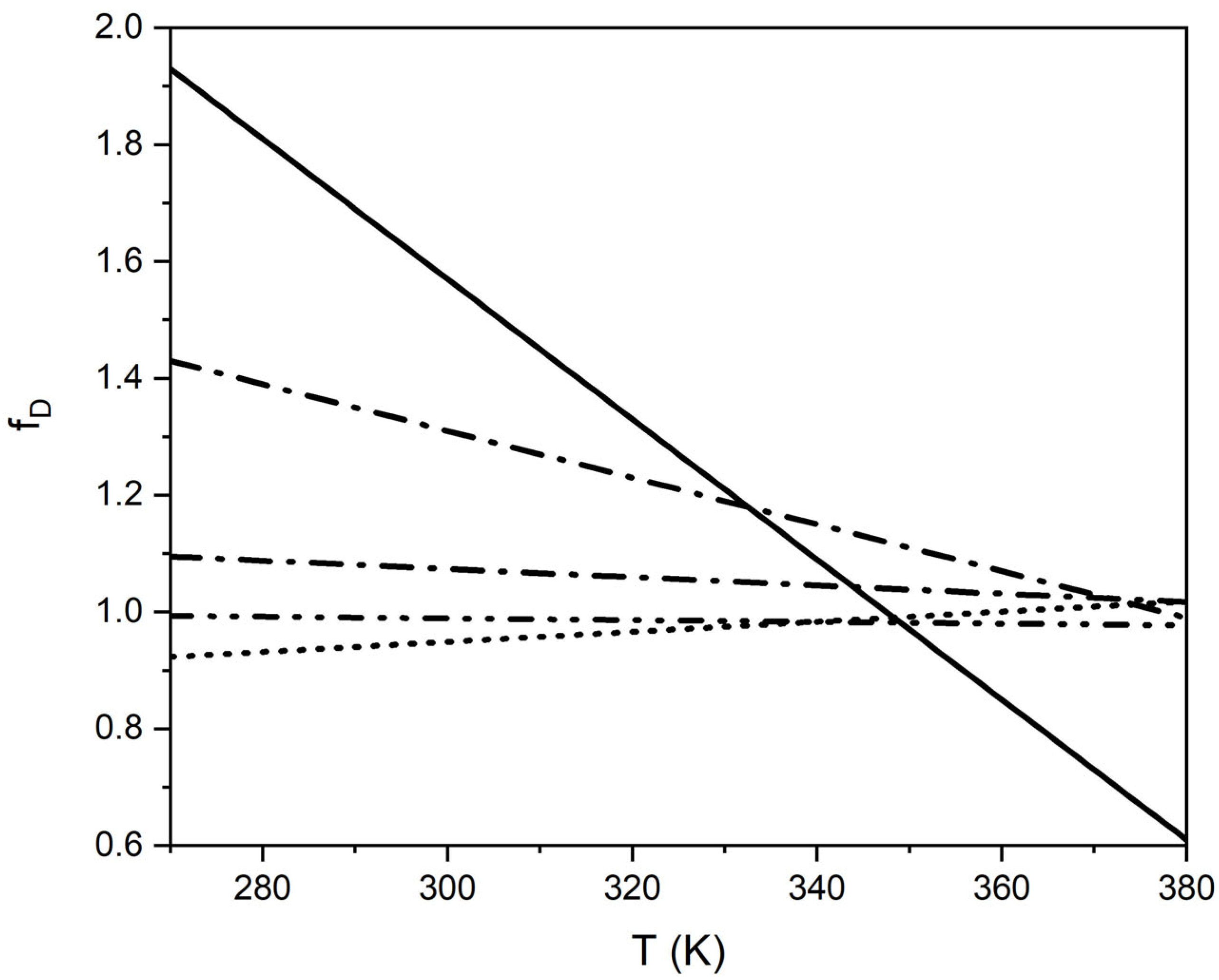
For n-alkanes [34,35], the following values for the factor fD = aD + bDT in Equation (25) were the result:
fD1 = 0.544 + 1.426 × 10⁻³·M + (5.5 × 10⁻⁴ + 2.483 × 10⁻⁶·M)·T for n = (M − 2)/14 ≤ 10 and
fD2 = 0.544 + 1.426 × 10⁻³·M + (1.26 × 10⁻³ − 2.374 × 10⁻⁶·M)·T for n ≥ 11
fD2 = 0.544 + 1.426 × 10⁻³·M + (1.26 × 10⁻³ − 2.374 × 10⁻⁶·M)·T for n ≥ 11
For a compound CnH2n+2 only the number n of carbon atoms and the temperature were needed.
For heptane the percentage average absolute deviation AAD% = 6.3 for 7 DL-values in the temperature range 190 < K < 377 [35]. For dodecane and tetradecane the corresponding errors were AAD% < 5 [34]. The error (e%) between experimental and predicted DL-values was 0.1 for octadecane at 50 °C and −16 for C32H66 at 100 °C [35].
An increase in the aD-values and decrease in the bD-values resulted in increasing polarities of the compounds (Figure 7). This behavior allowed for a rough estimation of the DL-values for compounds with unknown fD-values. With more experimental data, closer correlations between fD-values and functional groups are possible. A rough estimation of self-diffusion values is also possible from viscosity coefficients, as shown below in Section 4.8.
4.7.5. Binary Liquid Diffusion Coefficients
A binary mixture of n-hexane (A) and n-dodecane (B) was considered as an additional example of liquid diffusion. The mutual diffusion of these two hydrocarbons increases as the mixture becomes richer in A. If the mole fraction XA → 1.0, the mutual diffusion coefficient DAB = DBA → D°BA, where this notation signifies that the limiting diffusivity represents the diffusion of B in a medium consisting essentially of A [3]. Similarly, D°AB is the diffusivity of A in essentially pure B. Self-diffusion coefficients differ from binary-diffusion coefficients, and there is no way to relate the two coefficients directly, without an additional specific parameter [3].
Liquid state theories for calculating binary liquid diffusion coefficients are not satisfactory in providing relations for calculating the mutual diffusion coefficient DAB. Different models are presented in [3]. Some models are based on the Stokes–Einstein equation, which strictly applies to macroscopic systems with large spherical molecules diffusing in a dilute solution.
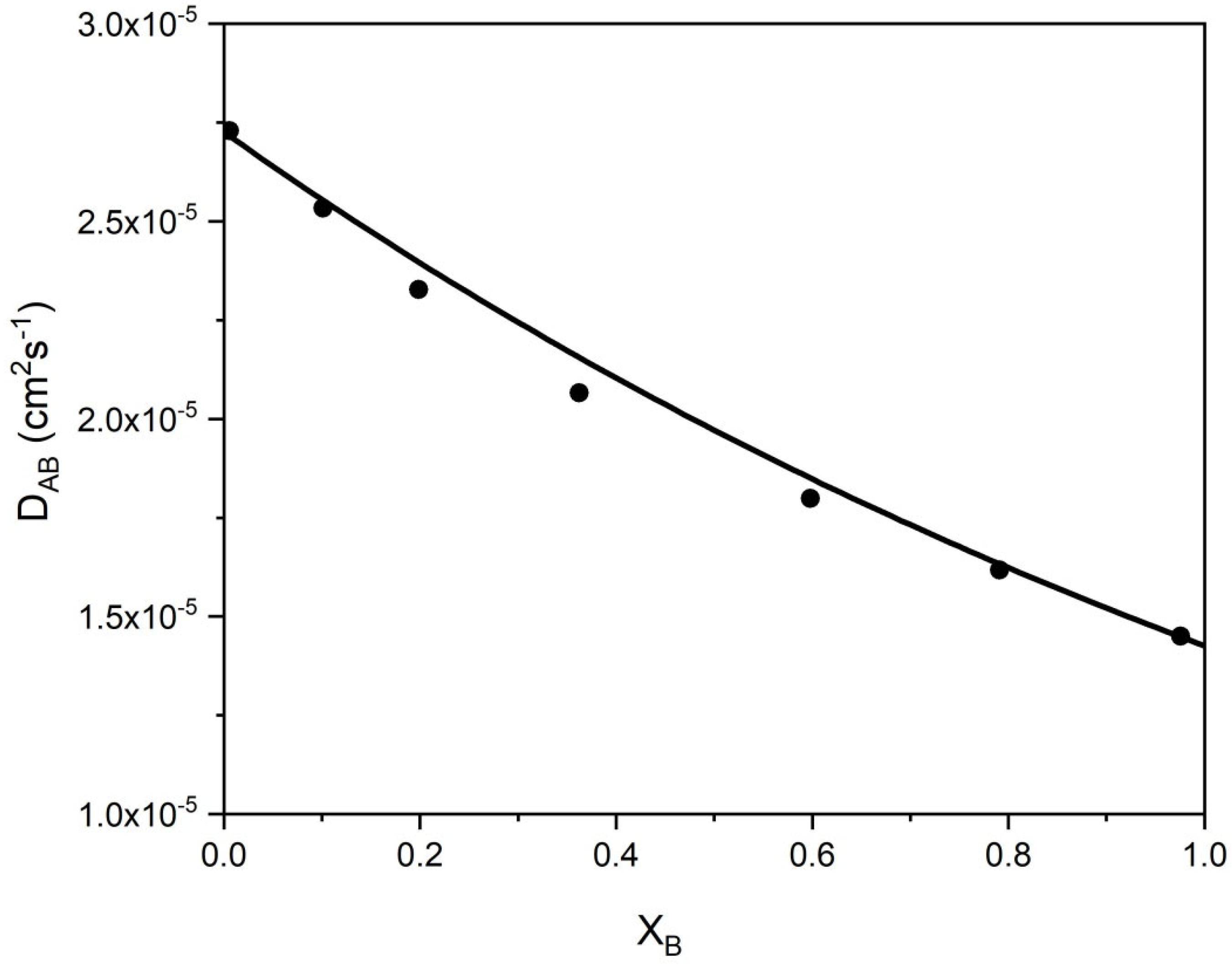
The following equation is proposed for the mutual diffusion coefficient in a binary mixture of compounds with the relative molecular masses MA and MB as function of the mole fraction XB:
where XA and XB are the mole fractions of A and B in the liquid, A = (MA − 2)/14 in wA,e = (1 + 2π/A)A/e, and B = (MB − 2)/14 in wB,e = (1 + 2π/B)B/e. The corresponding factors fDA and fDB are for the pure compounds A and B, respectively, introduced above for the self-diffusion coefficients.
δD is an interaction factor of the two compounds in the binary system that is obtained from a comparison of the calculated data using Equation (28) with a few experimental points.
If A = B, wB,e = wA,e, fDA = fDB = fD, XA = XB = 1, and δD = 0. That means that Equation (28) leads to Equation (25). For the binary system hexane(A)-dodecane(B), δD = 0.86·XA + 0.105. The AAD% = 1.6 for DAB at 298.15 K [35] (Figure 8).
For hexane(A)-hexadecane(B), δD = XA + 0.045.
For the binary system benzene (A)-ethanol (B) at 25 °C and Equation (28), the interaction factor δD is: δD25 = 1.8·XB (1 − XB)4 − 0.93·XB1.5 + 0.79.
δD40 = 1.55XB (1 − XB)4 − 0.89·XB1.6 + 0.77 at 40 °C and AAD% = 2.8.
4.7.6. Diffusion Coefficients in Liquids at Infinite Dilution
The following relation was defined for the diffusion coefficient D°AB of compound A at infinite dilution in a solvent of compound B:
In addition to the molecular weights of solvent B and solute A and factor fDB = aDB + bDBT for the self-diffusion of B, factor φB = c + d·wA,e is needed to predict the whole series of D°AB data in one solvent B. Factor φB with its linear dependence from wA,e resulted from comparisons of data calculated with Equation (29) along with a few experimental data and allowed for the easy determination of c and d from two known D°AB-values.
In Table 4 the experimental D°AB values for 6 compounds in decane are compared with the predicted values with Equation (29).
With φB,alk = −0.63 + 0.17·wB,e + (0.306 − 0.039·wB,e)·wA,e for n-alkanes, the AAD% values for the D°AB values calculated with Equation (29) for the six solutes in Table 4 at 25 °C in n-hexane, n-heptane, n-octane, and n-decane were 2.3, 2.9, 2.1, and 0.84, respectively, in comparison to the experimental values [10].
In Table 5 the D°AB values for 26 compounds in water and the errors from comparison with predicted values obtained with Equation (29) are listed.
4.8. Modeling Viscosities of Liquids Using the Interaction Function
There is no satisfactory theoretical basis available yet for the estimation of liquid viscosities [3]. However, a strong connection between viscosity and liquid diffusion coefficients exists [1]. In this model, the following equation for the prediction of the liquid viscosity coefficient is proposed:
where:
= 4.3621 × 10⁻⁴ Pa s and wn,e = (1 + 2π/n)n/e, where n = (Mn − 2)/14.
The viscosity reference factor results from the inverse value of the self-diffusion reference factor DL,r in Equation (26).
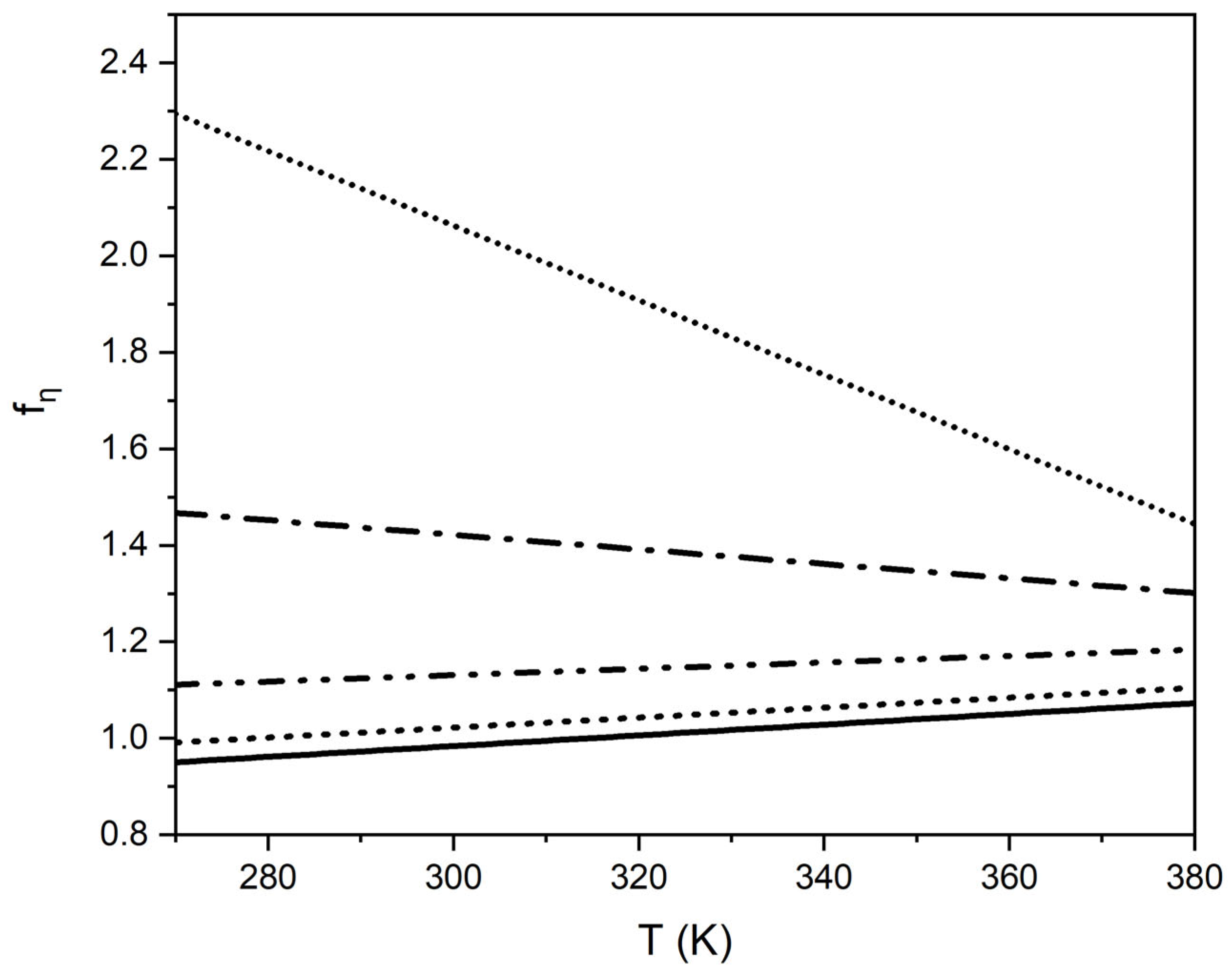
In the following, empirical factors fη = aη + bηT in Equation (30) obtained from fitting experimental data for a series of compounds and homologous series are given and the calculated viscosity coefficients are compared to the literature data [10] in the temperature range of −25 < t < 100 °C. Only the relative molecular mass M for n = (M − 2)/14 and the temperature T were needed.
For the n-alkanes:
fη = 0.38 + 0.0518·wn,e + (1.049 × 10⁻³ +6.364 × 10⁻⁷·M)·T.
For the homologous series of 1-alcohols with n > 3 (propanol):
fη = 2.685 − 0.18·wn,e + (0.0004·wn,e − 0.0031)T.
For the homologous series of carboxylic acids with n > 2 (acetic acid):
fη = 0.5 + 0.1·wn,e + (1.309 × 10⁻³ − 4.286 × 10⁻⁶ M)·T.
The AAD% values of the viscosities for liquid n-alkanes with n carbon atoms from hexane to hexadecane, calculated with Equations (30) and (31) in the temperature range of −25 < t °C < 100, were < 4. For pentane AAD% = 12.6 and for octadecane, AAD% = 9.
The AAD% values for the alcohols between −25 and 100 °C were 1.7–12 (mean 5.3).
The AAD% values for the carboxylic acids between 0 and 100 °C were 1.7–12.2 (mean 5.7).
The corresponding factors fη = aη + bη·T for several other compounds are shown in Table 6.
The fη values for alkylbenzenes, 2-ketones, and ethyl acetate between 25–50 °C were between 1.05 and 1.15. An increase in the aη-values and decrease in the bη-values resulted in increasing polarities of the compounds (Figure 10). This behavior is similar to that of the self-diffusion coefficients (Figure 7).
An important relation between the self-diffusion coefficient and the viscosity coefficient in a liquid is the product Θ:
Θ = DL·ηL·108.
The Θ-values lie near 1 and for many organic compounds one mean value Θ = 1.25 can be used. A few examples of the AAD% values for DL estimated with Equation (32) using the corresponding ηL data are shown in Table 7.
There are many experimental data for ηL values available in the literature for different structural groups [12]. From such collections the corresponding terms aη and bη can be easily determined. From aη and bη values for different structures, as exemplified in the above tables, estimates of DL-values are possible using Equation (32), for which no experimental data are available.
4.9. Modeling of Diffusion in Polymers Using the Interaction Function
The diffusion behavior of organic compounds solved in polymers lies between that of liquids and solids. As a consequence, the models for diffusion coefficient estimation are based on ideas drawn from diffusion in both liquids and solids [6].
The literature contains a very large amount of information on the diffusion of molecules in polymers [38]. The considerable interest and the academic and industrial research efforts in the study of diffusion in polymers arises from the fact that important practical applications for these materials depend to a great extent on diffusion phenomena.
In addition to microscopic molecular or free-volume models, atomistic computational approaches based on molecular dynamics play important roles. However, the many adjustable parameters needed for predictions of unknown diffusion coefficients are not known in many cases and it is often questionable whether such models are helpful for practicable applications.
With the aim to deliver an additional tool to assist in making material safety regulation decisions in the USA Food and Drug Administration (FDA) and in the European Union (EU), simple empirical models for the estimation of diffusion coefficients DP were proposed. In a first approximation, DP was correlated with the relative molecular mass M of the migrant and a matrix-specific (polymer) parameter AP at temperature T [39]. A similar approach was undertaken by the FDA [40].
Despite the fact that many sophisticated models for the prediction of diffusion coefficients in polymers are known, only the very simplified models as published in [39,40] were finally useful for regulation decisions. Further development of this simplified empirical approach delivered a useful tool for regulatory decisions by the FDA and EU [41].
Since 2000, a series of improvements on the model have been made [6]. From these developments the following model for the diffusion of organic molecules in polymers is now proposed.
Based on Equation (24) for solids and Equation (25) for liquids, the following general equation for diffusion constants Dp of a compound with the interaction function wn,e in a polymer, represented with the matrix value w, is proposed:
Polymethylene represents a reference polymer with the matrix value w and melting point TP,∞ = Tm,∞ = 416 K and fP = 1; wn = (1 + 2π/n)n/e, where n = (M − 2)/14 and the M is the relative molecular mass of the diffusing molecule.
For the general case, the empirical polymer specific constant fP takes into account the structure of the matrix and its variation with the temperature T in K. In contrast to the solid state, as for metals, the polymer matrix shows different degrees of rigidity. Between a glassy state at low temperatures and a thermoplastic state, the interaction with the diffusing particle changes. The consequence is a variable activation energy:
From the great variety of polymers, two well-known, extremely different types were selected: high-density polyethylene (HDPE) with a well-known melting temperature TP = 408 K (135 °C) and polyethylene terephthalate (PET) with TP = 528 K (255 °C). HDPE is thermoplastic in the temperature range for most applications, whereas PET is glassy at t < 70 °C.
Both polymers are very well studied and deliver reliable values needed for modeling. From experimental data for the diffusion coefficients of compounds up to M = 1500 in the temperature range of 23 < t < 100 °C for HDPE and 23 < t < 175 °C for PET, the corresponding fP-values for Equations (33) and (34) were determined. They show a linear behavior and are represented by the two following functions. For HDPE:
With these values the activation energies for diffusion in HDPE and PET are represented in Figure 11a as functions of M and in Figure 11b as functions of 1/T.
The behavior of the activation energy of diffusion in PET in conformity with Equations (34) and (35) is in good agreement with the experimental data from [42,43].
As an example, for diffusion modeling in HDPE in conformity with Equation (33), eight compounds with different structures used as additives in plastics with 100 < M < 1200 are listed in Table 8. Their diffusion coefficients DP in HDPE at 60 °C are shown in Figure 12.
For an unknown thermoplastic matrix, two experimental diffusion values for a compound with known M at two temperatures are needed for the determination of the linear function fP. For a glassy matrix in the interested temperature range, two additional measured diffusion values are needed in the glassy region.
The advantage of Equation (33) is the possibility of an easy prediction of diffusion coefficients over the whole mass and temperature range for a polymer, based on just two measured points for one compound with known M at two temperatures T.
To maintain the validity of Equation (33), the total concentrations of the diffusing components should remain below ≈5% in order to avoid softening the matrix, resulting in changes (increasing) to the diffusion rate. The same precaution must be taken for the contact media used when measuring the diffusion coefficient to avoid swelling of the polymer matrix. In order to take into account such influences, an additional parameter AP can be introduced into Equation (33), which must be determined experimentally with an additional measurement [6].
5. Conclusions
The interaction function in Equation (3) for liquid particles is based on the fundamental properties of natural numbers. This function acts as a bridge between properties of elementary particles and emergent properties of macroscopic systems. The atomic mass unit and an internal molar kinetic energy term for a system with optimal molar entropy are derived as two examples. This leads to a temperature T0 = 2.98 K in a macrosystem of particles with the atomic mass unit u and the molar entropy Sm = 108.85 JK−1mol−1. The same entropy value results for the system at a reference temperature Tr = 298.15 K and a pressure of 105 Pa. In such an environment, the maximum of structure variety, including life, is possible.
Even one organic molecule can be treated as a system of i interacting subparticles in conformity with the interaction function defined in Equation (3). The non polar Methylene group -CH2- with two strong covalent bonded H-atoms is such a subparticle, with a certain individuality along the i carbon atoms in a chain. The property of chain formation is characteristic for organic compounds and the n-alkanes are therefore the reference series for all organic compounds.
A variety of physical properties of liquids is described on the basis of the interaction function. All corresponding specific values for constants are based on Equation (3).
The important conclusion is the possibility to predict values for specific properties of liquids, starting from an uniform point of view, with the interaction function wn,e using a minimum of empirical constants as simple, essentially linear temperature functions in addition to the molecular mass M.
The correlation of the power sequence in Equation (3) with the homologous series of n-alkanes as a reference for all organic compounds is one main basis. All specific structure properties can be covered with additional empirical increments with the same dimensionless units as M. This allows, in theory, for the creation of corresponding maps of such structure increments for all important functional groups, similar to charts of infrared spectra, as an example. Such data can then be easily used by introducing them directly into the prediction equations.
The correlation of emergent properties of fluid systems with the interaction function in Equation (3) provides a reliable basis for applications with a minimum of empirical data and computational effort. That way it offers an attractive alternative to many sophisticated prediction methods. Practical applications for diffusion modeling in plastic materials for food and pharmaceutical packaging and for modeling interactions with the environment are typical examples of the usefulness of such simple approaches. The interaction function represents the real basic phenomenon of the liquid state, in contrast to all models starting alone from pair interactions.
Funding
This research received no external funding.
Institutional Review Board Statement
Not applicable.
Informed Consent Statement
Not applicable.
Data Availability Statement
Not applicable.
Acknowledgments
The author would like to thank Albert L. Baner for helpful discussions about the content and structure of this study.
Conflicts of Interest
The author declares no conflict of interest.
References
- Hirschfelder, J.O.; Curtiss, C.F.; Bird, R.B. Molecular Theory of Gases and Liquids; John Wiley & Sons, Inc.: New York, NY, USA, 1954. [Google Scholar]
- Sadus, R.J. Exact calculation of the effect of three-body Axilrod-Teller interactions on vapour-liquid phase coexistence. Fluid Phase Equilib. 1998, 144, 351–360. [Google Scholar] [CrossRef]
- Poling, B.E.; Prausnitz, J.M.; O’Connell, J.P. The Properties of Gases and Liquids, 5th ed.; McGRAW-Hill: New York, NY, USA, 2001. [Google Scholar]
- Courant, R.; Robbins, H. What Is Mathematics, 2nd ed.; Oxford University Press: Oxford, UK, 1996. [Google Scholar]
- Piringer, O.G. A predictive power sequence equation for vapour pressures of pure organic fluids and partial pressures in multicomponent systems in equilibrium. Fluid Phase Equilib. 2020, 506, 112409. [Google Scholar] [CrossRef]
- Piringer, O.G. A uniform model for prediction of diffusion coefficients with emphasis on plastic materials. In Plastic Packaging: Interactions with Food and Pharmaceuticals; Piringer, O.G., Baner, A.L., Eds.; Wiley-VCH: Weinheim, Germany, 2008; p. 163. [Google Scholar]
- Atkins, P.; de Paula, J. Physical Chemistry, 8th ed.; Oxford University Press: Oxford, UK, 2006. [Google Scholar]
- Pauling, L. General Chemistry, 3rd ed.; W.H.Freeman & Co.: San Francisco, CA, USA, 1970. [Google Scholar]
- Hagemann, J.W.; Rothfus, J.A. Computer modelling for stabilities and structure relation-ships of n-hydrocarbons. J. Am. Oil Chem. Soc. 1979, 56, 1008–1013. [Google Scholar] [CrossRef]
- Lide, D.R. (Ed.) Handbook of Chemistry and Physics, 89th ed.; Sections 3 and 6; Taylor & Francis Group: Abingdon, UK; CRC Press: Boca Raton, FL, USA, 2004. [Google Scholar]
- Stack, G.M.; Mandelkern, L.; Kröhnke, C.; Wegner, G. Melting and crystallisation kinetics of a high molecular weight n-alkane: C192H386. Macromolecules 1989, 22, 4351–4361. [Google Scholar] [CrossRef]
- DIPPR 801 Tables; Thermophysical Properties Database: 2018.
- Höhne, G.W.H. Another approach to the Gibbs-Thomson equation and the melting point of polymers and oligomers. Polymer 2002, 43, 4689–4698. [Google Scholar] [CrossRef]
- Lee, K.S.; Wegner, G. Linear and cyclic alkanes (CnH2n+2, CnH2n) with n > 100. Synthesis and evidence for chain-folding. Die Makromol. Chem. Rapid Commun. 1985, 6, 203–208. [Google Scholar] [CrossRef]
- Holleman, A.F.; Wiberg, E.; Wiberg, N. Lehrbuch der Anorganischen Chemie; Walter de Gruyter: Berlin, Germany; Auflage: New York, NY, USA, 2007; p. 2002. [Google Scholar]
- Buffat, P.H.; Borel, J.-P. Size effect on the melting temperature of gold particles. Phys. Rev. A 1976, 13, 2287–2298. [Google Scholar] [CrossRef] [Green Version]
- Ercolessi, F.; Andreoni, W.; Tosatti, E. Melting of small gold particles: Mechanism and size effects. Phys. Rev. Lett. 1991, 66, 911–914. [Google Scholar] [CrossRef] [PubMed]
- Cleveland, C.L.; Luedtke, W.D.; Landman, U. Melting of gold clusters: Icosahedral precursors. Phys. Rev. Lett. 1998, 8, 2036–2039. [Google Scholar] [CrossRef] [Green Version]
- Zhang, M.; Efremov, M.Y.; Schiettekatte, F.; Olson, E.A.; Kwan, A.T.; Lai, S.L.; Wisleder, T.; Greene, J.E.; Allen, L.H. Size-dependents melting point depression of nanostructures: Nanocalorimetric measurements. Phys. Rev. B 2000, 62, 10548–10557. [Google Scholar] [CrossRef] [Green Version]
- Coombes, C.J. The melting of small particles of lead and indium. J. Phys. F Met. Phys. 1972, 2, 441–449. [Google Scholar] [CrossRef]
- David, T.B.; Lereah, Y.; Deutscher, G.; Kofman, R.; Cheyssac, P. Solid-liquid transition in ultra-fine lead particles. Philos. Mag. A 1995, 71, 1135–1143. [Google Scholar] [CrossRef]
- Lai, S.L.; Guo, J.Y.; Petrova, V.; Ramanath, G.; Allen, L.H. Size-dependent melting properties of small tin particles: Nanocalorimetric measurements. Phys. Rev. Lett. 1996, 77, 99–102. [Google Scholar] [CrossRef] [PubMed] [Green Version]
- SLai, L.; Carlsson, J.R.A.; Allen, L.H. Melting point depression of Al clusters generated during the early stages of film growth: Nanocalorimetric measurements. Appl. Phys. Lett. 1998, 72, 1098–1100. [Google Scholar]
- Chushak, Y.G.; Bartell, L.S. Melting and Freezing of Gold Nanoclusters. J. Phys. Chem. B 2001, 105, 11605–11614. [Google Scholar] [CrossRef]
- Safaei, A.; Shandiz, M.A.; Sanjabi, S.; Barber, Z.H. Modeling the Melting Temperature of Nanoparticles by an Analytical Approach. J. Phys. Chem. C 2008, 112, 99–105. [Google Scholar] [CrossRef]
- Qi, W.H.; Wang, M.P.; Zhou, M.; Shen, X.Q.; Zhang, X.F. Modeling cohesive energy, and melting temperature of nanocrystals. J. Phys. Chem. Solids 2006, 67, 851–855. [Google Scholar] [CrossRef]
- Findenegg, G.H.; Jähnert, S.; Akcakayiran, D.; Schreiber, A. Freezing and melting of water confined in silica. ChemPhysChem 2008, 9, 2651–2659. [Google Scholar] [CrossRef] [PubMed]
- Schreiber, A.; Ketelsen, I.; Findenegg, G.H. Melting and freezing of water in ordered mesoporous silica materials. Phys. Chem. Chem. Phys. 2001, 3, 1185–1195. [Google Scholar] [CrossRef]
- Jähnert, S.; Chavez, F.V.; Schaumann, G.E.; Schreiber, A.; Schönhoff, M.; Findenegg, G.H. Melting and freezing of water in cylindrical silica nanopores. Phys. Chem. Chem. Phys. 2008, 10, 6039–6051. [Google Scholar] [CrossRef] [Green Version]
- Factorovich, M.H.; Molinero, V.; Scherlis, D.A. Vapor pressure of water nanoparticles. J. Am. Chem. Soc. 2014, 136, 4508–4514. [Google Scholar] [CrossRef]
- Kestin, J.; Knierim, K.; Mason, E.A.; Najafi, B.; Ro, S.T.; Waldman, M. Equilibrium and transport properties of the noble gases and their mixtures at low density. J. Phys. Chem. Ref. Data 1984, 13, 229–303. [Google Scholar] [CrossRef]
- Cussler, E.L. Diffusion: Mass Transfer in Fluid Systems, 2nd ed.; Cambridge University Press: Cambridge, UK, 1997. [Google Scholar]
- Mehrer, H.; Stolica, N.; Stolwuk, N.A. Landolt-Börnstein, Numerical data and functional relationships in science and technology, new series. In Self-Diffusion in Solid Metallic Elements; Mehrer, H., Ed.; Diffusion in solid metals and alloys; Springer: Berlin/Heidelberg, Germany, 1991; Volume 26. [Google Scholar]
- Holz, M.; Heil, S.R.; Sacco, A. Temperature-dependent self-diffusion coefficients of water and six selected molecular liquids for calibration in accurate 1H NMR PEG measurements. Phys. Chem. Chem. Phys. 2000, 2, 4740–4742. [Google Scholar] [CrossRef]
- Andrussow, L.; Schramm, B. (Eds.) Landolt-Börnstein, Zahlenwerte und Funktionen, II-Band, 5b.Teil; Diffusion in Flüssigkeiten; Springer: Berlin/Heidelberg, Germany, 1969. [Google Scholar]
- Bosse, D.; Bart, H.-J. Prediction of Diffusion Coefficients in Liquid Systems. Ind. Eng. Chem. Res. 2006, 45, 1822–1828. [Google Scholar] [CrossRef]
- Anderson, D.K.; Hall, J.R.; Babb, A.L. Mutual Diffusion in Non-Ideal Binary Liquid Mixtures. J. Phys. Chem. 1958, 62, 404–408. [Google Scholar] [CrossRef]
- Mercea, V. Models for diffusion in polymers, in Plastic Packaging. In Interactions with Food and Pharmaceuticals; Piringer, O.G., Baner, A.L., Eds.; Wiley-VCH: Weinheim, Germany, 2008; p. 123. [Google Scholar]
- Piringer, O. Evaluation of plastics for food packaging. Food Add. Contam. 1994, 11, 221–230. [Google Scholar] [CrossRef] [PubMed]
- Limm, W.; Hollifield, H.C. Modelling of additive diffusion in polyolefines. Food Add. Contam. 1996, 13, 949–967. [Google Scholar] [CrossRef] [PubMed]
- Begley, T.; Castle, L.; Feigenbaum, A.; Franz, R.; Hinrichs, K.; Lickly, T.; Mercea, P.; Milana, M.; O’Brien, A.; Rebre, S.; et al. Evaluation of migration models that might be used in support of regulations for food-contact plastics. Food Add. Contam. 2005, 22, 73–90. [Google Scholar] [CrossRef] [PubMed] [Green Version]
- Ewender, J.; Welle, F. Determination and prediction of the lag times of hydrocarbons through a polyethylene terephthalate film. Packag. Technol. Sci. 2014, 27, 963–974. [Google Scholar] [CrossRef]
- Welle, F.; Franz, R. Diffusion coefficients and activation eneegies of diffusion of low molecular weight migrants in polyethyleneterephthalate bottles. Polym. Test. 2012, 31, 93–101. [Google Scholar] [CrossRef]
- Mercea, P.V.; Kalisch, A.; Ulrich, M.; Benz, H.; Piringer, O.G.; Tosa, V.; Schuster, R.; Aranyi, S.; Sejersen, P. Modelling migration of substances fro polymers into drinking water. Part 1-Diffusion coefficient estimations. Polym. Test. 2018, 65, 176–188. [Google Scholar]
Figure 1.
Graph of the function y = x2π/x.

Figure 2.
Experimental data [16] (x) and calculated melting temperatures of different diameter d gold clusters. The solid line represents Equation (9) and the dashed line represents n = a·d/d0 in Equation (9).
Figure 2.
Experimental data [16] (x) and calculated melting temperatures of different diameter d gold clusters. The solid line represents Equation (9) and the dashed line represents n = a·d/d0 in Equation (9).

Figure 3.
Experimental [28] freezing temperatures (▼), melting temperatures (★), and calculated (—) transition temperatures per Equation (12) as a function of the pore diameter.
Figure 3.
Experimental [28] freezing temperatures (▼), melting temperatures (★), and calculated (—) transition temperatures per Equation (12) as a function of the pore diameter.

Figure 4.
Predicted vapor mole fractions Y1 (. . . .) of n-heptane and Y2 (- - - -) for toluene in the binary system n-heptane(1)-toluene(2) at 25 °C [5] in comparison with experimental values (●) and (▲).
Figure 4.
Predicted vapor mole fractions Y1 (. . . .) of n-heptane and Y2 (- - - -) for toluene in the binary system n-heptane(1)-toluene(2) at 25 °C [5] in comparison with experimental values (●) and (▲).

Figure 5.
Comparison of the ln(P/P*) results obtained in the Hg droplet radius range of 1 nm ≤ r ≤ 10 nm with (—) Equation (19), where k = 1, fv = 1.062, and (●) the Kelvin Equation (20) atö 25 °C.
Figure 5.
Comparison of the ln(P/P*) results obtained in the Hg droplet radius range of 1 nm ≤ r ≤ 10 nm with (—) Equation (19), where k = 1, fv = 1.062, and (●) the Kelvin Equation (20) atö 25 °C.

Figure 6.
Logarithm of the relative vapor pressure of water nanodroplets ln(P/P*) as a function of the inverse radius r (nm) at temperature 298 K. The corresponding experimental values (●) from [30], compared to the values (- - - -) calculated with the Kelvin Equation (20) and (—) with the interaction function in Equation (19).

Figure 7.
The factors fD = aD + bDT in Equation (25) for the self-diffusion of 5 compounds as a function of temperature T K. From bottom to the top at low temperatures: n-heptane, ethyl-acetate, benzene, methanol, water.
Figure 7.
The factors fD = aD + bDT in Equation (25) for the self-diffusion of 5 compounds as a function of temperature T K. From bottom to the top at low temperatures: n-heptane, ethyl-acetate, benzene, methanol, water.

Figure 8.
Diffusion coefficients DAB in a binary system hexane (A)-hexadecane (B) at 25 °C with experimental points (●) [35] and calculated (—) with Equation (28).
Figure 8.
Diffusion coefficients DAB in a binary system hexane (A)-hexadecane (B) at 25 °C with experimental points (●) [35] and calculated (—) with Equation (28).

Figure 9.
Diffusion coefficients DAB in a binary system of benzene (A)-ethanol (B) at 25 °C with experimental (●) [35] and calculated (---) values with Equation (28), and at 40 °C with experimental (♦) [35] and calculated (…) values with Equation (28).

Figure 10.
The factors fη = aη + bη·T in Equation (30) of 5 compounds as a function of temperature T K. From bottom to the top at low temperatures: n-heptane, ethyl-acetate, benzene, methanol, water.
Figure 10.
The factors fη = aη + bη·T in Equation (30) of 5 compounds as a function of temperature T K. From bottom to the top at low temperatures: n-heptane, ethyl-acetate, benzene, methanol, water.

Figure 11.
(a) Activation energy of diffusion in polymers as a function of the relative molecular mass M. (—) ED in HDPE with fHDPE; (. . .) ED in thermoplastic PET; (- - -) ED in glassy PET with the corresponding fP-values from Equation (35). (b) The product TP,∞·fP from Equation (34) as function of 1/T. (—) TP,∞·1; (3) TP,∞· from Equation (35); (1) TP,∞·; (2) TP,∞· from Equation (35).


Figure 12.
Diffusion coefficients in HDPE at 60 °C. (●) Compounds from Table 8 [44]; (▼) n-alkanes with 20, 27, 32 and 40 carbon atoms [6]; (■) water [5].

Table 1.
Difference ΔTcalc-exp K between melting points Tm,calc calculated with Equation (6) and available experimental values Tm,exp for n-alkanes with i > 23 carbon atoms.
Table 1.
Difference ΔTcalc-exp K between melting points Tm,calc calculated with Equation (6) and available experimental values Tm,exp for n-alkanes with i > 23 carbon atoms.
| i | ΔTcalc-exp | Ref. | i | ΔTcalc-exp | Ref. |
|---|---|---|---|---|---|
| 24 | 0.23 | [12] | 35 | −0.34 | [10] |
| 25 | 0.10 | [12] | 36 | −0.09 | [12] |
| 26 | 0.11 | [12] | 38 | 0.11 | [10] |
| 27 | −0.33 | [12] | 40 | −0.13 | [10] |
| 28 | −0.21 | [12] | 44 | 0.48 | [10] |
| 29 | −0.51 | [12] | 46 | 0.57 | [10] |
| 30 | −0.22 | [12] | 50 | −0.17 | [10] |
| 32 | −0.06 | [12] | 60 | 0.09 | [10] |
| 34 | 0.13 | [10] | 192 | 0.44 | [11] |
Table 2.
The densities ρ (g/cm3), molar volumes Vm (m3/mol), and surface tensions γ (N/m) at 5 temperatures for Hg, where Tm = 234.316 K and M = 200.59 (g/mol) [10].
Table 2.
The densities ρ (g/cm3), molar volumes Vm (m3/mol), and surface tensions γ (N/m) at 5 temperatures for Hg, where Tm = 234.316 K and M = 200.59 (g/mol) [10].
| t °C | 10 | 25 | 50 | 75 | 100 |
|---|---|---|---|---|---|
| ρ | 13.57043 | 13.53359 | 13.47251 | 13.41181 | 13.35142 |
| Vm 105 | 1.478 | 1.482 | 1.4889 | 1.4956 | 1.502 |
| γ | 0.48855 | 0.48548 | 0.48036 | 0.47523 | 0.47011 |
| i | 55.467 | 55.417 | 55.334 | 55.250 | 55.167 |
| ln(P/P*) | 0.613 | 0.580 | 0.532 | 0.491 | 0.455 |
| w − wA,i | 0.614 | 0.580 | 0.547 | 0.487 | 0.456 |
| e% | −0.16 | 0.0 | −2.82 | 0.815 | −0.22 |
e = 100·(ln(P/P*) − (w − wA,i))/ln(P/P*).
Table 3.
The aD and bD values for the factor fD in Equation (25) and the AAD% values for N measured DD-values in the temperature range ΔT [34] b, [35] a for 13 compounds.
| Compound | aD | bD·103 | AAD% | N | ΔT (°C) |
|---|---|---|---|---|---|
| Methylacetate a | 0.928 | 0.1933 | 0.1 | 4 | 15–45 |
| Ethylacetate a | 1.034 | −0.15 | 1.9 | 5 | 15–55 |
| Dioxane b | 1.1666 | 0.05 | 0.4 | 5 | 15–55 |
| Cyclopentane a | 1.22 | −0.6751 | 6.4 | 4 | −23–46 |
| Cyclohexane b | 1.1934 | −0.1752 | 0.4 | 5 | 15–55 |
| Benzene a | 1.285 | −0.7045 | 4.2 | 12 | 7–65 |
| DMSO b | 1.3646 | −0.633 | 0.3 | 4 | 25–55 |
| 1- Pentanol b | 2.056 | −2.0 | 1.0 | 6 | 5–55 |
| 1-Butanol a | 1.8337 | −1.365 | 0.1 | 3 | 25–45 |
| 1-Propanol a | 1.992 | −1.733 | 0.4 | 4 | 15–45 |
| Ethanol a | 2.66 | −3.952 | 1.4 | 8 | 7–65 |
| Methanol a | 2.51 | −4.0 | 2.0 | 8 | −5–55 |
| Water a | 5.17 | −12.0 | 4.1 | 21 | 0–100 |
Table 4.
Comparison of the D°AB-values for compounds with the relative molecular mass MA, calculated with Equation (29) with experimental data from [10]. Solvent n-decane, MB = 142 at 25 °C.
Table 4.
Comparison of the D°AB-values for compounds with the relative molecular mass MA, calculated with Equation (29) with experimental data from [10]. Solvent n-decane, MB = 142 at 25 °C.
| Compound | MA | D°AB·105 cm2s−1 (a) | e% |
|---|---|---|---|
| Benzene | 78.112 | 2.16 | −0.02 |
| Toluene | 92.138 | 1.93 | 1.81 |
| Ethylbenzene | 106.165 | 1.79 | 1.03 |
| Naphthalene | 128.174 | 1.65 | −2.0 |
| Pyrene | 202.25 | 1.23 | −0.07 |
| Perylene | 252.309 | 1.08 | 0.08 |
φB = 0.385 + 0.073·wA,e; (a) [10]; e% = 100 (DL,calc − DL,exp)/DL,exp.
Table 5.
D°AB-values in water. Compounds with relative molecular mass MA, experimental D°AB-values [10] at temperature T, and percent errors of the predicted D°AB-values.
Table 5.
D°AB-values in water. Compounds with relative molecular mass MA, experimental D°AB-values [10] at temperature T, and percent errors of the predicted D°AB-values.
| Compound | MA | D°AB·105 cm2s−1 | T (°C) | e% |
|---|---|---|---|---|
| Acetic acid | 60.05 | 1.29 | 25 | −7.8 |
| Acetone | 58 | 1.28 | 25 | −5.7 |
| Allyl alcohol | 58.08 | 0.90 | 15 | 4.3 |
| Aniline | 93.13 | 0.92 | 20 | −7.4 |
| DL-Arabinose | 150.13 | 0.69 | 20 | −1.0 |
| Benzene | 78 | 1.02 | 20 | −9.1 |
| Caprolactam | 113.16 | 0.87 | 25 | 5.5 |
| Cyclohexane | 84 | 0.84 | 20 | 6.5 |
| Diethylamine | 73.14 | 0.97 | 20 | −1.5 |
| 1,2-Ethanediol | 62 | 1.16 | 25 | 1.2 |
| Ethanol | 46 | 1.24 | 25 | 7.4 |
| Ethanolamin | 61.08 | 1.08 | 25 | 9.4 |
| Ethylbenzene | 106.1 | 0.81 | 20 | −1.1 |
| Ethyl carbamate | 89.09 | 0.80 | 15 | −6.8 |
| Glycerol | 92.09 | 1.06 | 25 | −5.9 |
| Glycine | 75 | 1.05 | 25 | 3.3 |
| D-Lactose | 342.3 | 0.38 | 15 | 0.43 |
| D-Mannitol | 182.17 | 0.50 | 15 | 2.1 |
| Methanol | 32 | 1.28 | 15 | 0.26 |
| 3-Methyl-1-butanol | 88 | 0.69 | 10 | −7.3 |
| Methylcyclopentane | 84 | 0.85 | 20 | 5.3 |
| Phenol | 94 | 0.89 | 20 | −4.7 |
| 1-Propanol | 60 | 0.87 | 15 | 6.0 |
| Propene | 42 | 1.44 | 25 | −3.9 |
| Raffinose | 504.42 | 0.33 | 15 | 0.07 |
| Toluene | 92 | 0.85 | 20 | 0.82 |
φB = 0.43 + 0.073wA,e; e% = 100(DL,calc − DL,exp)/DL,exp. AAD% = 4.4 (N = 26).
Table 6.
The aη and bη values for the compounds with relative molecular masses M and the AAD% from a comparison of the calculated viscosity coefficients to the literature data [10] for N measurements in the temperature range of −25 < t < 100 °C.
Table 6.
The aη and bη values for the compounds with relative molecular masses M and the AAD% from a comparison of the calculated viscosity coefficients to the literature data [10] for N measurements in the temperature range of −25 < t < 100 °C.
| Compound | aη | bη·103 | AAD% | N | M |
|---|---|---|---|---|---|
| Cyclohexane | 1.0402 | 0.51 | 5.0 | 4 | 84.161 |
| Benzene | 0.932 | 0.663 | 2.5 | 3 | 78.112 |
| Toluene | 0.736 | 1.112 | 0.3 | 6 | 92.138 |
| Ethylbenzene | 0.667 | 1.302 | 2.0 | 4 | 106.165 |
| Butylbenzene | 0.681 | 1.284 | 0.1 | 4 | 134.218 |
| Acetone | 0.794 | 0.8147 | 1.9 | 5 | 58.079 |
| 2-Butanone | 0.746 | 1.031 | 6.4 | 5 | 72.106 |
| 2-Pentanone | 0.721 | 1.105 | 4.2 | 12 | 86.132 |
| 2-Hexanone | 0.763 | 0.9768 | 0.1 | 3 | 100.159 |
| 2-Heptanone | 1.07 | 0.064 | 0.4 | 4 | 114.185 |
| Ethylacetate | 0.7123 | 1.033 | 1.4 | 8 | 88.106 |
| Formic acid | 1.82 | −0.5867 | 2.0 | 8 | 46.026 |
| Acetic acid | 1.134 | 0.8133 | 4.1 | 21 | 60.052 |
| Methanol | 1.875 | −1.51 | 0.2 | 3 | 32.042 |
| Ethanol | 1.89 | −1.28 | 0.6 | 5 | 46.068 |
| 1-Propanol | 2.025 | −1.625 | 1.0 | 5 | 60.095 |
| Water | 4.38 | −7.725 | 5.1 | 5 | 18.015 |
Table 7.
Comparison of self-diffusion coefficients DL,Θ = 1.25/ηL·108, DL,c calculated with Equation (25) and experimental values, and DL,ex for 4 organic compounds with different polarities from N data in the temperature range ΔT. For water, 21 data with DL,Θ = 2.2/ηL·108 are given.
Table 7.
Comparison of self-diffusion coefficients DL,Θ = 1.25/ηL·108, DL,c calculated with Equation (25) and experimental values, and DL,ex for 4 organic compounds with different polarities from N data in the temperature range ΔT. For water, 21 data with DL,Θ = 2.2/ηL·108 are given.
| Compound | DL,Θ − DL,ex (AAD%) | DL,c − DL,ex (AAD%) | N | ΔT (°C) |
|---|---|---|---|---|
| n-heptane | 9.8 | 8.3 | 5 | −46–104 |
| ethylacetate | 5.9 | 1.9 | 5 | 15–55 |
| benzene | 12 | 4.6 | 7 | 7–65 |
| methanol | 7.5 | 1.8 | 8 | −5–55 |
| H2O | 10.2 | 4.1 | 21 | 0–100 |
Table 8.
Additives with relative molecular masses M used in HDPE and their diffusion coefficients represented in Figure 12 [44].
| Migrant | M |
|---|---|
| 4-tert-Butylphenol | 150.22 |
| 2,4-Di-tert-butylphenol | 206.17 |
| 2,6-Di-tert-butyl-4-methylphenol | 220.6 |
| 3,5-Di-tert-butyl-4-hydroxybenzaldehyde | 234.16 |
| 3-(3,5-Di-tert-butyl-4-hydroxypheyl)-methylpropionate | 292.42 |
| Octaethyl-3-(3,5-di-tert-butyl-4-hydroxyphenyl)propionate | 530.88 |
| 1,3,5-Trimethyl-2,4,6-tris(3,5-di-tert-utyl-4-hydroxybenzyl)benzene | 775.22 |
| Pentaerythritol tetrakis[3-(3,5-i-tert-butyl-4-hydroxyphenyl)propionate] | 1177.67 |
Publisher’s Note: MDPI stays neutral with regard to jurisdictional claims in published maps and institutional affiliations. |
© 2021 by the author. Licensee MDPI, Basel, Switzerland. This article is an open access article distributed under the terms and conditions of the Creative Commons Attribution (CC BY) license (https://creativecommons.org/licenses/by/4.0/).
Share and Cite
MDPI and ACS Style
Piringer, O.G. A Power Sequence Interaction Function for Liquid Phase Particles. Fluids 2021, 6, 354. https://doi.org/10.3390/fluids6100354
AMA Style
Piringer OG. A Power Sequence Interaction Function for Liquid Phase Particles. Fluids. 2021; 6(10):354. https://doi.org/10.3390/fluids6100354
Chicago/Turabian StylePiringer, Otto G. 2021. "A Power Sequence Interaction Function for Liquid Phase Particles" Fluids 6, no. 10: 354. https://doi.org/10.3390/fluids6100354