Turbulence Model Assessment in Compressible Flows around Complex Geometries with Unstructured Grids


High Performance Computing and Visualization Laboratory, Department of Mechanical Engineering, University of Puerto Rico, Mayaguez, PR 00681, USA
Fluids 2019, 4(2), 81; https://doi.org/10.3390/fluids4020081
Submission received: 23 February 2019
/
Revised: 7 April 2019
/
Accepted: 15 April 2019
/
Published: 28 April 2019
(This article belongs to the Special Issue Multiscale Turbulent Transport)
Abstract
:One of the key factors in simulating realistic wall-bounded flows at high Reynolds numbers is the selection of an appropriate turbulence model for the steady Reynolds Averaged Navier–Stokes equations (RANS) equations. In this investigation, the performance of several turbulence models was explored for the simulation of steady, compressible, turbulent flow on complex geometries (concave and convex surface curvatures) and unstructured grids. The turbulence models considered were the Spalart–Allmaras model, the Wilcox k- model and the Menter shear stress transport (SST) model. The FLITE3D flow solver was employed, which utilizes a stabilized finite volume method with discontinuity capturing. A numerical benchmarking of the different models was performed for classical Computational Fluid Dynamic (CFD) cases, such as supersonic flow over an isothermal flat plate, transonic flow over the RAE2822 airfoil, the ONERA M6 wing and a generic F15 aircraft configuration. Validation was performed by means of available experimental data from the literature as well as high spatial/temporal resolution Direct Numerical Simulation (DNS). For attached or mildly separated flows, the performance of all turbulence models was consistent. However, the contrary was observed in separated flows with recirculation zones. Particularly, the Menter SST model showed the best compromise between accurately describing the physics of the flow and numerical stability.
1. Introduction
Wall-bounded turbulent flows at high Reynolds numbers are mainly characterized by a wide range of time and length scales (Pope [1]). In Direct Numerical Simulation (DNS), the full Navier–Stokes (NS) equations are generally solved to capture all time scales and eddies in the flow. This is an accurate approach that supplies extensive information, but it demands the use of a very fine mesh, and significant computational resources, to properly capture features in the order of the Kolmogorov scales [2]. Filtered Navier–Stokes equations, with an additional sub-grid scale stress term, are employed in Large Eddy Simulation (LES), in which large scales or eddies are directly resolved and the effects of the small scales are modeled [3]. The LES approach still requires high mesh resolution in boundary layer flows, particularly, in the near-wall region. Furthermore, the use of hybrid approaches (RANS-LES) to overcome the fine resolution needed in wall-bounded flows is an emerging and promising area [4]; nevertheless, there is still much ground to cover for industrial applications. From the perspective of performing turbulent industrial flow simulations, the workhorse is still the use of the Reynolds Averaged Navier–Stokes equations (RANS), which are obtained by time averaging the full NS equations. In this approach, almost the full power spectra of velocity fluctuations and turbulent kinetic energy are modeled, while capturing the very large turbulent scales of low frequencies. These equations require a model or closure to compute the Reynolds stresses, which arise from the convective terms of the NS equations after applying the time averaging process. The selection of an appropriate turbulence model is crucial to accurately represent important physical aspects of the flow, such as boundary layer separation and shock–boundary layer interaction [5]. Catalano and Amato [5] tested five different turbulence models in 2D and 3D classical aerodynamic applications: Spalart–Allmaras, Myong and Kasagi k-, Wilcox k-, Kok turbulent/non-turbulent (TNT), and Menter SST, where k is the turbulent kinetic energy, is the turbulent dissipation and is the specific rate of dissipation. They concluded that the Menter shear stress transport (SST) model exhibited the best balance between the physical capabilities and the numerical robustness for the transonic and high-lift flows explored. Knight et al. [6] performed a review of recent CFD simulations of shockwave turbulent boundary layer interactions. In addition, Knight et al. [6] tested five different configurations: 2D compression corner, 2D shock impingement, 2D expansion-compression corner, 3D single fin and 3D double fin in structured and unstructured grids by considering several two-equation turbulence models. In general, they reported a fair agreement between RANS results to experiments, except for heat transfer predictions of strong separated shock wave turbulent boundary layer interactions where turbulence models still need to make some improvements. In addition, Manzari et al. [7] successfully tested the k- turbulence model in 3D compressible flows on unstructured tetrahedral grids. Furthermore, the use of multi-grid techniques for solution acceleration in 3D turbulent flows on unstructured meshes constitutes a challenging problem [8].
In the present study, the one-equation Spalart–Allmaras model and the two-equation Wilcox k- and Menter SST turbulence models were implemented within an innovative unstructured mesh finite volume flow solver. We computed and validated not only global quantities (e.g., lift, drag and moment coefficient) but also local and boundary layer parameters such as displacement/momentum thickness, pressure coefficient, skin friction coefficient and streamwise velocity profiles. Consequently, this study represents an extensive and thorough analysis of popular turbulence models in large scale systems at experimental Reynolds numbers in compressible flows.
2. Governing Equations
The unsteady compressible Navier–Stokes equations are expressed, over a 3D domain with closed surface , in the integral form
where is the unit normal vector to . In addition, the unknown vector of conservative variables is expressed as
where is the fluid density, denotes the ith component of the velocity vector and is the specific total energy and the inviscid and viscous flux vectors are expressed as
respectively. The quantity
is the deviatoric stress tensor, where is the dynamic viscosity and is the Kronecker delta. The quantity is the heat flux, where k is the thermal conductivity and T is the absolute temperature. The viscosity varies with temperature according to Sutherlands’s law and the Prandtl number is assumed to be constant and equal to 0.72. In addition, the medium is assumed to be calorically perfect.
3. Solution Procedure
3.1. Hybrid Unstructured Mesh Generation
The computational domain was represented by an unstructured hybrid mesh for viscous problems. The process of mesh generation began with the discretization of the domain boundary into a set of triangular or quadrilateral meshes that satisfy a mesh control function specified by the user [9]. Additionally, the distribution of the mesh parameters [10], such as spacing, stretching and direction of stretching, were described by a background mesh as well as point, line and planar sources. For viscous flows, the boundary layers were generated using the advancing layer method [11] and the rest of the computational domain was filled with tetrahedral elements using a Delaunay incremental Bowyer Watson point insertion [12]. Hybrid unstructured meshes were constructed by merging certain elements of this tetrahedral mesh in the boundary layers.
3.2. Spatial Discretization
The discretization of the governing equations can be performed in a number of different ways. A computationally efficient approach was implemented, consisting on a cell vertex finite volume method. This involved the identification of a dual mesh, with the medial dual being constructed as an assembly of triangular facet, , where each facet was formed by connecting edge midpoints, element and face centroids in the basic mesh, in such a way that only one node was contained within each dual mesh cell. Hence, the dual mesh cells formed the control volumes for the finite volume process. When hybrid meshes are employed, the method for constructing the median dual has to be modified to ensure that no node lies outside its corresponding control volume. To perform the numerical integration of the fluxes, a set of coefficients was calculated for each edge using the dual mesh segment associated with the edge. The values of the internal edge coefficients, , and the boundary edge coefficients, , are defined as follows,
where is the area of facet , is the outward unit normal vector of the facet, is the set of dual mesh faces on the computational boundary touching the edge between nodes I and J and denotes the normal of the facet in the outward direction of the computational domain. The numerical integration of the fluxes over the dual mesh segment associated with an edge was performed by assuming the flux to be constant, and equal to its approximated value at the midpoint of the edge, i.e., a form of mid point quadrature. The calculation of a surface integral for the inviscid flux over the control volume surface for node I is defined as follows,
where denotes the set of nodes connected to node I by an edge and denotes the set of nodes connected to node I by an edge on the computational boundary. Thus, the last term is non-zero only in a boundary node. Similar formula can be implemented for the viscous fluxes. The use of edge based data structure has become widely used due to its efficiency in terms of memory and CPU requirements, compared to the traditional element based data structure, especially in three dimensions.
The resulting discretization is basically central difference in character. Therefore, the addition of a stabilizing dissipation is required for practical flow simulations. This was achieved by replacing the physical flux function by a consistent numerical flux function, such as the Jameson–Schmidt–Turkel (JST) flux function [13] or the Harten–Lax–van Leer-Contact (HLLC) solver [14]. Discontinuity capturing may be accomplished by the use of an additional harmonic term in regions of high pressure gradients, identified by using a pressure switch.
3.3. Relaxation Scheme
The FLITE3D flow solver [15] can simulate both unsteady and steady problems. However, in this investigation, a steady flow analysis was performed. Therefore, the relaxation scheme employed consisted of a three-stage Runge–Kutta approach with local time stepping. The viscous and artificial dissipation terms were only computed one time at every time step to reduce the computational requirements of the scheme. The stability limit of this scheme or maximum CFL is 1.8, where CFL is the Courant–Friedrich–Levy number. The local time step values for the momentum and energy equations were computed based on inviscid and viscous term contributions [16]. Similarly, local time steps were implemented for the solution of the corresponding transport equations of the turbulence model approaches (either one- or two-equation models in the present study) with contributions of the inviscid and viscous parts as well as a source term correction. More details can be found in [16].
4. Solver Parallelization
A parallel implementation of the flow solver was achieved by using the single program multiple data concept in conjunction with standard Message Passing Interface (MPI) routines for message passing. In the parallel implementation, at the start of each time step, the interface nodes of the sub-domain with the lower number obtained contributions from the interface edges. These partially updated nodal contributions were then broadcasted to the corresponding interface nodes in the neighboring higher-number domains. A loop over the interior edges was followed by the receipt of the interface nodal contributions and the subsequent updating of all nodal values. The procedure was completed by sending the updated interface nodal values from the higher domain back to the corresponding interface nodes of the lower domain. In addition, the computation and communication processes took place concurrently. The employed approach was a global procedure in which the agglomeration was performed across the parallel domain boundaries. Global agglomeration ensures equivalence with a sequential approach for any number of domain, but increases the communication load in the inner–grid mapping [8,16].
5. Turbulence Modeling in RANS
To obtain the compressible RANS equations, unsteady equations (Equation (1)) were averaged in time to smooth the instantaneous turbulent fluctuations in the flow field, while still allowing the capture of the time-dependency in the large time scales of interest. In many engineering problems, this assumption is valid, but this averaging procedure breaks down if the time scale of the physical phenomena of relevance is similar to that of the turbulence itself. For compressible flows, the density weighted Favre averaging procedure is mostly employed [16]. The Favre averaging procedure applied to Equations (1) generates the extra convective term:
which is the Favre averaged Reynolds stress tensor. The most straightforward approach is to associate the unknown Reynolds stresses with the computed mean flow quantities by means of a turbulence model or closure. If the Boussinesq hypothesis is applied, this results in a linear relationship to the mean flow strain tensor through the eddy viscosity [17],
where k is the turbulent kinetic energy. The eddy viscosity depends on the velocity and the length scales of the turbulent eddies, i.e., , where ℓ is the turbulence length scale. In this study, one- and two-transport-equation models were considered, in which additional partial differential equations were solved to describe the transport of the eddy viscosity. Consequently, nonlocal and history effects on were taken into account. In the one-equation turbulence model of Spalart–Allmaras [18], a combination of the turbulent scales, through the viscosity-like variable, , is obtained by solving an empirical transport equation. Two-equation turbulence models are complete, because transport equations are solved for both turbulent scales, i.e., the velocity and the length scale. The original k- model [17] exhibits a freestream dependency of , which is generally not present in the k- model. Menter [19] combined the advantages of both models by means of blending functions, which permits the switching from k-, close to a wall, to k-, when approaching the edge of a boundary layer. A further improvement by Menter [19] is a modification to the eddy viscosity, based on the idea of the Johnson–King model, which establishes that the transport of the main turbulent shear stresses is crucial in the simulations of strong Adverse Pressure Gradient (APG) flows. This new approach is called the Menter shear–stress transport model (SST). In particular, the Menter SST turbulence model is well-known for its good performance in boundary layer flows subjected to APG, with eventual separation.
5.1. Turbulent Transport Equations
In this section, a brief description of the governing equations for the three turbulence models is presented. The differential equations are presented in the normalized form. A convenient scaling guarantees a unit order of all variables, which decreases round-off errors of calculations. The reader is referred to Appendix B of Sørensen’s thesis [16] for the scaling and the normalized version of momentum and energy equations employed in the present study; however, the normalization symbol * is dropped here for simplicity. Furthermore, the dimensionless Spalart–Allmaras transport equation [18] is expressed as;
In Equation (9), the normalized quantity is related to the eddy viscosity by
where is the molecular kinematic viscosity of the fluid, , and is equal to 7.1.
Additionally, and are the Strouhal and Reynolds numbers, respectively; represents the time Favre-averaged velocity; and is the freestream dynamic viscosity. The rest of the parameters and constants are defined as follows:
where is the vorticity magnitude, d is the distance from a given point to the nearest wall, = 0.1355, = 2/3, = 0.622, = 0.41, , = 0.3, = 2, = 1, = 2, = 1.1, and = 2. Moreover, the variable is the difference in velocity between the point and the associated trigger point, indicates the closest distance to such a trigger point or curve, is the vorticity magnitude at the associated trigger point, and is the surface grid spacing at this point. The convective term is conveniently rewritten in conservative form,
which introduces an extra source term. Nevertheless, the contribution of this source term is negligible [20]; thus, it is ignored in the present formulation.
Furthermore, the corresponding normalized transport equations in the Wilcox k- model [17] for the turbulent kinetic energy, k, and the specific dissipation rate, , in compressible flows read as follows:
where = 0.09, = 3/40, = 2, = 2 and = 5/9. The normalized eddy viscosity is defined as:
In the Menter SST model for the equation, an extra term is considered in Equation (21), which is called the cross-diffusion term,
where = 0.856. is a blending function defined as,
and
Thus, the blending function generates values close to one far from the wall (k- model) and almost zero values near the edge of the boundary layer (k- model). More details can be found in [19]. The main differences of Menter SST equations with respect to the Wilcox k- equations [17] can be summarized as follows: (i) the consideration of a cross-diffusion term in the equation (k- model), which makes the model insensitive to the freestream boundary condition of ; (ii) the implementation of a stress limiter for the maximum value of as well as a production limiter to impede the build-up of turbulence in stagnation zones; and (iii) the application of a blending function to compute the corresponding constants of the k- and k- models.
5.2. Discretization of the Turbulent Transport Equations
The turbulence model equations involve the solution of partial differential equations, which are discretized in a similar manner as the governing equations of the flow. Nevertheless, to avoid instabilities from the convective term, a first order upwind discretization was used plus the addition of a term to introduce adequate dissipation for stabilization purposes:
where tu stands for turbulence unknowns (, k and ). Furthermore, the volume integrals were calculated using the midpoint rule and the gradients appearing in the model were calculated as follows:
Equation (27) in discrete form reads,
where is the volume of the control volume. Equations (27) and (28) are expressed only for the velocity but can be applied to any flow parameter. The second-order diffusion term was calculated using the compact stencil form according to Equation (3.38) in [16], where the gradient along the edges are evaluated by means of the compact finite difference scheme.
6. Initial and Boundary Conditions
Generally speaking, all run tests were started from freestream conditions. Due to the similarity of the two-equation models, the steady solution by the Wilcox k- model was used as starting condition for the Menter SST model to save computational resources. The boundary conditions for the flow parameters (i.e., velocity, density and total energy) are discussed in [15]. In this section, focus is given to the corresponding boundary conditions of the turbulence variables. Furthermore, the boundary conditions employed in this investigation were classified as: solid wall, inflow, outflow, symmetry and engine boundaries.
6.1. Solid Wall Boundary
In the Spalart–Allmaras model, the eddy viscosity was set to zero since no velocity fluctuations were present at such locations. Similarly, the turbulent kinetic energy, k, was assigned a zero value at the wall. The specific dissipation rate, , did not possess a natural boundary condition at the wall. However, based on the asymptotic solution given by Wilcox [17], the following value for was prescribed according to the implemented normalization:
where is the laminar kinematic viscosity at the wall, is a constant (= 3/40), is the local first off-wall point and is the Reynolds number.
6.2. Inflow and Outflow Boundaries
In the Spalart–Allmaras turbulence model, the independent variable, , was set to ten percent of the laminar viscosity at the inflow and outflow. In a similar way and based on recommendations by Spalart and Rumsey [21], the following values for and were adopted in the two-equation turbulence models at these boundaries: and 5, respectively.
6.3. Symmetry Boundary
A symmetry condition is defined as a boundary where the normal velocity component is zero, being the density and total energy normal derivative zero, as well. Furthermore, a symmetry condition can also be compared to an inviscid wall (streamline). Hence, the turbulent eddy viscosity was set to zero at this location in turbulence models. If the configuration of the problem possesses a symmetry plane, this represents a very convenient way to significantly reduce the computational resources required.
6.4. Engine Boundary
Some test cases in the present study considered jet engines, such as the F15 aircraft. The internal parts of the engines were assumed to be outside the computational domain. Therefore, it was necessary to prescribe the corresponding boundary conditions at the engine inlets and outlets. For engine inlets, the mass flow, , is defined as follows:
where is the inlet engine surface and is the corresponding unit normal. Furthermore, the independent variables of the turbulence model equations were prescribed fixed values at engine inlets and outlets. In general, freestream values for the turbulence variables were set at the engine inflow and outflow.
7. Results and Discussion
The Spalart–Allmaras, Wilcox k- and Menter SST turbulence models were implemented in the FLITE3D flow solver [15]. The results of classical aerodynamic test cases are presented in this section.
7.1. Supersonic Flat Plate
Although the flat plate shows a very simple geometry without a streamwise pressure gradient, it is very appropriate to evaluate the performance of any turbulence model due to the extensive experimental data, theoretical/empirical correlations and high-resolution numerical data available from the literature. In this study, a supersonic flat plate at a freestream Mach number, , equal to 2 was computed. The Reynolds number, based on the streamwise x-coordinate was per unit length. The computational domain dimensions shown in Figure 1a were 10.4 m × 0.78 m × 0.78 m along the x-streamwise, y-vertical and z-spanwise directions, respectively. The boundary layer thickness by the end of the flat plate was 0.06 m, therefore, the computational box in terms of the reference boundary layer thickness was 173. Hence, the computational box was wide enough to eliminate any influence from the lateral faces on the flow statistics. Furthermore, numerical results shown here were taken from the vicinity of the central longitudinal plane, far from lateral surfaces. Additionally, the height of the computational domain was sufficient (∼ 13) to allow a natural streamwise developing of the turbulent boundary layer without interference of the top boundary condition. The hybrid mesh consisted of 1.1 million tetrahedral and 0.5 million prismatic elements. The boundary layer consisted of 24 layers with the closest point to the wall located at a distance of approximately in wall units. A close-up of the boundary layer elements can be observed in Figure 1b. A region with a bottom symmetry condition was imposed upstream of the flat plate leading edge. Downstream of the flat plate (where the no-slip condition was assumed for the velocity field), a freestream condition was prescribed. Similarly, at inflow, outflow and top surfaces, freestream values were imposed. An isothermal wall condition Was assumed for the temperature field with a wall to freestream temperature ratio ( equal to 1.75. This was a 3D case with a symmetry condition assumed in lateral faces. Iso-contours of the turbulent kinetic energy, , are shown in Figure 1c) from the Menter SST model. The starting and ending points of the flat plate were represented by two cross-sectional cutting planes. The full length of the flat plate was about 87. Figure 1c presents the natural evolution of in the direction of the flow, which was mainly responsible for triggering turbulence.
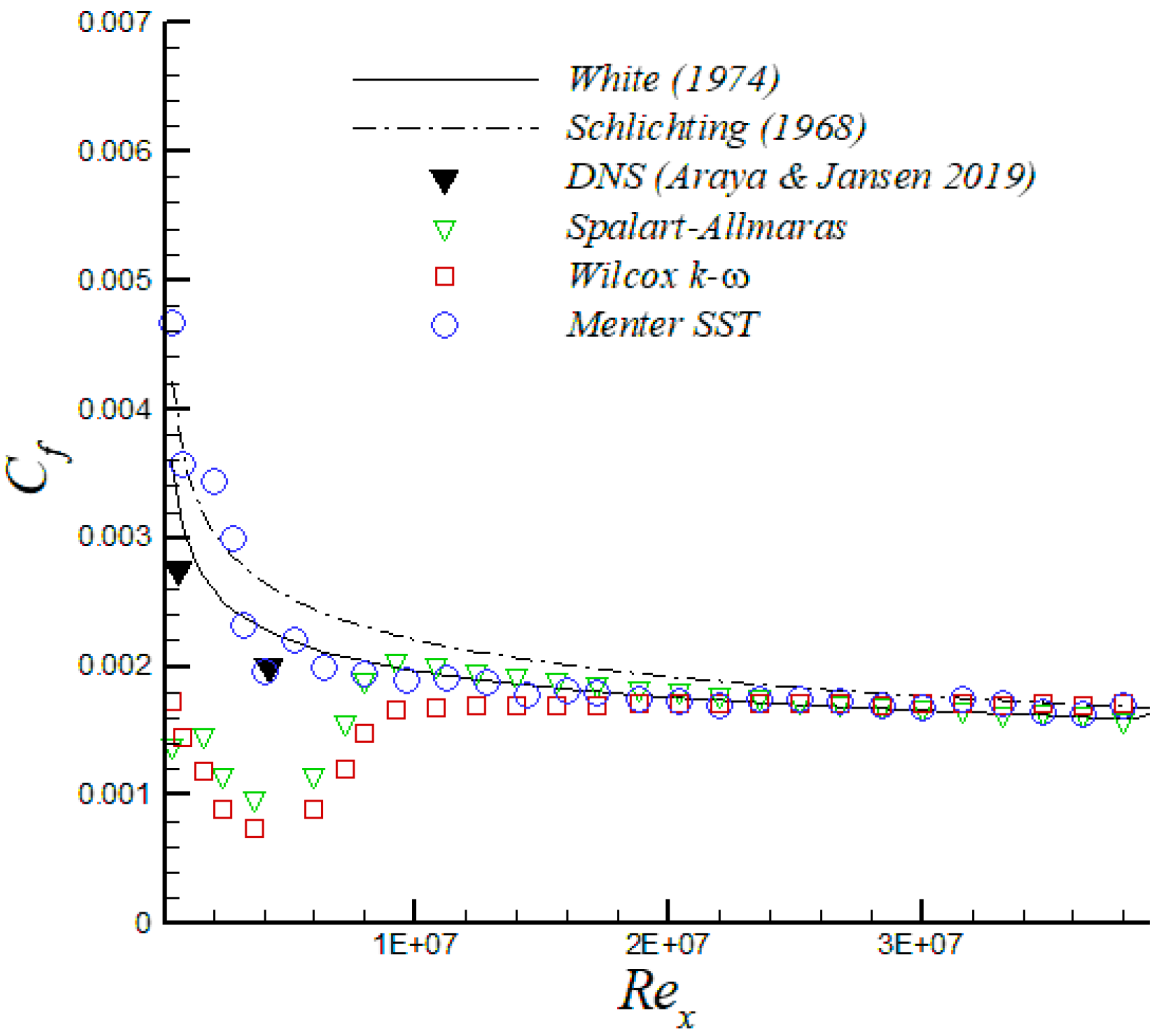
Figure 2 shows the streamwise variation of the skin friction coefficient, , as a function of . Generally speaking, the corresponding values obtained by Spalart–Allmaras, Wilcox k- and Menter SST turbulence models depicted an excellent agreement with theoretical correlations from White [22] and Schlichting [23], particularly by the end of the flat plate. However, the Menter SST model exhibited a shorter transition and the profile quickly tended to realistic fully-turbulent values downstream from the leading edge. Additionally, Direct Numerical Simulation (DNS) data from Araya and Jansen [24] are also included for a supersonic isothermal flat plate ( 2.25) at a freestream Mach number, , of 2.5 and low Reynolds numbers. Again, the Menter SST turbulence model exhibited a good agreement of with high spatial/temporal numerical results. Generally speaking, the mean streamwise velocity along the boundary layer followed the DNS profile of Araya and Jansen [24] and the 1/7 power-law distribution in the outer region (i.e., 0.1), as shown in Figure 3a for . Nevertheless, all velocity profiles computed from turbulence models depicted some deviations in the inner region (where the 1/7 power law did not work properly) from the DNS profile. The thermal boundary layer plays a crucial role in the transport phenomena of compressible wall-bounded flows; consequently, its accurate understanding and modeling are very important. In other words, the coupled behavior of the velocity and thermal field should be properly represented. In Figure 3b, the computed temperature distributions, , as a function of the mean streamwise velocity, , are plotted at a streamwise station where . For comparison, the theoretical Crocco–Busemann relation (see page 502 in White [22]) is also included. The Crocco–Busemann relation assumes a linear variation of the total enthalpy across the boundary layer in zero pressure gradient with a unitary turbulent Prandtl number. Furthermore, present RANS thermal profiles showed good agreement with the quadratic Crocco–Busemann relationship. It is worth mentioning that the Crocco–Busemann relation is a function of the local wall-temperature; therefore, a slightly different theoretical profile was obtained for each turbulence model.
7.2. Transonic RAE 2822 Airfoil
This evaluation test consisted on the simulation of steady turbulent transonic flow around the RAE2822 airfoil, which is the standard test Case 9 [25] for turbulence modeling. The freestream Mach number was , the Reynolds number was and the angle of attack was 2.79°. This problem was solved using a 3D hybrid and unstructured mesh. The mesh consisted of 4.2 million tetrahedral elements, 1.9 million prismatic elements and 2 thousand pyramid elements. The total number of elements was approximately 6.1 million. The boundary layer consisted of 40 layers with the closest point to the wall located at a distance of or approximately 0.1–0.4 in wall units.
Table 1 shows the computed values of lift, drag and moment coefficients for the Spalart–Allmaras, Wilcox k- and Menter SST turbulence models, together with experimental data from the AGARD AR–138 report [25] and other numerical simulations in 2D and structured meshes [26,27]. In Table 1, stands for Not Available. For this simulation case, all turbulence models produced values of within 11 lift counts (1 lift count = 0.001) with respect to experiments by Cook et al. [25]. Similarly, the predicted total drag coefficients, , showed good agreement with experiments with a maximum discrepancy of 1.5 drag counts (1 drag count = 0.0001), at most, for the Menter SST model; nevertheless, it generated the most accurate moment coefficient at 25% of the chord, .
In general, the three models are in good agreement with the experimental results and other simulation values, as shown in Table 1. Furthermore, the pressure () and skin friction () coefficients are depicted in Figure 4, together with the corresponding experimental data from the AGARD AR–138 report [25]. The predicted values of in the upper surface looked very similar in all turbulence models. The weak shock at was not fully captured by turbulence models with discrepancies in the order of 9% in peaks of . Downstream, a quasi-zero pressure gradient zone with almost constant values of and about half-chord in length was observed. The second and stronger shock located at was accurately captured by all models. Perhaps, the Menter SST slightly separated from the experimental values by the end of the shock (i.e., ). The strong shock was characterized by a sharp increase of wall pressure. The presence of a very strong APG induced a small flow separation zone, which is discussed below. Beyond this zone of “pockets” with supersonic flow, the wall pressure kept increasing towards the trailing edge, but at a moderate rate. In addition, the numerical predictions of on the lower surface were almost identical to the experimental values given by all turbulence models. The skin friction coefficient is defined as , where is the wall shear stress, and and are the density and velocity at the edge of the boundary layer, respectively. From the results in Figure 4b, it was inferred that the closest values to experiments were produced by the Menter SST model in the upper side, particularly at the strong shock location (i.e., ). Furthermore, the Spalart–Allmaras and Wilcox k- models were observed to perform similarly; however, the Wilcox k- was the only turbulence model that predicted a shock-induced separation due to the presence of a very strong APG, with a small recirculating zone around 0.55 0.60, as shown in Figure 4b. All models slightly underpredicted the experimental value of the skin friction on the lower surface. Figure 5 shows iso-contours of the Mach number for the Wilcox k- model. This transonic regime was characterized by the formation of regions or “pockets" with supersonic flow. Since the flow must return to its freestream conditions by the time of reaching the trailing edge, this caused the formation of a strong shock by where subsonic flow was observed beyond that point.
During the mesh generation, a good resolution was ensured by clustering the first-off wall point well inside the linear viscous layer (i.e., ) to accurately predict the skin friction coefficient. Accordingly, the distance distribution of the first off-wall point in wall units, , along the RAE2822 airfoil and based on the Menter SST model is shown in Figure 6 together with the airfoil coordinates in the right vertical axis. It can be seen that was around 0.4 in the vicinity of the leading edge for the lower surface; however, was lower than 0.1 in the upper surface, where the flow faced more complex pressure changes. Consequently, the high spatial resolution of the employed mesh was demonstrated. In Figure 7, profiles of the mean streamwise velocity downstream of the strong shock in the upper surface (i.e., at 0.65 and 0.75) are depicted. Notice that the mean streamwise velocity was normalized by the local velocity at the edge of the boundary layer, . In general, for velocity profiles shown in Figure 7a,b, the Menter SST model produced the most accurate velocity profiles of the three turbulence models tested in this study, when compared to experimental values from Cook et al. [25]. It is interesting to point out that both velocity profiles at 0.65 and 0.75 were located in a zone of very strong APG or increasing pressure, as shown in Figure 4a. Furthermore, the Shear Stress Transport (SST) formulation by Menter [19] focused on improving the performance of this turbulence model in adverse pressure gradient flows. Thus, the results depicted in Figure 7a,b support the previous statement. In addition, the corresponding displacement thickness, , momentum thickness, , and, shape factor H () were computed at these stations. These integral boundary layer parameters (i.e., and ) are defined as follows for compressible flows,
where subscripts e stands for values at the edge of the boundary layer. In Table 2, the computed values of , and H are exhibited for the three turbulence models together with experimental data from Cook et al. [25]. Furthermore, it was established that the three models analyzed in this investigation gave a similar level of accuracy on the calculation of the boundary layer parameters; nevertheless, the Menter SST was slightly superior to the other models with an average discrepancy of 5% with respect to experiments. In addition, the knowledge of the shape factor, H, in turbulent flows is important in assessing how strongly the APG is imposed. In fact, the higher is the value of H, the stronger is the APG. Similarly, it is well known that any flow subjected to strong deceleration is prone to separation, where most of the turbulence models find enormous difficulties. In this opportunity, we picked up two stations in the RAE2822 airfoil (i.e., = 0.65 and 0.75) with strong APG or high shape factors. The idea was to evaluate the performance of the turbulence models in extreme conditions. Generally speaking, the Menter SST model showed the best performance in describing the physics of the flow subjected to strong APG.
7.3. ONERA M6 Wing
The third test case considered the simulation of the flow over the ONERA M6 wing [28], where the freestream Mach number was , the angle of attack was and the Reynolds number based on the mean geometric chord was . The hybrid mesh employed consisted of 6.3 million tetrahedral elements, 2.5 million prisms and 11.6 thousand pyramids. The surface mesh consisted of 1.1 million triangular elements. The mesh had 35 viscous layers and the first off-wall point was located at in wall units.
The values of lift and drag coefficient for the Spalart–Allmaras, Wilcox k- and Menter SST turbulence models are shown in Table 3 together with numerical results from Le Moigne and Qin [29] and Nielsen and Anderson [30]. A maximum of nine lift counts deviation in the lift coefficient between the three turbulence models was observed. In addition, a maximum of 14 drag counts difference in the drag coefficient was computed, of which nine drag counts were due to the friction contribution to the drag coefficient. Furthermore, the present numerical results of lift and drag coefficients are in good agreement with numerical values by Le Moigne and Qin [29] and Nielsen and Anderson [30], who employed the Baldwin–Lomax and Spalart–Allmaras turbulence model, respectively. The pressure coefficient profiles at different sections across the wing span are depicted in Figure 8. All three models captured reasonably well the corresponding location of both shocks at each wing span section, given by abrupt modifications on . The most significant discrepancies were observed at , where none of the three models were able to appropriately represent the shock within 0.25 << 0.35. However, a similar behavior of the Spalart–Allmaras and Wilcox k- turbulence models at was reported by Huang et al. [31], Jakirlić et al. [32] and Nielsen and Anderson [30]. The skin friction coefficient is plotted in Figure 9 at spanwise stations = 0.9 and 0.95. These figures show the good agreement among all turbulence models about the location of the flow separation point 0.25 and 0.2 for = 0.9 and 0.95, respectively. The downstream recovery of was different in all turbulence models, with the Wilcox k- and Menter SST turbulence models predicting similar reattachment lengths and Spalart–Allmaras producing the largest reattachment length. The Menter SST model induced higher values for the skin friction downstream of the reattachment point, which was consistent with the largest values of shown in Table 3.
Figure 10 shows iso-surfaces of negative streamwise velocities normalized by the freestream velocity . The recirculating flow bubble in dark blue (identified by a white circle) predicted by the Spalart–Allmaras model was slightly larger than that of predicted by the Menter SST model. Iso-contours of the streamwise velocity, normalized by the freestream velocity , are depicted in Figure 11 in Menter SST at , where a strong shock wave can be clearly observed around 0.25 of the upper surface. Furthermore, the interaction of this shock with the turbulent boundary layer provoked a recirculating zone represented by the dark blue area.
7.4. Generic F15 Aircraft Configuration
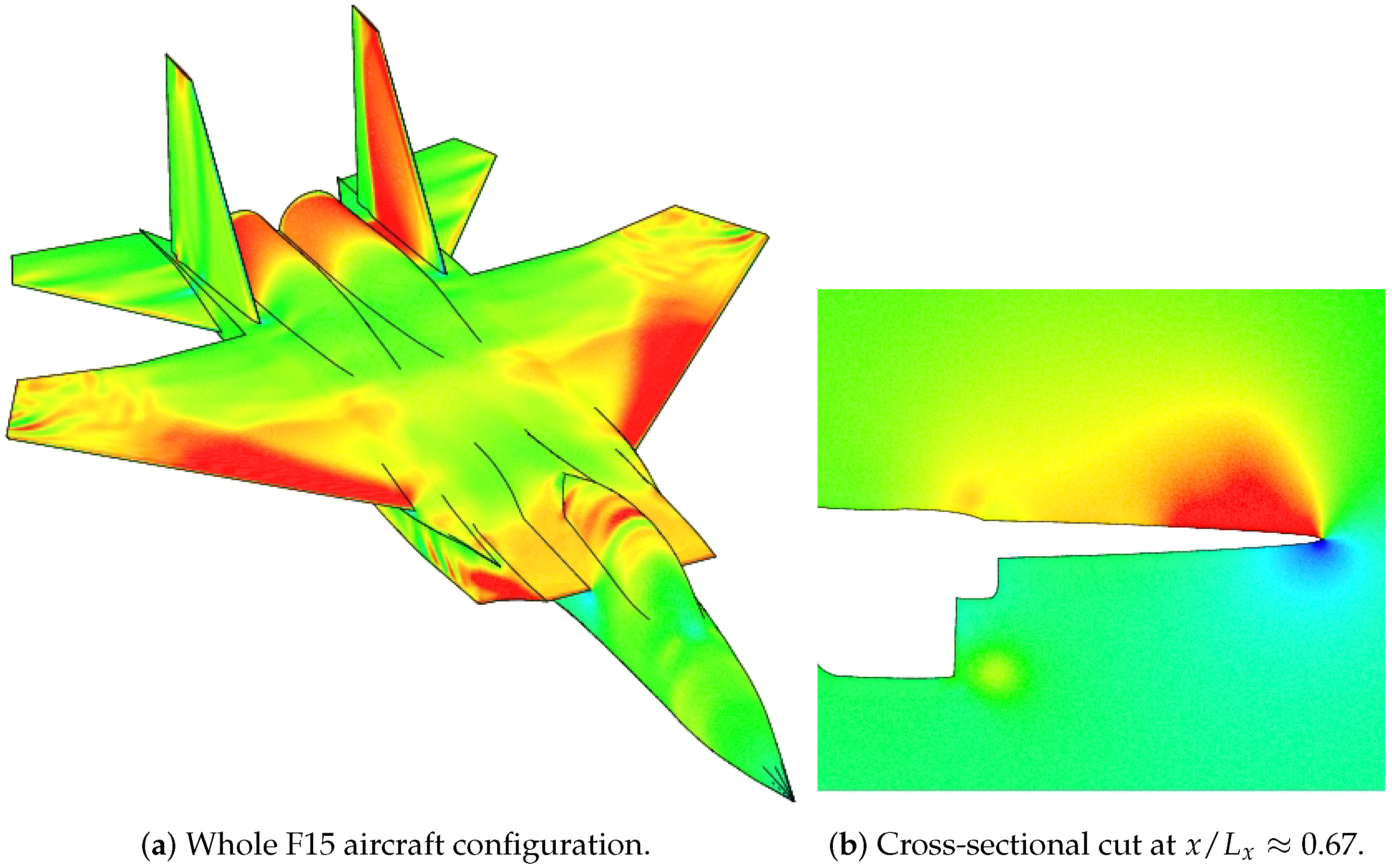
The last example corresponds to a generic F15 aircraft configuration, which represents a very complex and challenging geometry for CFD simulations with concave and convex surface curvatures. The freestream Mach number was , the Reynolds number, based on the airplane length ( 18 m), was and the angle of attack was five degrees. The hybrid mesh consisted of 12.5 million nodes and 49 million elements (36 million tetrahedra, 12.7 million prisms and 48.5 thousand pyramids). Due to the spanwise symmetry nature of the problem, only half of the model was used for the simulation. In Figure 12a, the employed surface mesh is plotted by mirroring the half-aircraft grid across the symmetry plane. In addition, details of the viscous layers can be seen by means of the cut plane at in Figure 12b. Additionally, the boundary layer was made of 44 layers and the first off-wall point was prescribed at m, which ensured that the location of this point was in the linear viscous layer for an accurate skin friction computation. A great deal of thought was given to the design of all computational meshes and dimensions in the present study to ensure grid-independent numerical results. The selected mesh spacing distribution, shown in this section, was the result of grid convergence study that was carried out to obtain grid independent results. The numerical simulations were run on 128 processors. Table 4 shows the lift coefficient, , and the drag coefficient, , for each turbulence model. The numerical results of obtained by the three turbulence models were consistent with a maximum difference of seven lift counts. Furthermore, the largest discrepancy observed in the coefficient was 24 drag counts between the Menter SST and Wilcox k- turbulence models.
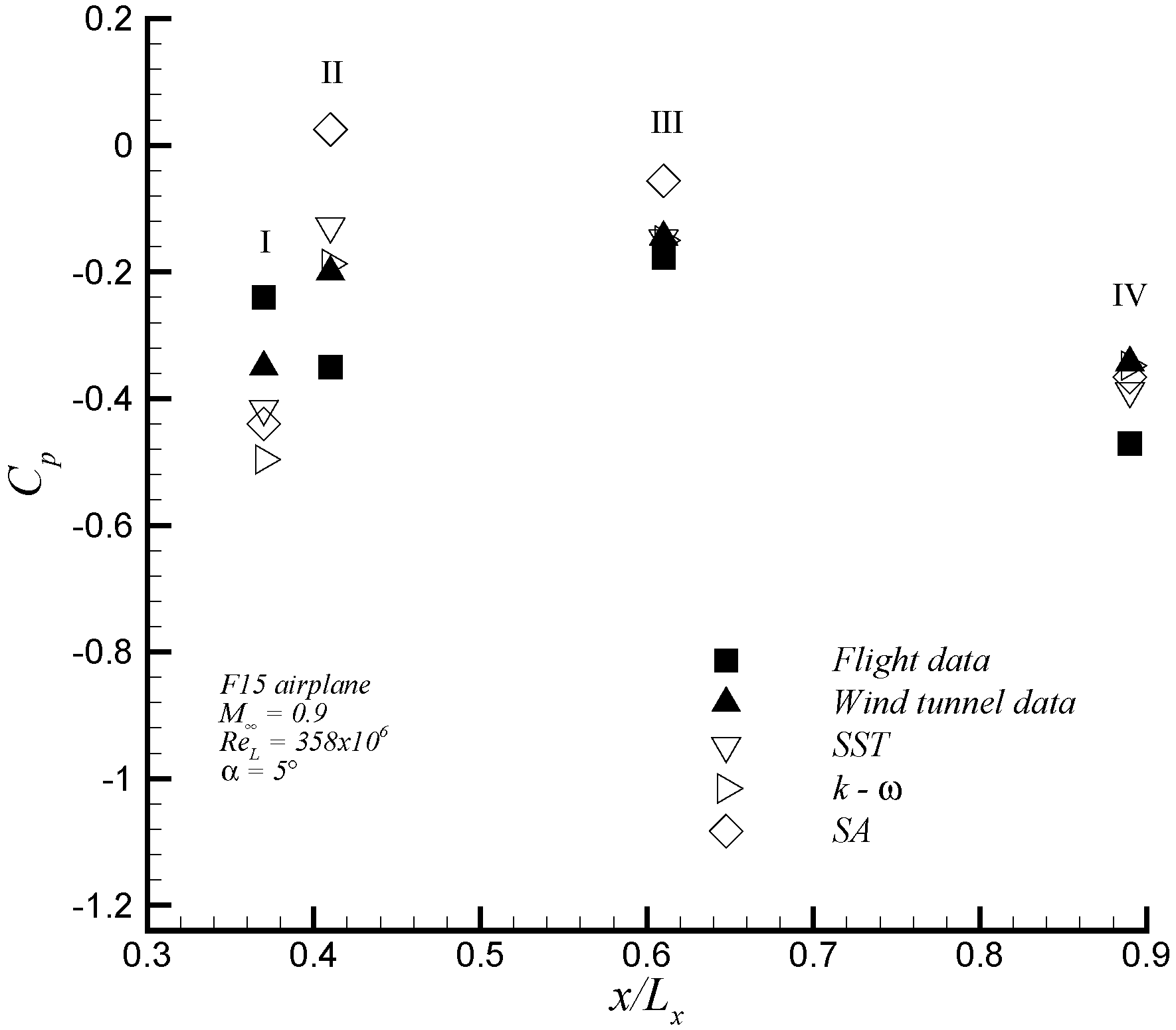
In Figure 13a, iso-contours of the pressure coefficient over the entire F15 aircraft configuration are depicted. Strong shock waves were observed on the canopy over the cock pit, leading edge of wings and between the vertical tails. The cut plane in Figure 13b at depicted high values of toward the wing tip. In addition, a top view of iso-contours of are shown in Figure 14. The value of the pressure coefficient at four points (labeled as I–IV in Figure 14) were compared with flight and wind tunnel data from Webb et al. [33], as shown in Figure 15. In general, the present numerical results are in good agreement with the experimental wind tunnel data. Furthermore, it can be noticed that the pressure coefficients given by the Menter SST model showed a better match with experimental data than those calculated by Spalart–Allmaras and Wilcox k- models. In addition, the most significant discrepancies of the numerical results of with experiments were found in the region , just above the turbine intake. The discrepancy can be attributed to the difference between the estimated engine mass flow prescribed and the used engine mass flow during the flight test. This was emphasized by the significant scattering between the experimental data (in flight and wind tunnel), particularly, at Points I and II. In this zone, the different turbulence models predicted different separation regions, which are discussed below. Hence, this resulted in different local flow patterns that induced different pressure coefficients.
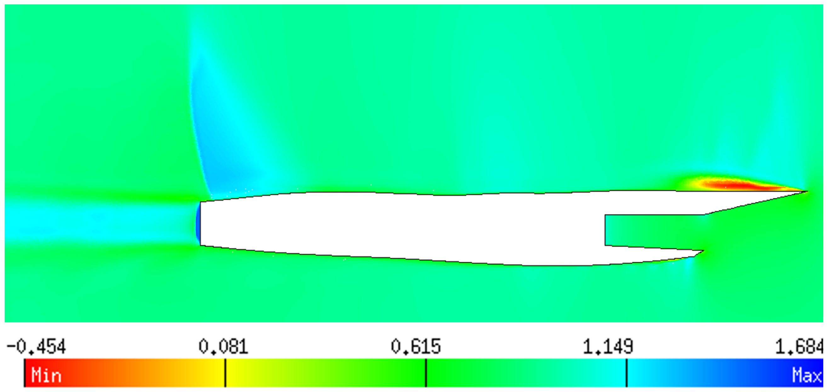
The skin friction coefficient at a spanwise location of or , where m is the semi-span length of the aircraft, is plotted in Figure 16. The study of the drag coefficient due to friction showed that this section had the largest discrepancy between the three turbulence models, as observed in Figure 16a. Figure 16b indicates that the Wilcox k- model predicted two separation bubbles at and 0.36, respectively, while the other two models predicted a single separated region (i.e., at ) with the Menter SST predicting a much larger separation region than that computed by the Spalart–Allmaras model. Furthermore, the iso-contours of streamwise velocity (normalized by the freestream velocity ) by the Menter SST model, as shown in Figure 17, indicated the presence of a lengthy recirculation zone with negative values of the velocity above the turbine intake, given by the shock wave-boundary layer interaction.
Figure 18 and Figure 19 show the pressure coefficients on the upper and lower surfaces of the wing at two different spanwise locations, and 0.59, respectively. In addition, the vertical coordinates, z, of the local profile are represented by the vertical axis on the right. It is shown in Figure 18a that, at , the profiles predicted by the three turbulence models showed similar upper peak values in the vicinity of the leading edge, i.e., . Hence, it can be concluded that the pressure difference between the surface static pressure to the freestream static pressure was equal to the freestream dynamic pressure in absolute value at this location. On the other hand, the Wilcox k- model predicted a stronger second shock wave located at . In the lower side, a moderate APG zone was observed in 0.55 0.6, as shown in Figure 18b, followed by a nearly ZPG region. Furthermore, Figure 19a shows similar peak values of in the upper surface and close to the leading edge at station by all three turbulence models. However, the Spalart–Allmaras model predicted a much stronger second shock located further downstream of the leading edge (at ) than those predicted by the Menter SST and Wilcox k- model. All turbulence models exhibited similar distributions in the lower surface, as shown in Figure 19b.
8. Conclusions
An assessment of three popular turbulent models was performed in 3D aerodynamic cases. The FLITE3D flow solver, in conjugation with the Spalart–Allmaras, the Wilcox k- and the Menter SST turbulence models, was applied to the supersonic flat plate, RAE2822 airfoil, ONERA M6 wing, and F15 aircraft.
The Menter SST model exhibited a short developing section in the supesonic flat plate downstream of the edge. The transonic RAE2822 airfoil possessed a strong shock–boundary layer interaction with an induced separation. The ONERA M6 wing exhibited a very complex flow phenomena such as double shocks, strong APG and streamline curvature effects. In addition, the computed global lift and drag coefficients ( and ) over the F15 aircraft by all turbulence models were very consistent; however, local pressure coefficients by the Menter SST model were in better agreement with experimental values in [33].
Generally speaking, numerical results have been very consistent for the three turbulence models. For attached flows or middle separated flows, there was not a clear superiority of the two-equation turbulence models over the one-equation Spalart–Allmaras model. However, the contrary was observed in separated flows with recirculation zones. Particularly, the Menter SST model showed the best compromise between accurately describing the physics of the flow and numerical stability. The Shear Stress Transport (SST) formulation might be the reason for this. Future investigation will focus on unsteady flow simulations. This could be more appropriate in realistically capturing the complex turbulent structures governed by shock-boundary layer interactions and highly-separated flows; in particular, at the transonic regime.
Funding
This material was based upon work supported by the Air Force Office of Scientific Research (AFOSR) under award number FA9550-17-1-0051.
Acknowledgments
The author acknowledges Oubay Hassan and Kenneth Morgan for valuable insight. Christian Lagares is acknowledged for important discussion.
Conflicts of Interest
The author declare no conflict of interest.
References
- Pope, S.B. Turbulent Flows; Cambridge University Press: Cambridge, UK, August 2000. [Google Scholar]
- Moin, P.; Mahesh, K. Direct Numerical Simulation: A Tool in Turbulence Research. Annu. Rev. Fluid Mech. 1998, 30, 539–578. [Google Scholar] [CrossRef]
- Meneveau, C.; Katz, J. Scale-invariance and turbulence models for large-eddy simulation. Annu. Rev. Fluid Mech. 2000, 32, 1–32. [Google Scholar] [CrossRef]
- Frohlich, J.; von Terzi, D. Hybrid LES/RANS methods for the simulation of turbulent flows. Prog. Aerosp. Sci. 2008, 44, 349–377. [Google Scholar] [CrossRef]
- Catalano, P.; Amato, M. An evaluation of RANS turbulence modelling for aerodynamic applications. Aerosp. Sci. Technol. 2003, 7, 493–509. [Google Scholar] [CrossRef]
- Knight, D.; Yan, H.; Panaras, A.G.; Zheltovodov, A. Advances in CFD prediction of shockwave turbulent boundary layer interactions. Prog. Aerosp. Sci. 2003, 39, 121–184. [Google Scholar] [CrossRef]
- Manzari, M.T.; Hassan, O.; Morgan, K.; Weatherill, N.P. Turbulent flow computations on 3D unstructured grids. Finite Elem. Anal. Des. 1998, 30, 353–363. [Google Scholar] [CrossRef]
- Sørensen, K.A.; Hassan, O.; Morgan, K.; Weatherill, N.P. A multigrid accelerated hybrid unstructured mesh method for 3D compressible turbulent flow. Comput. Mech. 2003, 31, 101–114. [Google Scholar] [CrossRef]
- Peiró, J.; Peraire, J.; Morgan, K. FELISA System Reference Manual. Part 1—Basic Theory; Swansea Report C/R/821/94; University of Wales: Wales, UK, 1994. [Google Scholar]
- Peraire, J.; Morgan, K.; Peiró, J. Unstructured finite element mesh generation and adaptive procedures for CFD. In Applications of Mesh Generation to Complex 3D Configurations; AGARD: Paris, France, 1990. [Google Scholar]
- Hassan, O.; Morgan, K.; Probert, E.J.; Peraire, J. Unstructured tetrahedral mesh generation for three-dimensional viscous flows. Int. J. Numer. Methods Eng. 1996, 39, 549–567. [Google Scholar] [CrossRef]
- Weatherill, N.P.; Hassan, O. Efficient three–dimensional Delaunay triangulation with automatic boundary point creation and imposed boundary constraints. Int. J. Numer. Methods Eng. 1994, 37, 2005–2039. [Google Scholar] [CrossRef]
- Jameson, A.; Schmidt, W.; Turkel, E. Numerical simulation of the Euler equations by finite volume methods using Runge–Kutta timestepping schemes. In Proceedings of the 14th Fluid and Plasma Dynamics Conference, Palo Alto, CA, USA, 13–25 June 1981; AIAA Paper. pp. 81–1259. [Google Scholar]
- Harten, A.; Lax, P.D.; van Leer, B. On upstreaming differencing and Godunov-type schemes for hyperbolic conservation laws. SIAM Rev. 1983, 25, 35. [Google Scholar] [CrossRef]
- Morgan, K.; Peraire, J.; Peiro, J.; Hassan, O. The computation of 3-dimensional flows using unstructured grids. Comput. Methods Appl. Mech. Eng. 1991, 87, 335–352. [Google Scholar] [CrossRef]
- Sørensen, K.A. A Multigrid Accelerated Procedure for the Solution of Compressible Fluid Flows on Unstructured Hybrid Meshes. Ph.D. Thesis, University of Wales, Swansea, Wales, 2002. [Google Scholar]
- Wilcox, D.C. Turbulence Modeling for CFD; DWC Industries, Inc.: La Canada, CA, USA, 2006. [Google Scholar]
- Spalart, P.R.; Allmaras, S.R. A one equation turbulence model for aerodynamics flows. In Proceedings of the 30th Aerospace Science Meeting and Exhibit, Reno, NV, USA, 6–9 January 1992. AIAA Paper 92-0439. [Google Scholar]
- Menter, F.R. Review of the shear-stress transport turbulence model experience from an industrial perspective. Int. J. Comput. Fluid Dyn. 2009, 23, 305–316. [Google Scholar] [CrossRef]
- Geuzaine, P. An Implicit Upwind Finite Volume Method for Compressible Turbulent Flows on Unstructured Meshes. Ph.D. Thesis, Université de Liège, Liège, Belgium, 1999. [Google Scholar]
- Spalart, P.R.; Rumsey, C.L. Effective Inflow Conditions for Turbulence Models in Aerodynamic Calculations. AIAA J. 2007, 45, 2544–2553. [Google Scholar] [CrossRef] [Green Version]
- White, F.M. Viscous Fluid Flow; McGraw Hill: New York, NY, USA, 1974. [Google Scholar]
- Schlichting, H. Boundary Layer Theory; McGraw Hill: New York, NY, USA, 1968. [Google Scholar]
- Araya, G.; Jansen, K. Compressibility effect on spatially-developing turbulent boundary layers via DNS. In Proceedings of the 4th Thermal and Fluids Engineering Conference (TFEC2019), Las Vegas, NV, USA, 14–17 April 2019. [Google Scholar]
- Cook, P.; McDonald, M.; Firmin, M. Aerofoil RAE2822 Pressure Distributions and Boundary Layer and Wake Measurements; Report AR-138; AGARD: Paris, France, 1979. [Google Scholar]
- Hirschel, E.H. Finite Approximations in Fluid Mechanics II: DFG Priority Research Program, Results 1986–1988; Notes on Numerical Fluid Mechanics; Vieweg: Braunschweig, Germany; Wiesbaden, Germany, 1989; Volume 25. [Google Scholar]
- Swanson, R.C.; Rossow, C.C. An efficient solver for the RANS equations and a one-equation turbulence model. Comput. Fluids 2011, 42, 13–25. [Google Scholar] [CrossRef]
- Schmitt, V.; Charpin, F. Pressure Distributions of the ONERA M6 Wing at Transonic Mach Numbers; Report AR-138; AGARD: Paris, France, 1979. [Google Scholar]
- LeMoigne, A.; Qin, N. Variable-fidelity aerodynamic optimization for turbulent flows using a discrete adjoint formulation. AIAA J. 2004, 42, 1281–1192. [Google Scholar]
- Nielsen, E.J.; Anderson, W.K. Recent improvements in aerodynamic sesign optimization on unstructured meshes. AIAA J. 2002, 40, 1155–1163. [Google Scholar] [CrossRef]
- Huang, J.C.; Lin, H.; Yang, J.Y. Implicit preconditioned WENO scheme for steady viscous flow computation. J. Comput. Phys. 2009, 228, 420–438. [Google Scholar] [CrossRef]
- Jakirlić, S.; Eisfeld, B.; Jester-Zurker, R.; Kroll, N. Near-wall, Reynolds-stress model calculations of transonic flow configurations relevant to aircraft aerodynamics. Int. J. Heat Fluid Flow 2007, 28, 602–615. [Google Scholar] [CrossRef]
- Webb, L.; Varda, D.; Whitmore, S. Flight and Wind-Tunnel Comparisons of the Inlet/Airframe Interaction of the F-15 Airplane; Technical Paper 2374; NASA: Washington, DC, USA, 1984.
Figure 1.
Mesh schematic (a); close-up of the near wall region (b); and iso-contours of turbulent kinetic energy from Menter SST (c) in the supersonic flat plate.
Figure 1.
Mesh schematic (a); close-up of the near wall region (b); and iso-contours of turbulent kinetic energy from Menter SST (c) in the supersonic flat plate.

Figure 2.
Skin friction coefficient as a function of .

Figure 3.
Mean streamwise velocity (a); and temperature distribution (b) in the supersonic flat plate.
Figure 3.
Mean streamwise velocity (a); and temperature distribution (b) in the supersonic flat plate.

Figure 4.
Pressure (a); and skin friction (b) coefficient in the RAE2822 airfoil.

Figure 5.
Iso-contours of Mach number (Wilcox k- model).

Figure 6.
Distance distribution of the first off-wall point in wall units along the RAE airfoil for the Menter SST model.
Figure 6.
Distance distribution of the first off-wall point in wall units along the RAE airfoil for the Menter SST model.

Figure 7.
Mean streamwise velocity distribution in the RAE2822 airfoil.

Figure 8.
Pressure coefficient distributions in the ONERA M6 wing at .


Figure 9.
Skin friction distribution in the ONERA M6 wing at

Figure 10.
Iso-surfaces of streamwise velocity over the upper surface in the ONERA M6 wing at (flow from left to right).
Figure 10.
Iso-surfaces of streamwise velocity over the upper surface in the ONERA M6 wing at (flow from left to right).

Figure 11.
Iso-contours of streamwise velocity in Menter SST at (a) and zoom over the leading edge (b) in the ONERA M6 wing at (flow from right to left).
Figure 11.
Iso-contours of streamwise velocity in Menter SST at (a) and zoom over the leading edge (b) in the ONERA M6 wing at (flow from right to left).

Figure 12.
Surface mesh in the F15 aircraft configuration.

Figure 13.
Iso-contours of the pressure coefficient in the F15 aircraft configuration (Cp range of color contour as in Figure 14).
Figure 13.
Iso-contours of the pressure coefficient in the F15 aircraft configuration (Cp range of color contour as in Figure 14).

Figure 14.
Iso-contours of pressure coefficient in the upper surface of the F15 aircraft.

Figure 15.
Variation of the pressure coefficient in the top surface along of F15 aircraft for present numerical data (open symbols) experimental data (closed symbols).
Figure 15.
Variation of the pressure coefficient in the top surface along of F15 aircraft for present numerical data (open symbols) experimental data (closed symbols).

Figure 16.
Skin friction coefficient in the upper surface of F15 at (a); and zoom of the separated flow zone (b).
Figure 16.
Skin friction coefficient in the upper surface of F15 at (a); and zoom of the separated flow zone (b).

Figure 17.
Iso-contours of the streamwise velocity at (flow from right to left).

Figure 18.
Pressure coefficients of F15 in the upper (a) and lower (b) surfaces at .

Figure 19.
Pressure coefficients of F15 in the upper (a) and lower (b) surfaces at .


Table 2.
Boundary layer parameters at = 0.65 and 0.75 in the RAE2822 airfoil.
| Location | Parameter | SA | k- | SST | Exp. [25] |
|---|---|---|---|---|---|
| H | |||||
| H |
Table 3.
Lift and drag coefficients in ONERA M6 wing at .
| Aerodynamic Coeff. | SA | k- | SST | Num. [29] | Num. [30] |
|---|---|---|---|---|---|
| N/A |
Table 4.
Lift and drag coefficients in F15 aircraft at .
| Aerodynamic Coeff. | Spalart–Allmaras | Wilcox k- | Menter SST |
|---|---|---|---|
© 2019 by the author. Licensee MDPI, Basel, Switzerland. This article is an open access article distributed under the terms and conditions of the Creative Commons Attribution (CC BY) license (http://creativecommons.org/licenses/by/4.0/).
Share and Cite
MDPI and ACS Style
Araya, G. Turbulence Model Assessment in Compressible Flows around Complex Geometries with Unstructured Grids. Fluids 2019, 4, 81. https://doi.org/10.3390/fluids4020081
AMA Style
Araya G. Turbulence Model Assessment in Compressible Flows around Complex Geometries with Unstructured Grids. Fluids. 2019; 4(2):81. https://doi.org/10.3390/fluids4020081
Chicago/Turabian StyleAraya, Guillermo. 2019. "Turbulence Model Assessment in Compressible Flows around Complex Geometries with Unstructured Grids" Fluids 4, no. 2: 81. https://doi.org/10.3390/fluids4020081