Ionic Fracture Fluid Leak-Off

1
Lavrentyev Institute of Hydrodynamics, Novosibirsk State University, Novosibirsk 630090, Russia
2
Trofimuk Institute of Oil and Gas Geology and Geophysics, Novosibirsk State University, Novosibirsk 630090, Russia
*
Author to whom correspondence should be addressed.
Fluids 2019, 4(1), 32; https://doi.org/10.3390/fluids4010032
Submission received: 10 January 2019
/
Revised: 5 February 2019
/
Accepted: 15 February 2019
/
Published: 19 February 2019
(This article belongs to the Special Issue Electro- and Magneto-hydrodynamic Manipulation of Particles Suspended in Fluids)
Abstract
:The study is motivated by monitoring the space orientation of a hydrolic fracture used in oil production. Streaming potential arises due to the leakage of ionic fracking fluid under the rock elastic forces which make the fracture disclosure disappear after pumping stops. The vector of electric field correlates with the fracture space orientation since the fluid leakage is directed normally to the fracture surfaces. We develop a mathematical model for the numerical evaluation of the streaming potential magnitude. To this end, we perform an asymptotic analysis taking advantage of scale separation between the fracture disclosure and its length. The contrast between the virgin rock fluid and the fluid invading from the fracture is proved to be crucial in a build up of a net charge at the invasion front. Calculations reveal that an increase of the viscosity and resistivity contrast parameters results in an increase of the streaming potential magnitude. Such a conclusion agrees with laboratory experiments.
1. Introduction
In applying hydraulic fracturing treatment of rocks, one should prepare for execting the size of a fracture and its space orientation. One of the reasons is to avoid hydraulic connectivity of a production well with an injection one, since during water-flood of an initially oil-filled reservoir, encroaching water spoils hydrocarbon recovery. Directional fracturing is also of importance in petrothermal power production while designing geothermal circulation systems within the dry rocks [1]. Typical circulation systems consist of two wells connected by a fracture. By injecting water into the hot, deep, crystalline rocks, a huge amount of heat can be harnessed [2].
The pressure transient data during the injection fall-off test provide a way to determine the dimensions of an induced fracture but not its direction [3]. Microseismic measurements allow us to find the direction of the fracture [4]. However, the reliability of such measurements is not evident due to the extremely low energy of microseismic events and a high level of acoustic noise. Therefore, alternative approaches are of interest.
In this study, we estimate the electric field induced near the hydrofracture by leakage of a contrast fluid from the fracture under elastic forces in the rock which make the fracture disclosure disappear after pumping stops. The electric potential, known as the streaming potential, arises due to electrokinetic phenomena when ionic fluid moves through a porous rock [5]. The vector of the induced electric field is directed normally to the fracture surfaces, while the electric potential at the fracture surfaces strongly depends on the location of the invasion front of the fracture fluid. Polarization occurs due to charge concentration at the invasion front. The charge density can be evaluated via the resistivity jump across the front.
Streaming potential measurement is based on response (DC voltage) associated with the excess of electrical charge that is transported by flow of conductive fluids through porous media under a pressure gradient or an electrical conductivity change. Such a method presents a key electrokinetic mechanism to study fluid flows in porous media. An electrical double layer (EDL) forms at the rock–fluid interfaces. The onset of fluid flow perturbs the distribution of the ions present in that layer and induces a current, which is the source of the streaming potential. This electrokinetic mechanism has been tested and employed in the laboratory to monitor the evolution of an oil–water encroachment front over time during hydrocarbon recovery Earlier, the streaming potential dynamics were studied near the production well during water-flood of an initially oil-filled [6,7]. Calculations reveal [8] that encroaching water causes changes in the streaming potential at the production well which could be resolved above background electrical noise; water approaching the well could be detected at several 10s to 100s of meters away. The magnitude of the measured potential depends upon the production rate, the coupling between fluid and streaming potentials, and the nature of the front between the displaced oil and the displacing water. Similar results were obtained via simulation for the streaming potential near the injection borehole during drilling [9].
The fact that the induced electric field is orthogonal to the fracture surfaces allows one to tell the fracture direction starting from the electric field testing. If such a field can be strong enough, one can pass to the next step trying to invent a method of measuring the electric field close to the fracture. In this study, we do not address measurements.
In our mathematical approach, we take advantage of the scale difference between fracture disclosure and its length. With fracture disclosure being small, one can reduce fracture–rock interaction onto the central plane between the fracture surfaces. To evaluate the electric field near the fracture, we apply an asymptotic technique assuming that the contrast between the invasion zone and the virgin rock is small. Agreement with laboratory experiments on correlations between the variations of the streaming potential and fluid flow in the core-sample is provided [10]; it follows from our calculations that electric field in the core-sample can be increased in two ways: when the viscosity of the invading fluid decreases or when the electric conductivity of the invading fluid decreases. Thus, the proposed mathematical model explains the laboratory experiments [10] and set theoretical tools for the streaming potential method applied both in the tracking the water front during production operations and the hydro-fracture development.
2. Basic Equations
We treat the fluid-saturated rock as a Bio’s poroelastic medium enjoying quasi-static deformations and incompressible flows which are explained within mathematical models developed in [3,11]. According to this model, the fluid mass balance and the momentum law of the poroelastic medium are given by the equations
Here,
where is the porosity, is the Darcy velocity, is the fluid density, is the solid density, is the effective stress tensor, p is the pore pressure, is the deformation tensor, is the rock displacement vector, is the Biot number, is the gravitational acceleration vector, and are the elasticity moduli. We use the notations
An equilibrium state before fracturing is described by the equations
Here, is the identity tensor, is the equilibrium stress tensor in the rock before fracturing, is the equilibrium pore pressure, is the equilibrium rock displacement. The equilibrium state is determined by regional stresses as follows. Let us consider a vertical cylinder of the thickness which is in equilibrium state and which is compressed from above by a poroelastic medium of thickness h, . It is proved in [3] that vertical load is transmitted to horizontal compression by the formula
where
is the unit external normal vector at the lateral cylinder surface, the point stands for the scalar product, is the Poisson coefficient, is the lateral stress coefficient.
Generally, porosity depends on pore pressure and rock compressibility, i.e., , . By definition of the Biot number , we have the equality [12].
Let us introduce the compressibility coefficient and the deviation quantities
The fluid flux obeys the generalized Darcy law which governs electrolyte flows in a porous medium [13,14,15]:
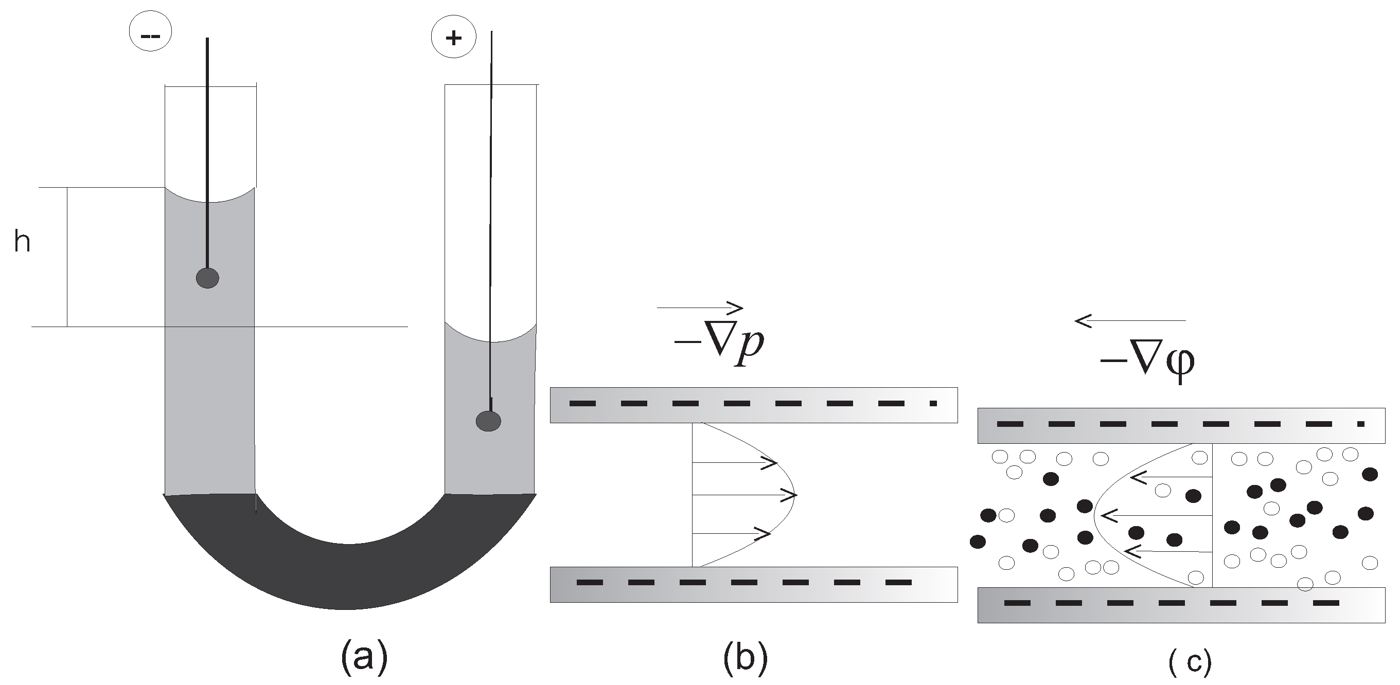
where is the density of electric current, is the streaming potential, are electro-kinetic coefficients. It is the double electric layer (DEL) theory which lays behind the first two equations in (4). Particularly, these equations explain the electro-osmosis effect discovered by F.F. Reuss in 1808, Figure 1. The latter equation in (4) is known as the charge conservation law. By the two-scale homogenization theory, it is proved in [16] that are given by the following representation formulas:
where is the rock permeability, is the dynamical viscosity of the pore fluid, is the effective density of the electric conductivity, F is the dimensionless tortuosity. For sandstones, [8,16].
In [17,18], a mathematical model and a computer code are developed for calculation of the electric conductivity of a saturated rock. The model allows one to determine an optimal Archie-like law
where is the density of the pore fluid electric conductivity, m is the cementation factor, water saturation, q mineralization factor, and is the percolation limit.
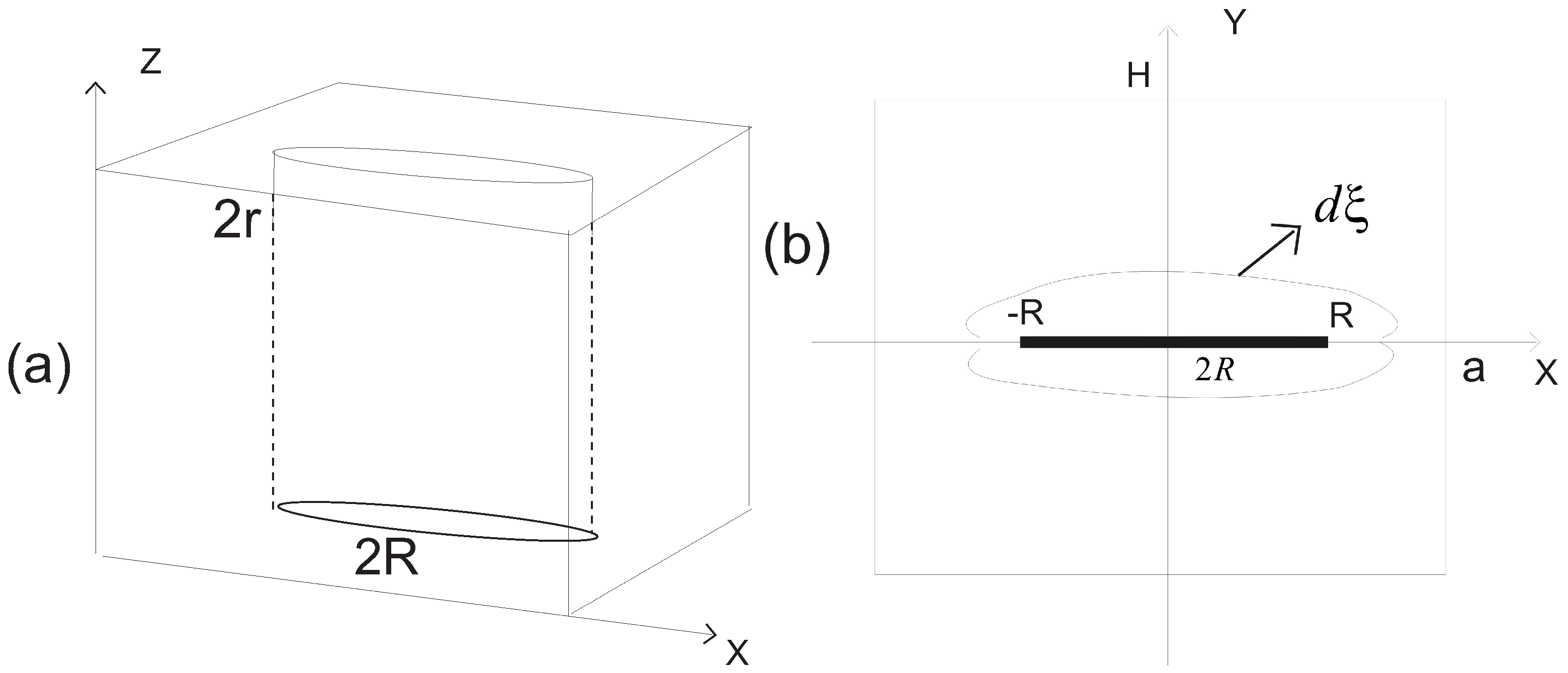
We assume that a vertical fracture of height and length is extended along the horizontal x-axis and its disclosure along another horizontal y-axis does not depend on the vertical variable z, Figure 2a. We also assume that the fracture is symmetrical with respect to the y-axis, and the rock stress-strain state is symmetrical with respect to the x-axis and y-axis. Thus, in what follows we study a two-dimensional problem with all the vectors lying in the horizontal plane .
Let us write the mass conservation law for fracture fluid. As in the lubrication theory, we have (Batchelor, 1967)
Here, w stands for one-half the fracture aperture. By continuity of displacements,
where is the unite vector along the y-axis, q is the fluid leakage, is the fluid velocity along the x-axis. The velocity V enjoys the representation
where is the viscosity of the fracture fluid. It is remarked in [3] that one can use the following alternative formula:
where is the fracture permeability and is the fracture porosity.
Leakage from the fracture satisfies the continuity condition
It was proved in [19,20] that the invasion front can be determined by the method of characteristics from the following equation for the position vector at the -plane:
It means that the infinitesimal displacement of the front point is equal to , Figure 2b.
Let us comment on the front since it plays a crucial role in the study. Mathematically, the front can be associated with the interface , with being a scalar function. It means that the solution of (9) satisfies the equation . Propagation of the interface F along the normal vector can be determined from Equation (9) as follows:
Let us denote by the jump of the function across the interface F along the normal vector at the point :
By continuity,
On the other hand, . Hence, . The latter condition implies that there is a charge concentration at the interface F. In short, our goal is to determine dynamics of the jump .
Let us formulate boundary-value conditions for the fracture lying in the rectangular
Since the fracture aperture is small compared to its length we reduce fracture-rock interactions to its footprint, Figure 1b,
Because of symmetry we study flows and deformations in the half domain only.
We assume that the pressure and stress at the external boundary coincide with the regional values. This is why in terms of deviated quantities we impose the following conditions:
where is the unite vector tangential to the boundary , is the prescribed streaming potential. Stress continuity at the rock–fracture interface reduces to the footprint as follows
where is the streaming potential inside the fracture. Pressure continuity at the rock–fracture interface implies that the pore pressure and the fracture pressure coincide at . Outside the fracture, we impose the following symmetry conditions
To complete the picture, one should set initial conditions. We shall do it in what follows.
3. Very Long Fracture
Our goal is determine correlations between streaming potential dynamics and invasion front propagation. To perform asymptotic analysis, we pass to a simplified problem under the following hypotheses. We assume that the fracture aperture is the same along the fracture, with the latter being infinite. In this case and the solution depends on time and the space variable y only, .
We denote
Omitting the prime in the pressure notation , we arrive at the following equations for the functions in the domain :
Boundary conditions become
It is crucial in the present study that the kinetic coefficients undergo jumps at the invasion front:
with and being different constants.
Let us analyse system (12)–(17). Equation (12) implies that the function does not depend on the variable y. Now, it follows from the boundary condition (17) that . Hence, one can exclude the function v by the formula
One can derive from (17) the following boundary condition for pressure at :
By excluding , we find the following representation for :
where
Here and in what follows, stands for jump of the function at the point :
Thus, by eliminating displacement and potential, we reduce the problem (12)–(17) to the following mathematical model. We look for unknown functions , , satisfying the equations:
Observe, that solution should obey the no-jump restrictions:
Let us pass to dimensionless variables
Now, the functions , satisfy the equations
on the dimensionless interval . Here, are dimensionless parameters:
The kinetic coefficients are stepwise functions:
We denote
The function is given by the formula
By definition, is dimensionless electric current density since and is dimension electric current density.
We formulate initial conditions as follows:
Choosing , we obtain that and . Observe that we study electric field induced by the fracture closing. Hence, initial fracture aperture is assumed known and it will appear in what follows.
The solution obeys the following no-jump restrictions:
Given the functions and , one can determine dimensionless electric field by the formula
4. Asymptotic Analysis
Observe, that (27) is not a differential equation in the common sense since it contains not only partial derivatives of at the running point but at the point also, with being unknown function. It is the main mathematical difficulty of the study. Up to now, no tools are developed to solve the problem numerically. This is why we try to solve it analitically applying an asymptotic analysis. There are publications on differential equations which contain partial derivatives at the running point and a point , with being fixed. Such equations are known as loaded differential equations.
We analyse system (27)–(29) under the assumption that jumps of the coefficients are small in the sense that there is a small such that where the step-wise functions do not depend on . We perform an asymptotic analysis assuming that . Clearly, both the functions and depend on . But there is a difficulty in addressing the difference starting from Equation (27) for . The problem is that the coefficients depend on also and undergo jumps across the moving unknown line . To emphasize that the functions depend on , we write instead of .
The way to avoid this difficulty is to pass to new variables such that all the coefficients are defined on the same fixed domain. We define the change of variables as follows:
In new variables, the function is defined on the fixed interval and the functions , satisfy the equations
where
The functions are defined in Appendix A.
The no-jump conditions at become
We look for , via the expansion series
We prove in Appendix A, that the function in the dimensionless physical variables is given by the formula
Clearly, increases in time even if .
Let us determine approximate dimensionless electric current , making use the formulas
We find that
In dimension variables the density of the electric current is given by the formula [Vms].
Starting from the definition (31), we calculate dimensionless gradient of potential using the formula
Let us introduce the contrast parameters
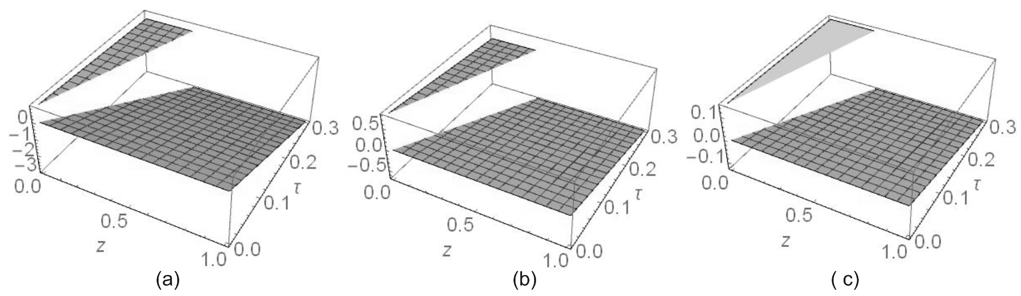
We calculated dynamics of neglecting the second term in (35) which decreases exponentially in time. Figure 3 depicts the reduced potential gradient across the invasion front for the case and different values of b. Potential gradient jump implies charge concentration at the invasion front . The charge concentration is build up as b grows. Observe that the signs of are different before and after the front.
Let us calculate within the fracture assuming that . We have
Due to the formula, , we derive that
Let us estimate magnitude of for the typical values of data given in Nomenclature setting for simplicity. In this case, . Thus, the dimension initial value of the electric field within the fracture is equal to
5. Attenuation Time
The induced electric field exists until the fracture aperture disappears. To estimate the closure time, we introduce one more dimensionless parameter , where L is the one-half the initial fracture aperture. Let stand for dimensionless fracture aperture at the dimensionless moment . Due to (22), can be determined from the equation
We remind that is the dimension initial fracture disclosure. A closure time satisfies the equality
Hence, approximately
With the initial data given by (A2), the above equation is equivalent to
Assuming that and using the formula , we derive that
The dimension closure time is equal to
Setting and applying the typical conditions given in Nomenclature, we find that the dimension closure time is equal to [h], provided [sm]. One more conclusion is that the closure time decreases as the viscosity of fracture fluid decreases also.
6. Discussions and Conclusions
We formulated a mathematical model to evaluate the streaming potential induced by ionic fracture fluid leak-off after shut-in of a water injection well. Such a potential appears due to electro-kinetic effects relevant to electrolyte flows in a porous medium. The contrast between the virgin fluid and the fluid invading from the fracture is proved to be crucial in a build up of net charge at the invasion front. Calculations reveal that increase of the viscosity and resistivity contrasts results in increase of the streaming potential magnitude. To derive basic equations, we used the scale separation between the fracture disclosure and length. We developed an asymptotic series approach starting from the assumption the contrast parameters is small. The study is motivated by the observation that the vector of electric field correlates with the fracture space orientation since it is directed normally to the fracture surfaces.
Author Contributions
Conceptualization, V.S. and M.E.; methodology, V.S. and M.E.; software, V.S.; validation, V.S. and M.E.; formal analysis, V.S.; investigation, V.S. and M.E.; resources, M.E.; data curation, M.E; visualization, V.S.; supervision, M.E.; funding acquisition, M.E.
Funding
The research is partially supported by Grant of Government of Russian Federation No 14.W03.31.0002.
Conflicts of Interest
The authors declare no conflict of interest.
Abbreviations
The following notations are used in this manuscript:
| Biot’s number, dimensionless, | |
| shear elasticity modulus, 8.95 [GPa], 1 [GPa] | |
| bulk elasticity modulus, , [GPa] | |
| Poisson ratio, dimensionless, | |
| fluid density, | |
| solid density, | |
| porosity, dimensionless, 0.2 | |
| total density, | |
| g | gravitational acceleration, |
| S | compressibility, 0.0687 [GPa] |
| H | domain’s size of the nearby zone, 10 [m] |
| L | one-half the initial fracture aperture, 0.5 [cm] |
| T | characteristic time, 3600 [s] |
| reference value of streaming potential, 0.1 [mV], | |
| h | depth, 2500 [m] |
| rock’s weight, | |
| lateral stress coefficient, dimensionless | |
| regional stress, | |
| reference pressure, | |
| rock permeability, , | |
| dynamic viscosity of invasion fluid, 0.33 [cp], 1 [cp] | |
| dynamic viscosity of pore fluid, 3 [cp] | |
| specific electric conductivity of invasion fluid, , | |
| specific electric conductivity of pore fluid, | |
| water saturation, dimensionless, , | |
| m | cementation factor, dimensionless, , |
| percolation porosity limit, dimensionless, | |
| effective electric conductivity of saturated rock, , | |
| F | tortuosity, dimensionless, |
| electrokinetic coefficients | |
| electrokinetic coefficients in invasion zone | |
| electrokinetic coefficients in virgin zone | |
| , dimensionless | |
| , dimensionless | |
| , dimensionless | |
| , dimensionless | |
| , dimensionless | |
| , dimensionless | |
| , dimensionless |
Appendix A
It follows from (32) that
Let us introduce the functions
and denote . Observe that the parameter and the functions , , depend on .
Let us write expansion series for :
Starting from the definition of the functions , we find that , , and
Similarly, we find that
where
Writing the expansion series
one can derive that
Setting the expansion series for , and in Equations (27) and (28), we find that the functions , can be determine from the equations
where
Similarly, we find that the functions and can be determine from the equations
where and
Let us return to the physical dimensionless variables , substituting in (32) by . In the variables , the functions and satisfy the equations
References
- Ziagos, J.; Phillips, B.R.; Boyd, L.; Jelacic, A.; Stillman, G.; Hass, E. Technology roadmap for strategic development of enhanced geothermal systems. In Proceedings of the 38-th Workshop on Geothermal Reservoir Engineering, Stanford, CA, USA, 11–13 February 2013. SGP-TR-198. [Google Scholar]
- Hunsbedt, A.; Kruger, P.; London, A.L. Energy Extraction from a Laboratory Model Fractured Geothermal Reservoir. J. Petrol. Technol. 1978, 30, 712–718. [Google Scholar] [CrossRef]
- Shelukhin, V.V.; Baikov, V.A.; Golovin, S.V.; Davletbaev, A.Y.; Starovoitov, V.N. Fractured water injection wells: Pressure transient analysis. Int. J. Solids Struct. 2014, 51, 2116–2122. [Google Scholar] [CrossRef]
- Le Calvez, J.; Malpini, R.; Xu, J.; Stokes, J.; Williams, M. Hydrolic fracturing insights from microseismic monitoring. Oilfeld Rev. 2016, 28, 16–33. [Google Scholar]
- Ishio, T.; Mizutani, H. Experimental and the theoretical basis of electrokinetic phenomena in rock-water systems and its application in gheophysics. J. Geophys. Res. 1981, 86, 1763–1775. [Google Scholar] [CrossRef]
- Jaafar, M.Z.; Jackson, M.D.; Saunders, J.H.; Vinogradov, J.; Pain, C.C. Measurements of Streaming Potential for Downhole Monitoring on Intelligent Wells; SPE-120460-MS; Society of Petroleum Engineers: Houston, TX, USA, 2009. [Google Scholar]
- Jackson, M.D.; Vinogradov, J.; Saunders, J.H.; Jaafar, M.Z. Laboratory measurements and numerical modeling of streaming potential for downhole monitoring in intelligent wells. SPE J. 2011, 16, 625–636. [Google Scholar] [CrossRef]
- Saunders, J.H.; Jackson, M.D.; Pain, C.C. A new numerical model of electrokinetic potential response during hydrocarbon recovery. Geophys. Res. Lett. 2006, 33, 1–6. [Google Scholar] [CrossRef]
- Eltsov, I.N.; Shelukhin, V.V.; Epov, M.I. Evolution of self-potential near the hole during drilling. Dokl. Earth Sci. 2011, 436, 241–245. [Google Scholar] [CrossRef]
- Ghommem, M.; Qiu, X.; Aidagulov, G.; Abbad, M. Streaming potential measurements for downhole monitoring of reservoir fluid flows: A laboratory study. J. Petrol. Sci. 2018, 161, 28–49. [Google Scholar] [CrossRef]
- Shelukhin, V.V.; Eltsov, I.N. Geodynamics of the zone close to a borehole during drilling. Dokl. Earth Sci. 2012, 443, 537–542. [Google Scholar] [CrossRef]
- Biot, M.A. Theory of elasticity and consolidation for a porous anisotropic solid. J. Appl. Phys. 1955, 26, 182–185. [Google Scholar] [CrossRef]
- Amirat, Y.; Shelukhin, V.V. Homogenization of electroosmotic flow equations in porous media. J. Math. Anal. Appl. 2008, 342, 1227–1245. [Google Scholar] [CrossRef]
- Hartsen, M.W.; Pride, S.R. Electroseismic waves from point sources in layered media. J. Geophys. Res. 1997, 102, 24745–24769. [Google Scholar] [CrossRef]
- Wurmstich, B.; Morgan, F.D. Modeling of streaming potential responses caused by oil pumping. Geophysics 1994, 59, 46–56. [Google Scholar] [CrossRef]
- Shelukhin, V.; Eltsov, I.; Paranichev, I. The electrokinetic cross-coupling coefficient: Homogenization approach. World J. Mech. 2011, 1, 127–136. [Google Scholar] [CrossRef]
- Shelukhin, V.V.; Terentev, S.A. Frequency dispersion of dielectric permittivity and electric conductivity of rocks via two-scale homogenization of the Maxwell equations. Prog. Electromagn. Res. B 2009, 14, 175–202. [Google Scholar] [CrossRef]
- Shelukhin, V.V.; Terentev, S.A. Homogenization of Maxwell equations and the Maxwell-Wagner dispersion. Dokl. Earth Sci. 2009, 424, 155–159. [Google Scholar] [CrossRef]
- Shelukhin, V.V. Invasion around a horizontal wellbore. Eur. J. Appl. Math. 2008, 19, 41–60. [Google Scholar] [CrossRef]
- Shelukhin, V.V.; Eltsov, I.N. Dynamics of near borehole zone while drilling poroelastic layer. Geophys. J. 2012, 34, 265–272. [Google Scholar]
Figure 1.
(a) F.F. Reuss experiment (1808) with water in the U-tube plugged with sandstone sample: applied electric field results in water level change of the hight h (effect of electroosmos). (b) Pressure driven flow in a pore space. (c) Due to the double electric layer (DEL) theory, there is an excess of ions of the same signe in the bulk pore fluid. As a result, a flow occurs if an electric field is applied.

Figure 2.
(a) Schematic of a hydrofracture with the height and the length . (b) Schematic of an invasion front near the fracture when it is associated with its footprint interval .
Figure 2.
(a) Schematic of a hydrofracture with the height and the length . (b) Schematic of an invasion front near the fracture when it is associated with its footprint interval .

Figure 3.
Reduced potential gradient suffers a jump across the invasion front . The contrast parameters are and and in (a–c) respectively.
Figure 3.
Reduced potential gradient suffers a jump across the invasion front . The contrast parameters are and and in (a–c) respectively.

© 2019 by the authors. Licensee MDPI, Basel, Switzerland. This article is an open access article distributed under the terms and conditions of the Creative Commons Attribution (CC BY) license (http://creativecommons.org/licenses/by/4.0/).
Share and Cite
MDPI and ACS Style
Shelukhin, V.; Epov, M. Ionic Fracture Fluid Leak-Off. Fluids 2019, 4, 32. https://doi.org/10.3390/fluids4010032
AMA Style
Shelukhin V, Epov M. Ionic Fracture Fluid Leak-Off. Fluids. 2019; 4(1):32. https://doi.org/10.3390/fluids4010032
Chicago/Turabian StyleShelukhin, Vladimir, and Mikhail Epov. 2019. "Ionic Fracture Fluid Leak-Off" Fluids 4, no. 1: 32. https://doi.org/10.3390/fluids4010032