A Three-Dimensional Flow and Sediment Transport Model for Free-Surface Open Channel Flows on Unstructured Flexible Meshes


1
Technical Service Center, U.S. Bureau of Reclamation, Denver, CO 80225-007, USA
2
Water Resources Planning Institute, Water Resources Agency, Taichung 413, Taiwan
3
Department of Civil Engineering, National Chiao Tung University, Hsinchu 300, Taiwan
*
Author to whom correspondence should be addressed.
Fluids 2019, 4(1), 18; https://doi.org/10.3390/fluids4010018
Submission received: 7 December 2018
/
Revised: 20 December 2018
/
Accepted: 20 January 2019
/
Published: 24 January 2019
(This article belongs to the Special Issue Free surface flows)
Abstract
:Three-dimensional (3D) hydrostatic-pressure-assumption numerical models are widely used for environmental flows with free surfaces and phase interfaces. In this study, a new flow and sediment transport model is developed, aiming to be general and more flexible than existing models. A general set of governing equations are used for the flow and suspended sediment transport, an improved solution algorithm is proposed, and a new mesh type is developed based on the unstructured polygonal mesh in the horizontal plane and a terrain-following sigma mesh in the vertical direction. The new flow model is verified first with the experimental cases, to ensure the validity of flow and free surface predictions. The model is then validated with cases having the suspended sediment transport. In particular, turbidity current flows are simulated to examine how the model predicts the interface between the fluid and sediments. The predicted results agree well with the available experimental data for all test cases. The model is generally applicable to all open-channel flows, such as rivers and reservoirs, with both flow and suspended sediment transport issues.
1. Introduction
Numerical models are gaining popularity for solving a wide range of environmental fluid mechanics problems. When dealing with free-surface flows and sediment transport processes in open channel cases (e.g., rivers and reservoirs), one-dimensional (1D) and two-dimensional (2D) numerical models have been widely used. 1D models are cross-section averaged, while 2D models are mostly depth averaged. Some of the widely used 1D flow and sediment models include HEC-RAS [1], MIKE11 [2], CCHE1D [3], and SRH-1D [4]. 2D flow and sediment transport models include the research models of Wu [5], Hung et al. [6], and Huang et al. [7], and widely used public-domain models, such as CCHE2D [8], TELEMAC-MASCARET [9], UnTRIM [10,11], Delft3D [12], and SRH-2D [13,14]. 1D and 2D models will remain useful, particularly for applications with a relatively large spatial extent or over a long period of time.
Three-dimensional (3D) numerical models are less used in river engineering but start to gain attention owing to the rapid advancement of computer hardware. There are many instances where 1D and 2D models are insufficient for environmental modeling. Flow examples include rivers with sharp bends, impacts of in-stream structures, and lake stratification; sediment transport examples are the local scour in rivers, sediment sluicing at reservoirs, and turbidity currents in lakes and estuary, among many others. As a result, many 3D environmental fluid dynamic models have been developed. The most general 3D models are based on the solution of the Navier-Stokes equations (called NS models in this paper); such models are the most accurate and subject primarily to the accuracy of the turbulence models. NS models, however, are resource intensive and may require the use of supercomputers for practical environmental problems [15]. Therefore, most current 3D models made the hydrostatic-pressure assumption in the vertical direction [12]. Such models, called 3D hydrostatic models in this paper, have been widely adopted in environmental flow simulations, where 3D effect is important, but the hydrostatic-pressure assumption is adequate. 3D hydrostatic models are much easier to use and faster in simulation speed than the NS models. The hydro-static assumption is valid for rivers where water depth is much smaller than river width (shallow water assumption), and lakes, reservoirs and estuaries, where the vertical velocity is much smaller than the horizontal current flow.
This study reports the research and development of a new 3D hydrostatic model for flow and sediment transport modeling of environmental problems in waterbodies with free surface and fluid-sediment interface. The focus is on the simulation of rivers and reservoirs. The objective of the study is to overcome some shortcomings of the existing models so that the new model may be general and flexible for engineering applications. New contributions of the present study include an improved solution algorithm and the use of a flexible mesh system. To our knowledge, no 3D models have been reported in the literature that have adopted the proposed algorithm or used the new mesh type.
2. Literature Review
A number of 3D hydrostatic models have been developed for river, lake and reservoir, estuary, and costal simulation. A list of such models with sediment transport capability were reviewed in [16]. Some of the popular models are briefly discussed next.
Princeton Ocean Model (POM) is one of the early 3D models developed by [17]; it was primarily for high-resolution modeling of estuary and coastal ocean processes. The model handled the free surface of tides and the constant-changing bed terrain with the sigma mesh in the vertical direction. This traditional sigma mesh means that the vertical mesh coordinate follows both free surface and terrain changes in the process of an unsteady simulation, but the number of mesh point is fixed. POM adopted the finite-difference discretization method and used an orthogonal curvilinear coordinate system. Later, Estuarine and Coastal Ocean Model with Sediment (ECOMSED) was developed, which built upon POM [18,19]. A key model development was the inclusion of the sediment transport capability in ECOMSED. Based on a similar modeling philosophy, Environmental Fluid Dynamics Code–3D (EFDC3D) was developed [20], which contained a hydrodynamic solver, a sediment transport module, and a bed module. The flow solver was similar to POM in terms of the governing equations and solution algorithms, except that the free surface was solved using a preconditioned conjugate gradient solver rather than the Alternating Direction Implicit (ADI) method. EFDC3D also adopted the finite difference method and the orthogonal curvilinear or rectilinear coordinate system.
Delft3D is a comprehensive numerical modeling suite consisting of a number of modules and covering a range of engineering areas [21]. It may be applied to both river and ocean environments. Delft3D was initially developed for commercial use, but a portion of the suite is becoming freely available for public use [22,23]. Delft3D simulates the unsteady flows resulting from tidal or meteorological forcing with the effect of density differences due to temperature and salinity included. The model adopted the orthogonal curvilinear mesh in the horizontal plane and offered both the sigma and Z mesh in the vertical direction. Z mesh refers to a mesh system where the horizontal mesh plane is layered vertically so that each layer is orthogonal to the vertical direction.
CH3D is another widely used 3D hydrostatic model developed primarily for river engineering applications. The model and its variants were documented by a number of researchers [24,25,26]. CH3D is a finite-difference model adopting the structured but non-orthogonal curvilinear mesh in the horizontal plane and the sigma mesh in the vertical direction. The use of the non-orthogonality of the mesh is more suitable to the river environment than the orthogonal mesh adopted by earlier models.
ROMS-CSTMS is a 3D hydrostatic model developed and used in Europe, and it has the circulation and sediment transport modeling capability [27]. The model used also a curvilinear orthogonal mesh in the horizontal and a stretched, terrain-following mesh in the vertical. The model has been applied to many cases; it was applied to the Waipaoa River continental shelf offshore of the North Island in New Zealand [28]. Satisfactory results were reported in comparison with a 13-month field data set.
Most of the 3D hydrostatic models adopted a restrictive mesh type in the horizontal plane and the sigma or Z mesh in the vertical direction. The structured, curvilinear mesh is the most widely used horizontal mesh type in the existing models. These meshes are inflexible in representing the complex geometry of environmental flows. A structured mesh, for example, is difficult to generate as there are requirements on the number of mesh points and the restricted shape and quality of the mesh cells. The vertical sigma or Z mesh has its own issues. With the sigma mesh, the governing equations are transformed from the physical space to the computational space. The benefit is that the vertical coordinate ranges from −1 to 0, which does not change with the free surface and bed movement. A drawback, however, is that the vertical mesh points are inflexible, which may lead to inadequate resolution around a density interface [29]. Significant errors were reported in the areas with steep bottom topography [30]. For flows with density interfaces, a significant number of vertical points may be needed to reduce the numerical error. The Z mesh was developed to overcome the problem facing the sigma mesh; it did not make the coordinate transformation and kept the physical coordinates so that vertical points may be easily moved adaptively. Another benefit of the Z mesh is that different numbers of vertical points may be used in different zones. The horizontal mesh planes, however, needed to be orthogonal to the vertical coordinate; this restriction caused the mesh layer to not align on the density interface, leading to large numerical errors [31,32]. Further, the Z mesh is not terrain-following, so the bed is represented only by the staircase approximation. Such a zig-zag representation was found to cause inaccuracy in the bed shear stress computation and near-bed horizontal advection [31,32].
In this study, a new mesh type is proposed—an unstructured, physical-coordinate sigma mesh. In the horizontal plane, the unstructured polygonal mesh is generated; in the vertical direction, the physical-coordinate based sigma mesh is used. The polygonal mesh is the most general mesh type; other types are merely special cases. For example, the hybrid mesh of mixed triangular and quadrilateral cells may be used by the proposed new mesh. The hybrid mesh was shown to be a flexible and accurate type with the 2D depth-averaged hydraulic models [14]. With the vertical physical coordinate mesh, the mesh point distribution may be arbitrarily assigned. Points can freely follow interfaces and remove the restrictions of both the traditional sigma mesh and Z mesh. Key features of the proposed new mesh type, different from the traditional meshes, are listed below:
- The horizontal mesh uses the polygonal cells;
- The vertical mesh points may be distributed arbitrarily conforming to free surface, bed, or interface changes; and
- The physical-Cartesian-coordinate based governing equations are solved directly without the coordinate transformation.
3. Governing Equations
3.1. Flow Equations
The present model makes the following assumptions: (a) the vertical pressure distribution is hydrostatic; (b) the density variation impacts only the buoyancy force (Boussinesque assumption); and (c) the flow-sediment mixture is incompressible. We concern primarily with rivers and reservoirs so that special costal processes, such as ocean wave-generated processes and Coriolis force, are not included. The above assumptions lead to the following flow equations:
In the above, t is time; (x, y, z) are the Cartesian coordinates (x and y are in the horizontal directions; z is the vertical direction opposite to the gravity); is the mixture density; , V and W are the mean velocity components along the Cartesian coordinates x, y, z, respectively; is the acceleration due to gravity; is the free surface elevation; , , , and are the horizontal turbulence stresses; is the vertical turbulent viscosity. Note that the horizontal and vertical turbulences are treated separately due to the quite different turbulent characteristics caused by the different spatial scales of typical open channel flows. It is a practice widely adopted by almost all hydro-static assumption models [12].
The horizontal turbulence stresses in Equations (2) and (3) are computed by:
where is the kinematic fluid viscosity, is the horizontal turbulent viscosity, and k is turbulent kinetic energy.
Various turbulence models may be used to compute the horizontal and vertical viscosities. In this study, the large eddy simulation (LES) model is used for the horizontal turbulence and k-ε model is used for the vertical turbulence. The horizontal LES is based on the Smagorinsky subgrid scale model, following the formulation of [33]. The horizontal eddy viscosity is computed by:
In the above, is the 2D horizontal cell area and α is a model constant (normally taken to be 0.11 but can be a user calibration parameter).
In the above, k is the turbulence kinetic energy and ε is the turbulence dissipation rate. The 3D transport equations for k and ε are expressed as:
where G is the turbulence generation due to vertical velocity gradient and B is turbulence generation due to buoyancy force. The generation term G is computed by:
The buoyance production represents energy conversion between turbulent kinetic energy and potential energy in a stratified flow; it is computed by:
In general, = 1 is assumed for sediment induced stratification cases. Many turbulence model constants have been proposed and the following standard values [34] are used: = 0.09 and = 0 for stable stratification; = 1 for unstable stratification.
3.2. Sediment Equations
A general set of sediment governing equations are adopted. The suspended sediments are divided into a number of size classes so that the non-uniform processes are taken into account. A non-equilibrium and fully unsteady sediment transport equation is utilized for each size class. The sediment concentration is tightly coupled to the flow in that the flow dictates the sediment concentration distribution, while the sediment alters the flow simultaneously through the baroclinic term in the momentum equations. For size k, the following sediment transport equation is solved:
In the above, the subscript k designates the variable associated with the sediment size class k; is the volumetric concentration; is the fall velocity; and are the horizontal and vertical diffusivities computed by:
In the above, is the Schmidt parameter that is assumed to be a constant from 0.5 to 1.0 [35]. The fall velocity is computed by the method of van Rijn [36].
The solution of Equation (13) needs a special boundary condition on the stream bed. The net sediment flux on the bed reflects the net sediment exchange rate between sediments in water and those on the bed; it is not zero unless the flow reaches equilibrium. The net sediment rate out of the water column is computed by [35]:
where and are the sediment deposition and entrainment rate, respectively. The entrainment rate is computed by:
In the above, entrainment rate is proportional to the local equilibrium concentration near the bed. The equilibrium concentration is determined by an empirical equation assuming unlimited sediment supply from the bed. In the numerical implementation, () is the net sediment rate out of the water column and is added to bed as the depositional sediment.
The equilibrium concentration equation is often computed at a reference height δ above the bed, but the interpretation of the bed location (z = 0) varies among researchers [37]. Theoretically, z = 0 should be the edge of the bed-load layer, but practically, such an edge is hard to measure as there is no clear boundary between the bedload and the suspended load. In this study, the z = 0 bed is chosen to be located at about below the top of the roughness element, as recommended by [38], where is the medium size of the roughness elements on the bed.
Seven equilibrium equations were reviewed in [39]; later a more comprehensive list were provided by [40]. In this study, the equilibrium concentration is determined by the formula of [41] as follows:
In the above, is the bed shear velocity, d is the representative sediment diameter such as d50, and is the acceleration due to gravity.
4. Numerical Method
The above governing equations are first discretized on a suiTable 3D mesh; the discretized equation set is then solved with a robust solution algorithm. The 3D mesh generation consists of two steps in this study: a 2D horizontal mesh generation and an automatic vertical mesh point creation. The 2D mesh may assume polygonal shapes and the 2D nodes are assigned with the bed elevation. The vertical nodal distribution is carried out automatically by the model given: (a) the water surface elevation predicted by the model, (b) the number of vertical nodes, and (c) the distribution criterion. Vertical nodal distribution is performed every time step so that the free surface and bed changes are followed. Each 3D mesh cell consists of a closed set of faces—a set of vertical faces coinciding with the 2D mesh and the top and bottom faces.
The discretization of the governing equations is performed using the finite-volume method. The partial differential equations (PDE) are integrated over 3D mesh cells. The Gaussian integral is used to transform the volume integral to flow fluxes on mesh faces. They are described next.
4.1. Flow Discretization
The continuity Equation (1) is discretized for a 3D cell k as:
In the above, subscript k refers to a variable associated with the cell k; is cell volume; , , and are the flow velocity vector at the centroids of the vertical, top, and bottom faces; , , and are the unit normal vectors of the vertical, top, and bottom faces; , , and are the areas of the vertical, top, and bottom faces; summation is over vertical faces only; and are volume fluxes at the top and bottom faces due to vertical mesh movement. In our solution procedure, Equation (18a) is used to compute the vertical flow velocity once the horizontal velocities are computed.
The 3D mesh nodes are allowed to move in the vertical direction to conform to the free surface and bed elevation changes. The moving mesh fluxes, and , are computed with the method of [42]. With this approach, a new mesh is first formed and the new cell volume is then computed. The moving mesh fluxes, and , are finally computed to satisfy the volume conservation constraint, i.e., .
The depth-averaged continuity Equation (4) is used to compute the free surface elevation in the flow solver. Instead of discretizing (4) directly, like most models did, we derive the discretized depth-averaged equation by summing up Equation (18a) vertically. Doing so over all vertical 3D cells at a 2D cell k leads to the following:
In the above, is the volume flow flux through the entire vertical face from bed to free surface; is the 2D velocity vector comprised of only the two horizontal velocity components.
The momentum Equations (2) and (3) are rewritten in the following form:
In the above is the velocity vector in the horizontal plane; is the 3D Kroneker Delta operator, is a constant reference density, e.g., the clear water or average mixture density. Discretization of Equation (20a) is also carried out with the finite volume method. In the following, the subscript k is dropped for clarity.
The discretization of the unsteady term is performed using the first-order Euler scheme. The convection term is discretized as a second-order scheme:
In the above, subscripts f, T, and B refer to the values at the centroids of the vertical, top, and bottom cell faces; is obtained with a second-order averaging equation involving known values at the neighboring cells as [43]:
In the above, stands for summation over all edges of the cell face; is horizontal velocity at the center of the edge; is the edge distance vector; and are left-to-right distance vectors between the neighboring cell center to the face centroid ( is used to decide left or right); ; ; and subscripts 1 and 2 denote values of the left and right cells. From now on, the above averaging of a variable from cell center to cell face is denoted as with “< >” as the averaging operator.
Discretization of the diffusion term is more involved and follows the method of [43]. A detailed derivation is omitted and the final second-order accuracy discretized equation for an arbitrary polygon is expressed as:
In the above, is summation over all faces of the cell (vertical, top, and bottom faces).
The water elevation gradient term is the same for all vertical 3D cells that share the same horizontal mesh (i.e., the 2D mesh). It is discretized as a second-order accuracy scheme by:
In the above, is summation over all edges of the 2D mesh cell; is horizontal area of the cell, is free surface elevation at the center of the 2D cell edge, is edge distance of the 2D cell, and is unit normal vector on an edge of the 2D cell.
The final discretized horizontal momentum equations, say at a cell P, may be assembled as:
where is summation over all neighboring cells which share the same faces with cell P.
4.2. Flow Solution Procedure
A special procedure is used to obtain flow flux through vertical faces of a 3D mesh cell [43]. The horizontal velocity at a cell face is computed by:
where Equation (26) is vertically summed to obtain the volumetric flow flux vector as follows:
insertion of Equation (27) into Equation (19a) leads to the following water elevation equation:
and Equation (28) is used to solve the water surface elevation.
The iterative solution procedure proceeds as follows. First, the two momentum equations in Equation (25) are solved. That is, given all variables at time level 0, the 3D horizontal velocities are obtained (starred superscript denotes provisional values at the new time n):
the flow flux at vertical faces is updated using Equation (27) as:
The corrector step is next performed so that the new values of , , and are obtained that satisfy the continuity Equation (28). Expressed in the incremental form, the following equations are obtained:
In the above, , , and .
Equation (31c) is the elevation correction equation that is solved with the ILU preconditioned CGS solver [14]. With the new water elevation obtained at time level n, the new velocity and flow fluxes are updated and the vertical velocity at time level n is computed using Equation (18a). This completes one cycle of the iterative solution of the governing equations. A number of iterations are usually performed to achieve the convergence within a time step. Note that the sediment transport equation is also included in the above iterative solution process if sediment transport is to be simulated.
4.3. Sediment Discretization
Discretization of the suspended sediment Equation (13) is carried out similarly to the momentum equations. The concentration Equation (13) is rewritten in the following form:
The discretization of the unsteady term adopts the first-order Euler scheme and the second-order convection term is discretized as:
where , , and are the concentration at the centroids of vertical, top, and bottom cell faces. Discretization of the diffusion term is second-order and is expressed as:
The definition of and are discussed before for the momentum equations; is a sum over all faces of the cell (vertical, top, and bottom faces).
The final discretized concentration equation, say at a cell P, is rearranged in the following form:
where is summation over all neighboring cells which share the same faces with cell P.
5. Model Verifications
Flow and suspended sediment transport cases are selected to test and verify the new numerical model, and they are reported next. In the discussion, the proposed new 3D model is named SRH-3D, consistent with the 2D model SRH-2D developed in [13,14].
5.1. Diversion Channel Flow
Channel bifurcation occurs frequently in natural rivers. Flow features are complex at the juncture. A laboratory case studied in [44] is selected to verify the new flow solver. The case was also simulated by other 2D and 3D models in the past [13].
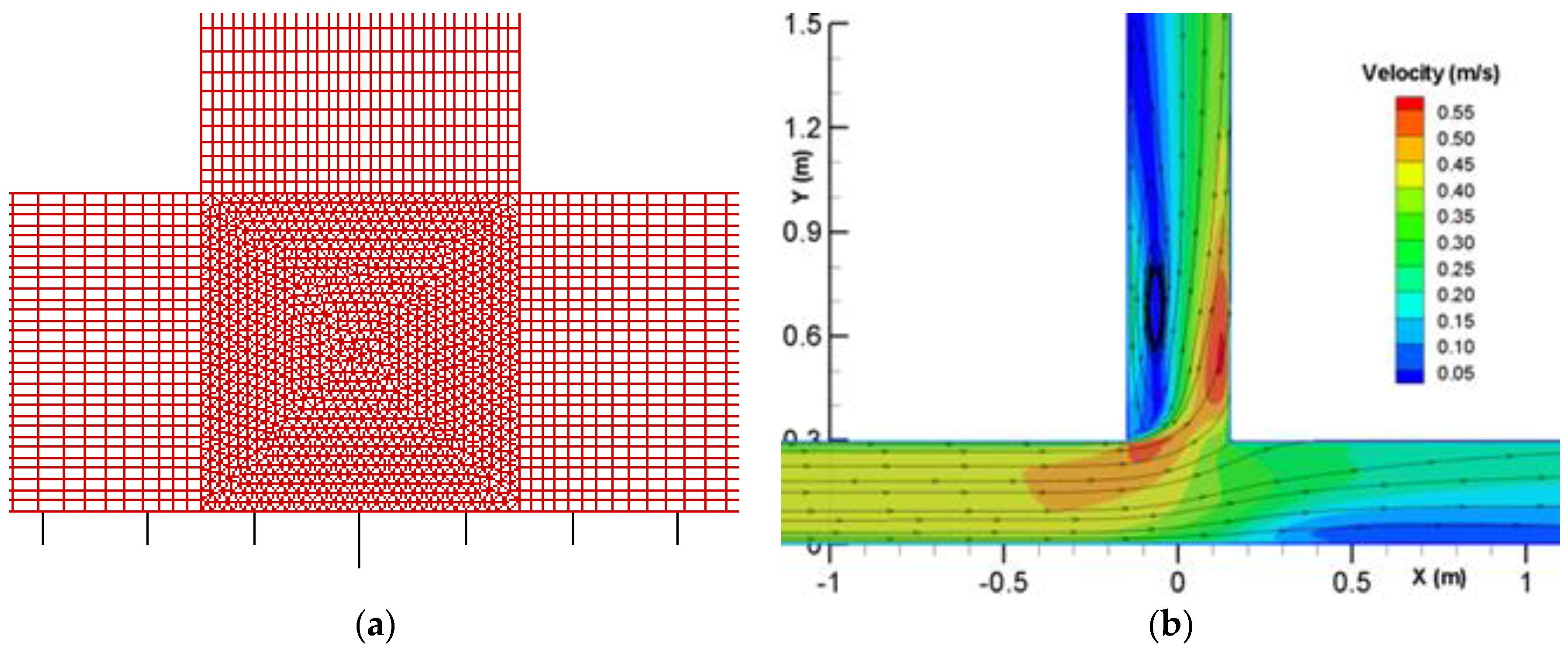
The solution domain consists of a main channel, 6.0 m in length and 0.3 m in width, and a side diversion channel normal to the main channel, 3.0 m in length and 0.3 m in width. Two horizontal meshes are used: one is the same as the 2D mesh of [13], which used pure quadrilaterals, and the other adopts the triangle-quadrilateral hybrid mesh. A total of 16 vertical cells are selected leading to 76,800 cells for the first mesh and 107,280 cells for the mixed mesh. A close-up view of the mixed mesh is shown in Figure 1a.
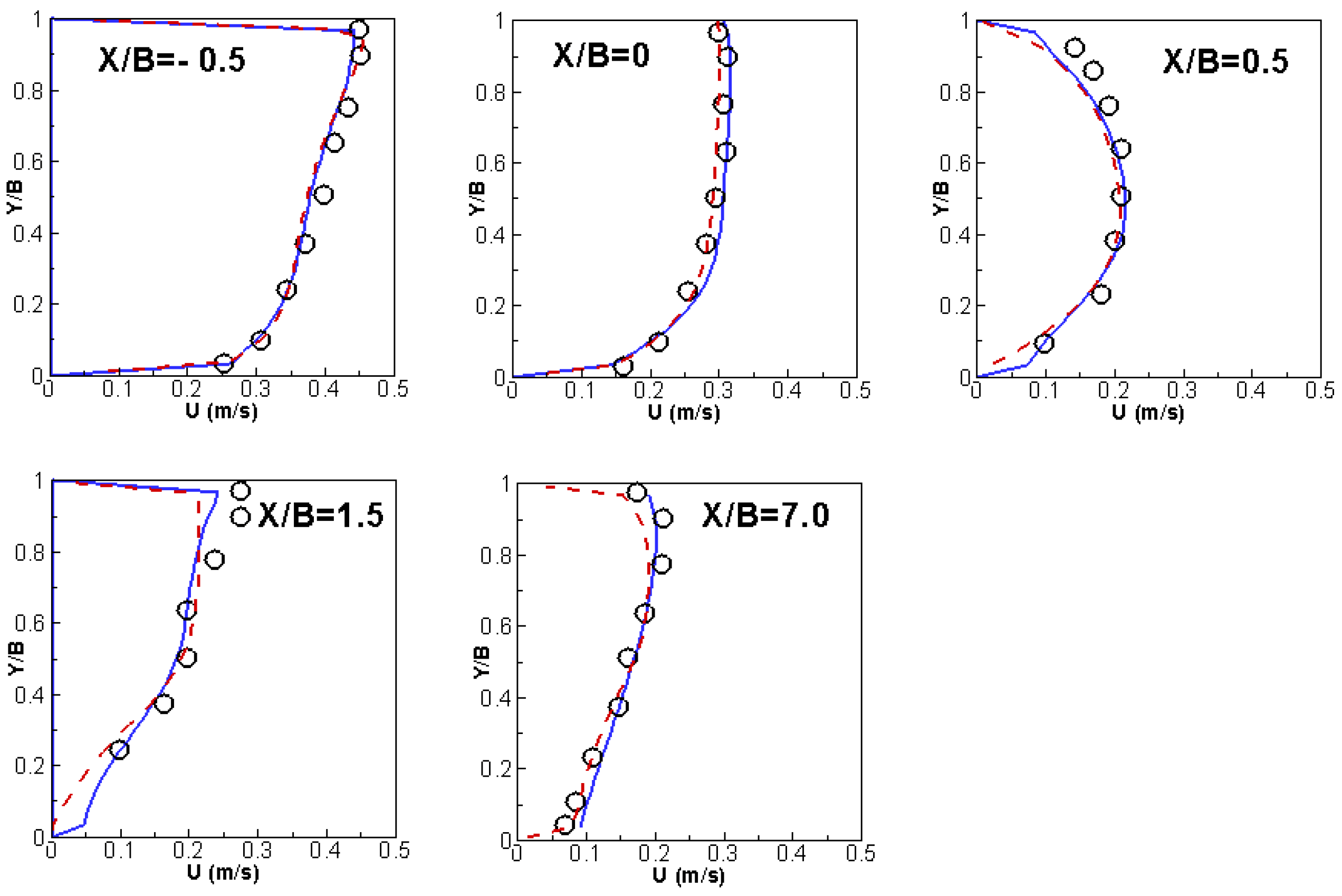
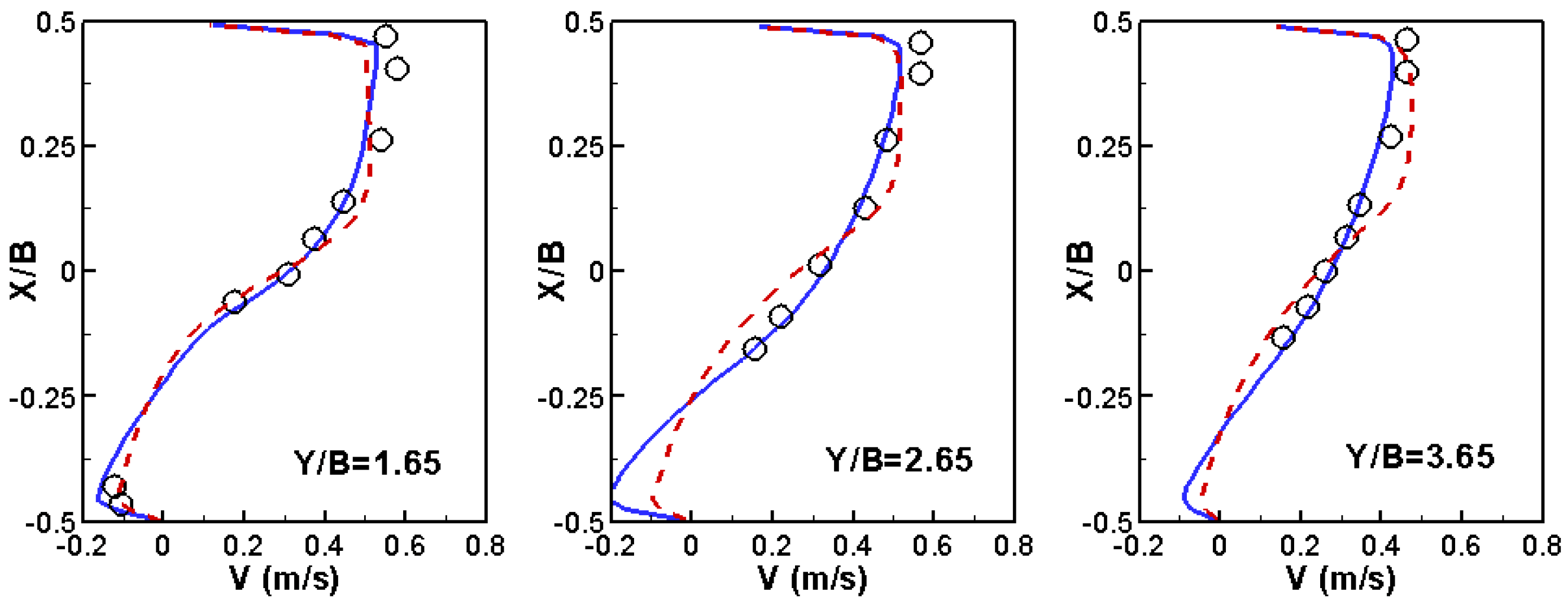
The flow conditions are as follows. The main channel has a discharge of 0.00567 m3/s (applied at X = −3.0 m) and water surface elevation of 0.0555 m at the exit (X = 3.0 m); the water surface elevation is 0.0465 m at the exit of the diversion channel (Y = 3.3 m). The simulation with the two meshes produces essentially the same results, so only results from the mixed mesh are reported herein. The predicted flow pattern is shown in Figure 1b. Key flow features are predicted well, such as flow acceleration near the junction and into the diversion channel and the flow recirculation in the diversion channel. Simulated results are compared with the measured data of [44]; the water surface elevation is in Figure 2 and the depth-averaged velocity is in Figure 3 and Figure 4 in both the main and side channels. Good agreements are obtained between the model results and the data. The SRH-3D and SRH-2D results are similar, which points to the fact that 2D models are applicable for such flows, at least for the case simulated.
5.2. Flow in a Sharply Curved Bend
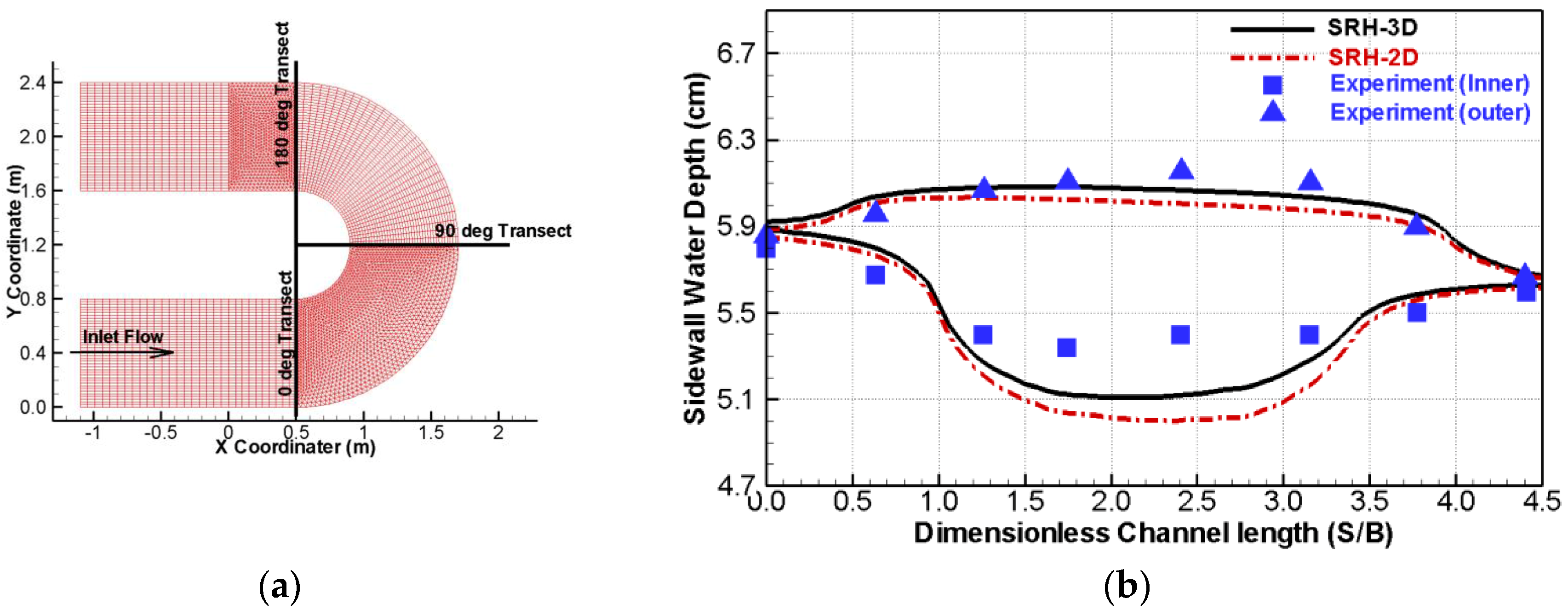
An open channel flow with a sharp 180° rectangular bend was experimentally studied in [45]. A bend with a mean radius-to-width ratio of 3.0 and less is considered strongly curved and exhibits highly 3D flow characteristics [46]. The Rozovskii bend has a mean radius-to-width ratio of 1.0, so it belongs to the very sharp bend category. The same case was subject to a number of numerical studies, such as a 2D depth-averaged modeling in [46], a 2D modeling explicitly taking into account the secondary flow in [47], and a 3D NS solver modeling in [48].
The model domain and bed geometry are shown in Figure 5a. The approach and exit channels are straight, 1.6 m in length, and 0.8 m in width. The bend has a radius of 0.4 m for the inner wall. The numerical modeling parameters are as follows. The entire channel has a flat smooth bottom. The discharge at the entrance is 0.0123 m3/s, resulting in an average velocity of 0.265 m/s, Reynolds number of 15,600, and Froude number of 0.11. The water elevation at the model exit is extrapolated from the experimental data. The horizontal mesh adopts the mixed triangles (two zones) and quadrilaterals (Figure 5a). A total of 20 vertical mesh cells are chosen, leading to a total of 165,280 3D mesh cells.
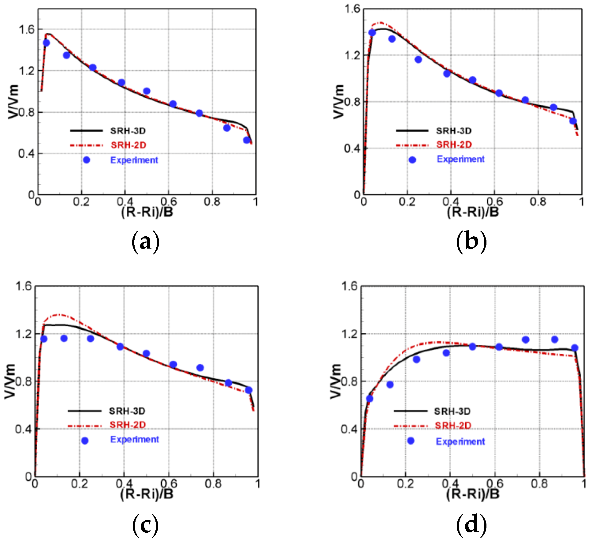
Predicted water depth along the inner and outer sidewall is compared with the experimental data in Figure 5b. It is seen that the water surface elevation is higher at the outer bank than at the inner bank—the expected super-elevation effect. The model results match well along the outer wall and the elevation is under-predicted along the inner wall. The SRH-3D model indeed has a better prediction than the 2D model, indicating that vertical variation of the velocity and the secondary flow produced by the sharp bend have some effects on the flow.
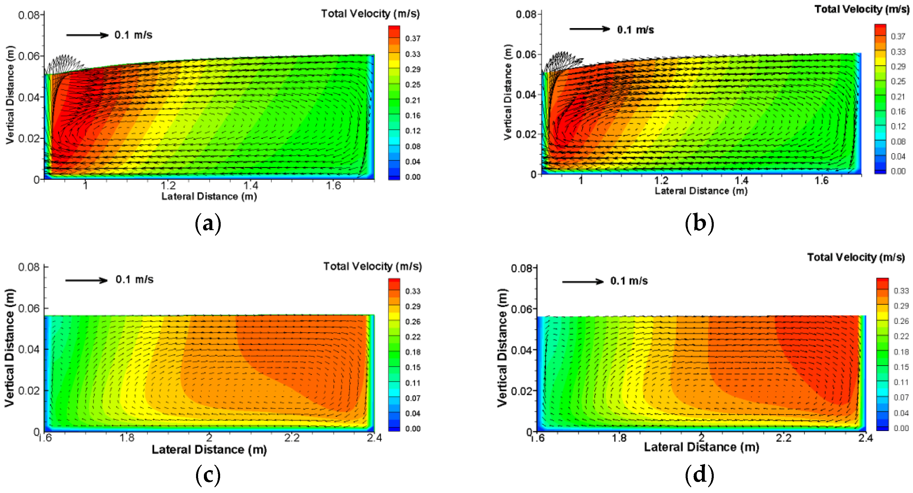
Predicted depth-averaged velocity is compared with the experimental data in Figure 6. The 3D model results agree with the measured data well. It is noted that the 2D model results agree also well with the data, contrary to the finding of [47]. The improvements of the 3D model over the 2D are mainly in the shift of the maximum velocity from the inner to outer sidewalls when flow comes out of the bend. This rapid shift can be explained by the falling transverse water elevation slope and release of the additional momentum by the secondary flow when the radius of curvature at the bend exit abruptly changes to infinity. Finally, the ability of SRH-3D model to predict secondary flows is examined, since primary reasons to use a 3D model are to predict vertical velocity distribution and secondary flows. There is no secondary flow data with the present case, so a separate simulation using the NS solver U2RANS [43] is carried out. Comparison of the predicted secondary flows at two transects are compared in Figure 7 between SRH-3D and U2RANS. Very similar secondary flows are predicted by the two models. This shows the hydrostatic models, such as SRH-3D, are adequate in predicting the secondary flows, even in sharp bends.
5.3. Suspended Sediment in a Channel
3D modeling of suspended sediment transport is not trivial; correct implementation of even the bed boundary condition is not well understood [37]. The flume results in [49] are used to test the sediment module. The experiment was carried out in a flume with rough bottom created by placing a single layer of pebble-sized stones (median diameter: 7 mm). The bed slope was 0.07252%. The water elevation from the roughened bottom was 62 mm after the flow was fully developed. A log-fit of the measured velocity profile led to the shear velocity of m. The mean velocity was 0.22 m/s. The mesh has 62 cells along the 12.4 m flow direction and 31 vertical cells distributed non-uniformly. The cell center of the first cell near the bed is mm, so that the point is within the log law (). Upstream discharge is 0.01364 m3/s, downstream depth is 62 mm, and bed roughness height is = 13 mm.
The computed velocity and vertical eddy viscosity distribution are compared with the experimental data in Figure 8. Good agreement is obtained. Vertical eddy viscosity is important in predicting the suspended sediment transport. For the present case, two mechanisms are important for the sediment motion: settling velocity and turbulent resuspension. The well-cited experimental data sets of [50,51] are used for comparison of the turbulent viscosity.
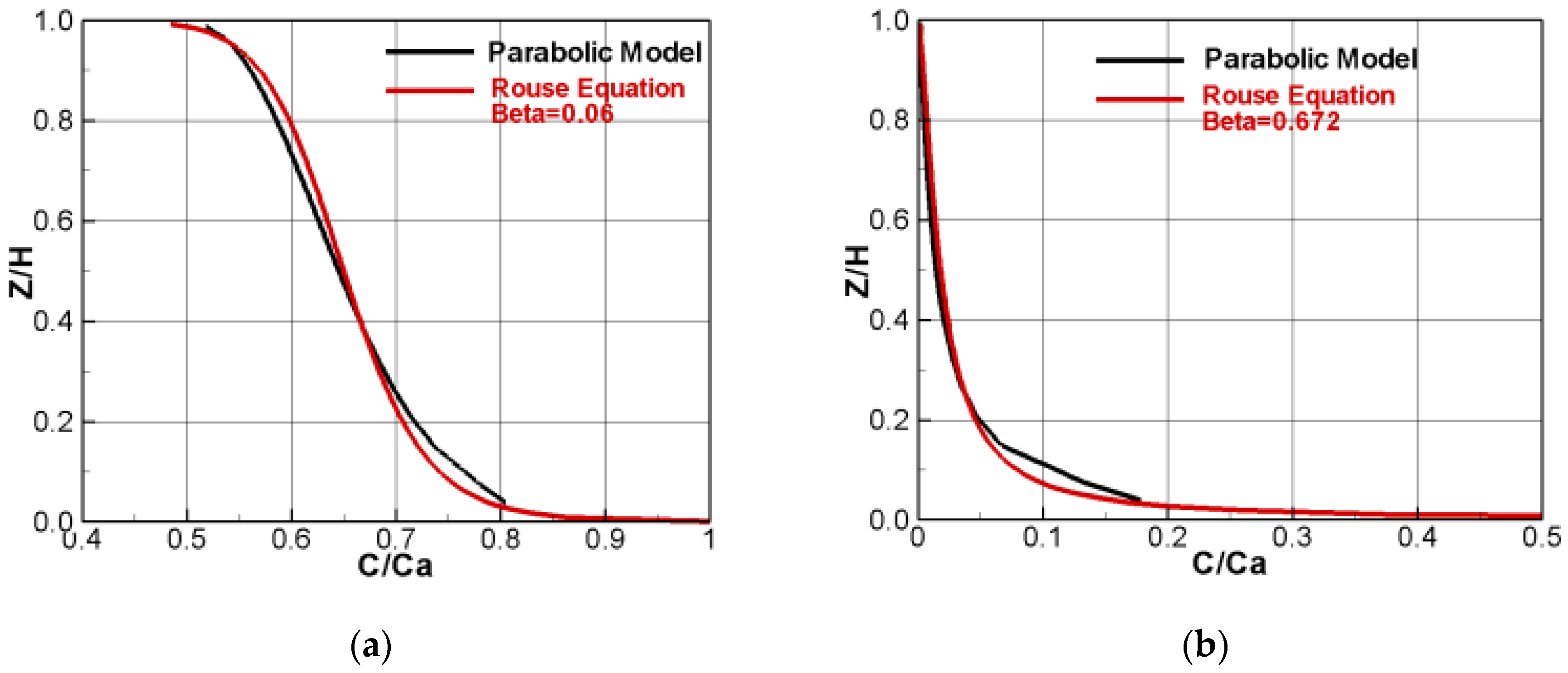
Two model runs are made to compute the suspended sediment corresponding to two sediment sizes. The same runs were reported by [37]. Run 1 has a sediment size of 0.0236 mm, sediment fall velocity of 0.0516 mm/s, and Rouse number of 0.06. Run 2 has the sediment diameter of 0.079 mm, fall velocity of 5.79 mm/s, and the Rouse number of 0.672. The sediment sizes are chosen, such that the Rouse parameters are significantly different. The simulation starts from clear water and stops once the equilibrium sediment concentration profiles are obtained. Predicted concentration is compared with the theoretical Rouse profile in Figure 9. It is seen that the Rouse profile is well predicted by the model. Note that the Rouse profile is only approximate and was derived by assuming the parabolic distribution of the vertical turbulence viscosity.
5.4. Lock Exchange: Intrusive Turbidity Current into a Two-layer Fluid
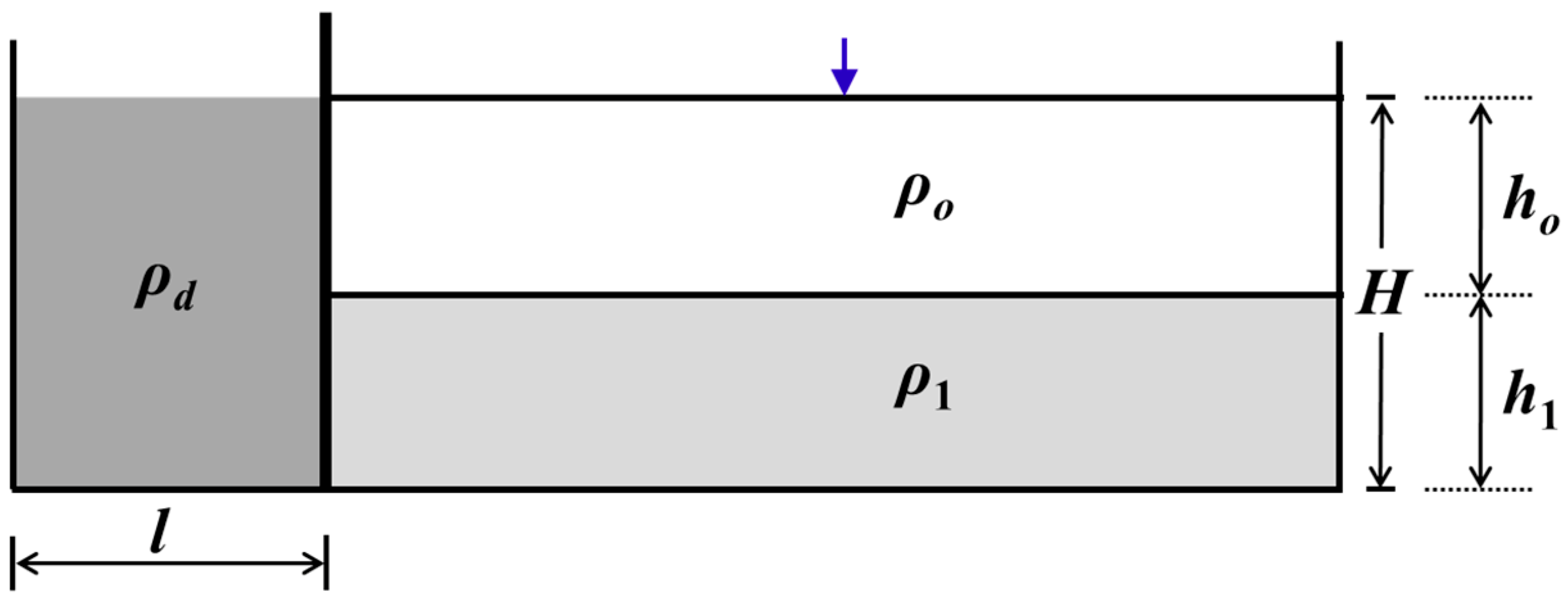
Intrusion of a turbidity current into a two-layer fluid is simulated next in an attempt to verify the ability of the model to simulate the sediment transport and capture the fluid-sediment interface. The experimental cases of [52] are chosen and the setup is illustrated in Figure 10. The case was also studied by [53] with an NS solver. The flume had a glass tank measuring 197.1 cm long, 19.9 cm wide, and 48.5 cm tall. The lock-length (l) behind the gate was fixed at 18.6 cm and the total water depth (H) was 20 cm.
Two cases are simulated. The first is the symmetric flow turbidity current (SFTC), in which the depth of the two layers in the ambient fluids is equal ( cm). The densities of the two layers are: = 1000 kg/m3 and = 1020 kg/m3. SFTC has the symmetrical flow type according to [52], as the density of the lock fluid is equal to the depth-weighted average of the upper and lower layers. The second case is an asymmetric flow turbidity current (AFTC), in which the depth of the two layers in the ambient fluids are set as = 17.5 cm and = 2.5 cm, respectively. The densities of the two layers are the same as in the first case.
In the numerical modeling, no variations are expected in the lateral direction (y), so only 3 lateral cells are used with the symmetry boundary condition specified in the lateral back and front boundaries. In the two other directions, 533 cells are in the longitudinal direction (x) and 50 cells are in the vertical direction (z). Initially, fluid is stationary. For the SFTC case, the initial concentration is C = 0.006061 in the lock, C = 0.0 and 0.012122 in the top and bottom of the ambient, respectively. For the AFTC case, C = 0.009091 in the lock, and C = 0.0 and 0.012122 in the top and bottom of the ambient, respectively.
The SFTC case results are shown in Figure 11 to visualize the temporal evolution of the intrusive gravity current. They are compared with the images taken from the laboratory experiments of [52]. After the lock gate was removed, the fluid contained behind the lock gate collapsed symmetrically and propagated along the interface. The head already started to form and was visible at 2 s. The initial collapse began with rapid acceleration. As it propagated to the right end of the wall, the gravity current brought strong mixing, resulting in mass entrainment and dilution. These processes are predicted by the numerical model well. The results, however, confirm the finding of [54] that the hydrostatic models, such as the current one, failed to predict the formation of the Kelvin-Helmholtz billows. The present model otherwise is capable of predicting the overall turbidity current features, as well as the propagation speed of the current.
Simulated results of the AFTC case are shown in Figure 12; the temporal evolution of the intrusive gravity current is compared between the model and the experiment of [52]. Similar to the findings of the SFTC case, the hydrostatic model predicts the initial turbidity current formation and travel well. The model, however, is incapable of predicting the Kelvin-Helmholtz waves as well as the wave reflection process after the front reaches the end wall.
6. Conclusions
A new 3D hydrostatic numerical model is developed that may be used to simulate flow and suspended sediment transport in rivers and reservoirs with free surface and fluid-sediment interface. The new model is formulated in a general way so that it is applicable to a wide range of environmental fluid flows. A new solution algorithm is developed that derives the water elevation equation from the vertical summation of the discretized continuity equation. The resultant elevation correction equation is consistent with the rest of the discretized equations, leading to a robust and stable iterative solver. A major contribution of the present study is the adoption of a new mesh—the horizontal polygonal mesh coupled with the arbitrarily distributed vertical mesh. The 3D mesh is terrain-following and movable vertically to changes in water surface elevation and bed elevation.
The flow solver is verified with two 3D cases having experimental data. The model performs well in stability and accuracy. The sharply curved bend flow modeling shows that the 3D hydrostatic model works well for flows in meander bends, as the predicted secondary flows match that from the non-hydrostatic NS solvers. In comparison with the 2D model, the 3D model improves upon the flow through the sharp bend. A primary advantage of the 3D model over 2D ones is that the vertical distribution and secondary flows are predicted.
The suspended sediment transport module is fully coupled to the flow solver, in that the flow dictates the sediment movement and the changes of sediment concentration alter the flow velocity. The coupling is achieved implicitly within the same time step. The sediment module is first tested for its ability to predict the vertical distribution of the sediment concentration, and then used to predict the turbidity current formation and travel. Despite the inability of the model to predict the waves associated with the Kelvin-Helmholtz instability, the model is adequate in predicting the sediment collapse, current formation and movement speed.
Future works include: (a) demonstration and application of SRH-3D to practical rivers; (b) development of the adaptive mesh movement capability to track density interface; and (c) extension to bedload sediment transport.
Author Contributions
Conceptualization, Y.L.; methodology, Y.L.; software, Y.L.; validation, Y.L. and K.W.; investigation, Y.L. and K.W.; resources, Y.L. and K.W.; writing—original draft preparation, Y.L.; writing—review and editing, K.W.
Funding
This research was funded by U.S. Bureau of Reclamation Science and Technology Program and Water Resources Agency of Taiwan.
Conflicts of Interest
The authors declare no conflict of interest.
References
- Gibson, S.; Brunner, G.; Piper, S.; Jensen, M. Sediment Transport Computations in HEC-RAS. In Proceedings of the Eighth Federal Interagency Sedimentation Conference (8thFISC), Reno, NV, USA, 2–6 April 2006; pp. 57–64. [Google Scholar]
- MIKE 11. Users Manual; Danish Hydraulic Institute: The Hague, The Netherlands, 2005. [Google Scholar]
- Wu, W.; Vieira, D.A. One-Dimensional Channel Network Model CCHE1D Version 3.0.—Technical Manual; Technical Report No. NCCHE-TR-2002-1; National Center for Computational Hydroscience and Engineering, The University of Mississippi: Oxford, MS, USA, 2002. [Google Scholar]
- Huang, J.; Greimann, B.P. GSTAR-1D, General Sediment Transport for Alluvial Rivers—One Dimension; Technical Service Center, U.S. Bureau of Reclamation: Denver, CO, USA, 2007.
- Wu, W. Depth-averaged two-dimensional numerical modeling of unsteady flow and non-uniform sediment transport in open channels. J. Hydraul. Eng. 2004, 130, 1013–1024. [Google Scholar] [CrossRef]
- Hung, M.C.; Hsieh, T.Y.; Wu, C.H.; Yang, J.C. Two-dimensional nonequilibrium noncohesive and cohesive sediment transport model. J. Hydraul. Eng. 2009, 135, 369–382. [Google Scholar] [CrossRef]
- Huang, W.; Cao, Z.; Pender, G.; Liu, Q.; Carling, P. Coupled flood and sediment transport modelling with adaptive mesh refinement. Sci. China Technol. Sci. 2015, 58, 1425–1438. [Google Scholar] [CrossRef] [Green Version]
- Jia, Y.; Wang, S.S.Y. CCHE2D: Two-Dimensional Hydrodynamic and Sediment Transport Model for Unsteady Open Channel Flows Over Loose Bed; NCCHE Technical Report, No. NCCHETR-2001-01; The University of Mississippi: Oxford, MS, USA, 2001. [Google Scholar]
- Hervouet, J.-M. Hydrodynamics of Free Surface Flows; John Wiley&Sons, Ltd.: Hoboken, NJ, USA, 2007; pp. 1–360. [Google Scholar]
- Casulli, V.; Walters, R.A. An unstructured grid, three dimensional model based on the shallow water equations. Int. J. Numer. Meth. Fluids 2000, 32, 331–348. [Google Scholar] [CrossRef]
- Bever, A.J.; MacWilliams, M.L. Simulating sediment transport processes in San Pablo Bay using coupled hydrodynamic, wave, and sediment transport models. Mar. Geol. 2013, 345, 235–253. [Google Scholar] [CrossRef]
- Deltares. Delft3D-FLOW. Simulation of multi-dimensional hydrodynamic flow and transport phenomena, including sediments—User Manual; Version 3.04, rev. 11114; Deltares: Delft, The Netherlands, 2010. [Google Scholar]
- Lai, Y.G. SRH-2D Version 2: Theory and User’s Manual; Technical Service Center, U.S. Bureau of Reclamation: Denver, CO, USA, 2008.
- Lai, Y.G. Two-Dimensional Depth-Averaged Flow Modeling with an Unstructured Hybrid Mesh. J. Hydraul. Eng. 2010, 136, 12–23. [Google Scholar] [CrossRef]
- Paik, J.; Eghbalzadeh, A.; Sotiropoulos, F. Three-Dimensional Unsteady RANS Modeling of Discontinuous Gravity Currents in Rectangular Domains. J. Hydraul. Eng. 2009, 135, 505–521. [Google Scholar] [CrossRef]
- Papanicolaou, A.N.T.; Elhakeem, M.; Krallis, G.; Prakash, S.; Edinger, J. Sediment Transport Modeling Review—Current and Future Developments. J. Hydraul. Eng. 2008, 134, 1–14. [Google Scholar] [CrossRef]
- Blumberg, A.F.; Mellor, G.L. Diagnostic and prognostic numerical circulation studies of the south Atlantic bight. J. Geophys. Res. 1983, 88, 4579–4592. [Google Scholar] [CrossRef]
- Blumberg, A.F.; Mellor, G.L. A description of a three-dimensional coastal ocean circulation model. In Three-Dimensional Coastal Ocean Models, Coastal and Estuarine Science; Heaps, N.S., Ed.; American Geophysical Union: Washington, DC, USA, 1987; Volume 4, pp. 1–19. [Google Scholar]
- HydroQual, Inc. A primer for ECOMSED: Users Manual; HydroQual, Inc.: Mahwah, NJ, USA, 2002. [Google Scholar]
- Hamrick, J.M. A Three-Dimensional Environmental Fluid Dynamics Computer Code: Theoretical and Computational Aspects; Special Report 317; The College of William and Mary, Virginia Institute of Marine Science: Gloucester Point, VA, USA, 1992; 63p. [Google Scholar]
- DHI. Delft3D-FLOW: Simulation of Multi-Dimensional Hydrodynamic Flows and Transport Phenomena, Including Sediments; Deltares: Delft, The Netherlands, 2011. [Google Scholar]
- Roelvink, J.A.; van Banning, G.K.F.M. Design and development of DELFT3D and application to coastal morphodynamics. In Hydroinformatics; Verwey, A., Minns, A.W., Babovic, V., Maksimovic, C., Eds.; Balkema: Rotterdam, The Netherlands, 1994; pp. 451–456. [Google Scholar]
- Lesser, G.R. Computation of Three-Dimensional Suspended Sediment Transport within the DELFT3D-FLOW Module; WLjDelft Hydraulics Report Z2396; Delft Hydraulics: Delft, The Netherlands, 2000. [Google Scholar]
- Johnson, B.H.; Kim, K.W.; Heath, R.E.; Hsieh, B.B.; Butler, H.L. Validation of three dimensional hydrodynamic model of Chesapeake Bay. J. Hydraul. Eng. 1993, 119, 2–20. [Google Scholar] [CrossRef]
- Spasojevic, M.; Holly, F.M. Three-Dimensional Numerical Simulation of Mobile-Bed Hydrodynamics; Contract Rep. HL-94-2; U.S. Army Engineer Waterways Experiment Station: Vicksburg, MS, USA, 1994. [Google Scholar]
- Gessler, D.; Hall, B.; Spasojevic, M.; Holly, F.M.; Pourtaheri, H.; Raphelt, N.X. Application of 3D mobile bed, hydrodynamics model. J. Hydraul. Eng. 1999, 125, 737–749. [Google Scholar] [CrossRef]
- Haidvogel, D.B.; Arango, H.; Budgell, W.P.; Cornuelle, B.D.; Curchitser, E.; Di Lorenzo, E.; Fennel, K.; Geyer, W.R.; Hermann, A.J.; Lanerolle, L. Ocean forecasting in terrain-following coordinates: Formulation and skill assessment of the Regional Ocean Modeling System. J. Comput. Phys. 2008, 227, 3595–3624. [Google Scholar] [CrossRef]
- Moriarty, J.M.; Harris, C.K.; Hadfield, M.G. A Hydrodynamic and Sediment Transport Model for the Waipaoa Shelf, New Zealand: Sensitivity of Fluxes to Spatially-Varying Erodibility and Model Nesting. J. Mar. Sci. Eng. 2014, 2, 336–369. [Google Scholar] [CrossRef] [Green Version]
- Leendertse, J.J. Turbulence modelling of surface water flow and transport: Part IVa. J. Hydr. Eng. 1990, 114, 603–606. [Google Scholar] [CrossRef]
- Stelling, G.S.; van Kester, J.A. On the approximation of horizontal gradients in sigma co-ordinates for bathymetry with steep bottom slopes. Int. J. Numer. Meth. Fluids 1994, 18, 915–955. [Google Scholar] [CrossRef]
- Bijvelds, M.D.J.P. Numerical Modelling of Estuarine Flow over Steep Topography; Delft University of Technology: Delft, The Netherlands, 2001; 136p. [Google Scholar]
- Cornelissen, S.C. Numerical Modelling of Stratified Flows Comparison of the Sigma and z Coordinate Systems. Master’s Thesis, Delft University of Technology, Delft, The Netherlands, 2004; 94p. [Google Scholar]
- Mandang, I.; Yanagi, T. Cohesive sediment transport in the 3D hydrodynamic baroclinic circulation model in the Mahakam Estuary, East Kalimantan, Indonesia. Coast. Mar. Sci. 2009, 32, 1–13. [Google Scholar]
- Rodi, W. Turbulence models and their application in Hydraulics, State-of-the-art paper article sur l’etat de connaissance. In Proceedings of the IAHR Sectionon Fundamentals of Division II: Experimental and Mathematical Fluid Dynamics, Delft, The Netherlands, 3–6 September 1984. [Google Scholar]
- Celik, I.; Rodi, W. Modeling suspended sediment transport in nonequilibrium situations. J. Hydraul. Eng. 1988, 114, 1157–1191. [Google Scholar] [CrossRef]
- Van Rijn, L.C. Principles of Sediment Transport in Rivers, Estuaries and Coastal Seas; Aqua Publications: Amsterdam, The Netherlands, 1993. [Google Scholar]
- Liu, X. New Near-Wall Treatment for Suspended Sediment Transport Simulations with High Reynolds Number Turbulence Models. J. Hydraul. Eng. 2014, 140, 333–339. [Google Scholar] [CrossRef]
- Fredsøe, J.; Andersen, K.H.; Sumer, B.M. Wave plus current over ripple-covered bed. Coast. Eng. 1999, 38, 117–221. [Google Scholar] [CrossRef]
- Garcia, M.H.; Parker, G. Entrainment of Bed Sediment into Suspension. J. Hydraul. Eng. 1991, 117, 414–435. [Google Scholar] [CrossRef]
- Garcia, M.H. (Ed.) ASCE Manuals and Reports on Engineering Practice No. 110, Sedimentation Engineering: Processes, Measurements, Modeling, and Practice; ASCE: Reston, VA, USA, 2008. [Google Scholar]
- Zyserman, J.; Fredsøe, J. Data Analysis of Bed Concentration of Suspended Sediment. J. Hydraul. Eng. 1994, 120, 1021–1042. [Google Scholar] [CrossRef]
- Lai, Y.G.; Przekwas, A.J. A Finite-Volume Method for Simulations of Fluid Flows with Moving Boundaries. Int. J. Comp. Fluid Dyn. 1994, 2, 19–40. [Google Scholar] [CrossRef]
- Lai, Y.G.; Weber, L.J.; Patel, V.C. Non-hydrostatic three dimensional method for hydraulic flow simulation. I: Formulation and verification. J. Hydraul. Eng. 2003, 129, 196–205. [Google Scholar] [CrossRef]
- Shettar, A.S.; Murthy, K.K. A numerical study of division of flow in open channels. J. Hydraul. Res. 1996, 34, 651–675. [Google Scholar] [CrossRef]
- Rozovskii, I.L. Flow of Water in Bends of Open Channels; The Israel Program for Scientific Translations: Jerusalem, Israel, 1961. [Google Scholar]
- Molls, T.; Chaudhry, M.H. Depth-averaged open-channel flow model. J. Hydraul. Eng. 1995, 121, 453–465. [Google Scholar] [CrossRef]
- Lien, N.C.; Hsieh, T.Y.; Yang, J.C.; Yeh, K.C. Bed-flow simulation using 2D depth-averaged model. J. Hydraul. Eng. 1999, 125, 1097–1108. [Google Scholar] [CrossRef]
- Leschziner, M.A.; Rodi, W. Calculation of strongly curved open channel flow. J. Hydraul. Div. 1979, 105, 1297–1314. [Google Scholar]
- Fuhrman, D.R.; Dixen, M.; Jacobsen, N.G. Physically-consistent wall boundary conditions for the k-omega turbulence model. J. Hydraul. Res. 2010, 48, 793–800. [Google Scholar] [CrossRef]
- Ueda, H.; Moller, R.; Komori, S.; Mizushina, T. Eddy diffusivity near the free surface of open channel flow. Int. J. Heat Mass Transf. 1977, 20, 1127–1136. [Google Scholar] [CrossRef]
- Nezu, I.; Rodi, W. Open-channel flow measurements with a laser doppler anemometer. J. Hydraul. Eng. 1986, 112, 335–355. [Google Scholar] [CrossRef]
- Sutherland, B.R.; Kyba, P.J.; Flynn, M.R. Intrusive Gravity Currents in Two-layer Fluids. J. Fluid Mech. 2004, 514, 327–353. [Google Scholar] [CrossRef]
- An, S.D. Interflow Dynamics and Three-Dimensional Modeling of Turbid Density Currents in Imha Reservoir, South Korea. Ph.D. Thesis, Department of Civil and Environmental Engineering, Colorado State University, Fort Collins, CO, USA, 2011. [Google Scholar]
- Fringer, O.B.; Gerritsen, M.G.; Street, R.L. An Unstructured-grid, Finite-Volume, Nonhydrostatic, Parallel Coastal Ocean Simulator. Ocean Model. 2006, 14, 139–173. [Google Scholar] [CrossRef]
Figure 1.
A portion of the mixed mesh at the juncture (a) and the predicted surface flow velocity for the flow diversion case (b).
Figure 1.
A portion of the mixed mesh at the juncture (a) and the predicted surface flow velocity for the flow diversion case (b).

Figure 2.
Comparison of water elevation along both walls of the main channel (a) and the side channel (b).
Figure 2.
Comparison of water elevation along both walls of the main channel (a) and the side channel (b).

Figure 3.
Comparison of x-velocity profiles at selected x locations in the main channel (Solid Blue Line: SRH-3D; Red Dashed Line: SRH-2D; Symbol: Experiment).
Figure 3.
Comparison of x-velocity profiles at selected x locations in the main channel (Solid Blue Line: SRH-3D; Red Dashed Line: SRH-2D; Symbol: Experiment).

Figure 4.
Comparison of V velocity profiles at selected y locations in the side channel (Solid Blue Line: SRH-3D; Red Dashed Line: SRH-2D; Symbol: Experiment).
Figure 4.
Comparison of V velocity profiles at selected y locations in the side channel (Solid Blue Line: SRH-3D; Red Dashed Line: SRH-2D; Symbol: Experiment).

Figure 5.
Model domain and the horizontal mixed mesh (a) and a comparison of the water depth along the inner and outer sidewall for the bend case (b).
Figure 5.
Model domain and the horizontal mixed mesh (a) and a comparison of the water depth along the inner and outer sidewall for the bend case (b).

Figure 6.
Comparison of simulated depth-averaged velocity (normalized by the average velocity) across the channel width at four transects for the bend case. (a) 35°; (b) 100°; (c) 143°; (d) 186°.
Figure 6.
Comparison of simulated depth-averaged velocity (normalized by the average velocity) across the channel width at four transects for the bend case. (a) 35°; (b) 100°; (c) 143°; (d) 186°.

Figure 7.
Comparison of predicted secondary flows: SRH-3D on the left and U2RANS on the right. (a) SRH-3D at transect 90°; (b) U2RANS at transect 90°; (c) SRH-3D at transect 0.1 m after exit; (d) U2RANS at transect 0.1 m after exit.
Figure 7.
Comparison of predicted secondary flows: SRH-3D on the left and U2RANS on the right. (a) SRH-3D at transect 90°; (b) U2RANS at transect 90°; (c) SRH-3D at transect 0.1 m after exit; (d) U2RANS at transect 0.1 m after exit.

Figure 8.
Comparison of predicted results with the measured data for the Fuhrman case. (a) velocity; (b) turbulent viscosity.
Figure 8.
Comparison of predicted results with the measured data for the Fuhrman case. (a) velocity; (b) turbulent viscosity.

Figure 9.
Comparison of suspended sediment concentration vertical distribution for the Fuhrman case (Black line: the model; Red line: Rouse equation). (a) Run 1; (b) Run 2.
Figure 9.
Comparison of suspended sediment concentration vertical distribution for the Fuhrman case (Black line: the model; Red line: Rouse equation). (a) Run 1; (b) Run 2.

Figure 10.
Sketch and parameters for the intrusive gravity current cases.

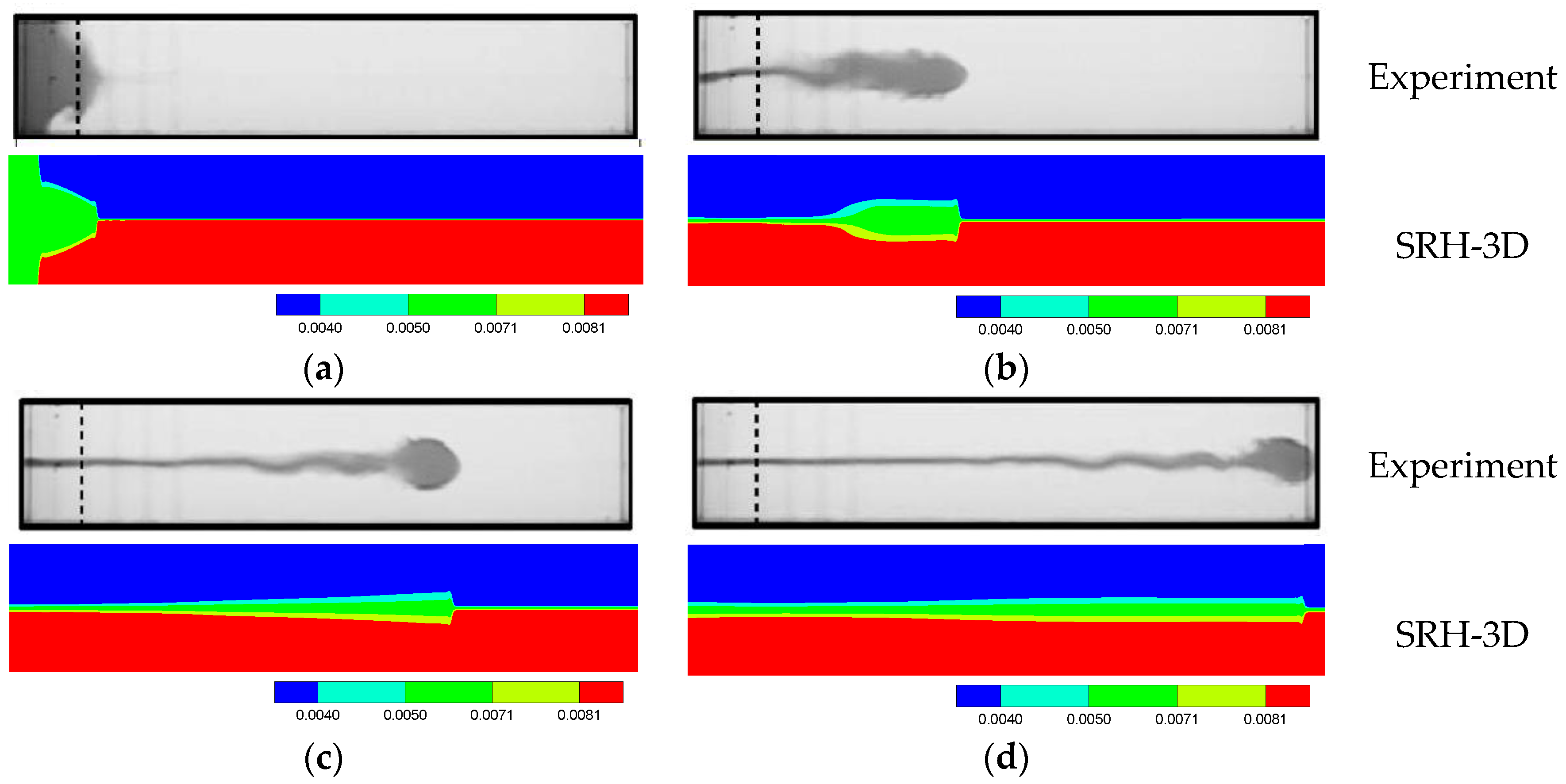
Figure 11.
Temporal evolution of the SFTC intrusive gravity current—sediment concentration contours. Experiment is from [52] and visualized by adding dye. (a) Time = 2 s; (b) Time = 14 s; (c) Time = 26 s; (d) Time = 38 s.
Figure 11.
Temporal evolution of the SFTC intrusive gravity current—sediment concentration contours. Experiment is from [52] and visualized by adding dye. (a) Time = 2 s; (b) Time = 14 s; (c) Time = 26 s; (d) Time = 38 s.

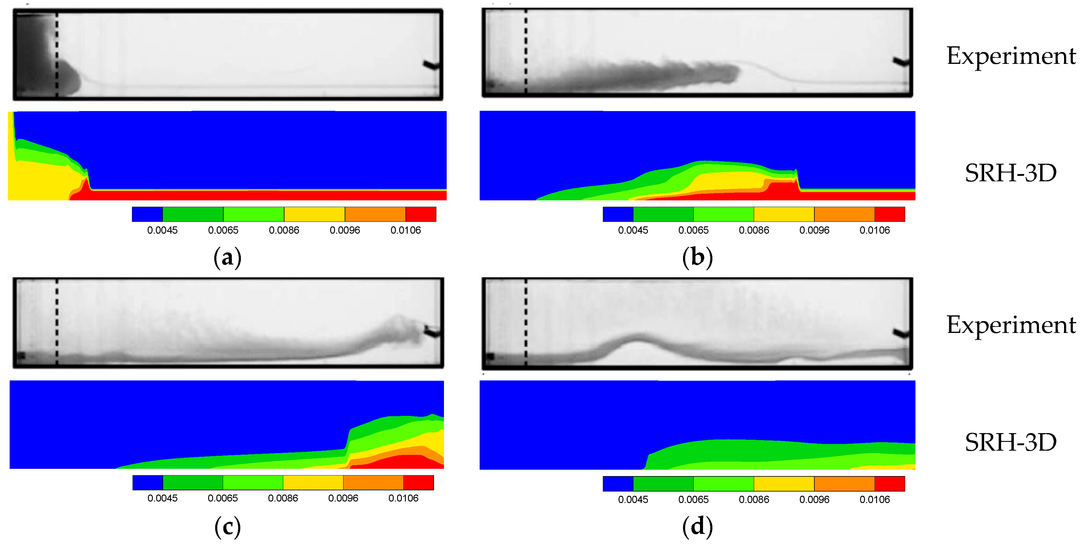
Figure 12.
Temporal evolution of the AFTC intrusive gravity current—sediment concentration contours. Experiment is from [52] and visualized by adding dye. (a) Time = 2 s; (b) Time = 14 s; (c) Time = 26 s; (d) Time = 38 s.
Figure 12.
Temporal evolution of the AFTC intrusive gravity current—sediment concentration contours. Experiment is from [52] and visualized by adding dye. (a) Time = 2 s; (b) Time = 14 s; (c) Time = 26 s; (d) Time = 38 s.

© 2019 by the authors. Licensee MDPI, Basel, Switzerland. This article is an open access article distributed under the terms and conditions of the Creative Commons Attribution (CC BY) license (http://creativecommons.org/licenses/by/4.0/).
Share and Cite
MDPI and ACS Style
Lai, Y.G.; Wu, K. A Three-Dimensional Flow and Sediment Transport Model for Free-Surface Open Channel Flows on Unstructured Flexible Meshes. Fluids 2019, 4, 18. https://doi.org/10.3390/fluids4010018
AMA Style
Lai YG, Wu K. A Three-Dimensional Flow and Sediment Transport Model for Free-Surface Open Channel Flows on Unstructured Flexible Meshes. Fluids. 2019; 4(1):18. https://doi.org/10.3390/fluids4010018
Chicago/Turabian StyleLai, Yong G., and Kuowei Wu. 2019. "A Three-Dimensional Flow and Sediment Transport Model for Free-Surface Open Channel Flows on Unstructured Flexible Meshes" Fluids 4, no. 1: 18. https://doi.org/10.3390/fluids4010018