
Optimizing Drone-Based Surface Models for Prescribed Fire Monitoring
by
 , , and
Christian Mestre-Runge
1,* ,
,
Marvin Ludwig
2,
Maria Teresa Sebastià
3,
Josefina Plaixats
4 and
Agustin Lobo
5 1
Department of Biology, University of Marburg, 35043 Marburg, Germany
2
Institute of Landscape Ecology, University of Münster, 48149 Münster, Germany
3
Laboratory ECOFUN, Forest Science and Technology Centre of Catalonia (CFTC), 25280 Solsona, Spain
4
Grup de Recerca en Remugants, Departament de Ciència Animal i dels Aliments, Universitat Autònoma de Barcelona, 08193 Bellaterra, Spain
5
Geoscience Barcelona (GEO3BCN-CSIC), 08028 Barcelona, Spain
*
Author to whom correspondence should be addressed.
Fire 2023, 6(11), 419; https://doi.org/10.3390/fire6110419
Submission received: 26 September 2023
/
Revised: 19 October 2023
/
Accepted: 25 October 2023
/
Published: 2 November 2023
(This article belongs to the Special Issue Drone Applications Supporting Fire Management)
Abstract
:Prescribed burning and pyric herbivory play pivotal roles in mitigating wildfire risks, underscoring the imperative of consistent biomass monitoring for assessing fuel load reductions. Drone-derived surface models promise uninterrupted biomass surveillance but require complex photogrammetric processing. In a Mediterranean mountain shrubland burning experiment, we refined a Structure from Motion (SfM) and Multi-View Stereopsis (MVS) workflow to diminish biases in 3D modeling and RGB drone imagery-based surface reconstructions. Given the multitude of SfM-MVS processing alternatives, stringent quality oversight becomes paramount. We executed the following steps: (i) calculated Root Mean Square Error (RMSE) between Global Navigation Satellite System (GNSS) checkpoints to assess SfM sparse cloud optimization during georeferencing; (ii) evaluated elevation accuracy by comparing the Mean Absolute Error (MAE) of six surface and thirty terrain clouds against GNSS readings and known box dimensions; and (iii) complemented a dense cloud quality assessment with density metrics. Balancing overall accuracy and density, we selected surface and terrain cloud versions for high-resolution (2 cm pixel size) and accurate (DSM, MAE = 57 mm; DTM, MAE = 48 mm) Digital Elevation Model (DEM) generation. These DEMs, along with exceptional height and volume models (height, MAE = 12 mm; volume, MAE = 909.20 cm3) segmented by reference box true surface area, substantially contribute to burn impact assessment and vegetation monitoring in fire management systems.
1. Introduction
Environmental management practices that integrate prescribed burning (the controlled use of fire in selected vegetation stands) with directed grazing (often referred to as “pyric herbivory”) are gaining traction as means to reduce wildfire risks and foster resilient grassland ecosystems [1,2,3]. Public agencies and environmental authorities are increasingly considering the practical application of these strategies [4].
Both prescribed burning and pyric herbivory are intricate treatments, with their efficacy largely dependent on pivotal elements such as timing and frequency [5]. These interventions must be tailored to the specificities of local environments, underscoring the importance of evaluating their impacts and tracking vegetation changes, especially in the realm of prescribed burning activities.
A vital component of monitoring these treatments is gauging the aboveground biomass (AGB). The dynamics of AGB shed light on the workings of ecosystems [6] and are of particular significance in studies concerning wildfires and prescribed burning, as AGB is a primary factor determining fuel availability.
Direct measurements of AGB can be obtained through field surveys that involve cutting and weighing vegetation [7]. Alternatively, allometric models, which correlate AGB with quantifiable biophysical metrics like canopy height or phytovolume, offer indirect estimations [8,9]. Yet, in landscapes marked by heterogeneity, executing field sampling for AGB, canopy height, and phytovolume becomes challenging due to the extensive sampling points needed [9]. As a result, satellite and mid-tier remote sensing methods, including Light Detection and Ranging (LiDAR) systems, have become popular tools to observe biophysical attributes in rangelands [10,11]. However, conventional imaging often falls short in providing the spatial resolution necessary to effectively depict canopy structures in these areas [12]. Given this limitation, drone imagery is gaining traction as a potent alternative in the realm of prescribed burning research [8,12,13,14,15,16].
UAV flights offer flexibility, allowing for rapid deployment in response to specific events like natural or controlled fires, as well as changes in environmental conditions [17,18]. Their ability to provide high temporal resolution data also makes them suitable for periodic surveys. The use of UAVs equipped with consumer-grade RGB cameras for the generation of Digital Elevation Models (DEMs) is on the rise, primarily because they are cost-effective and tailored for smaller areas, such as plots spanning 5 ha [19].
A DEM provides a digital representation of a topographic surface. It is typically a georeferenced grid that mirrors a specific section of Earth or another solid entity [20]. Broadly speaking, DEMs capture two main surfaces: the Digital Terrain Model (DTM), which portrays the bare ground; and the Digital Surface Model (DSM), which reflects the highest surface, whether that be vegetation or other natural or manmade features [21]. The creation of DEMs involves interpolating dense point clouds, which are formed using photogrammetric techniques such as Structure from Motion (SfM) [22,23,24,25,26,27,28] and Multi-View Stereopsis (MVS) [29,30]. Owing to their utility, DEMs have found applications across various geoscientific domains, including topographic mapping [31,32], geomorphology [33], forestry [34], precision agriculture [35], rangeland management [36], and disaster response [37], to name a few.
Generating a DSM might seem like a direct task, but the setting of MVS parameters for dense surface point cloud reconstruction plays a crucial role in determining DSM quality [38]. One of the enduring challenges is differentiating 3D points that represent vegetation from those indicating terrain, which complicates the classification of Dense Terrain Point Clouds (DTPCs) needed to create a DTM. Numerous filtering techniques and interpolation methods have been explored for this purpose, with varying degrees of success across different applications [39,40,41,42,43,44].
An essential product of this process is the Canopy Height Model (CHM), which provides insight into canopy height variations by subtracting the DTM from the DSM. The combination of UAV technology with RGB cameras and standard SfM-MVS procedures has emerged as a cost-efficient method for producing highly precise and spatially detailed DEMs. This technique has shown effectiveness for a wide range of vegetation types, from 2 cm tall grasses to multi-meter shrubs and trees. Its applications span various environments, including grasslands [7,9,35,44,45], floodplains [46], and dryland shrubberies [41], and it is used for estimating phytovolume in grasslands [36], as well as Mediterranean forests [13].
The effectiveness of DEMs is determined by a plethora of factors throughout the SfM-MVS workflow. These influencing elements range from the design of the experimental flight [47] and camera configurations [48] to the quantity and spread of Ground Control Points (GCPs) [49]. Furthermore, environmental conditions [18], the nature of the land cover [39], chosen SfM processing techniques [50], techniques to filter the point cloud [38,40,41], and interpolation strategies [43] all contribute to the final quality of the DEMs. Even though UAV-based photogrammetric and LiDAR techniques have proven valuable in evaluating the effects of prescribed burns [12,13,14,15,16,33,51,52], there is a noticeable gap in research focusing on the operational and processing nuances of SfM-MVS in producing DEMs under such conditions. This means that our understanding of the quality and applicability of these DEMs remains limited.
In our pursuit to bridge the knowledge gap surrounding DEM generation in the context of prescribed burning, we embarked on a study set against the backdrop of a Mediterranean mountain shrubland, subject to both prescribed burning and pyric herbivory treatments. Through a single UAV flight, we collected RGB images to craft DEMs and associated CHMs.
Our research zeroes in on two key objectives:
- To implement an optimized SfM-MVS process tailored to minimize biases in elevation and height, resulting in high-fidelity surface models with a pixel size of just 2 cm/px, derived from RGB imagery captured during a single UAV flight.
- To delve into the ramifications of different SfM-MVS processing permutations on the quality of the 3D models and surface reconstructions, shedding light on the merits and limitations of our chosen optimization strategy.
Our work holds significant sway in this arena by placing a strong emphasis on the quality of surface models—a factor that directly influences our prowess in gauging post-fire vegetation shifts and recovery dynamics, as well as ascertaining the efficacy of interventions like controlled burns and pyric herbivory. This is of paramount importance in protected areas, such as the Montseny Natural Park, ensconced within Biosphere Reserves. Here, astute fire management is non-negotiable to safeguard the region’s rich ecological tapestry. Through rigorous and transparent scrutiny, our study aims to fortify trust in UAV-powered photogrammetric outcomes.
2. Materials and Methods
2.1. Study Area
The study area was situated at Pla de la Calma (44°44′4147″ N, 2°18′222″ E; Figure 1), a plateau located at an elevation of 1185 m within the Montseny Natural Park. This Park is part of the Montseny Biosphere Reserve in the Northeastern Iberian Peninsula. The region experiences a humid Mediterranean climate, characterized by an average annual temperature of 10 °C and a total annual precipitation of 850 mm (classified as Cfb in the Köppen–Geiger system). The landscape is composed of a diverse mosaic of grassland, Quercus ilex forest, and shrubland patches, as indicated by the Copernicus Land Monitoring Services’ 2018 Corine Land Cover dataset (CLC 2018).
The study took place within a designated experimental area covering 7.23 hectares, dedicated to the investigation of prescribed fire as a management tool for reducing fuel load, promoting pasture growth, and enhancing landscape diversity. Additional details about this experimental area can be found on the OPEN2PRESERVE website (https://open2preserve.eu/, accessed on 9 December 2022).
The original vegetation cover consisted of dense Mediterranean mountain shrubland, primarily comprised of heather species (Erica scoparia L., E. arborea L. and Calluna vulgaris (L.) Hull), juniper (Juniperus communis L.), and ferns (Pteridium aquilinum (L.) Kuhn), interspersed with patches of sparse grassland. However, this vegetation was subjected to prescribed burning on 28 February 2019, followed by gridding activities on 30 July 2019 and 16 June 2020 (Figure 2).
2.1.1. UAV Flight
On 6 July 2020, RGB images were acquired using a Sony ILCE-7RM2 camera (Sony Corporation, Tokyo, Japan) (refer to Supplementary Table S1) mounted on a hexacopter equipped with an open Pixhawk controller. The flight path was initially designed using QgroundControl Version v4.2.4 (developed by PX4 AutoPilot), with a ground sampling distance set at 2 cm/px and a front and side overlap of 75%. Further refinement of the flight plan was carried out using the R-package uavRmp (R version 4.3.1) (https://gisma.github.io/uavRmp/, accessed on 30 August 2023) in conjunction with the official 2 m × 2 m DTM from the Institut Cartogràfic i Geològic de Catalunya (ICGC, 2017). This refinement ensured a constant altitude of 66 m above ground level (agl). The actual flight execution was performed using Mission Planner (ArduPilot Dev Team, 2020), with a cruise speed of 6 m/s between waypoints. Additional details of the flight plan are available in Supplementary Table S2.
The UAV mission was configured for automatic flight mode according to the predefined settings outlined in Supplementary Table S3. The digital camera was mounted on a gimbal (RCTimer ASP 2-Axis Nex-GH5 with an open-source brushless Gimbal Controller, https://github.com/stefanlippuner/bl_gimbal, accessed on 30 August 2023) within the aircraft’s fuselage. The camera was oriented nadir and parallel (0°) to the flight path. Image capture occurred at a solar elevation of 54.51°, well above the recommended minimum of 35° [18]. The camera’s aperture (F-stop) and sensor sensitivity (ISO) were automatically adjusted based on the available illumination during the mission, while the shutter speed was manually set to 1/1000.
To ensure precise georeferencing, the camera was synchronized with GNSS, using a Ublox M8N GPS with a compass designed for Pixhawk (YOUFLYstore). This allowed for the recording of time, planimetric (xy), and altimetric (z) coordinates specific to each captured image, referenced to the WGS84 ellipsoid. Images were recorded in jpeg format and saved on a memory card.
2.1.2. Reference Objects
A series of boxes were strategically placed within the study area as reference objects to assess and compare the accuracy of height and volume in the resulting products (refer to Table 1).
2.1.3. GNSS Measurements: Ground Control Points and GNSS Validation Points
In preparation for the UAV flight, we strategically positioned 12 GCPs across the study area (as depicted in Figure 3). These GCPs were accurately georeferenced using a Leica Zeno 20 GNSS device (Leica Geosystem AG, Heerbrug, Switzerland) equipped with a Real-Time Kinematic (RTK) differential correction system. The RTK system was connected to the RTKAT service provided by the ICGC, ensuring centimetric accuracy in both the horizontal (xy) and vertical (z) positioning.
To facilitate georeferencing and evaluation of the sparse cloud, we used twelve 50 cm × 50 cm rubber objects designed in black and yellow (as shown in Figure 3b,c).
For evaluating dense clouds, DEMs, and CHM, we used another 59 additional independent GCPs as GNSS validation points; 14 served to evaluate the Dense Surface Point Cloud (DSPC), DSM, and CHM; and the remaining 45 were used for assessing the DTPC and DTM).
2.2. SfM-MVS Method Outline
The Structure from the Motion and Multi-View Stereopsis (SfM-MVS) method was employed to generate point clouds, from which DSMs, DTMs, and orthomosaics were derived. This process was performed using Agisoft Metashape Professional version 1.7.2, along with Metashape Python scripts provided by [50].
The conventional Metashape SfM workflow (illustrated in Figure 4) operates based on the principles of binocular stereoscopy [23]. It begins with image alignment, utilizing algorithms such as SIFT and SURF [53] for feature extraction and feature matching to identify tie points within multiple overlapping and randomly acquired images [26]. This creates a sparse cloud projected in photogrammetry coordinates, lacking scale, orientations, and true positions. To introduce scale, orientation, and georeferencing to the sparse cloud, GNSS-surveyed GCPs with xyz positions, as well as camera positions and orientations acquired during image capture, are used [28]. Practically, a minimum of three GCPs per image overlay and previously surveyed camera positions from the field (see Section 2.1.3) are required to linearly transform the sparse cloud from photogrammetric coordinates to a true coordinate system. This transformation involves a single scale parameter and three rotation and translation parameters [31].
In this SfM workflow, the low accuracy and spatial distribution of tie points sometimes can hinder the estimation of camera orientation, potentially leading to nonlinear deformations within the georeferenced sparse cloud [54]. To tackle this challenge, this study employed a novel optimization method that is designed to enhance the georeferencing process of the sparse cloud [50]. This approach focuses on minimizing the error of georeferencing check points within the sparse cloud by identifying the optimal filter parameters. Consequently, only tie points with low reprojection errors are used. This application is available as a Python module for MetashapeTools (https://github.com/envima/MetashapeTools/, accessed on 30 August 2023).
An orthomosaic is a detailed and geometrically accurate image of an area, composed of multiple photos that have been orthorectified. Within this framework, once the optimized sparse cloud has been estimated, the next step is to produce an orthomosaic. This is achieved by projecting the georeferenced images onto a mesh, interpolated from using the optimized tie points from the sparse cloud. This ensures that the resulting image accurately represents the actual surface, without distortions and at a uniform scale.
The MVS approach, relaying on multiple depth maps (refer to Appendix A), is tailored to automatically reconstruct 3D objects from various images [29]. It employs an optimized sparse cloud to consolidate individual depth maps into a cohesive 3D model [30]. Factors such as image resolution, overlap, and the chosen depth filter determine the capacity of MVS to produce dense clouds of varying magnitudes, affecting both the elevation accuracy of each point and the density of the resulting cloud [38]. The confidence of a point within this cloud stems from the number of depth maps supporting its position. Points corroborated by numerous maps are deemed more trustworthy, having been verified from different angles. On the other hand, points supported by fewer maps may be considered unreliable or even spurious. The precision of these maps improves with the caliber of the images and the degree of overlap, guaranteeing the validation of each point from multiple perspectives. Decisions regarding confidence thresholds and how to achieve high reliability in the points are interconnected processes. They hinge on a blend of quality image capture practices and the appropriate software adjustments.
The final output of the dense cloud generation process is a DEM. If all points within the dense point cloud are retained, the outcome is a DSM, whereas the removal of non-ground points results in a DTM.
Throughout each step of this standard SfM-MVS process, there are multiple configurable parameters and options that influence the outcome in terms of sparse cloud accuracy [54], dense point cloud quality [38], DEM grid structure [42], and orthomosaic quality [50].
2.2.1. Optimized Sparse Cloud in SfM
Before starting the SfM procedure, we imported the geolocated images into Metashape. We then assessed the image quality based on the sharpness of the most focused areas in each image and removed any redundant images from the process [55].
The SfM process starts by estimating a sparse cloud through image alignment, employing Metashape algorithms like Aerial Triangulation (AT) and Bundle Block Adjustments (BBA). This step hinges on automatically detecting distinct features within each image—such as edges, corners, or unique textural patterns—and matching them across overlapping images using tie points. After these features are pinpointed in individual images, they are correlated across multiple images. This cross-referencing facilitates triangulations, leading to the reconstruction of points in a three-dimensional space and resulting in the initial sparse cloud. It is vital to note that every tie point in the SfM process comes with quality attributes, including reprojection error (RE), reconstruction uncertainty (RU), and projection accuracy (PA) (see Supplementary Table S6). These attributes play a fundamental role in optimizing the sparse clouds. Specifically, RE gauges the alignment between a reprojected point in an image and its actual location, making it a key factor for the precision of adjustments. RU sheds light on the uncertainty related to the three-dimensional position of a point. Meanwhile, PA evaluates how accurately a point is projected onto an image, taking camera orientations into account. To enhance the estimates of camera positions for each image, we used the “highest precision alignment” option in MetashapeTools (refer to Supplementary Table S4).
To georeference the sparse cloud to a WGS84 coordinate system, we interactively identified the positions of the 12 pre-surveyed GCP targets within the images (refer to Section 2.1.3). Given the restricted precision of the image telemetry data, we utilized the recorded coordinates from the field survey. Each GCP was marked interactively across at least eight images. With the transformation update tool, we executed a linear transformation of the sparse cloud during the georeferencing, employing a similarity transformation that incorporated three translation and rotation parameters alongside a singular scaling parameter. In this phase, 8 of the GCPs functioned as control points, whereas the remaining 4 acted as check points to assess the geolocation precision of the sparse cloud.
Adhering to the methodology presented in [50], the optimization of sparse clouds in SfM enhances accuracy by excluding points surpassing a specific error threshold and re-optimizing camera positions. A trade-off emerges between the rigidity of the quality threshold and the count of points preserved in the sparse cloud. Applying exceedingly stringent standards might detrimentally affect the 3D transformation quality due to excessive point removal. The iterative refinement begins with a moderate filtering of the sparse cloud, guided by predetermined threshold values. For our investigation, the initial settings for RE, RU, and PA stood at 1, 50, and 10, in that order. Following this, both camera parameters and their positions were fine-tuned in every cycle.
The optimal RE value was ascertained using an iterative, adaptive method. Initially, we established a threshold grounded on standard benchmarks, commencing with an RE value of 1. We undertook an analysis with the aim of pinpointing the RE value that curtails the Root Mean Square Error (RMSE) between control point coordinates and their counterparts in the sparse cloud. It is essential to note that the RE computation considers the disparity between a point’s projection based on revised orientation parameters and the coordinates of the actual point’s projection, all scaled by the image’s magnitude. Reduced RE figures signify heightened precision; hence, fine-tuning this threshold can markedly enhance the sparse cloud’s outcomes.
For orthomosaic creation from the optimized sparse cloud, we employed MetashapeTools. Points within this cloud were interpolated via the Triangulation Irregular Network (TIN), resulting in a mesh of 2.5D height field surface type, tailored for simulating flat terrains or foundational reliefs. The subsequent orthomosaic was constructed on a 2 cm × 2 cm grid, aligned with the UTM31N ETRS89 coordinate system (epsg 25,831).
2.2.2. Dense Point Clouds in MVS
Dense Surface Point Clouds (DSPCs)
The generation of the dense cloud is derived from the optimized sparse cloud combined with the depth map of each image in the MVS process. The DSPC formation in Metashape is governed by the image quality resolution setting, which provides levels like low, medium, high, and ultrahigh. It also incorporates the advanced depth filter setting with selectable levels such as disabled, mild, moderate, and aggressive; these levels significantly affect the geometric quality of the ensuing 3D representation. It is crucial to differentiate the image quality setting from the one employed to exclude subpar images. The term “image quality” here refers to the resolution of the primary images used in creating the dense cloud.
At the ultrahigh quality level (UHQ), the dense point cloud is processed using the original image resolution, producing intricate geometries, but at the cost of a lengthier processing time. The high- (HQ), medium-, low-, and lowest-quality levels entail initial downscaling by factors of 4, 16, 64, and 256, respectively [38]. The selection of this setting plays a pivotal role in determining the dense cloud´s quality.
The advanced depth filter provides varying filtering intensities to weed out questionable points. Tunning off this filtering is not advised since it results in notably noisy outcomes. For 3D depictions that are rich in geometric intricacies, a mild filtering level is recommended to prevent the removal of nuanced details as outliers. For scenes with less pronounced geometric features, both moderate and aggressive filtering options are at your disposal.
To conduct a thorough assessment of the DSPC quality, we produced six distinct DSPC versions. These were derived by pairing two image quality settings, high quality (HQ) and ultrahigh quality (UHQ), with three depth filtering intensities: mild, moderate, and aggressive.
For all resultant DSPCs, we implemented a uniform mask to determine a consistent area of interest. Owing to the optimal quality and overlap of our images, our initial output was a reliable point cloud. Utilizing Metashape, we attributed a confidence score to each point within the DSPC, basing it on its frequency in the depth maps. These scores spanned from 1 (indicating the least confidence) to 20 (representing the highest confidence). To refine our data, we adopted an iterative filtering technique across multiple confidence benchmarks (1, 2, 4, 8, and 12) by using a bespoke script within the LidR R-package (R version 4.3.1). Our approach started at the lower end of the confidence scale, assessing results from varied perspectives. An increase in threshold was prompted if we noticed residual noise or inconsistencies, suggesting the necessity for stricter filtering. On the other hand, a drop in threshold was considered if substantial data, indicative of the box or vegetation structure, appeared missing. This iterative strategy led us to eliminate points with confidence values between 0 and 1, certifying the retention of the highest possible detail in the concluding model.
Dense Terrain Point Clouds (DTPCs)
For DSMs, all points within the dense cloud are utilized. However, creating DTMs requires an extra measure to differentiate between terrain and non-terrain points. In this context, Metashape uses a set of three conditions to categorize each point for terrain to develop DTMs:
(i) To start, the dense cloud is converted into a consistent grid with a set cell dimension. Within each cell, the lowest-lying point is pinpointed and marked as a reference point for terrain. Using these identified points, a provisional terrain model is shaped through linear interpolation. For the categorization of the yet-to-be-classified points as terrain, the following two prerequisites need to be fulfilled: (ii) such points should lie within a predefined proximity (measured in millimeters) to the provisional terrain model; and (iii) the angular measurement (denoted in degrees) between the point in question and another pre-labeled terrain point, relative to the terrain surface, must not exceed a certain established limit [55].
For each DSPC, we endeavored to generate several DTPC versions by experimenting with distinct (“maxdist”) values, which pertained to the maximum distance to the terrain. These values varied from 1 mm up to 10 mm. Considering the landscape—characterized by interspersed patches of diminutive herbaceous plants and shrubs amid rough terrains—and considering the flat characteristics and minimal slopes of the focal area, we applied specific filters. Throughout the vegetation filtering phase, we adhered to a consistent maximum angle of 1° and adopted a grid cell size of 2 m. This ensured that shorter vegetation structures, such as herbs and shrubs, were not inaccurately identified as ground-level points. Consequently, this methodology produced 30 unique DTPCs.
2.3. Digital Surface and Terrain Models
We transformed the potential DSPCs and DTPCs into raster DSM and DTM formats by employing the Inverse Weighting Interpolation (IDW) technique within Metashape. All of these models boasted a pixel resolution set at 2 cm × 2 cm, and they were stored in the form of 32-bit floating number TIFF files. For these DEMs, the coordinate reference was set to UTM31N ETRS89 (epsg 25,831).
2.4. Canopy Height Model: Volume and Height
Utilizing the terra R-package (R version 4.3.1), we calculated the CHM to be at a resolution of 2 cm × 2 cm. This CHM, which embodies the variation in canopy height, was ascertained by deducting the DTM from the DSM. In addition, the volume of the reference boxes was derived from the CHMs, using the same terra R-package (R version 4.3.1). This entailed summing up the area of each pixel and multiplying it by its associated pixel value, encapsulating the height values of the reference boxes. Subsequently, by gauging the average height of these reference boxes, we deducted the canopy´s height.
2.5. Quality Assessment
2.5.1. Optimized Sparse Cloud in SfM
To assess the quality of the optimized sparse cloud, we computed both the Root Mean Square Error of Reprojection (RMS RE) and the RMSE of the check points (RMSE check points). The RMS RE evaluates the discrepancy, denoted in pixels, between the projected image point position of the reconstructed 3D point and its initial projection detected in the image. Conversely, the RMSE check points gauges the precision of measurements by computing the Euclidean distance between the coordinates of the surveyed check points and their estimates during the sparse cloud´s georeferencing phase.
Furthermore, to discern the effects of sparse cloud optimization on elevation value predictions, we calculated the RMSE between the GCPs observed elevation values and the predicted elevation values at the proximate point in both raw and optimized sparse cloud.
Utilizing Voronoi tessellations for the optimized tie points, we delved into the spatial interplay between various cover types and the ramification they might have on reprojection errors. By overlaying these tessellations onto the orthoimage, we pinpointed zones that are potentially prone to projection discrepancies.
2.5.2. Dense Surface Point Cloud in MVS
To gauge the impact of varying image quality resolutions, specifically HQ and UHQ, combined with three depth filtering levels (mild, moderate, and aggressive) on the resultant six DSPCs, we appraised the precision of elevation measurement. This assessment involved juxtaposing elevation values from specified points on reference objects (refer to Section 2.1.2) with the GNSS validation points and against the predicted elevation values in every DSPC. We determined the Mean Absolute Error (MAE) and probed the linearity between observed and predicted elevations for every processing alternative. Furthermore, an ANOVA was employed to discern notable disparities amongst these processing choices.
We also scrutinized the uniformity of each DSPC on reference boxes by measuring the standard deviation of the elevation point.
2.5.3. Dense Terrain Point Clouds
To gauge the elevation measurement precision across the 30 DTPC versions, we delved into factors such as the varying image quality resolutions, depth filters, and maxdist parameters spanning 1 mm to 10 mm. We executed a linear regression analysis between the observed GNSS validation points elevations and the projected elevation values across each DTPC. For these regressions, we derived standard metrics alongside the MAE.
However, our analysis was not confined to the elevation precision derived from GNSS validation points alone. For instance, a DTPC showcasing high MAE precision, yet characterized by a low density or presence of extensive patches containing minimal cloud points, would be susceptible to significant interpolation inaccuracies. Moreover, if there´s an irregular spatial distribution of points within DTPC, a reduced mean density suggests a heightened propensity for patches with scant point density. Thus, in our pursuit to critically evaluate DTPC quality, we incorporated density-related metrics. These metrics encompassed grid density (signifying the average number of DTPC points per unit area) and the percentage representation of areas with sparse point density (grids having fewer than 5 points/m2). These calculations were facilitated using the lidR and terra R-package (R version 4.3.1).
2.5.4. Digital Elevation Models: DSM and DTM
To evaluate measurement accuracy in both DSM and DTM, we conducted a linear regression analysis comparing the observed elevation values from GNSS validation points to the predicted elevation values within each respective model. The quality was ascertained using both the Coefficient of Determination (R2) and the MAE.
2.5.5. Canopy Height Models: Volume and Height
The scrutiny of segmented reference box surfaces, such as orthomosaic and CHM, necessitates meticulous attention. While these surfaces conform to predefined box dimensions, as detailed in Section 2.1.2, one must recognize the inherent subjectivity introduced through photointerpretation. Such subjectivity can lead to discrepancies in these surface dimensions. Image pixels might be affected by external factors like shadows or stark contrast, altering their perceived shapes, irrespective of the actual surface type.
To understand how these surface inconsistencies influence CHM precision, we juxtaposed the segmented surfaces against the actual reference box surfaces. In our study, three segmented CHM variants were assessed, true surface at the top of the box (TSB), surface of the box photointerpreted on the orthomosaic (SBPO), and surface of the box photointerpreted on CHM (SBPCH).
The discrepancies in height and volume stemming from the 3 segmented CHM variants were ascertained using the terra R-package (R version 4.3.1). This was achieved by contrasting the documented heights and volumes of the reference boxes against the predicted values found within each corresponding CHM variant. In a bit to furnish a numerical evaluation of the fidelity of these CHMs, we computed the MAE.
3. Results
3.1. Optimized Spare Cloud in SfM
The initial application of the SfM algorithm leveraged 36 RGB images, with image quality scores ranging from 0.81 to 0.85. As a result, none of the images was discarded based on the quality metric. Nevertheless, 12 duplicate images were identified and subsequently excluded. The process of image alignment produced an initial sparse cloud consisting of 31,379 tie points, which registered an RMS RE of 1.239 pixels after integrating all the images (refer to Table 2). The RMSE, gauged using the check points for this unprocessed sparse cloud, was 4.38 m in the xyz space, 0.53 m in the horizontal (xy) dimension, and 4.35 m in the vertical (z) direction.
Upon optimizing the sparse cloud, a favorable RE threshold of 0.15 m was established. This threshold led to the elimination of 5.84% of the tie points but also improved the RMS’s RE, making it 0.58 pixels. The RMSE of the check points, as assessed on this optimized sparse cloud, was notably reduced to 0.13 m in the xyz space, 0.11 m in the xy dimension, and 0.07 m in the z direction (as presented in Table 2).
The refinement in elevation modeling achieved through the optimization of the sparse cloud is evident. The elevation values of the 12 Ground Control Points (GCPs) demonstrate this, with the RMSE of the linear model being reduced from 4.27 m to 0.12 m.
The spatial distribution of reprojection errors (REs) based on optimized tie points is illustrated using Voronoi tessellations, as shown in Figure 5a. A closer look at the error distribution reveals variability across the study area, confirming that there is no evident autocorrelation between the errors of adjacent tessellations.
Areas exhibiting significant reprojection errors (>0.5) correspond to regions with low texture, particularly those of bare terrains, shaded patches, and blurry imagery, as depicted in Figure 5b. This correlation suggests that external factors, such as environmental conditions and image quality, might play a role in influencing the precision of reprojected data. For a more detailed perspective, Figure 5c provides examples of areas where these errors are pronounced.
3.2. Dense Surface Point Clouds in MVS
We produced a set of six DSPCs and their associated depth maps by pairing two image resolution options (HQ and UHQ) with three filtering choices (mild, moderate, and aggressive). Notably, the time taken to produce depth maps and DSPCs saw a considerable surge, spanning roughly 3 h for the HQ setting and extending about 10 h for the UHQ configurations. All tasks’ computations were carried out on a standard desktop manufactured by Lenovo, headquartered in Beijing, China. The desktop is powered by an Intel (R) Core (TM) i7-8700 CPU @ 3.20GHz processor, supplemented by 32 GB RAM.
In terms of the point count, the DSPCs witnessed a remarkable rise, moving from 3.7 million points under the HQ setting to a hefty 15 million points in the UHQ configurations. Yet, after excluding points with a confidence score beneath 1, these tallies shrank to an estimated 700,000 and 110,000 points, respectively. For a detailed breakdown, refer to Table 3.
Upon examining the side and top views showcased in Figure 6, a marked disparity in the distribution of confidence values becomes evident, directly impacting the density of the depicted points. This effect subsequently bears implications for the accuracy and granular detail in the reconstructions of both the shrub zone and a specific reference box, along with its vicinity.
With a lower confidence threshold set at 1, it is clear that while there is a dense point representation, it also incorporates points that could be deemed outliers. These outliers can potentially diminish the model’s accuracy, especially noticeable at the reference boxes’ perimeters (refer to Figure 6a) and at the shrub’s peak elevations (see Figure 6b). Factors like obstructions or less-than-ideal capture angles, which limit the number of contributing depth maps, could be the origin of these outlier points.
When the confidence level is increased to 2, there is a noticeable equilibrium between the removal of outliers and the retention of intricate details of the structures, and this is especially evident in the shrub area. Yet, as the confidence threshold is further elevated to levels such as 4, 8, and notably 12, there is a pronounced decrease in the point density. Even though the top surface of the box benefits from high confidence values due to the comprehensive coverage from multiple overlapping images, such rigorous filtering results in a sparser and less detailed portrayal of the structure. This compromise in regard to detail might not be ideal for endeavors that prioritize high accuracy and meticulousness.
The relationship between the observed and predicted elevation showed a consistent linearity across all six DSPC versions, as indicated by R2 values ranging from 0.9904 to 0.9914 (refer to Table 4). Elevation discrepancies were minimal, with MAE oscillating between 55 mm and 59 mm. Furthermore, the ANOVA outcomes revealed no significant variations between the different DSPC versions or between the HQ and UHQ settings (see Table 5). The rendered surfaces displayed a striking uniformity, which was reflected by a standard deviation of the predicted elevations at the reference boxes, fluctuating from 5 mm to 7 mm. It is worth noting the distinct difference in point density between the HQ and UHQ settings: approximately 500 pts/m2 for HQ, compared to around 2000 pts/m2 for UHQ.
In our study, we compared the vertical distribution of the UHQ and HQ clouds, with both sets processed using the “mild” filtering option, within one of the designated boxes (namely high box 4). This comparison took place within the blue rectangular segment illustrated in Figure 7a. As shown in Figure 7b, a distinct contrast was observed. While the HQ version lacked points at the box´s base, the UHQ version demonstrated the presence of such points. This marked difference emphasizes the advantage of utilizing coarser resolution settings combined with a minimal depth filter to achieve a more accurate depiction of the boxes and, subsequently, more exact geometric measurements. Upon examining the orthomosaic (refer Figure 7a), it becomes clear that shaded textured areas (positioned antisolar to the boxes) produce elevation point projections with limited reliability. As a result, the actual box surface within these zones tends to be overrepresented (Figure 7b).
3.3. Dense Terrain Point Clouds
We produced five distinct DTPC versions for each DSPC by adjusting the maxdist setting during the vegetation filtering process. These adjustments were set at 1 mm, 2.5 mm, 5 mm, 7.5 mm, and 10 mm, in accordance with Section 2.2.2. Upon analyzing the linear models for the 30 different configurations, we observed a significant and consistent correlation. The R2 values, indicative of this relationship, spanned from 0.9985 to 0.9994. This relationship was established between the elevation measurements sourced from GNSS validation points and their nearest counterpart in each DTPC (refer to Supplementary Table S7). It is worth noting that the elevation precision remained impressively high throughout all versions, as the MAE values fluctuated between a mere 28 mm and 64 mm.
Additionally, a closer look at DTPCs processed under the UHQ settings revealed that those subjected to the mild filtering option showcase more accurate elevation measurements than those filtered under aggressive or moderate settings. A discernible trend within the UHQ variants emerged: as the maxdist filter parameter was augmented from 5 mm to 10 mm, the MAE saw a corresponding rise. This trend suggests an inverse correlation between precision and point density. An outstanding observation was the elevated point densities in the UHQ versions when juxtaposed with their HQ counterparts. Yet, when UHQ versions were subjected to a maxdist filter under 2.5 mm, their point densities were comparable to the densities seen in the HQ versions. Refer to Figure 8 for graphical depictions illustrating the MAE elevation precision in tandem with density metrics across the spectrum of the 30 DTPCs.
The DTPC versions processed under HQ settings, combined with a moderate depth filter and a 1 mm maxdist parameter, displays the most accurate MAE (28 mm). However, this precision comes at the expense of a notably reduced grid point density, measuring only 34.6 points/m2 (as detailed in Table S7; Figure 8 and Figure 9a,b). In comparison, the UHQ version processed with a mild depth filter and a 5 mm maxdist setting outperforms the former. It achieves a slightly lower MAE (30 mm) while boasting a significantly higher grid point density (655.49 points/m2). Furthermore, the UHQ version covers only 2.67% of the area with a low point density (5 points/m2), whereas the HQ version covers 8.05%.
The variation between UHQ and HQ in grid density and the corresponding influence of the maxdist filter remains consistent, there isn´t a direct correlation when comparing the percentage of areas with low point density. It´s intriguing to observe that, for each maxdist setting, the UHQ version consistently encompasses a larger percentage of areas with low point density than its HQ counterpart. This observation is further corroborated in Figure 9c, which contrasts the spatial distribution of areas with low point density between DTPC UHQ (processed with mild filter) and HQ (also processed with mild filter) versions, both set to a maxdist of 1 mm.
3.4. Digital Surface and Terrain Models
We opted for DSPC and DTPC versions that exhibited high elevation precision combined with notable point density metrics. For this selection, we used the coarsest image resolution and applied the mild depth filter for the overall processing. Furthermore, for, the DTPC, we utilized a maxdist parameter set at 5 mm, laying the groundwork for the creation of the DSM and DTM.
Statistical analyses between DEMs and the elevation values confirmed by GNSS validation points demonstrate a compelling linear association. Specifically, the DSM registered an R2 value of 0.9912, while the DTM had an R2 value of 0.9992; detailed in Table 6). The DSM yielded an MAE of 52 mm, whereas the DTM was slightly better, with an MAE of 48 mm. Based on this finding, it is evident that when the dense cloud is processed under UHQ setting combined with the mild depth filter, it becomes feasible to concurrently produce the DSM and DTM. Moreover, it allows for the accurate computation of the CHM using these derived datasets.
3.5. Canopy Height Models: Volume and Height
The benefits of employing high-quality DEMs, sourced from SfM-MVS point interpolation, are manifestly clear when crafting CHMs that faithfully mirror the real 3D configurations of benchmark objects. Figure 10 offers a visual exemplar underscoring the geometric precision of a CHM fashioned for a specific reference box (High Box 2, as detailed in Section 2.1.2).
The top facet of the box displays a uniform, smoothed appearance. However, sections modified via photointerpretation lead to a broadened depiction of the boxes’ authentic upper surface. This enlargement can be traced back to the interplay of high-contrast textured pixels on the box´s exterior. Such an interaction can inadvertently skew adjacent, dimmer pixels, thereby augmenting the raster surface captured in the image.
We also evaluated the quality of the 3D-rendered CHM for the plant species Pteridium aquilinum (L.) Kuhn and Erica scoparia L. E. arborea L. The examination considered the canopy surfaces segmented through photointerpretation on both the orthomosaic and CHM, as depicted in Figure 11.
The 3D reconstruction from the CHM adeptly captured the minute details of the plants down to the centimeter scale. Nonetheless, the portrayal revealed that the higher-contrast textures, combined with shadows from the vegetation cover, might exaggerate the perceived surfaces in comparison to the actual vegetation extent. The evident smoothness in these surfaces arises from the lack of projecting points within the canopy, which would typically showcase branches and individual leaves with intricate detail.
This homogenization introduced “dome” errors that manifest as systematic patterns across the CHM. To counteract this, we produced varied CHM versions to explore the potential impact of modifications in the reference boxes’ surfaces on the precision of height and volume measurements derived from the CHM.
Box plots in Figure 12 showcase the height and volume errors across various CHM versions. The CHM segmented to match the true box surface (TSB) displayed the smallest errors. However, as the surface area derived from Photointerpreted segments grew, so did the magnitudes of errors. The CHM SBPCH showed the most significant errors, followed closely by the CHM SBPO (Figure 12a,b).
Regarding MAE, the CHM TSB version not only displays the smallest height and volume errors but also boasts impressive accuracy, with a height MAE of 1.2 cm and volume MAE of 990.3 cm3 (refers to Table 7). However, the extended surface area represented in the CHM SBPO and CHM SBPCH versions, compared to the CHM TSB, introduces a heightened level of uncertainty into the height and volume estimations. This, in turn, compromises the quality of the CHMs segmented through photointerpretation.
4. Discussion
This study focused on the application and assessment of an optimized SfM-MVS workflow to generate DEMs and CHMs within the context of a prescribed burning experiment. The main objectives were (i) to produce high-resolution (2 cm per pixel) DEMs from RGB imagery sourced from UAVs, while minimizing georeferencing errors in SfM, 3D reconstruction discrepancies in MVS, elevation errors in surface models, and height and volume inaccuracies derived from the CHM; and (ii) to evaluate the influence of various SfM-MVS processing choices on the final product quality, specifically the DEM and CHM. Our established workflow (refer to Figure 4) was designed to enhance accuracy in a manner that the end products would fulfill ecological standards, encompassing factors like microtopography and vegetation structure. The results suggest that our approach yielded the highest achievable accuracy and quality. Additionally, this workflow delineates specific parameters and recommended thresholds that are vital for the successful generation of surface models. Thus, it is designed to be adaptable and applicable to other research domains, not just those focused on prescribed burning, but also studies pertaining to crops, grasslands, and shrublands.
The quality of the generated surface models is influenced by specific environmental conditions prevalent after the burn and the subsequent gridding of the pilot area. For instance, variations in ground roughness can make it difficult to differentiate between low vegetation and the ground itself, as noted by [56]. The structure and density of vegetation also play a role. Additionally, the modes of image capture, such as flight altitude, overlap, orientation (nadir), cruising speed, and camera focus, impact model quality. The inherent limitations of RGB cameras, which do not provide dependable data beneath the canopy, are further factors to consider. Image issues, such as contrast or saturation and shaded regions resulting from vegetation cover and reference boxes, can lead to the estimation of inaccurate elevation data and even result in data gaps due to overexposed or underexposed areas. These complexities, coupled with the nuances of the different processing options provided by SfM-MVS, make the applied method’s implementation a challenge and can potentially affect the quality of the photogrammetric DEM, as noted by [47,49,50].
The SfM-MVS approach introduced in this study has the potential to be used as a localized fire management tool, allowing for the quality prediction of spatially consistent fuel resources in response to dynamic factors such as fire, pyric herbivory, and regrowth.
4.1. Optimized Sparse Cloud in SfM
Within the SfM framework, guided by the approach detailed in [50], we generated an optimized sparse cloud. This formed the basis for the subsequent dense cloud reconstruction in MVS and the development of orthomosaics. A key component of this process was the georeferencing phase, which, when combined with iterative filtering, effectively removed unreliable tie points from the sparse cloud. This synergy reduced bias in RMSE check points and improved the RMS RE of the optimized sparse cloud. However, achieving optimal reductions in RMSE check points hinges on maintaining both a uniform spatial distribution and precision of GCPs, as highlighted in [49].
The optimization of sparse clouds in SfM is crucial for guaranteeing the three-dimensional precision and integrity of the model. This step not only removes points exceeding certain error thresholds but also refines camera positions. The challenge is finding the right equilibrium; overly stringent criteria could hinder the 3D transformation process by eliminating excessive individual points. Nonetheless, this optimization is imperative, as it proactively addresses potential anomalies and discrepancies within the 3D model.
After the optimization process, there is still a residual error, as is evident from an RMSE of 0.076 m in the vertical (z) direction. This may arise from slight inaccuracies during the iterative alignment of GCPs in the georeferencing phase [57]. The layout of the Voronoi diagram, as shown in Figure 5a, suggests that reprojection errors are not necessarily correlated. In other words, a pronounced error in one area does not imply similar discrepancies in neighboring tiles. This insight underscores the need to scrutinize each tile according to its own merit, rather than making assumptions based on adjacent data. Several elements, like environmental conditions; the quality of images; and the existence of low-textured regions, such as bare or shaded patches seen in Figure 5c, can impact the reprojection’s precision. These particular zones can be problematic for texture-based matching algorithms, thus complicating the 3D reconstruction process [31].
Adopting this methodology, with a keen focus on sparse cloud optimization, is pivotal for producing high-caliber 3D reconstructions. Even with its inherent challenges, this technique offers the promise of stellar outcomes, proactively identifying and mitigating potential pitfalls and setting the stage for intricate and precise 3D reconstructions.
4.2. Dense Surface Clouds and DSM Generation
The creation of six DSPC versions, each representing unique combinations of image resolution and depth filter settings within the MVS technique, showcased their effectiveness in achieving extensive data coverage and accurate elevation measurements (with MAE values between 55 and 59 mm). Transitioning from the HQ to the UHQ resolutions significantly amplified both the point density and computational requirements. In our analysis of 3D reconstruction within reference boxes, stark differences in density became evident. A prior study [38] highlighted that using coarser image resolution, combined with more aggressive depth filters, resulted in missing points in the lower canopy and ground-level vegetation. Therefore, the pairing of UHQ resolution with a mild depth filter yielded superior geometric measurements. This observation is in line with the findings from another study [41], where the UHQ setting preserved intricate structural details of grasses and shrubs. However, challenges arose during image alignment, especially in shaded areas (positioned away from the sun) and high-contrast zones (areas with direct solar exposure), leading to unreliable elevation points. Such misalignments caused an overestimation in the 3D reconstructions of the boxes, introducing systematic errors that propagate through to the surface models.
By using the “Confidence Filter”, the credibility of a cloud point is gauged by the number of supporting depth maps: the higher the count, the greater the confidence. By meticulously balancing filtering against the geometric integrity of our 3D models (as depicted in Figure 6a,b), we achieved remarkable precision. This is manifested by standard deviations on box surfaces fluctuating between 6 and 7 mm. A confidence range between 1 and 2 emerges as optimal, blending precision with density and efficiently filtering noise without compromising crucial 3D details.
While our methodology is rigorously optimized, the undeniable truth is that the fidelity of depth maps is intrinsically linked to image quality and overlap. For peak accuracy, it is vital to operate the UAV at lower altitudes, procure images with a GSD under 1 cm/pixel [41,57], maintain drone speeds below 6 km/h, secure a sharp camera focus, and achieve an image overlap of 85–90%. Ideal conditions would be under cloud-covered skies with minimal wind. Incorporating oblique and convergent images further refines model specifics, like canopy branches and leaves [41]. Yet, such enhancements necessitate that we revisit and thoroughly tweak the flight planning. Thus, the optimal confidence threshold is a culmination of superior image capture techniques and accurate photogrammetric software tuning. For upcoming endeavors, assessing the confidence levels utilized in filtering is imperative, especially when tailored to the unique attributes of the survey area.
The DSM created using UHQ image resolution coupled with the mild depth filter yielded remarkably accurate elevation measurements, with an MAE of 57 mm, benchmarked against GNSS readings. This accuracy echoes findings from prior studies, even when different SfM-MVS methods were used across diverse terrains, such as snow-covered landscapes [32], deserts [42], and floodplains [46].
4.3. Vegetation Point Filtering and DTM Generation
Effectively filtering vegetation points remains a significant challenge in ensuring high-quality representation, largely due to technical constraints. The RGB cameras used in this research struggled to reliably detect ground points beneath the canopy. Factors like ground roughness and inconsistencies in vegetation distribution and structure further amplify this challenge [41,42,58,59]. Yet, our employed filtering technique provided adequate data coverage, attesting to the quality of the DTPCs (with MAEs between 28 to 64 mm, as shown in Figure 8 and Supplementary Table S7) and the resulting DTM, which had an MAE of 48 mm.
The quality discrepancies among the various DTPC versions, both in accuracy and density, were mainly influenced by the maxdist setting combined with the image resolutions. As maxdist became more stringent and image resolution coarser, the microtopographic accuracy improved. Yet, this benefit was offset by a reduction in density, resulting in uncertainty (approximately 10%) in zones with sparse or absent point density. For example, setting the cell size to 2 m initially eliminated points above shrub canopies. When the vegetation canopy surpassed this value, as in the case of Quercus Ilex, some points were mistakenly identified as terrain because their broad canopies (>2 m) mimicked ground surfaces [56]. A potential solution is to mask tree canopies rather than manually deleting these erroneous points.
The interplay between maxdist and max-angle thresholds determined which points were classified as terrain by setting distance and angle constraints relative to the initial model established by cell size. For areas with small grasses nestled in slight terrain depressions, a maxdist limit of 5 mm seemed apt to prevent misidentifying grass points associated with the terrain. Interestingly, even as the terrain point density increased in the UHQ versions compared to HQ ones, there was not a notable decrease in areas with low point density. This suggests that the extra terrain points in the UHQ versions were essentially duplicates of those in the high-density areas of the HQ versions, making them superfluous and intensifying the computational load.
In constructing our final DTM, we chose a DTPC that demonstrated a low MAE error of 30 mm and had less than 3% density area. We found that the factors most impacting microtopographic quality were higher image resolution, use of a mild depth filter, and a maxdist setting of 5 mm. Our DTM’s accuracy aligns with a previous study by [41], which adopted an iterative approach to determine optimal filtering thresholds in a semi-arid shrubland. Their DTMs, benchmarked GNSS measurements, showed MAE values between −77 mm to 84 mm, adjusting the maxdist from 30 mm to 60 mm. Notably, their highest accuracy, an MAE of −11 mm, was achieved using UHQ DTPC combined with specific filtering settings: a 3 m cell size, a 30 mm maxdist, and a 1° max. angle. Other research, like the studies by [40,44], employed the aggressive depth filtering setting to create DTMs from HQ DTPC but utilized varying settings for non-terrain point filtering. Specifically, [40] applied a 5 m cell size, 0.1 m maxdist, and 15° max. angle, while [44] used a 0.1 m cell size, a 1 mm maxdist, and the same 15° max. angle. The results from [40] indicated a vertical DTM RMSE of 50 mm in barren regions and as much as 500 mm in areas with shrub cover. In contrast, [44] did not specify the error margins of their DTMs across diverse grasslands. Several researchers utilized HQ image resolution paired with mild depth filtering for DSPC creation, later opting for various techniques for DTPC and DTM formation. As an example, [33] used the CFS cloth simulation method [60] to obtain a vegetation-exempt point cloud from a fire-affected Mediterranean region, noting an RMSE xyz DTM of up to 20 mm and densities surpassing 7676 pts/m2. Conversely, [56] derived point clouds from the ground and produced DTMs via LAS Ground software ArcGIS 10.4.1 (ESRI, Redlands, CA, USA). Their reported metrics included an RMSE of 21 mm, terrain point densities at 288 pts/m2, and up to 85.5% terrain representations in 1 m cells sizes. Differing from these methodologies, [36,46] derived the DTM directly from the DSM in vegetation-free terrains, negating the need for HQ dense cloud filtering. In these cases, the vertical discrepancies between DTM figures and benchmark data oscillated between 50 mm and 60 mm.
4.4. Height and Volume Estimation from CHM
The methodology demonstrated in this study (refer to Figure 4) highlights the precision and accuracy of photogrammetric CHM-derived height and volume estimations in a Mediterranean mountain shrubland, particularly under prescribed burning conditions. Our analysis found that segmenting areas over the reference boxes significantly impacted the accuracy of MAE estimates. When using the boxes’ true surface for height and volume calculations, the MAE values were impressively precise: for height, MAE = 1.20 cm; and for volume, MAE = 909.30 cm3.
However, when relying on surfaces segmented and then modified by photointerpretation, a clear overestimation was observed, resulting in a substantial increase in bias (as seen in Table 7 and Figure 12). This discrepancy is largely due to the evident differences between the surface areas of the boxes segmented by photointerpretation and their actual dimensions (illustrated in Figure 10).
We hypothesize that the observed volume overestimation stems from two primary causes: (i) shadows appearing on the anti-solar side of the boxes, and (ii) image saturation due to the flat, highly reflective nature of the boxes. Such factors cause the point clouds to extend beyond the boxes’ true dimensions, thereby inflating their surface estimates. Height discrepancies mainly originate from the isolated terrain points projected in areas covered by shrubs (see Appendix B; Figure A1). Specifically, there is a noticeable lack of point density at the boxes’ bases, leading to a skewed vertical distance between the ground’s lowest point and the top of the boxes. Despite these challenges, the highest accuracy was achieved with a CHM segmented by the boxes’ true surface, processed from DEMs using UHQ image resolution, a mild depth filter, and the maxdist set to 5 mm. Our findings align with those of [38,61], who reported improved vegetation height accuracy when using a mild depth filter combined with UHQ image resolution for DSPC creation.
While there is limited research on the quality and applicability of CHMs in prescribed burning activities, our findings align with prior studies that used SfM-MVS methods to generate height and volume models for grasslands and shrublands. In one grassland study [9], the authors reported an MAE of 37 mm when comparing height and volume model estimates to GNSS measurements. In another study focusing on a grassland alluvial plain [46], the authors observed an RMSE between 17 mm and 21 mm when comparing actual and predicted heights across a series of height models. A study in a Patagonian shrubland [62] introduced a method for estimating height and volume. The authors’ CHM validation showed an RMSE of 27 mm for height and 7000 cm3 for volume, figures that align with our own results. In a different context, [41] employed CHMs to gauge aboveground biomass (AGB) from both herbaceous and shrub canopies. They found that leaf volume linearly correlated with AGB and showed no intercept for both vegetation types. Moreover, in various grassland studies, CHMs have consistently demonstrated their efficacy in height estimation [7,35,44,45,58] and have been employed as a precursor step in AGB modeling [36].
The CHM, derived from the point density of the DSM and DTM in one of our reference boxes (as shown in Figure 10) and the centimeter-scale plant species, which range from 13 cm to 20 cm in height—specifically, Pteridium aquilinum (L.) Kuhn, Erica scoparia L., and E. arborea L. (depicted in Figure 11)—is distinctly visible. Although the CHM effectively captures the overall geometry of the boxes and plants, it falls short in replicating ultra-fine details like branches and leaves. While the CHM does retain the vegetation’s spatial pattern, it exhibits domed surfaces, a trend noted in other studies [41,57,63]. The limited visual detail in the branches and leaves, paired with the consistent dome-shaped surfaces, can be attributed to shaded textures or contrasts in the images, the depth map quality when generating the DSPC, or the configuration of the UAV flight mission. The software found it challenging to accurately represent the canopy’s “real structure” when relying solely on images taken parallel and directly above (nadir) the ground level (AGL), with a flight height calibrated for a GSD of 2 cm/pixel. One potential solution could involve incorporating oblique or converging shots with the nadir image network, aiming for a GSD of less than 1 cm/pixel [41,57]. However, adopting such an approach would require longer flight times, greater computational resources, and more intricate logistical preparations, all of which were beyond the ambit of our current study.
5. Conclusions
Throughout this research, various processing options within the SfM-MVS workflow were rigorously tested and assessed, leading to marked enhancements in the quality of surface models. The detailed step-by-step breakdown of the photogrammetric process showcased in this study aims to be an indispensable guide for future prescribed burning endeavors, highlighting both the strengths and challenges encountered throughout.
- The success of 3D reconstruction relies heavily on meticulous tie point filtering and accurate georeferencing. Factors such as terrain cover and image quality also play a pivotal role in the SfM process.
- By increasing the image resolution, the point density and computational demands were notably amplified. Although this had a minimal impact on the accuracy of the DSPCs, it showed that, when combined with the use of the “Confidence Filter”, it is possible to reach the optimum precision and geometric quality in 3D reconstructions.
- Stricter maxdist settings with coarser resolutions enhanced microtopographic accuracy but increased uncertainty in low-density areas and computational load due to redundant points in coarser resolutions’ image versions.
- Resulting surface models consistently meet the quality benchmarks across reference boxes, vegetation coverage, and microtopography, irrespective of spatial scales.
- Careful review and editing of segmentation are essential, as post-burn conditions and shaded/high-contrast areas in RGB images can lead to significant overestimations in CHM height and volume.
Our findings bolster confidence in harnessing drone-captured aerial imagery to craft authentic surface models. While our focus was on prescribed burning, the potential applications extend to crop land, grassland, and shrubland modeling.
In essence, our research sheds light on the multifaceted role of drones in fire safety, encompassing both the technical nuances and broader implications. We aspire for this contribution to augment the burgeoning discourse on leveraging drone technology in fire management, while addressing its technical and economic challenges.
Supplementary Materials
The following supporting information can be downloaded at https://www.mdpi.com/article/10.3390/fire6110419/s1, The Supplementary Material provides technical insights into the RGB camera configurations and the UAV flight plan, alongside metrics and coefficients related to sparse cloud and dense cloud quality and optimization. An in-depth analysis of elevation measurement accuracy across varied scenarios is also featured. Additionally, appendices addressing methodological aspects and a figure illustrating the impact of a labeling error on derived models are included. This material complements and supports the findings of the main study.
Author Contributions
Conceptualization, C.M.-R. and A.L.; methodology, C.M.-R., A.L. and M.L.; formal analysis, C.M.-R. and A.L.; investigation, C.M.-R. and A.L.; resources, J.P.; data curation, C.M.-R.; writing—original draft preparation, C.M.-R. and A.L.; writing—review and editing, C.M.-R., A.L., M.L. and M.T.S.; supervision, A.L.; project administration, M.T.S. and J.P.; funding acquisition, M.T.S. and J.P. All authors have read and agreed to the published version of the manuscript.
Funding
This research was funded by the OPEN2PRESERVE (SOE2/P5E0804), from the EU SUDOE; and IMAGINE (CGL2017-85490-R), from the Spanish Science Foundation, and supported by a FI Fellowship to C.M.R. (2019 FI_B 01167) by the Catalan Government.
Institutional Review Board Statement
Not applicable.
Informed Consent Statement
Not applicable.
Data Availability Statement
Not applicable.
Acknowledgments
We would like to thank Àlex Escolà, a member of the AgroICT research group at the University of Lleida, for lending us the GNSS sensor; and Pau Mateo Morros and Gil Sala (Co-founders HEMAV Technology S.L) for providing the UAV flight services.
Conflicts of Interest
The authors declare no conflict of interest.
Appendix A
The depth map, an 8-bit grayscale RGB image, encodes the distance of objects’ surfaces from a reference point [64]. In Metashape, depth map information arises solely from overlapping image pairs, considering numerous valid tie points established during alignment. These individual depth maps are amalgamated into a unified map, which then transforms into data points set within a 3D coordinate system, ultimately forming the dense point cloud.
Appendix B
A solitary misclassification, inaccurately designated as terrain beneath the shrub canopy (Figure A1a), induces errors in the DTM, manifesting as “stumps” following the interpolation of terrain points (Figure A1b). These irregularities are prominent when contour lines delineate hilly terrains proximal to the erroneous point situated in a flat expanse devoid of terrain markers. As a result, the inaccuracies extend to the DTM and its derivative metrics, notably the Terrain Roughness Index (TRI) (Figure A1c). The TRI serves as a topographical metric, quantifying terrain diversity and pinpointing geomorphological discontinuities. Ideally, in shrub regions that are void of terrain points and interpolated using markers beyond the shrub boundary, the surface should predominantly display minimal roughness, denoted by blue TRI values. Yet, within these confines, we discern heightened roughness, depicted by cream-hued pixels, correlated to the lone error point and adjacent terrain markers. It is pivotal to underscore that such discrepancies are sporadic and seldom compromise the DTM’s overarching precision. On the flip side, these “stump-like” DTM errors produce noticeable anomalies in the subsequent CHMs (Figure A1d).
Figure A1.
Sequence of the error produced by a labeled terrain point within a (a) shrub vegetation patch in the orthomosaic to (b) the Digital Terrain Model, its derivative (c) Terrain Roughness Index (TRI), and (d) the Canopy Height Model. All products have a spatial resolution of 2 cm pixel.
Figure A1.
Sequence of the error produced by a labeled terrain point within a (a) shrub vegetation patch in the orthomosaic to (b) the Digital Terrain Model, its derivative (c) Terrain Roughness Index (TRI), and (d) the Canopy Height Model. All products have a spatial resolution of 2 cm pixel.

References
- Fuhlendorf, S.; Engle, D.; Kerby, J.; Hamilton, R. Pyric Herbivory: Rewilding Landscapes through the Recoupling of Fire and Grazing. Conserv. Biol. 2009, 23, 588–598. [Google Scholar] [CrossRef]
- Ascoli, D.; Lonati, M.; Marzano, R.; Bovio, G.; Cavallero, A.; Lombardi, G. Prescribed burning and browsing to control tree encroachment in southern European heathlands. For. Ecol. Manag. 2019, 289, 69–77. [Google Scholar] [CrossRef]
- Múgica, L.; Canals, R.M.; San Emeterio, L.; Peralta, J. Decoupling of traditional burnings and grazing regimes alters plant diversity and dominant species competition in high-mountain grasslands. Sci. Total Environ. 2021, 790, 147917. [Google Scholar] [CrossRef]
- Lasanta, T.; Khorchani, M.; Pérez-Cabello, F.; Errea, P.; Sáenz-Blanco, R.; Nadal-Romero, E. Clearing shrubland and extensive livestock farming: Active prevention to control wildfires in the Mediterranean mountains. J. Environ. Manag. 2018, 227, 256–266. [Google Scholar] [CrossRef]
- San Emeterio, L.; Múgica, L.; Ugarte, M.D.; Goicoa, T.; Canals, R.M. Sustainability of traditional pastoral fires in highlands under global change: Effects on soil function and nutrient cycling. Agric. Ecosyst. Environ. 2016, 235, 155–163. [Google Scholar] [CrossRef]
- Poley, L.G.; McDermid, G.J. A Systematic Review of the Factors Influencing the Estimation of Vegetation Aboveground Biomass Using Unmanned Aerial Systems. Remote Sens. 2020, 12, 1052. [Google Scholar] [CrossRef]
- Grüner, E.; Astor, T.; Wachendorf, M. Biomass Prediction of Heterogeneous Temperate Grasslands Using an SfM Approach Based on UAV Imaging. Agronomy 2019, 9, 54. [Google Scholar] [CrossRef]
- Carvajal-Ramírez, F.; Serrano, J.M.P.R.; Agüera-Vega, F.; Martínez-Carricondo, P. A Comparative Analysis of Phytovolume Estimation Methods Based on UAV-Photogrammetry and Multispectral Imagery in a Mediterranean Forest. Remote Sens. 2019, 11, 2579. [Google Scholar] [CrossRef]
- Forsmoo, J.; Anderson, K.; Macleod, C.; Wilkinson, M.; Brazier, R. Drone-based structure-from-motion photogrammetry captures grassland sward height variability. J. Appl. Ecol. 2018, 55, 2587–2599. [Google Scholar] [CrossRef]
- Lu, B.; He, Y.; Liu, H. Mapping vegetation biophysical and biochemical properties using unmanned aerial vehicles-acquired imagery. Int. J. Remote Sens. 2018, 39, 5265–5287. [Google Scholar] [CrossRef]
- Fisher, R.; Sawa, B.; Prieta, B. A novel technique using LiDAR to identify native-dominated and tame-dominated grasslands in Canada. Remote Sens. Environ. 2018, 218, 201–206. [Google Scholar] [CrossRef]
- Pérez-Rodríguez, L.A.; Quintano, C.; Marcos, E.; Suarez-Seoane, S.; Calvo, L.; Fernández-Manso, A. Evaluation of Prescribed Fires from Unmanned Aerial Vehicles (UAVs) Imagery and Machine Learning Algorithms. Remote Sens. 2020, 12, 1295. [Google Scholar] [CrossRef]
- Carvajal-Ramírez, F.; da Silva, J.R.M.; Agüera-Vega, F.; Martínez-Carricondo, P.; Serrano, J.; Moral, F.J. Evaluation of Fire Severity Indices Based on Pre- and Post-Fire Multispectral Imagery Sensed from UAV. Remote Sens. 2019, 11, 993. [Google Scholar] [CrossRef]
- Fernández-Guisuraga, J.M.; Sanz-Ablanedo, E.; Suárez-Seoane, S.; Calvo, L. Using Unmanned Aerial Vehicles in Postfire Vegetation Survey Campaigns through Large and Heterogeneous Areas: Opportunities and Challenges. Sensors 2018, 18, 586. [Google Scholar] [CrossRef]
- Aicardi, I.; Garbarino, M.; Lingua, E.; Marzano, R.; Piras, M. Monitoring post-fire forest recovery using multi-temporal Digital Surface Models generated from different platforms. EARSeL eProc. 2016, 15, 1–8. [Google Scholar] [CrossRef]
- Sankey, J.; Sankey, T.; Li, J.; Ravi, S.; Wang, G.; Caster, J.; Kasprak, A. Quantifying plant-soil-nutrient dynamics in rangelands: Fusion of UAV Hyperspectral-LiDAR, UAV multispectral-photogrammetry, and ground-based LiDAR-digital photography in a shrub-encroached desert grassland. Remote Sens. Environ. 2021, 253, 112223. [Google Scholar] [CrossRef]
- Assmann, J.; Kerby, J.; Cunliffe, A.; Myers-Smith, I. Vegetation monitoring using multispectral sensors—Best practices and lessons learned from high latitudes. J. Unmanned Veh. Syst. 2018, 7, 54–75. [Google Scholar] [CrossRef]
- Pepe, M.; Fregonese, L.; Scaioni, M. Planning airborne photogrammetry and remote-sensing missions with modern platforms and sensors. Eur. J. Remote Sens. 2018, 51, 412–436. [Google Scholar] [CrossRef]
- Matese, A.; Toscano, P.; Di Gennaro, S.F.; Genesio, L.; Vaccari, F.P.; Primicerio, J.; Belli, C.; Zaldei, A.; Bianconi, R.; Gioli, B. Intercomparison of UAV, Aircraft and Satellite Remote Sensing Platforms for Precision Viticulture. Remote Sens. 2015, 7, 2971–2990. [Google Scholar] [CrossRef]
- Guth, P.L.; Van Niekerk, A.; Grohmann, C.H.; Muller, J.-P.; Hawker, L.; Florinsky, I.V.; Gesch, D.; Reuter, H.I.; Herrera-Cruz, V.; Riazanoff, S.; et al. Digital Elevation Models: Terminology and Definitions. Remote Sens. 2021, 13, 3581. [Google Scholar] [CrossRef]
- Polidori, L.; El Hage, M. Digital Elevation Model Quality Assessment Methods: A Critical Review. Remote Sens. 2020, 12, 3522. [Google Scholar] [CrossRef]
- Ullman, S. The interpretation of structure from motion. Proc. R. Soc. Lond. B 1979, 203, 405–426. [Google Scholar] [CrossRef]
- Koenderink, J.; Van Doorn, A. Affine Structure from Motion. J. Opt. Soc. Am. 1991, 8, 377–385. Available online: https://opg.optica.org/josaa/abstract.cfm?URI=josaa-8-2-377 (accessed on 15 July 2022). [CrossRef] [PubMed]
- Lowe, D. Object Recognition from Local Scale-Invariant Features. In Proceedings of the Seventh IEEE International Conference on Computer Vision, Kerkyra, Greece, 20–27 September 1999; Volume 2. [Google Scholar] [CrossRef]
- Spetsakis, M.; Aloimonos, J. A multi-frame approach to visual motion perception. Int. J. Comput. Vis. 1991, 6, 245–255. [Google Scholar] [CrossRef]
- Snavely, N.; Seitz, S.; Szeliski, R. Modeling the World from Internet Photo Collections. Int. J. Comput. Vis. 2008, 80, 189–210. [Google Scholar] [CrossRef]
- Westbody, M.; Brasington, J.; Glasser, N.; Hambrey, M.; Reynolds, J. ‘Structure-from-Motion’ photogrammetry: A low-cost, effective tool for geoscience applications. Geomorphology 2012, 179, 300–314. [Google Scholar] [CrossRef]
- Wilkinson, M.; Jones, R.; Woods, C.; Gilment, S.; McCaffrey, K.; Kokkalas, S.; Long, J. A comparison of terrestrial laser scanning and structure-from-motion photogrammetry as methods for digital outcrop acquisition. Geosphere 2016, 12, 1865–1880. [Google Scholar] [CrossRef]
- Setiz, S.; Curless, B.; Diebel, J.; Scharstein, D.; Szeliski, R. A Comparison and Evaluation of Multi-View Stereo Reconstruction Algorithms. In Proceedings of the 2006 IEEE Computer Society Conference on Computer Vision and Pattern Recognition (CVPR’06), New York, NY, USA, 17–22 June 2006; Volume 2. [Google Scholar] [CrossRef]
- Furukawa, Y.; Ponce, J. Accurate, Dense, and Robust Multiview Stereopsis. IEEE Trans. Pattern Anal. Mach. Intell. 2010, 32, 1362–1376. [Google Scholar] [CrossRef]
- Fonstad, M.; Dietrich, J.; Courville, B.; Jensen, J.; Carbonneau, P. Topographic structure from motion: A new development in photogrammetric measurement. Earth Surf. Process. Landf. 2013, 38, 421–430. [Google Scholar] [CrossRef]
- Goetz, J.; Brenning, A.; Marcer, M.; Bodin, X. Modeling the precision of structure-from-motion multi-view stereo digital elevation models from repeated close-range aerial surveys. Remote Sens. Environ. 2018, 210, 208–216. [Google Scholar] [CrossRef]
- Alexiou, S.; Deligiannakis, G.; Pallikarakis, A.; Papanikolaou, I.; Psomiadis, E.; Reicherter, K. Comparing High Accuracy t-LiDAR and UAV-SfM Derived Point Clouds for Geomorphological Change Detection. ISPRS Int. J. Geo-Inf. 2021, 10, 367. [Google Scholar] [CrossRef]
- Dandois, J.P.; Olano, M.; Ellis, E.C. Optimal Altitude, Overlap, and Weather Conditions for Computer Vision UAV Estimates of Forest Structure. Remote Sens. 2015, 7, 13895–13920. [Google Scholar] [CrossRef]
- Borra-Serrano, I.; De Swaef, T.; Muylle, H.; Nuyttens, D.; Vangeyte, J.; Mertens, K.; Saeys, W.; Somers, B.; Roldán-Ruiz, I.; Lootens, P. Canopy height measurements and non-destructive biomass estimation of Lolium perenne swards using UAV imagery. Grass Forage Sci. 2019, 74, 356–369. [Google Scholar] [CrossRef]
- Sinde-González, I.; Gil-Docampo, M.; Arza-García, M.; Grefa-Sánchez, J.; Yánez-Simba, D.; Pérez-Guerrero, P.; Abril-Porras, V. Biomass estimation of pasture plots with multitemporal UAV-based photogrammetric surveys. Int. J. Appl. Earth Obs. Geoinf. 2021, 101, 102355. [Google Scholar] [CrossRef]
- Jiménez-Jiménez, S.; Ojeda-Bustamante, W.; Ontiveros-Capurata, R.; Marcial-Pablo, M. Rapid urban flood damage assessment using high resolution remote sensing data and an object-based approach. Geomat. Nat. Hazards Risk 2020, 11, 906–927. [Google Scholar] [CrossRef]
- Tinkham, W.T.; Swayze, N.C. Influence of Agisoft Metashape Parameters on UAS Structure from Motion Individual Tree Detection from Canopy Height Models. Forests 2021, 12, 250. [Google Scholar] [CrossRef]
- Jiménez-Jiménez, S.I.; Ojeda-Bustamante, W.; Marcial-Pablo, M.d.J.; Enciso, J. Digital Terrain Models Generated with Low-Cost UAV Photogrammetry: Methodology and Accuracy. ISPRS Int. J. Geo-Inf. 2021, 10, 285. [Google Scholar] [CrossRef]
- Anders, N.; Valente, J.; Masselink, R.; Keesstra, S. Comparing Filtering Techniques for Removing Vegetation from UAV-Based Photogrammetric Point Clouds. Drones 2019, 3, 61. [Google Scholar] [CrossRef]
- Cunliffe, A.; Brazier, R.; Anderson, K. Ultra-fine grain landscape-scale quantification of dryland vegetation structure with drone-acquired structure-from-motion photogrammetry. Remote Sens. Environ. 2016, 183, 129–143. [Google Scholar] [CrossRef]
- Agüera-Vega, F.; Agüera-Puntas, M.; Martínez-Carricondo, P.; Mancini, F.; Carvajal, F. Effects of point cloud density, interpolation method and grid size on derived Digital Terrain Model accuracy at micro topography level. Int. J. Remote Sens. 2020, 41, 8281–8299. [Google Scholar] [CrossRef]
- Yilmaz, C.; Yilmaz, V.; Güngör, O. Investigating the performances of commercial and non-commercial software for ground filtering of UAV-based point clouds. Int. J. Remote Sens. 2017, 39, 5016–5042. [Google Scholar] [CrossRef]
- Zhang, H.; Sun, Y.; Chang, L.; Qin, Y.; Chen, J.; Qin, Y.; Du, J.; Yi, S.; Wang, Y. Estimation of Grassland Canopy Height and Aboveground Biomass at the Quadrat Scale Using Unmanned Aerial Vehicle. Remote Sens. 2018, 10, 851. [Google Scholar] [CrossRef]
- Lussem, U.; Bolten, A.; Menne, J.; Leon, M.; Shellberg, J.; Bareth, G. Estimating biomass in temperate grassland with high resolution canopy surface models from UAV-based RGB images and vegetation indices. J. Appl. Remote Sens. 2019, 13, 034525. [Google Scholar] [CrossRef]
- Van-Lersel, W.; Straatsma, M.; Addink, E.; Middelkoop, H. Monitoring height and greenness of non-woody floodplain vegetation with UAV time series. ISPRS J. Photogramm. Remote Sens. 2018, 141, 112–123. [Google Scholar] [CrossRef]
- Tu, Y.-H.; Phinn, S.; Johansen, K.; Robson, A.; Wu, D. Optimising drone flight planning for measuring horticultural tree crop structure. ISPRS J. Photogramm. Remote Sens. 2020, 160, 83–96. [Google Scholar] [CrossRef]
- Seifert, E.; Seifert, S.; Vogt, H.; Drew, D.; van Aardt, J.; Kunneke, A.; Seifert, T. Influence of Drone Altitude, Image Overlap, and Optical Sensor Resolution on Multi-View Reconstruction of Forest Images. Remote Sens. 2019, 11, 1252. [Google Scholar] [CrossRef]
- Sanz-Ablanedo, E.; Chandler, J.H.; Rodríguez-Pérez, J.R.; Ordóñez, C. Accuracy of Unmanned Aerial Vehicle (UAV) and SfM Photogrammetry Survey as a Function of the Number and Location of Ground Control Points Used. Remote Sens. 2018, 10, 1606. [Google Scholar] [CrossRef]
- Ludwig, M.; Runge, C.M.; Friess, N.; Koch, T.L.; Richter, S.; Seyfried, S.; Wraase, L.; Lobo, A.; Sebastià, M.-T.; Reudenbach, C.; et al. Quality Assessment of Photogrammetric Methods—A Workflow for Reproducible UAS Orthomosaics. Remote Sens. 2020, 12, 3831. [Google Scholar] [CrossRef]
- McKenna, P.; Erskine, P.; Lechner, A.; Phinn, S. Measuring fire severity using UAV imagery in semi-arid central Queensland, Australia. Int. J. Remote Sens. 2017, 38, 4244–4264. [Google Scholar] [CrossRef]
- Fraser, R.H.; Van der Sluijs, J.; Hall, R.J. Calibrating Satellite-Based Indices of Burn Severity from UAV-Derived Metrics of a Burned Boreal Forest in NWT, Canada. Remote Sens. 2017, 9, 279. [Google Scholar] [CrossRef]
- Bianco, S.; Ciocca, G.; Marelli, D. Evaluating the Performance of Structure from Motion Pipelines. J. Imaging 2018, 4, 98. [Google Scholar] [CrossRef]
- Giang, N.T.; Muller, J.-M.; Rupnik, E.; Thom, C.; Pierrot-Deseilligny, M. Second Iteration of Photogrammetric Processing to Refine Image Orientation with Improved Tie-Points. Sensors 2018, 18, 2150. [Google Scholar] [CrossRef]
- Agisoft Metashape, version 1.7.3; Agisoft, L.L.C.: St. Petersburg, Russia, 2022.
- Moudrý, V.; Gdulová, K.; Fogl, M.; Kápsté, P.; Urban, R.; Komárek, J.; Moudrá, L.; Stoner, M.; Barták, V.; Solský, M. Comparison of leaf-off and leaf-on combined UAV imagery and airborne LiDAR for assessment of a post-mining site terrain and vegetation structure: Prospects for monitoring hazards and restoration success. Appl. Geogr. 2019, 104, 32–41. [Google Scholar] [CrossRef]
- Eltner, A.; Kaiser, A.; Castillo, C.; Rock, G.; Neugirg, F.; Abellán, A. Image-based surface reconstruction in geomorphometry—Merits, limits and developments. Earth Surf. Dynam. 2016, 4, 359–389. [Google Scholar] [CrossRef]
- Viljanen, N.; Honkavaara, E.; Näsi, R.; Hakala, T.; Niemeläinen, O.; Kaivosoja, J. A Novel Machine Learning Method for Estimating Biomass of Grass Swards Using a Photogrammetric Canopy Height Model, Images and Vegetation Indices Captured by a Drone. Agriculture 2018, 8, 70. [Google Scholar] [CrossRef]
- Jaud, M.; Passot, S.; Allemand, P.; Le Dantec, N.; Grandjean, P.; Delacourt, C. Suggestions to Limit Geometric Distortions in the Reconstruction of Linear Coastal Landforms by SfM Photogrammetry with PhotoScan® and MicMac® for UAV Surveys with Restricted GCPs Pattern. Drones 2019, 3, 2. [Google Scholar] [CrossRef]
- Zhang, W.; Qi, J.; Wan, P.; Wang, H.; Xie, D.; Wang, X.; Yan, G. An Easy-to-Use Airborne LiDAR Data Filtering Method Based on Cloth Simulation. Remote Sens. 2016, 8, 501. [Google Scholar] [CrossRef]
- Jayathunga, S.; Owari, T.; Tsuyuki, S. Digital Aerial Photogrammetry for Uneven-Aged Forest Management: Assessing the Potential to Reconstruct Canopy Structure and Estimate Living Biomass. Remote Sens. 2019, 11, 338. [Google Scholar] [CrossRef]
- González-Musso, R.; Oddi, F.; Coldenberg, M.; Garibaldi, L. Applying unmanned aerial vehicles (UAVs) to map shrubland structural attributes in northern Patagonia, Argentina. Can. J. For. Res. 2020, 50, 7. [Google Scholar] [CrossRef]
- Evans, A.D.; Gardner, K.H.; Greenwood, S.; Still, B. UAV and Structure-From-Motion Photogrammetry Enhance River Restoration Monitoring: A Dam Removal Study. Drones 2022, 6, 100. [Google Scholar] [CrossRef]
- Smirnov, S.; Gotchev, A.; Egiazarian, K. Methods for depth-map filtering in view-plus depth 3D video representation. EURASIP J. Adv. Signal Process. 2012, 25, 1–21. [Google Scholar] [CrossRef]
Figure 1.
The figure displays the study area’s location within the Montseny Natural Park, a Biosphere Reserve. Pla de la Calma, the area of interest, is indicated by the yellow circle.
Figure 1.
The figure displays the study area’s location within the Montseny Natural Park, a Biosphere Reserve. Pla de la Calma, the area of interest, is indicated by the yellow circle.

Figure 2.
(a–c) This sequence of RGB orthomosaics (0.01 m/px.) illustrates the process of the treatment and subsequent gridding. (d) Specific details of the controlled prescribed burning treatment conducted by the fire brigade of the Generalitat de Catalunya. (e) Close-up details of the gridding process carried out by environmental agents. (f) Rendered 3D point cloud representation of the study area after gridding.

Figure 3.
(a) An overview of the study area, including the distribution of Ground Control Points (GCPs) represented by check points and control points. (b) A close-up view of the rubber objects utilized as both check points and control points. (c) A zoomed-in detail of the rubber objects.
Figure 3.
(a) An overview of the study area, including the distribution of Ground Control Points (GCPs) represented by check points and control points. (b) A close-up view of the rubber objects utilized as both check points and control points. (c) A zoomed-in detail of the rubber objects.

Figure 4.
(a) Illustrates the optimized workflow for the Metashape Structure from Motion (SfM) (Ludwig et al, 2020 [50]). (b) Represents the Metashape Multi-View Stereopsis (MVS) testing process and the final evaluation of the generated Digital Elevation Models (DEMs) and Canopy Height Models (CHMs) in this study.

Figure 5.
(a) Voronoi tessellations illustrating the spatial distribution of reprojection errors (Res), highlighting heterogeneity. (b) Magnified regions showcasing areas with reprojection errors > 0.5. (c) Close-up examples of various areas with pronounced reprojection errors, including bare terrains, shaded regions, and blurry images.

Figure 6.
Effects of iterative filtering using different thresholds: (a) reference box and surrounding area and (b) shrub area.
Figure 6.
Effects of iterative filtering using different thresholds: (a) reference box and surrounding area and (b) shrub area.

Figure 7.
(a) Interactive segmentation of one of the boxes (cyan) and the actual rectangle of the upper side (blue). (b) Vertical distribution of DSPC HQ (blue points) and UHQ (red points) versions within the cyan polygon in (a). The vertical rectangle represents the vertical section of the box, depicted at the same scale.

Figure 8.
Graphic presentation of elevation accuracy (MAE) for each Dense Terrain Point Cloud (DTPC) version, accompanied by the metrics (a) grid density and (b) low-point density area, Grouped according to image quality resolution levels (ultrahigh quality (UHQ) and high quality (HQ)), depth filter levels (aggressive, mild, and moderate), and maxdist terrain point classification parameters (1 mm, 2.5 mm, 5 mm, 7.5 mm, and 10 mm).

Figure 9.
Visual representation of point resolution metrics for each Dense Terrain Point Cloud (DTPC) version based on image quality resolution levels (ultrahigh quality (UHQ) and high quality (HQ)), depth filter levels (aggressive, mild, and moderate), and maxdist terrain point classification parameter (1, 2.5, 5, 7.5, and 10 mm). (a) Grid density metric. (b) Low-point density area metric. For illustrative purposes, (c) highlights the discrepancy in terms of spatial distribution of the low-point density area (<5 pts/m2, indicated in blue (0 value) in the legend) between the DTPC HQ mild 1 mm (red vector) and UHQ mild 1 mm (yellow vector) versions.

Figure 10.
Three-dimensional visualization of CHM for one of the reference objects (High Box 2 (HB2)). This includes interactive segmentation edited to represent the true surface at the top of the box (TSB, yellow), the surface of the box photointerpreted on the orthomosaic (SBPO, red), and the surface of the box photointerpreted on the CHM (SBPCH, gray).

Figure 11.
Three-dimensional renderings of individual plants from the Dense Surface Point Cloud (DSPC), photointerpreted vegetation surface on the orthomosaic (VSPO, red segment), and Canopy Height Model (VSPCH, blue Segment), along with their respective edited segments. (a) Pteridium aquilinum (L.) Kuhn (13.6 cm Height). (b,c) Erica scoparia L. E. arborea L. (20 and 17 cm Height, respectively). Sections (a–c) feature segmentations of individual plants VSPO and VSPCH on the orthomosaic (2 cm spatial resolution) corresponding to field photographs taken from different viewpoints and scales than the 3D representations.

Figure 12.
Distribution of (a) volume errors and (b) height errors for the CHM versions based on three segments: true surface box (TSB), surface box photointerpreted orthomosaic (SBPO), and surface box photointerpreted canopy height (SBPCH). All CHMs employed DSM ultrahigh-quality (UHQ) and mild parameters, with the DTMs used for CHM specified on the X-axis.


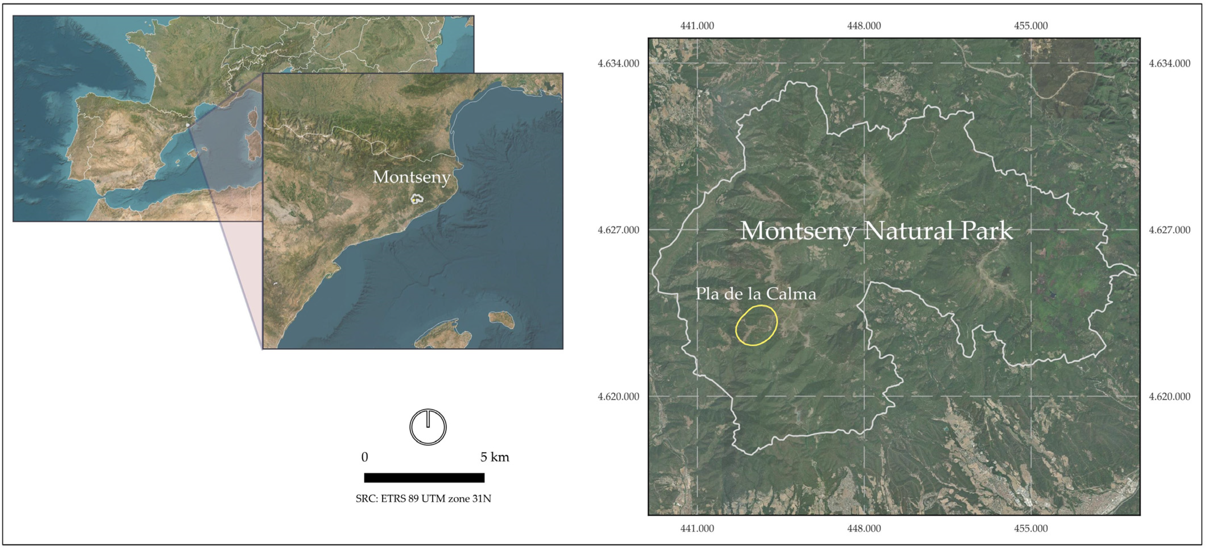
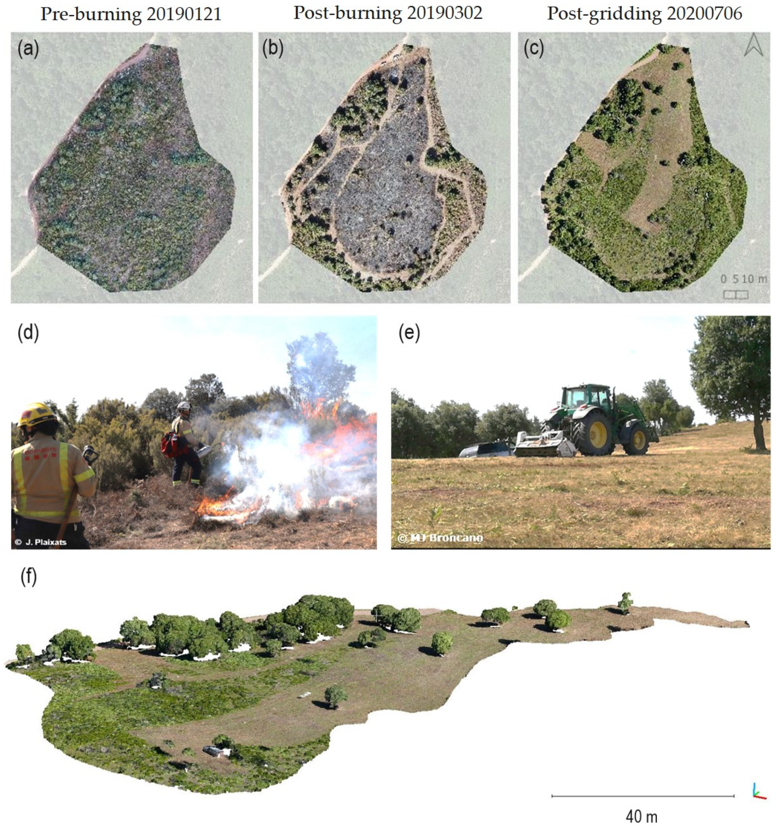
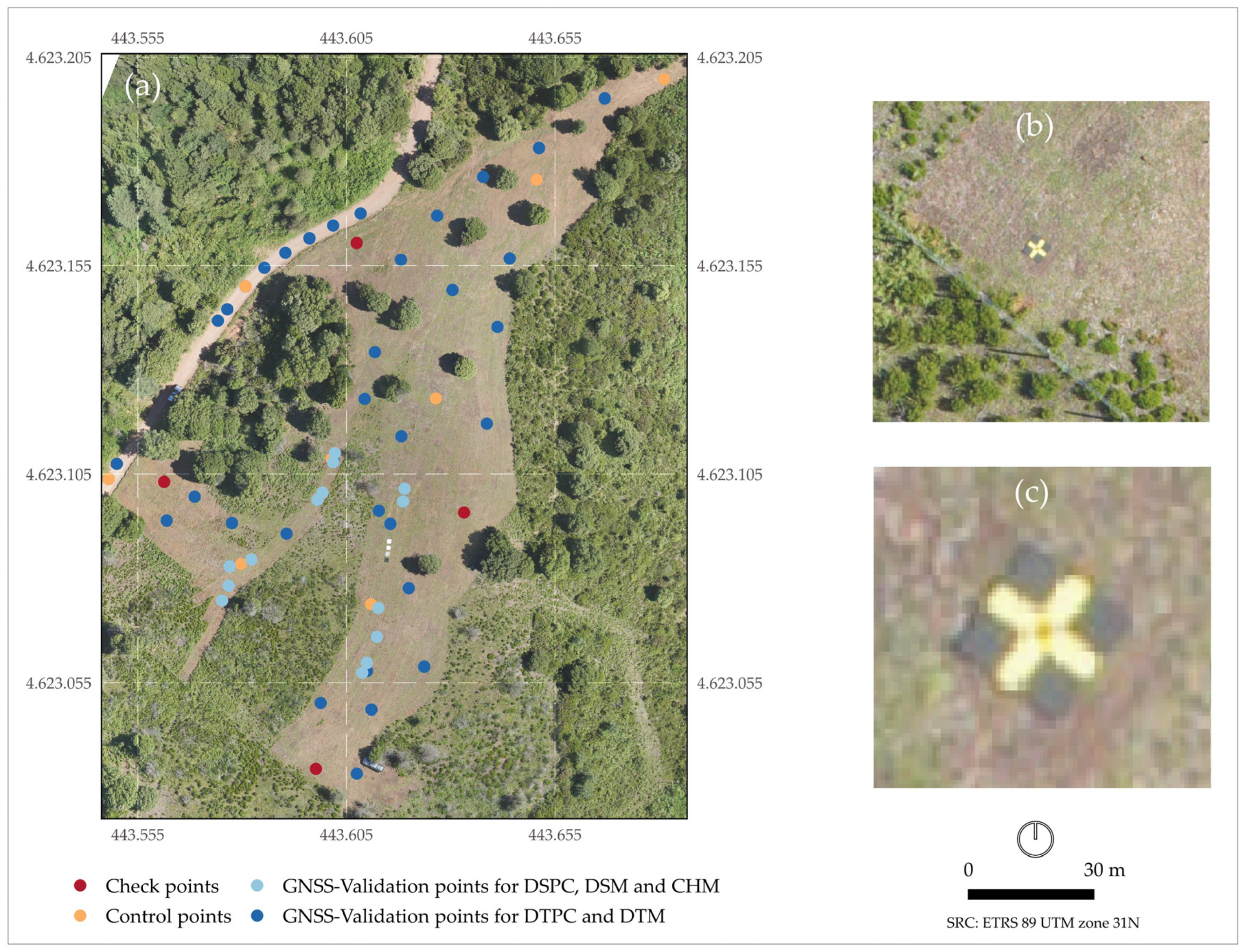
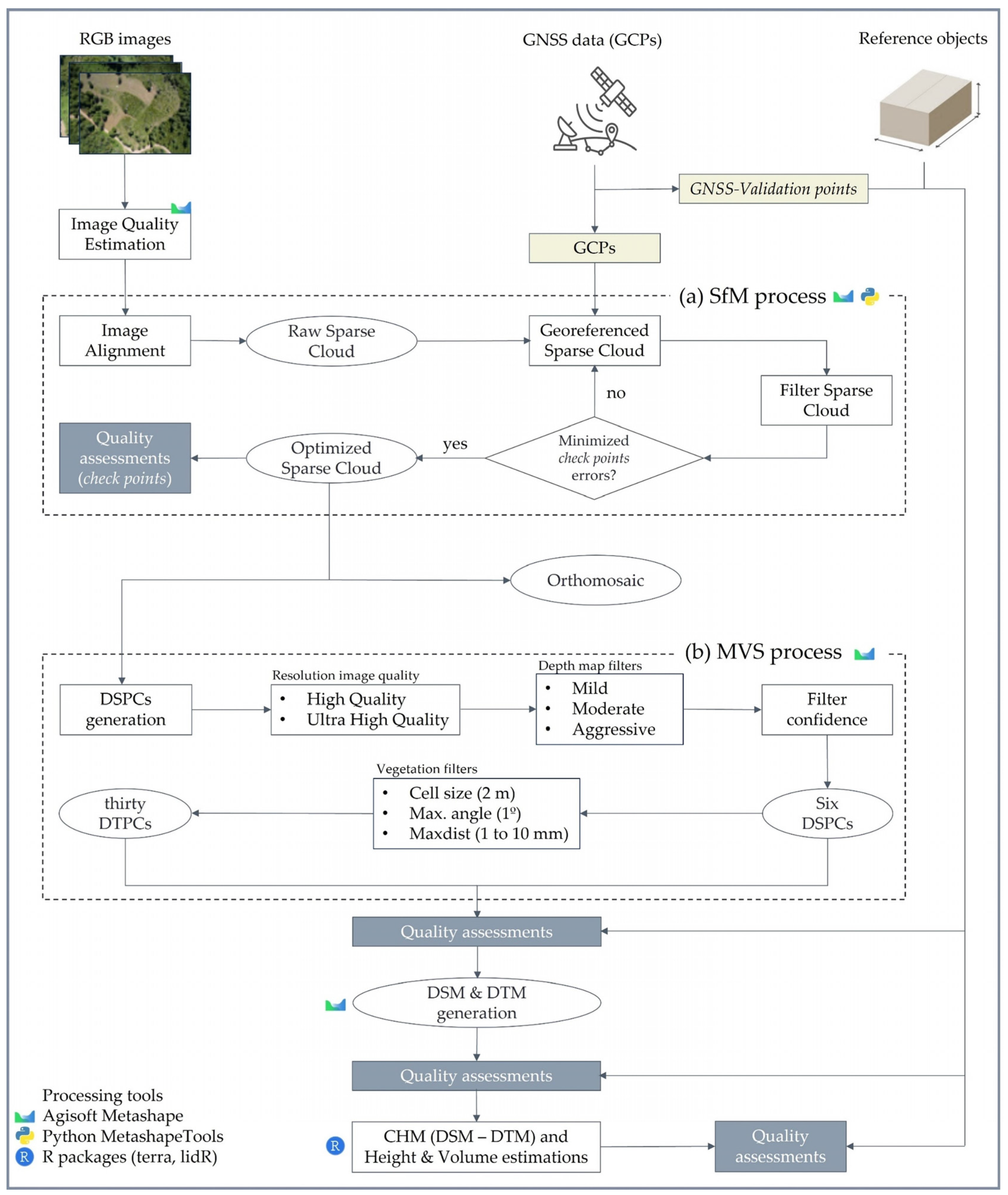
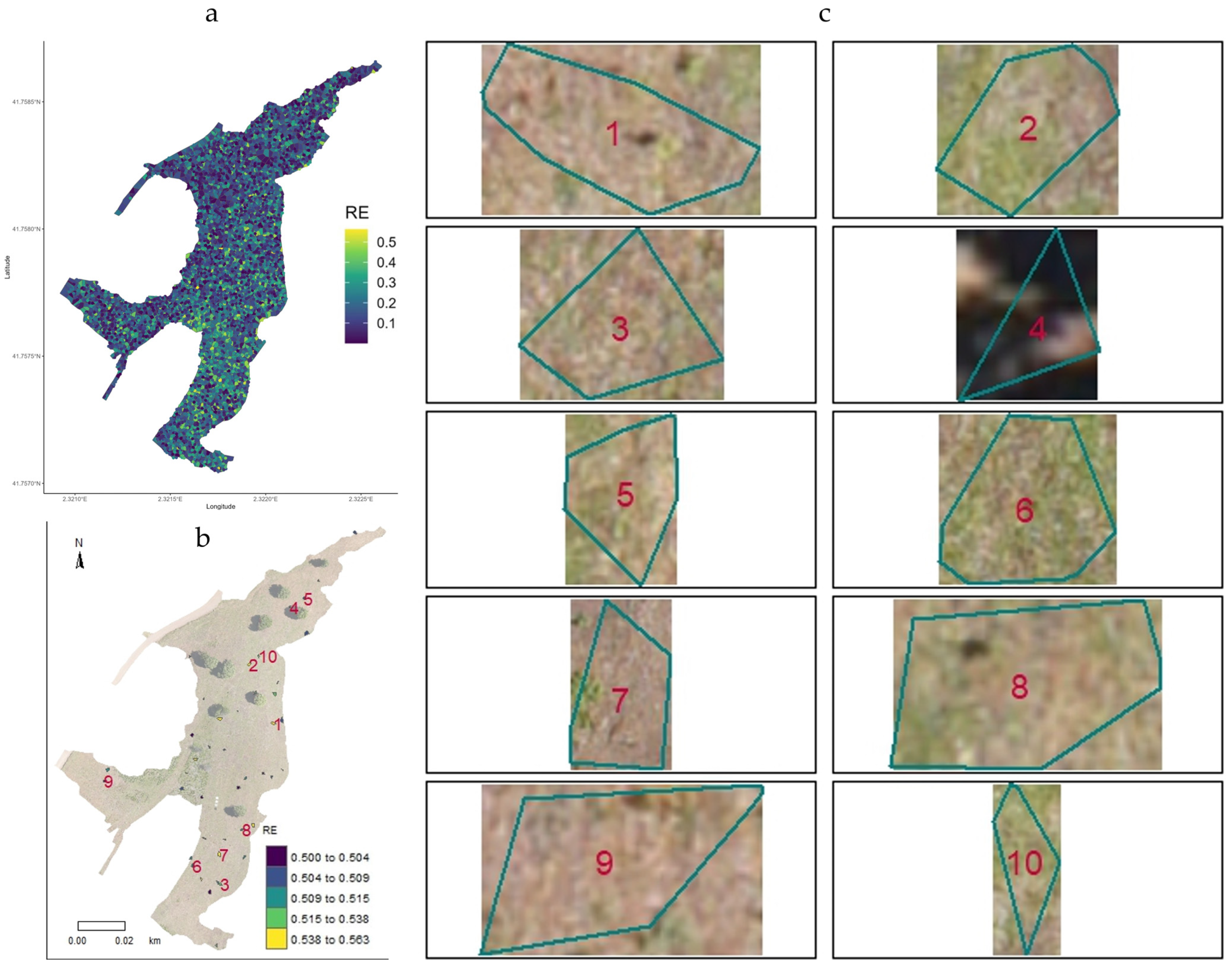
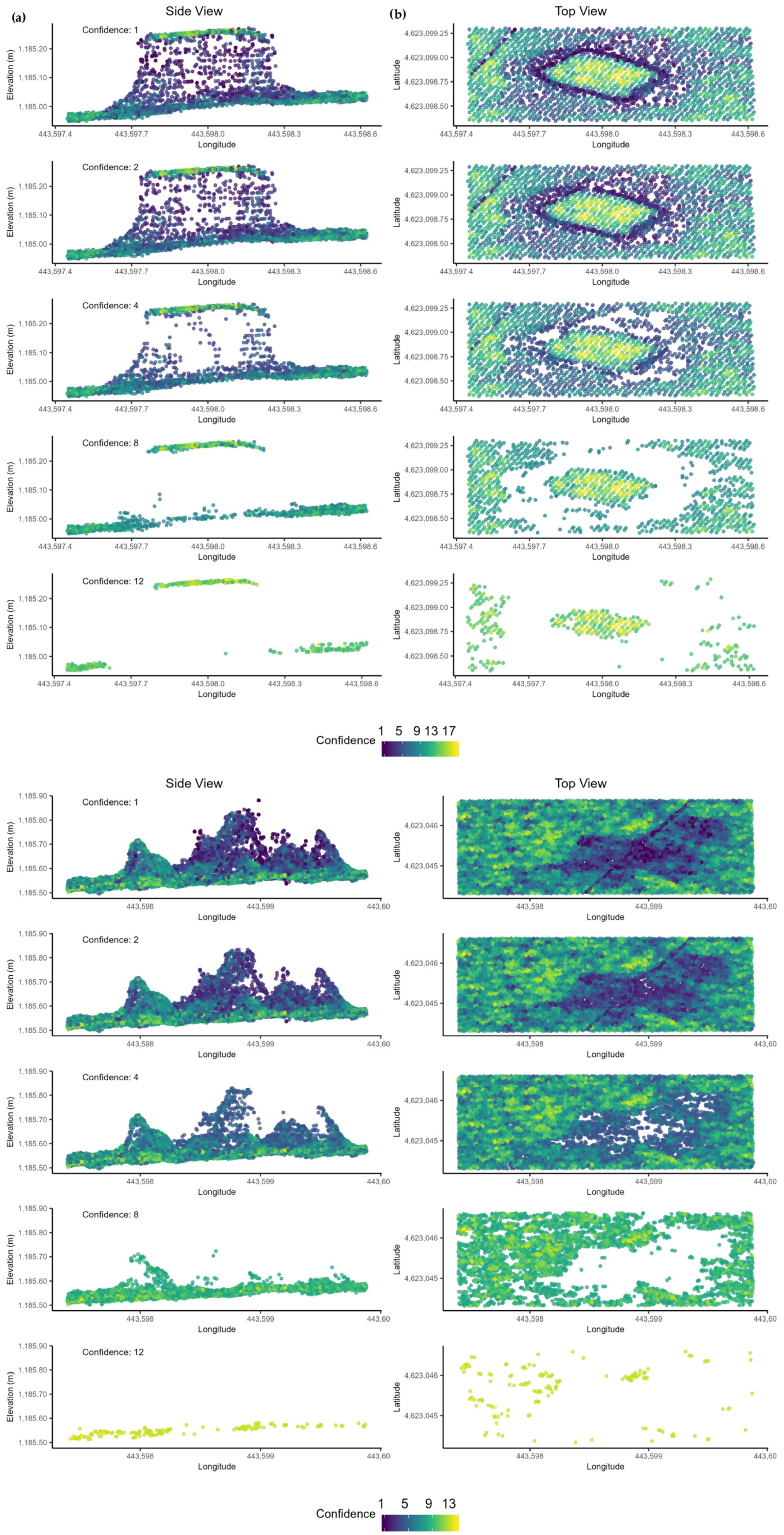
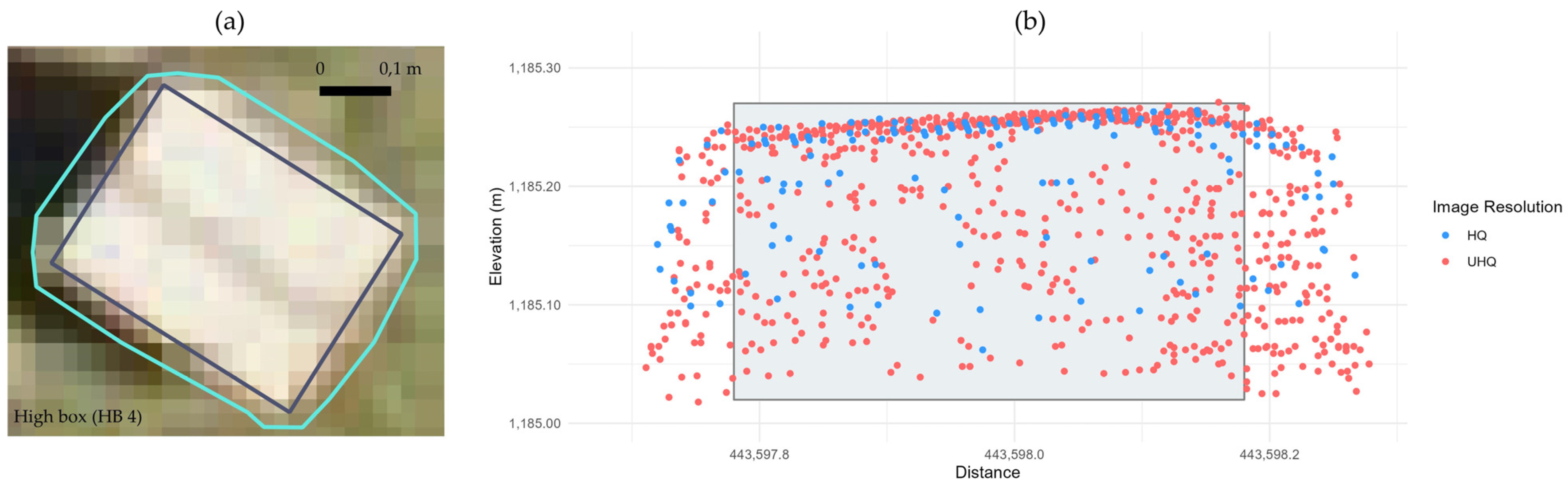
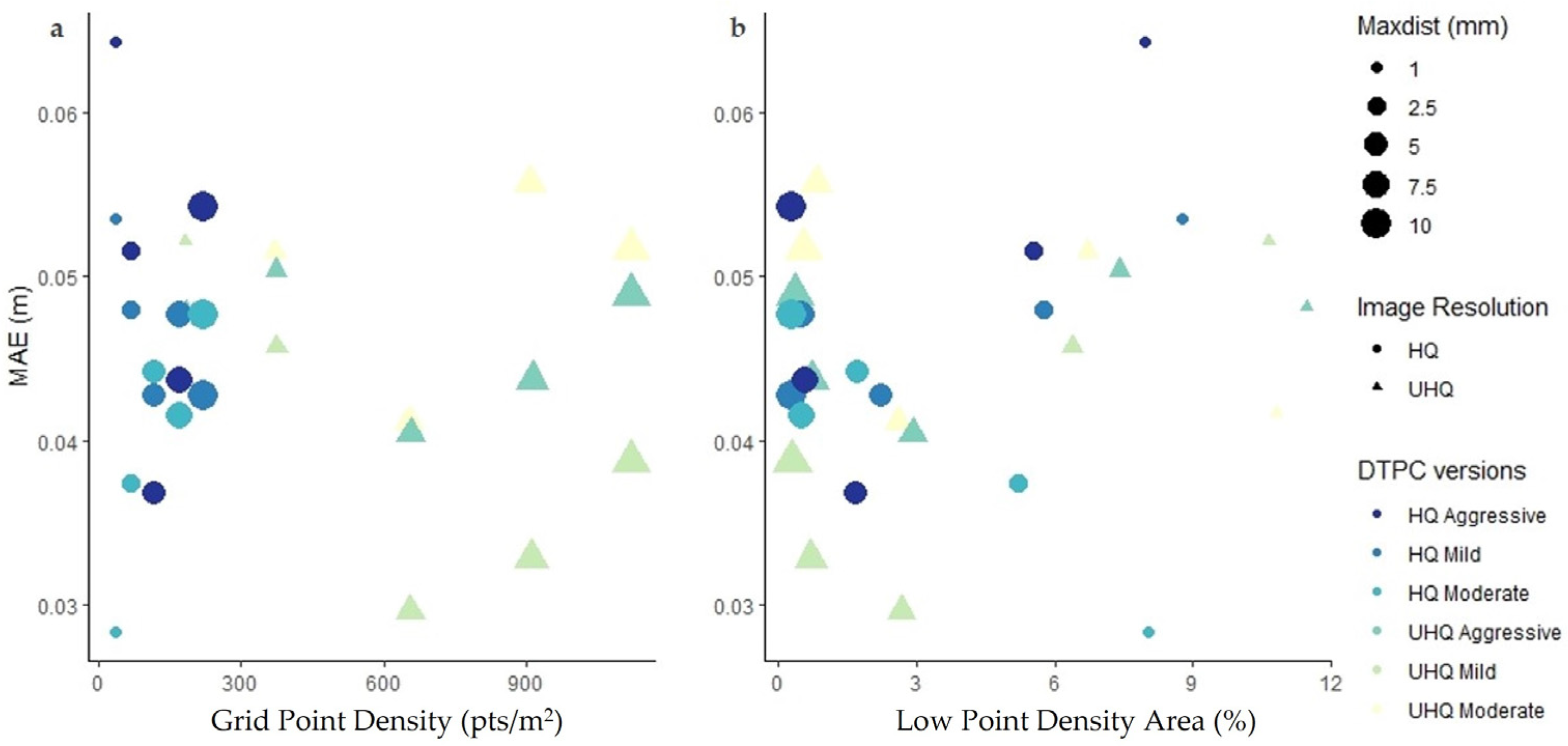
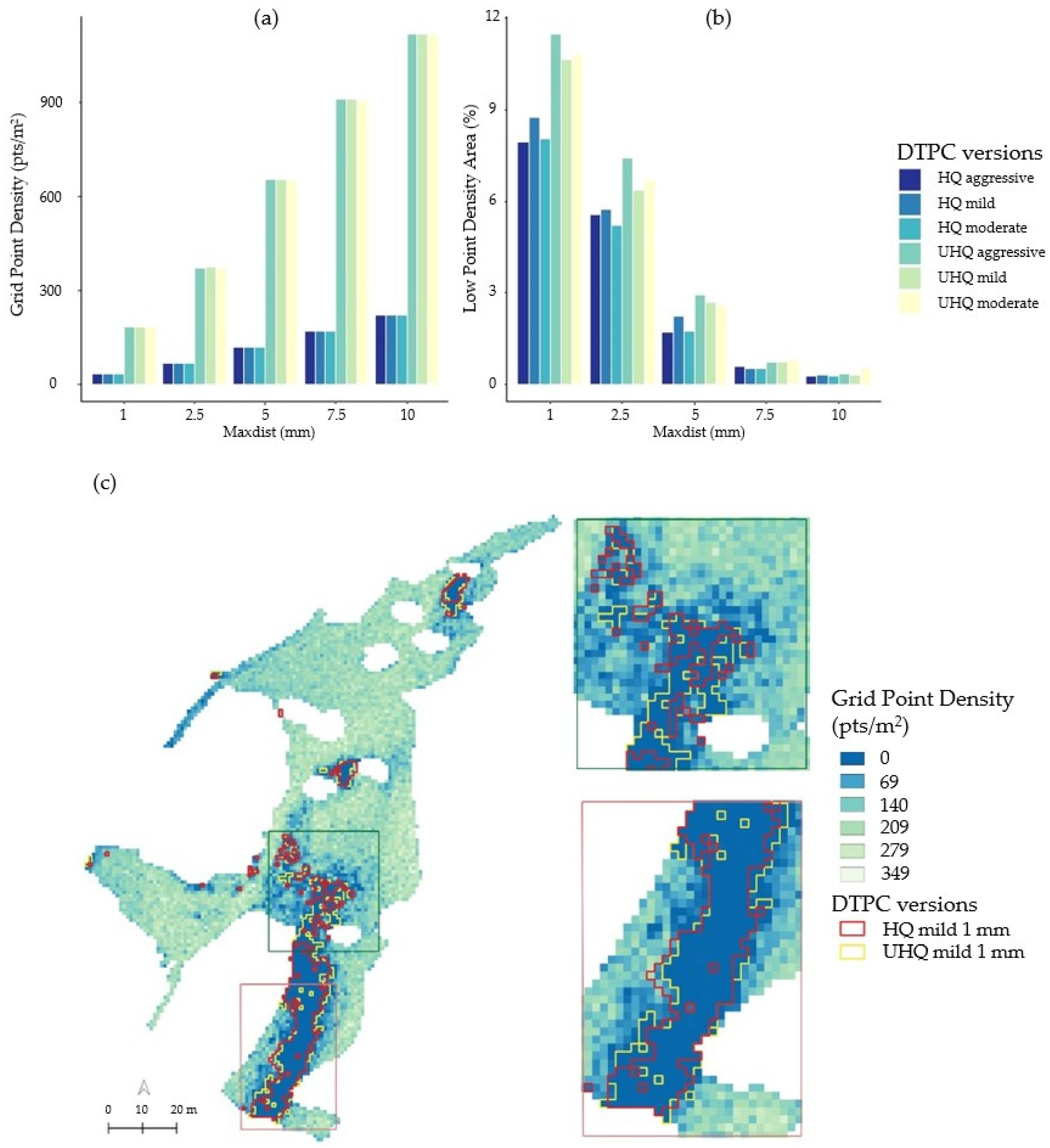
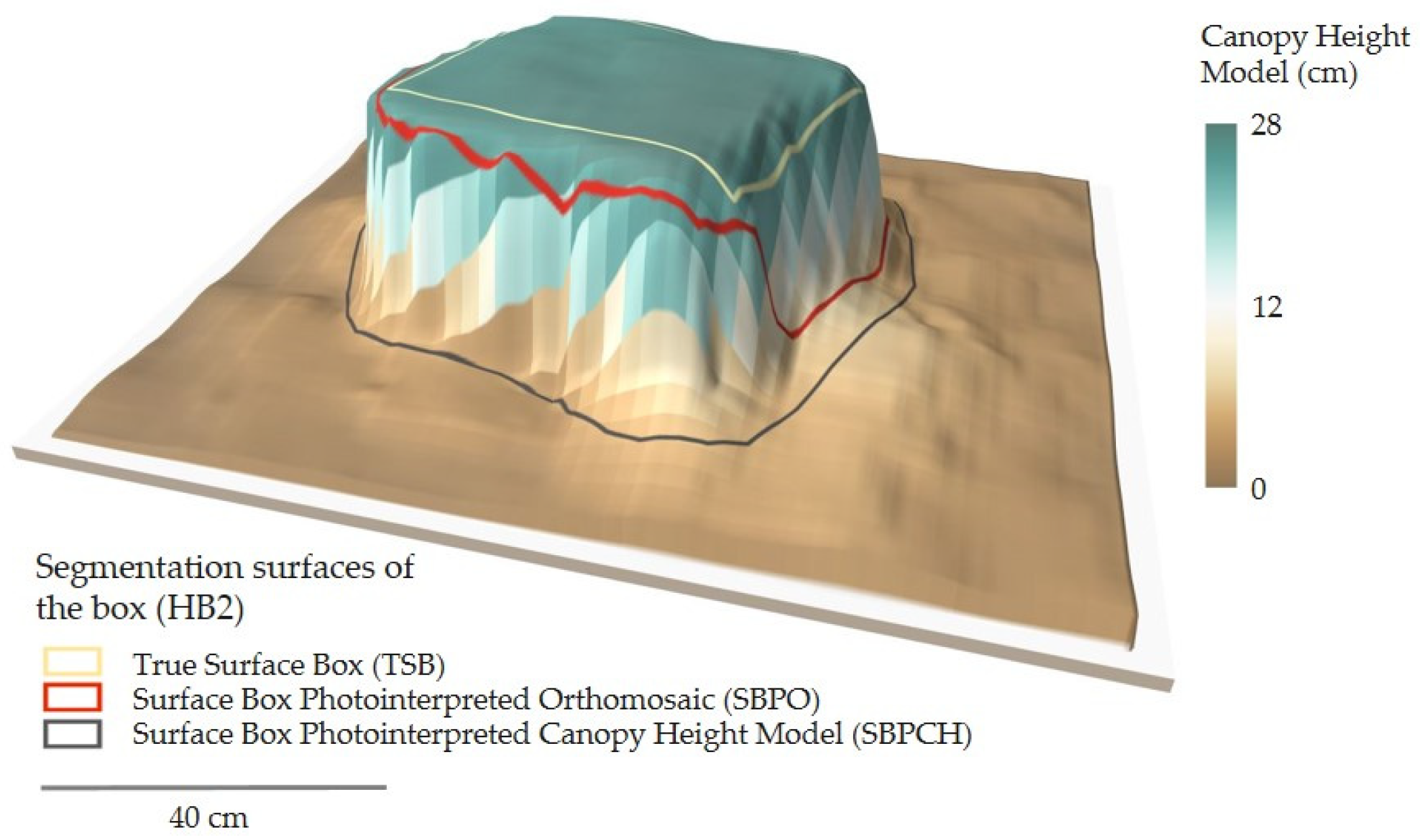
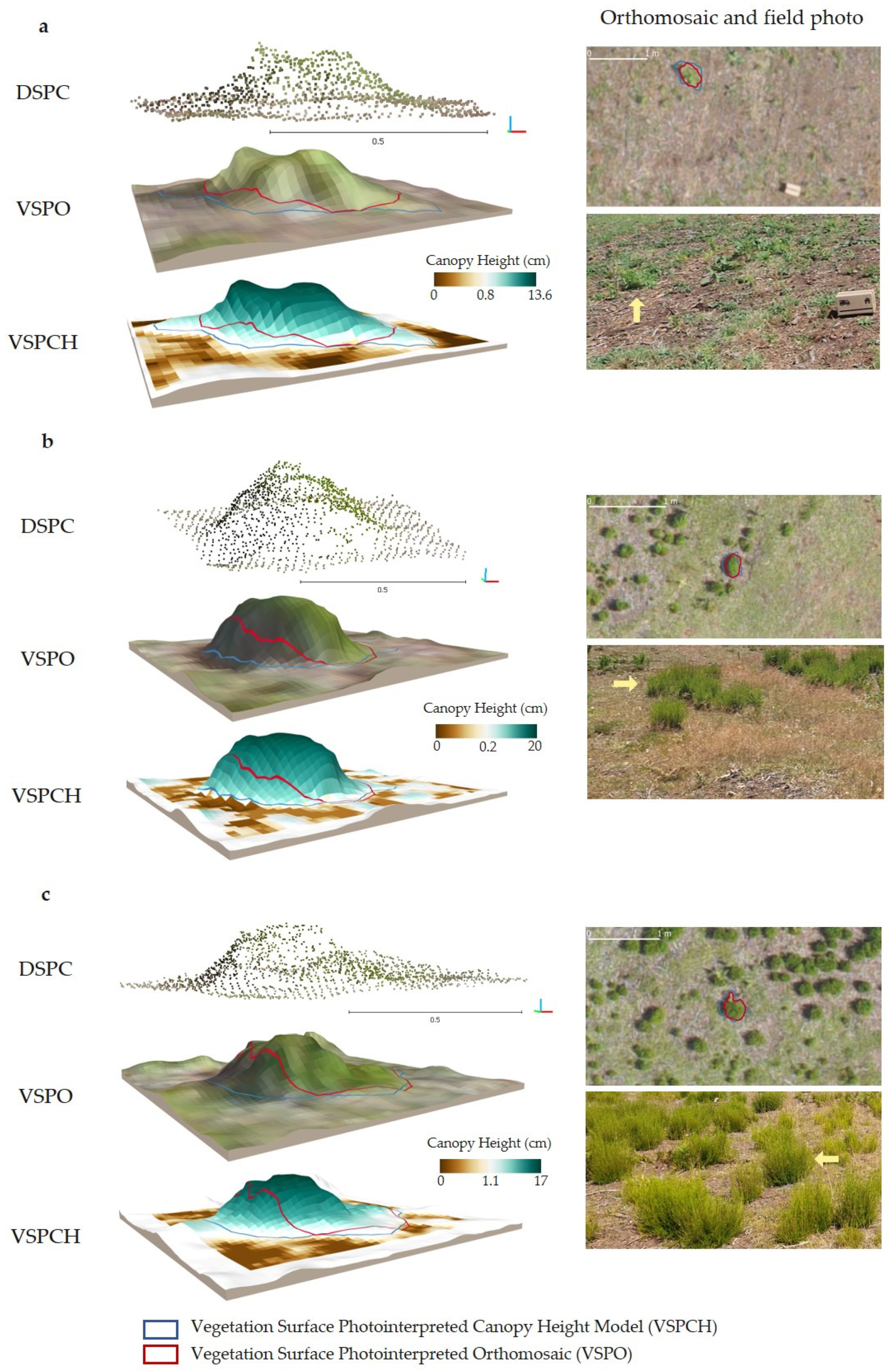
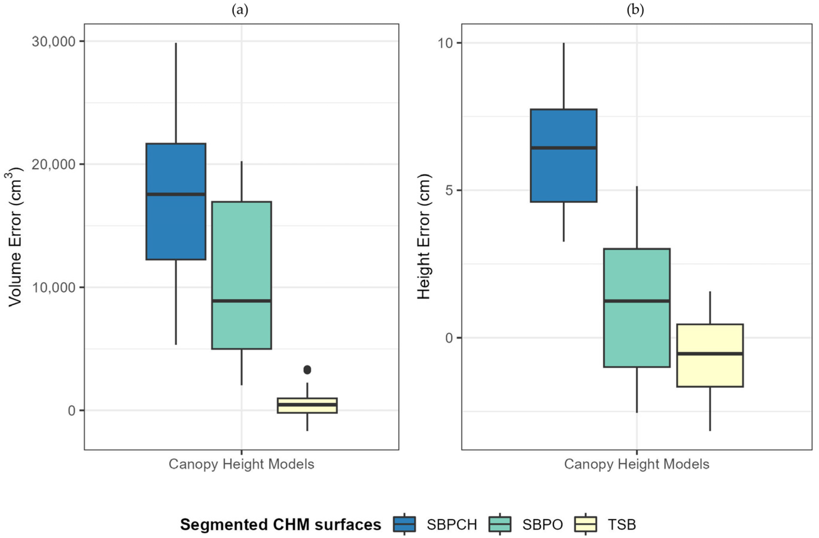
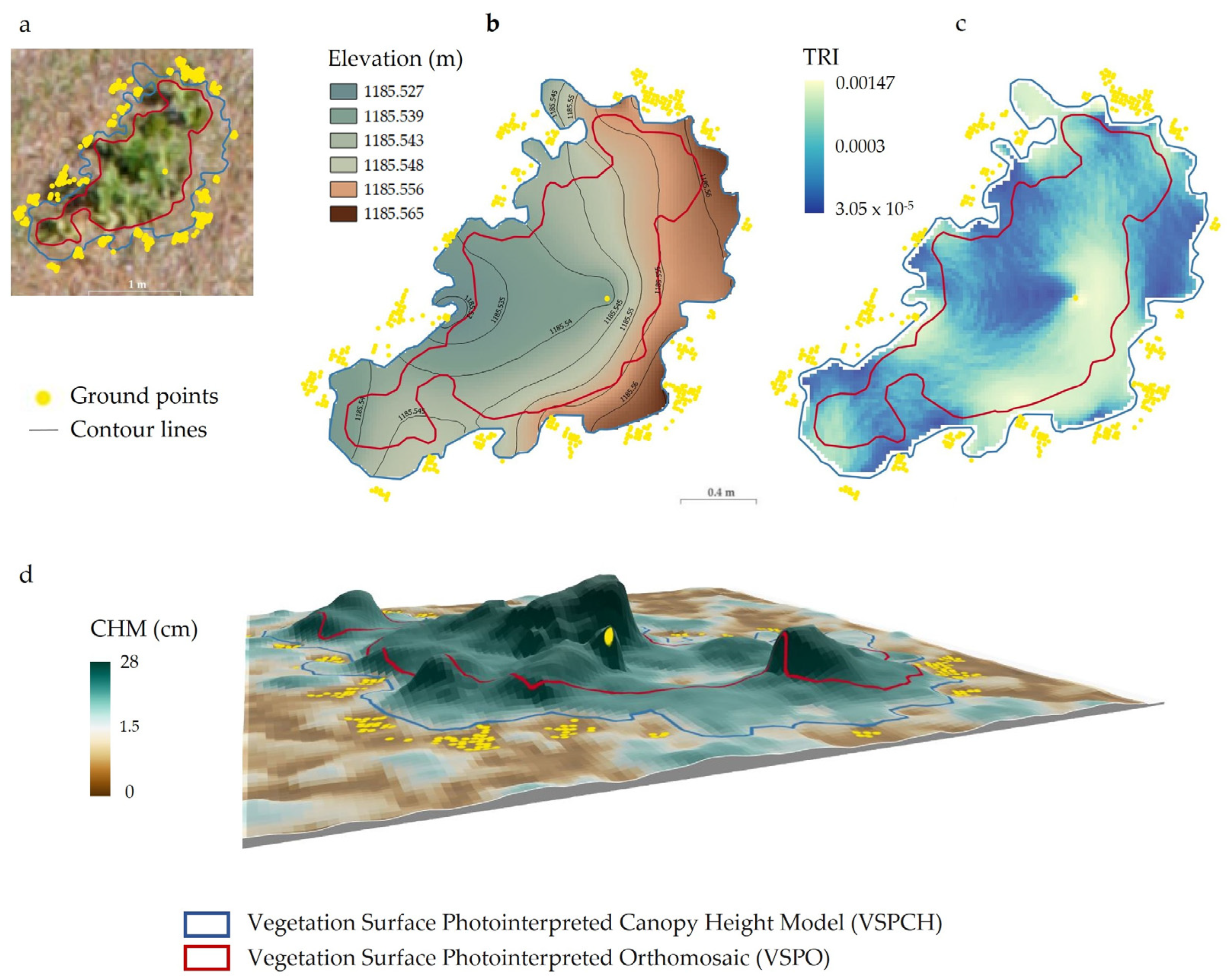
Table 1.
Description of the dimensions and heights of the boxes as reference objects.
| Reference Object | Height (cm) | Dimensions (cm) | Volume (cm3) | Upper Side Area (cm2) | No. of Boxes |
|---|---|---|---|---|---|
| Low box | 15 | 20 × 30 × 15 | 0.009 | 600 | 7 |
| High box | 25 | 30 × 40 × 25 | 0.03 | 1200 | 6 |
| Extra-high box | 30 | 25 × 40 × 30 | 0.03 | 1000 | 1 |
Table 2.
Summary of SfM results: raw vs. optimized sparse cloud. (Note: The raw sparse cloud represents the georeferenced sparse cloud, unfiltered, and excluding duplicated images. The iterative filtering process is integrated into the optimized sparse cloud. This table includes errors of control points and check points for both non-optimized and optimized sparse clouds. It also features the Root Mean Square Error (RMSE) of the linear model between Ground Control Points’ (GCPs) elevation values and predicted elevation values in both raw and optimized sparse clouds.).
| Metrics | Raw Sparse Cloud | Optimized Sparse Cloud |
|---|---|---|
| Photograms (no.) | 24 | 24 |
| Tie points (no.) | 31,379 | 29,545 |
| RMS RE (px.) | 1.239 | 0.583 |
| RMSE control points xy (m) | 0.586 | 0.016 |
| RMSE control points z (m) | 4.242 | 0.004 |
| RMSE control points xyz (m) | 4.282 | 0.017 |
| RMSE check points xy (m) | 0.530 | 0.113 |
| RMSE check points z (m) | 4.351 | 0.076 |
| RMSE check points xyz (m) | 4.383 | 0.137 |
| Elevation RMSE (m) | 4.27 | 0.12 |
Table 3.
Overview of Dense Surface Point Cloud (DSPC) characteristics based on image quality resolution (ultrahigh quality (UHQ) and high quality (HQ)) and depth filtering levels (mild, moderate, and aggressive).
Table 3.
Overview of Dense Surface Point Cloud (DSPC) characteristics based on image quality resolution (ultrahigh quality (UHQ) and high quality (HQ)) and depth filtering levels (mild, moderate, and aggressive).
| Image Quality Resolution | UHQ | HQ | ||||
|---|---|---|---|---|---|---|
| Depth Filter | Mild | Moderate | Aggressive | Mild | Moderate | Aggressive |
| Process time depth filter | 9 h 50 m | 9 h 44 m | 9 h 49 m | 2 h 48 m | 2 h 48 m | 2 h 49 m |
| Process time DSPC | 15 m 15 s | 14 m 36 s | 14 m 49 s | 3 m 48 s | 3 m 38 s | 3 m 41 s |
| No. points in DSPC raw | 15,122,249 | 15,033,502 | 14,966,021 | 3,725,108 | 3,707,369 | 3,694,205 |
| Var. in raw DSPC | 100% | −0.59% | −1.03% | −75.37% | −75.48% | −75.57% |
| No. of filtered points (confidence < 1) | 738,503 | 683,233 | 656,298 | 112,430 | 103,486 | 103,077 |
| No. points in filtered DSPC | 14,383,746 | 14,350,269 | 14,309,723 | 3,612,678 | 3,603,883 | 3,591,128 |
Table 4.
Overview of elevation accuracy and point density in 6 Dense Surface Point Cloud (DSPC) versions. These versions were generated based on varying image quality resolution (ultrahigh quality (UHQ) and high quality (HQ)) and depth filter levels (mild, moderate, and aggressive). The table includes R2 values, Mean Absolute Error (MAE) from regression models comparing GNSS validation point elevation values to predicted elevations on 14 reference boxes, Standard Deviation, and point density metrics.
| Image Quality Resolution | Depth Filter | R2 | Elevation MAE (m) | SD (m) | Density (pts/m2) |
|---|---|---|---|---|---|
| Mild | 0.9914 | 0.056 | 0.007 | 2022.81 | |
| UHQ | Moderate | 0.9907 | 0.059 | 0.005 | 2010.56 |
| Aggressive | 0.9911 | 0.059 | 0.006 | 2011.95 | |
| Mild | 0.9904 | 0.055 | 0.006 | 530.65 | |
| HQ | Moderate | 0.9909 | 0.056 | 0.007 | 544.17 |
| Aggressive | 0.9906 | 0.056 | 0.006 | 548.11 |
Table 5.
Analysis of variance (one-way ANOVA) for elevation and point density of reference objects across different image quality resolution levels (UHQ and HQ) and depth filters (mild, moderate, and aggressive) for the 6 DSPC versions. Note: * denotes p < 0.05; ** denotes p < 0.01; *** denotes p < 0.001.
| Filters Parameters | Elevation Error (m) | Density (pts/m2) | ||
|---|---|---|---|---|
| F | p-Value | F | p-Value | |
| Image quality resolution | 0.042 | 0.838 | 5902 | <2 × 10⁻¹ 6 *** |
| Image quality resolution and depth filter | 0.009 | 1 | 1120 | <2 × 10⁻¹ 6 *** |
Table 6.
Analysis of the elevation accuracy of selected DSMs and DTMs, including the estimated R2 of the linear regression between observed GNSS validation points elevation values and predicted DSM and DTM elevation values and standard linear regression metrics such as MAE.
Table 6.
Analysis of the elevation accuracy of selected DSMs and DTMs, including the estimated R2 of the linear regression between observed GNSS validation points elevation values and predicted DSM and DTM elevation values and standard linear regression metrics such as MAE.
| DEMs | Image Quality Resolution | Depth Filter | Maxdist (mm) | Number of Samples | R2 | Elevation MAE (m) |
|---|---|---|---|---|---|---|
| DSM | UHQ | Mild | - | 12 | 0.9912 | 0.057 |
| DTM | UHQ | Mild | 5 | 45 | 0.9992 | 0.048 |
Table 7.
Summary of height and volume measurement MAE accuracy estimated over the reference boxes and derived from the Canopy Height Model versions (true surface box (TSB), surface box photointerpreted orthomosaic (SBPO), and surface box photointerpreted canopy height (SBPCH).
Table 7.
Summary of height and volume measurement MAE accuracy estimated over the reference boxes and derived from the Canopy Height Model versions (true surface box (TSB), surface box photointerpreted orthomosaic (SBPO), and surface box photointerpreted canopy height (SBPCH).
| CHM Versions | Height MAE (cm) | Volume MAE (cm3) |
|---|---|---|
| True surface box (TSB) | 1.20 | 909.30 |
| Surface box photointerpreted orthomosaic (SBPO) | 1.88 | 8899.41 |
| Surface box photointerpreted canopy height (SBPCH) | 6.43 | 17,552.44 |
Disclaimer/Publisher’s Note: The statements, opinions and data contained in all publications are solely those of the individual author(s) and contributor(s) and not of MDPI and/or the editor(s). MDPI and/or the editor(s) disclaim responsibility for any injury to people or property resulting from any ideas, methods, instructions or products referred to in the content. |
© 2023 by the authors. Licensee MDPI, Basel, Switzerland. This article is an open access article distributed under the terms and conditions of the Creative Commons Attribution (CC BY) license (https://creativecommons.org/licenses/by/4.0/).
Share and Cite
MDPI and ACS Style
Mestre-Runge, C.; Ludwig, M.; Sebastià, M.T.; Plaixats, J.; Lobo, A. Optimizing Drone-Based Surface Models for Prescribed Fire Monitoring. Fire 2023, 6, 419. https://doi.org/10.3390/fire6110419
AMA Style
Mestre-Runge C, Ludwig M, Sebastià MT, Plaixats J, Lobo A. Optimizing Drone-Based Surface Models for Prescribed Fire Monitoring. Fire. 2023; 6(11):419. https://doi.org/10.3390/fire6110419
Chicago/Turabian StyleMestre-Runge, Christian, Marvin Ludwig, Maria Teresa Sebastià, Josefina Plaixats, and Agustin Lobo. 2023. "Optimizing Drone-Based Surface Models for Prescribed Fire Monitoring" Fire 6, no. 11: 419. https://doi.org/10.3390/fire6110419