
A New Fire Danger Index Developed by Random Forest Analysis of Remote Sensing Derived Fire Sizes

1
Fenner School of Environment & Society, College of Science, The Australian National University, Canberra, ACT 2601, Australia
2
School of Engineering, College of Engineering and Computer Science, The Australian National University, Canberra, ACT 2601, Australia
*
Author to whom correspondence should be addressed.
Fire 2022, 5(5), 152; https://doi.org/10.3390/fire5050152
Submission received: 20 August 2022
/
Revised: 14 September 2022
/
Accepted: 19 September 2022
/
Published: 29 September 2022
(This article belongs to the Section Fire Science Models, Remote Sensing, and Data)
Abstract
:Studies using remote sensing data for fire danger prediction have primarily relied on fire ignitions data to develop fire danger indices (FDIs). However, these data may only represent conditions suitable for ignition but may not represent fire danger conditions causing escalating fire size. The fire-related response variable’s scalability is a key factor that forms a basis for an FDI to include a broader range of fire danger conditions. Remote sensing derived fire size is a scalable fire characteristic encapsulating all possible fire sizes that previously occurred in the landscape, including extreme fire events. Consequently, we propose a new FDI that uses remote sensing derived fire size as a response variable. We computed fire sizes from the Moderate Resolution Imaging Spectroradiometer (MODIS) satellite instrument burned area. We applied random forest (RF) and logistic regression (LR) to develop the FDI for Australia. RF models performed better than LR, and the higher predicted probabilities demonstrated higher chances for ignited fires to be escalated to larger fire sizes at a regional scale across Australia. However, the predicted probabilities cannot be related to the specific range of fire sizes due to data limitations. Further research with higher temporal and spatial resolution data of both the response and predictor variables can help establish a better relationship between a specific range of fire sizes and the predicted probabilities.
1. Introduction
Bushfires can cause substantial economic, environmental, and human losses [1]. In recent decades, the extreme bushfires at the urban interfaces of the major cities in Australia have burnt millions of hectares of land [2]. The bushfires of 2019–2020 burned an unprecedented 5.67 Mn Ha of forested area across Australia and destroyed around 2500 houses [3,4]. These losses could be minimized or avoided with an accurate forewarning like other natural disasters. Bushfire danger prediction models are vital in timely forewarning about fire events, especially extreme ones [1]. Australia’s current operational fire danger prediction system relies on McArthur fire danger indices (FDIs). It has shown many limitations, such as non-verification and under-prediction of fire danger highlighted by various studies, including missing extreme fire events [5,6,7]. With the forecasted increase in the frequency of extreme bushfires in the future [1,8], there is a strong focus on the trial and development of new FDIs for Australia using more contemporary science, including the development of the new Australian Fire Danger Rating System which is under trial and will be deployed in near future [7,9,10].
Fire danger modeling is developed for different fire-related characteristics [11,12]. For example, the spread component in operational fire models is quantified using the rate of fire spread and the energy release (fire intensity component), with the fire-line intensity or heat available to the fire per square foot [12,13]. Operational fire danger models then calibrate these components with the difficulty of suppression or fire containment efforts [11,13]. Thus, the fire danger modeling relies on the response variable characteristics (rate of spread or fireline intensity) to predict fire danger [7,9]. Two essential characteristics for a response variable to be valid for an FDI are: (1) its scalability to present bushfire danger conditions from low to extreme and beyond and; (2) its feasibility to be easily verifiable [6,7]. The USA. National Fire Danger Rating System, the Canadian Fire Weather Index (FWI), and the Australian McArthur Fire Danger Ratings System achieved scalability by relating all possible ranges of the rate of fire spread and fire-line intensity (response variables) to predictors through empirical and quasi-empirical fire behavior processes [11,12,14,15]. The ratings were scaled from Low to Extreme fire danger classes based on the observed ranges of the response variable [12,16]. The second quality of verifiability depends on how easily FDIs can be measured. This quality helps post-event verification, contributing to further improvement of FDI [7]. The McArthur FDIs currently used for operational fire management in Australia are constrained because measurement of fire spread rate is challenging, limiting the further improvement of the McArthur FDIs [5,7]. Although using newer technologies such as line scans during wildfire events can help overcome these limitations, these airborne missions are costly [17].
Remote sensing derived information on fire characteristics offers opportunities to fulfill these two essential characteristics of an FDI. The physical fire characteristics such as fire sizes, fire radiative power (FRP), and brightness temperature are available at various temporal and spatial scales, which offers a key advantage over the experimentally derived variables such as the rate of spread or the fire-line intensity [18,19,20]. These fire characteristics are scalable from low to maximum possible values and easily verifiable because of their continuous temporal and spatial availability. Thus, these remote sensing fire characteristics provide a basis to develop robust FDIs with convenient post-event verification and the opportunity to improve FDIs further.
Recently, several FDI models have incorporated various remote sensing derived fire characteristics, including fire ignitions [21,22], fire density [23], remote sensing brightness temperature [8], and burned area [24]. The fire ignitions were primarily used as a response variable for presenting a maximum fire danger [25,26]. However, fire ignition or ignition density may only represent conditions affecting the likelihood of fires starting and may not necessarily represent the predictor conditions responsible for escalating small fires to larger events. For example, an ignited fire area would be higher under elevated wind speed than lower wind speed, given all other predictors are held constant. On the other hand, studies using the burned area as a response variable considered fire sizes with a specific threshold to separate small and large fires. For example, Preisler, Burgan, Eidenshink, Klaver and Klaver [24] predicted large fires on federal land, in the USA, and used a threshold of 40.47 Ha to differentiate between small and large fires. Similarly, Cortez and Morais [27] predicted burned areas for small fires (most fires less than 50 Ha) in Montesinho Natural Park, Portugal. Bradstock, et al. [28] predicted large fires in the greater Sydney region, South-East Australia, using a threshold of 1000 Ha for large fires. Whereas in Australia, fires much larger than 1000 Ha frequently occur with a median and 75th quartile fire size of 2500 and 12,500 Ha, respectively [29]. Thus, a full range of fire sizes previously occurred in the Australian landscape could be a suitable response variable presenting the full range of fire danger conditions driving varying fire sizes across the Australian landscape. Furthermore, extreme fire weather conditions are the main drivers of large fires, suggesting fire size as a suitable response variable [6,30,31,32].
Machine learning algorithms are powerful predictive tools and have been frequently used to predict fire danger probabilities, including being trained and evaluated with fire ignition (location only) [33,34] and fires per area (fire density) [23,25]. The performance of the algorithms is considered good if most fires, from the evaluation data, fall in higher predicted probabilities [22,26]. However, these methods could be made more meaningful if trained on a full range of fire sizes instead of fire ignition or density. For example, algorithms trained with a full range of fire sizes could predict probabilities of the fire sizes in addition to ignitions and density. Consequently, the fire sizes would be a more meaningful metric for the machine learning algorithms to learn from the variability of a broader range of fire danger conditions across the Australian landscape. Thus, the algorithms trained with a fire size variable could better predict the fires and their chances of growing to larger fire sizes.
We used remote sensing derived fire sizes to develop a novel FDI for continental Australia using random forest and logistic regression models. The study hypothesized that machine learning algorithms, trained with a full range of fire sizes, could predict the probabilities for fires that have the potential to spread to large fire sizes with reasonable accuracy.
2. Materials and Methods
2.1. Data
We computed fire sizes (response variable) from the MODIS burned area product MCD64A1 on a weekly scale. We used a weekly time scale so that all burned pixels in a patch adjacent to at least one other pixel from any side, could be joined, creating a continuous patch of burned pixels. MCD64A1 (burned area) is computed by applying dynamic thresholds to the burn-sensitive vegetation index generated from the 500-m Terra (“MOD09GH”) and Aqua (“MYD09GH”) surface reflectance products [35]. The MODIS active fire products guide the accuracy of the burned pixels, and MODIS landcover products refine the accuracy of the burned pixels by accounting for differences in the pre and post-burn surface reflectance across different vegetation types [20,36,37]. MCD64A1 is released monthly with a spatial resolution of 500 m × 500 m and labels each burned pixel with the ordinal day of the year on which that pixel was burned [36]. It is available from the Land Processes Distributed Active Archive Centre (LPDAAC).
We used ten predictors based on their known role in fire danger modeling. The predictors included: temperature (°C), vapor pressure (hpa), rainfall (mm), wind speed (kmh−1), relative humidity (%), drought factor (DF) (dimensionless), soil moisture deficit (mm) (SMD), forest fire danger index (dimensionless) (FFDI), live fuel moisture content (LFMC) (%), and soil moisture content (%) derived from the Australian Water Resource Assessment—Landscape Model (AWRA-L). We sourced temperature, vapor pressure, and rainfall data from the Terrestrial Ecosystem Research Network Discovery portal. This data was developed by Jones, et al. [37], as one of the components of the Australian Water Availability Project (AWAP), by applying topography resolving analysis to in-situ observations [38]. It has a spatial resolution of 0.05° and is available at monthly and daily temporal resolutions. We used 24-h daily maximum temperature and total rainfall from 09:00 am to 09:00 am the next day, and the 03:00 pm vapor pressure data represents afternoon drier conditions. We computed the daily wind speed data by averaging the 10 m Eastward (u-component) and 10 m Northward (v-component) hourly components of the ERA- 5 wind speed data [39]. ERA-5 is a reanalysis data project by the European Center for Medium-Range Weather Forecasts (ECMWF). ERA-5 data can be accessed from Copernicus Climate Change Service (C3S), providing hourly estimates of various meteorological factors [39].
We computed relative humidity from the AWAP temperature and vapor pressure data following Nolan, et al. [40]. Drought factor (DF) and soil moisture deficit (SMD) represent the dryness of the fuel layers on the forest floor and soil moisture deficit, respectively [41]. We calculated the DF and SMD using the AWAP rainfall and temperature data following Finkele, et al. [42] and using Keetch and Byram drought Index (KBDI) approach [43]. FFDI is commonly used in Australia for fire danger prediction and computed following Noble, et al. [44] and Dowdy [45]. We included FFDI as a predictor because FFDI is directly related to the rate of fire spread across Australia [46]. This relationship means that the highest FFDI values would be expected to result in larger fire sizes, and vice versa. Thus, we expected that the FFDI values would help the model to better learn the relationship between predictors and fire sizes. Thus, better performing in predicting fire size probabilities. Moreover, the predictor’s importance property of RF allowed exploring its importance relative to other predictors used in the model. Soil moisture has an established role in fire danger prediction [47]. AWRA-L root zone soil moisture represents the percentage of soil moisture in the top one-metre layer of the soil and consists of upper (0–0.1 m, AWRA-L (s0)) and lower (0.1–0.9 m, AWRA-L (ss)) soil moisture layers [48]. AWRA-L is a water balance model that estimates soil moisture, precipitation, evapotranspiration, run-off, and deep drainage at 0.05° degree grids across Australia [49]. The LFMC represented the percentage water content relative to the dry vegetation mass and was sourced from a semi-operational product available at the Australian Flammability Monitoring System via the National Computational Infrastructure (NCI)’s Thredds server. The product is generated using the MODIS reflectance data and radiative transfer model inversion techniques [50]. LFMC has shown a reasonable relationship with fire risk across Australia and is available at 0.005° degree grids [50].
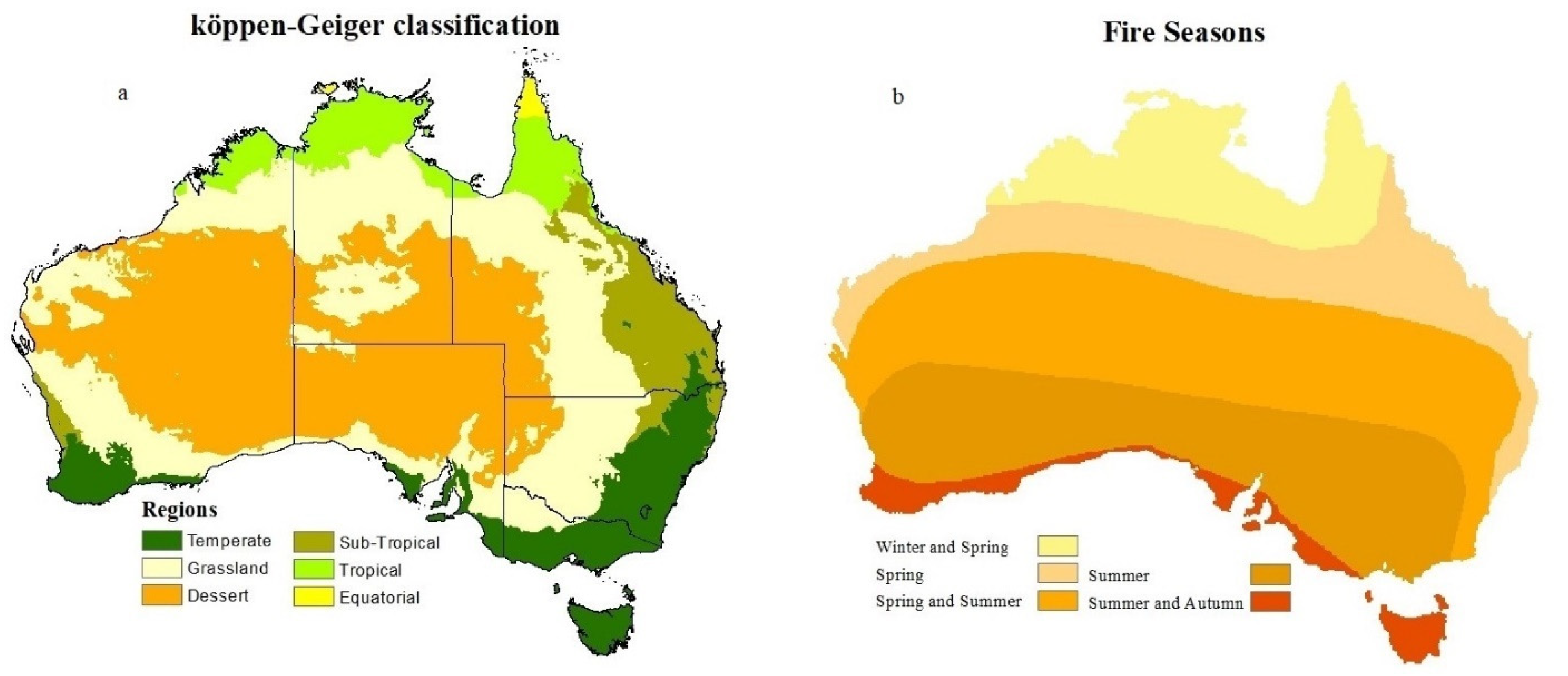
We used the Köppen-Geiger classification system to develop regional FDI models for each climate zone (Figure 1a). Köppen-Geiger classification system considers temperature and precipitation as primary drivers of vegetation types and classifies Australia into six climate zones [51]. The classification uses broadscale vegetation types to different region types [51]. Thus, a suitable re-classification is proposed to develop models for each zone based on its primary vegetation type while also considering regional differences in climatic variables.
Fire season represents conditions suitable for ignitions and fire spread [52]. In Australia, the fire season occurs at different times for different regions, from winter and spring in the north to summer and autumn in the south (Figure 1b) [53]. We only used the response and predictor variables from the fire seasons for FDI modeling. Fire seasons data avoids large-scale agricultural and hazard reduction burns conducted outside the fire seasons. Thus, including data from outside the fire seasons could result in large fire size samples under relatively milder conditions, causing mixed messaging and potentially degrading the model’s accuracy. We sampled/processed all the other data by coding scripts in Python 3.6.
2.2. Methods
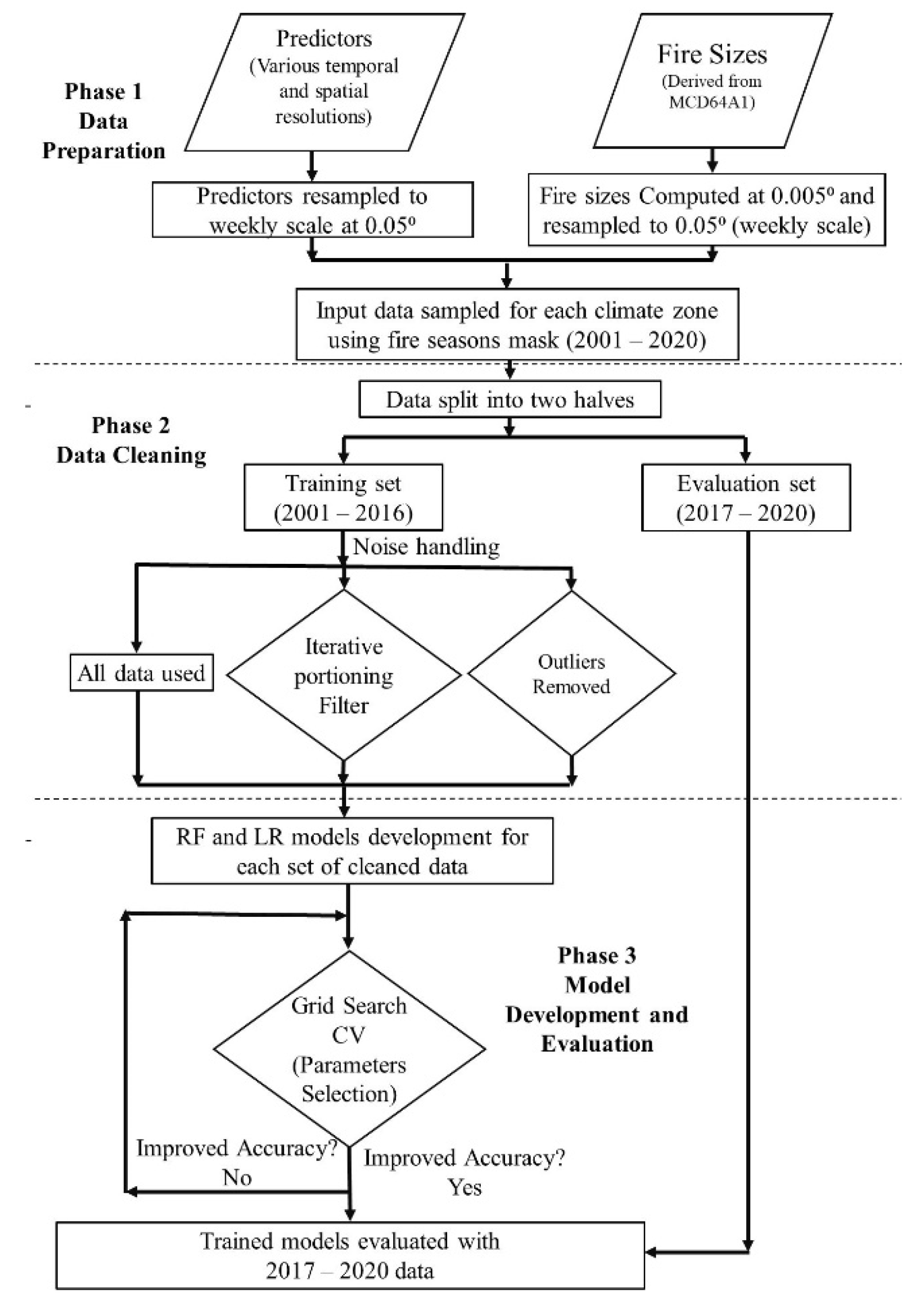
Our method consists of three distinct phases (Figure 2). Firstly, we prepared the predictors and response variables data. Secondly, we split the data into training (2001–2016) and validation sets (2017–2020). We then refined the data and generated three curated data sets, each using a different process for noise handling. Finally, in the third phase, we developed the RF and LR models for each data type and climate zone.
The predictors and response variables data were at different spatial resolutions. We resampled all data to 0.05° spatial resolution for this study because most of the predictors, including AWAP and AWRA-L datasets, were available at this resolution. Moreover, this spatial resolution allowed reasonable computational efficiency and thus convenient repeatability in fine-tuning models at a regional scale across Australia. However, spatial and temporal resolutions play an essential role in such analysis because the coarse resolution could cause averaging in some of the predictors and the response variables, thereby masking significant predictor effects on the response variable. We calculated weekly averages for the entire time series. The weekly scale avoids the locational inaccuracies associated with characterizing burned pixels at a daily scale [20]. Fire sizes (response variable) were computed from the weekly 500 m × 500 m grids and then resampled to 5 km × 5 km grids using the maximum resampling parameter. We assigned each pixel, within a fire size patch, the value equal to the total area of that particular fire patch but retained each pixel within that patch as a different data point. We used each pixel predictor data within a particular fire size. This sampling method (1) presented reasonable variability to machine learning algorithms which typically learn from variation in the predictor’s data, and (2) allowed a sufficiently large number of samples required to increase the reliability of classification accuracy for fire sizes class. The distribution of the fire size samples for each climate zone is shown in Figure 3. We used fire size (Class 1) data samples as class 1 samples and randomly sampled an equal number of no-fire (Class 0) data samples. Following previous studies, the fire and no-fire classes reflect machine learning algorithms learning from two balanced classes, 0 and 1 [22,26]. A notable difference in this study from the earlier studies is that we used 1 for varying fire size samples compared to previous studies, which mainly used 1 for density and fire presence only [23,26,54]. The algorithms learn the relationship between class 0 (no fire) and class 1 (fire sizes). The predicted class 1 (fire sizes) probabilities, between 0 to 1, then represents the chances (probabilities) of fire size for each pixel in the predicted fire size output map. This is because we wanted the algorithms to learn from the predictor’s conditions causing varying fire sizes. The machine learning algorithms can then scale probabilities for predictor conditions that drive varying fire sizes.
RF and LR are robust algorithms previously applied in diverse disciplines. RF is a supervised ensemble classifier, initially proposed by Breiman [55], that uses majority vote count from uncorrelated decision trees to output classification results for a class. It has been widely used in fire modeling due to its computational speed and high classification accuracy [22,56]. LR is another powerful statistical tool, mainly because of its more straightforward implementation and faster processing than other machine learning models. Many studies have used it for predictive fire risk modeling [57,58].
Noisy data can affect the learning of machine learning alogrithms resulting in significantly lower classification accuracy due to natural processes and systematic and recording errors [59,60]. Therefore, identifying the potential causes of errors and filtering noisy data is essential to improve classification results [61]. Machine learning problems typically identify data noise as either class or attribute noise. Class noise occurs when one or more samples are misclassified as 0 or 1, whereas attribute noise occurs due to wrong or erroneous values for one or more predictors [59]. For our research, class noise can occur due to two main reasons which could affect the learning of the algorithms between the two classes. Firstly, training the algorithms can result in confusing class 0 (no-fire) samples with class 1 (fire sizes) because although the conditions for a potentially large fire size (burned area) exist, there is no fire because of the absence of ignitions in the landscape. Thus, such class 0 samples could mislead the algorithms and reduce classification accuracy. Secondly, class 1 (fire size) can be confused with class 0 (no-fire) because of the uncontrolled existing fires in the landscape that continue to burn for longer durations under milder conditions, especially in the inhabited inland regions of mainland Australia. Thus, class 1 samples could also badly affect the classification accuracy. The attribute noise in our data could occur due to outliers in predictors of class 0 (no fire) samples again because of no ignitions under elevated fire weather conditions. For example, high temperature values or very low humidity values in higher fire danger conditions could be sampled in class 0 (no fire) samples due to no fire occurrence in a landscape.
Machine learning models use different methods to deal with class and attribute noise [59]. We dealt with class noise by filtering out the misclassified class samples and attribute noise by data refinement which involves data relabeling and removing erroneous or redundant attribute values and outliers [59,60,62]. After applying the noise refining methods, we generated two types of curated datasets. We developed RF and LR models for each of these curated datasets. In addition, we also developed RF and LR for all data. We used all the data to present natural variation to the algorithms, compare the evaluation results of models trained with all data to those trained with curated data, and analyze the effects of noise handling methods. A detailed description of the class filter method is included in the supplementary methods.
In the attribute refinement method, we handled attribute noise (hereafter referred to as the attribute refinement method) by removing outliers in class 0 (no-fire) only from the temperature and relative humidity data. No refinement was performed with class 1 (fire size) data. This refinement was intended to help algorithms separate the two classes better and increase classification accuracy [63]. We chose temperature, relative humidity, and wind speed because fires potentially occur at low relative humidity and higher temperature values, and escalate to large fires under high wind speed [14,46,53]. However, we only removed outliers from temperature and relative humidity because these two predictors demonstrated a clear scatter pattern with the fire sizes (Figure S1). At the same time, wind speed did not show a clear scatter pattern with fire sizes, so we did not remove outliers from the wind speed data. Furthermore, removing outliers from the wind speed slightly degraded accuracy. We kept the fine-tuning of the predictors to a minimum because refining other predictors could have removed many samples from other variables, making the data refinement process complex. Moreover, it complicates tracing the effect of fine-tuned predictors on the model results. We did not remove outliers from the predictors in class 1 (fire size samples) because the complex interaction of the predictors driving fire size (burned area) makes it challenging to perform data refinement on the predictors [64].
We checked predictors for multicollinearity using correlation analysis and the predictor’s importance property of the RF We used GridSearchCv to find the best parameters for each model. GridSearchCv tests all possible combinations of the model parameters in n dimensional space and outputs the best model parameters [65]. The cross validation part of this function ensures that all the data is tested to find the best parameters by splitting the data into training and validation sets and rotating the training and validation sets for each model being tested. In the model development phase, the classification accuracy of the FDI models was assessed and evaluated by multiple metrics, including sensitivity, specificity, receiver operating characteristics (ROC), and area under the curve (AUC) [66]. Sensitivity measures true predictions out of all the cases in a class and gives information about classes where the model missed the actual cases. On the other hand, specificity measures the fraction of true predictions out of all the positively predicted cases and gives information about classes where the false positive rate is higher. In this study, we emphasized sensitivity for the predictive performance of the models because the false-negative results in fire danger prediction are more operationally problematic than the FP results. In addition, we used ROC-AUC to measure the class-wise separability of FDI models [67]. The AUC values between 0.9–1 are considered excellent, 0.8–0.9: good, 0.7–0.8: fair, and below 0.7 are poor [22].
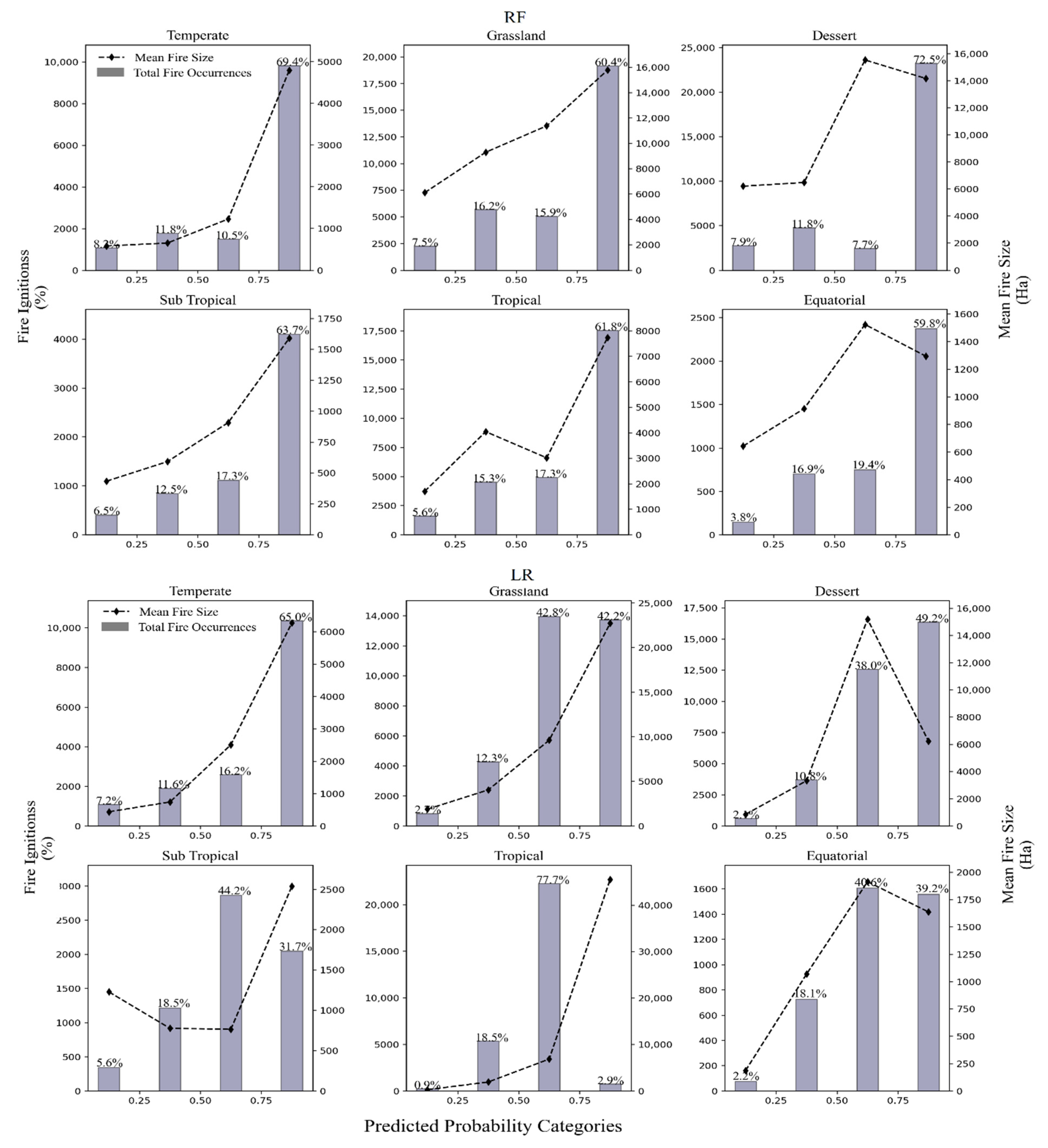
The models predicted probabilities from 0 to 1, with 0 indicating the lowest likelihood of a fire and 1 indicating the highest chance of fire with a large fire size. Thus, we expected lower model probabilities to correspond to either no fire or very few fires with the smallest fire sizes. In contrast, the highest model probabilities would correspond to many fires with the largest fire sizes. To evaluate the efficiency of models, we divided predicted model probabilities into four probability categories, including 0–0.25, 0.26–0.5, 0.51–0.75, and 0.76–1. We calculated and plotted the total percentage of fires and the mean fire size, from the evaluation data, for each predicted probability category. The higher percentages of fires and higher mean fire size in higher probability categories indicated the model’s efficiency in characterizing larger fire sizes towards the higher end of the probability scale [34,68]. Furthermore, we tested the performance of the best model against the fire sizes data from four Black Summer fires (2019–2020) across Australia.
3. Results
3.1. Predictor Importance
Correlation analysis revealed a moderate (0.44) to strong (0.84) correlation between temperature and FFDI, DF and SMD, AWRA-L(s0), and AWRA-L(ss) for all climate zones (Tables S4–S9). The other predictors (relative humidity, rainfall, wind speed, LFMC) displayed a lower correlation with other predictor variables. The predictor importance property of RF did not reveal any specific higher importance for any predictor other than wind speed which showed a slightly better importance score for Temperate and Sub-Tropical climate zones (Figure 4). Furthermore, DF displayed the lowest importance across all climate zones, except for Temperate (Figure 4). We investigated the impact of strongly correlated predictors by leaving out correlated predictors one by one in the model development phase [69]. However, model accuracy did not change. Thus, we retained all the predictors for all climate zones.
3.2. Model Development
Accuracy of Trained Models
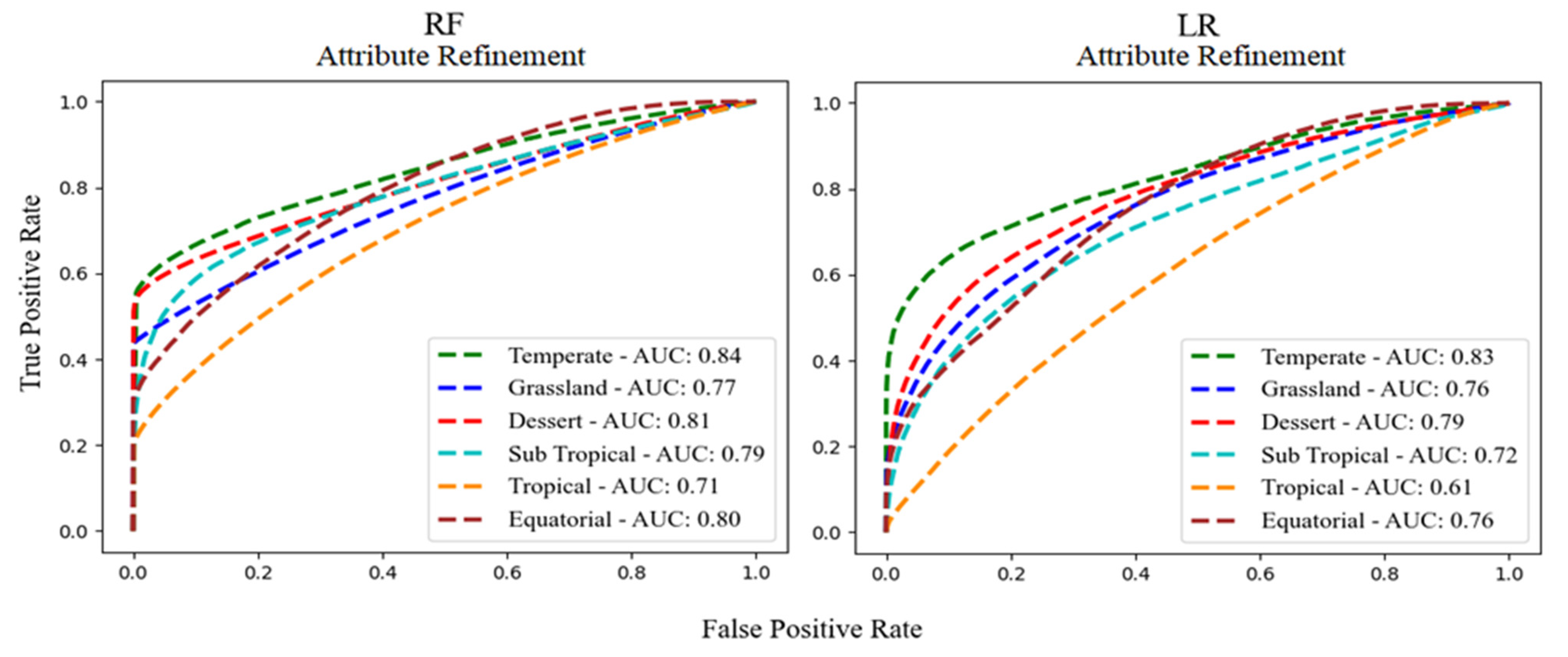
The accuracy of the models trained with all data and class filter methods is explained in the supplementary materials. The models trained with the refined attribute data displayed improved accuracy and higher separability than all data methods but lower than the class filter method. RF models demonstrated high accuracy for the Temperate (0.74) and Dessert (0.76) climate zones, moderate accuracy in the Grasslands (0.69), Sub-Tropical (0.70), and Equatorial (0.71) climate zones, and low accuracy for the Tropical (0.63) climate zone (Table 1). RF displayed a high AUC score for Temperate, Grassland, Dessert, Sub-Tropical, Equatorial, and moderate AUC for Tropical climate zones (Figure 5). The LR models displayed poor accuracy for Tropical (0.58) and low to moderate accuracy for other climate zones (Table 1). In summary, RF showed better results than LR in four climate zones (Dessert, Sub-Tropical, Tropical, and Equatorial).
Overall, the class filter method achieved the best classification accuracy in the development phase (Supplementary materials). Models with refined attribute data (outliers removed) demonstrated reasonable accuracy, and models with all data displayed the lowest classification accuracy. RF demonstrated better classification accuracy than LR in both class filter and attribute refinement methods.
3.3. Evaluation of the Random Forest and Logistic Regression Models (Attribute-Refinement Method)
We expected the models to predict a higher probability as the fire size and number of fires increased. This means as the model probability increases, the chances of starting a fire and that fire growing into a large fire should also increase correspondingly. The three noise-handling methods displayed few dissimilarities in predicting probabilities of fire sizes and fires corresponding to the same probability categories across different climate zones.
RF displayed the best performance with attribute refined data and demonstrated larger mean fire sizes for higher probability categories in three out of six climate zones (Temperate, Grassland, and Sub-Tropical climate zones). However, this trend was not clear for other climate zones, and an approximate pattern of larger mean fire sizes with higher probabilities was observed (Figure 6). Moreover, RF demonstrated excellent characterizing fires, with most fires predicted in the 0.75–1 probability category across all climate zones. LR also demonstrated improved performance with attribute-refined data; however, they showed the majority of fires in the third (0.5–0.75) probability category for most climate zones. Overall, RF displayed better results than LR.
In summary, RF displayed the best results in characterizing most fires and growing these into larger fire sizes with higher probabilities. While the RF method with class filter data performed worst (supplementary materials). The evaluation results revealed that, although the best performing RF (attribute refinement method) models predicted large fire sizes in corresponding high probability categories, the predicted probability categories did not reveal a clear separation between the fire sizes. For example, the highest probability (0.75–1) did not contain only large fire sizes but also a large number of small fire sizes which could be deduced from Figure 6.
4. Discussion
The RF models trained with the fire sizes demonstrated a very good skill in predicting fire size probabilities and the number of fires showing an additional advantage compared to the models trained with fire density or ignitions only in previous studies [23,26,33]. RF models trained with attribute-refined data demonstrated the best skill in predicting fire size probabilities. They predicted larger mean fire sizes with proportionally increasing probability categories in four out of six climate zones (Temperate, Grassland, and Sub-Tropical climate zones). Furthermore, RF characterized the majority of fires in the highest probability category (0.75–1) across all climate zones. The FDI modeling using remote sensing fire sizes and RF presents several advantages over the current fire danger prediction models and recently developed machine learning models. Firstly, using a maximum possible range of fire sizes allowed the models to be trained with the predictor’s data that caused the maximum possible fire sizes in a specific climate zone. This allows the machine learning models to scale and predict probabilities for extreme fire events without extrapolating model results [55]. Although such scaling for machine learning algorithms occurs under the hood, it is still beneficial compared to the deterministic fire danger models such as the McArthur FDIs or the Canadian FWI. Such models rely on extrapolating predictions to predict extreme events because they are calibrated with observations from controlled field experiments [11,71]. Secondly, several recent studies that use machine learning models to build FDIs, have mostly used the fire presence-only [26,33,56], fire density [23], or smaller fire size [27]. These machine learning models gauge the performance of the models by demonstrating that most fires or fire density occurred within the highest predicted probabilities. This study demonstrated that the models trained with a full range of fire sizes provide additional information on the fire size, i.e., fire spread potential, as demonstrated by the increasing mean fire size for high probability categories. Furthermore, since the remote sensing burned area data is continuously being produced, it provides convenient and readily available information that could be used for continuous verification and further improvement of the FDI models such as those developed in this study [7].
The pixelated and modular nature of the fire size probabilities provides the opportunity to be integrated with other probabilistic fire danger aspects. For example, previous studies have shown that fire radiative power (FRP) is linearly related to biomass, surface fuel consumption, and community loss across the southern states of Australia [72,73,74]. Since FRP is continuously available through remote sensing data, it represents another remote sensing variable that could be used to model fuel consumption or fire intensity aspect of fire danger. A probabilistic model could be derived using FRP data from MODIS active fire product (MCD14ML), with similar methods followed in this study with the burned sizes. The probabilistic fire size and FRP can be integrated to create a composite fire risk index, following integration methods from previous studies [75,76,77,78].
Although the machine learning models here predicted fire size probabilities, unlike the deterministic models, the predicted probability categories cannot be directly related to the specific ranges of fire sizes [71]. This lack of relationship could be noted as the RF models predicted a wide range of fire sizes at the higher end of the probability scale. For example, the best RF model’s highest probability category (0.75–1) contained all sizes, from small to the largest possible ones (Figure 6). This demonstrated that the model probabilities could not separate the specific fire size ranges. However, such relationships are essential because, compared to the physical fire characteristic, it is challenging to relate probabilistic outputs to the fire suppression or similar measures required for the operational application of the FDIs. Going forward, the specific range of fire sizes can be related to the predicted probabilistic categories through further research using fine-scale data with various approaches. Such approaches could include: (1) a regression model linking various probability categories to the specific range of fire sizes; (2) an ensemble multiclass supervised machine learning model linking various ranges of fire sizes to classes instead of the probabilities [79]. This latter method is complex and challenging because of the imbalance in classes due to varying fire sizes in the multiple classes [80].
The models trained with all data displayed the lowest performance in the model development and evaluation phases. This is because the lowest accuracy could result when a classifier is trained and evaluated with noisy data, as shown in previous studies [61,81]. The low performance of algorithms was due to both the class and attribute noises in the data, making data overly noisy [62]. Previous studies have highlighted that such noises are challenging to separate due to natural processes [62]. In our case, refining the data noise with both methods demonstrated that informed attribute refinement of the data helped improve the model’s performance much better than the auto removal of misclassified class samples through class filtering [62,82].
The models trained in the class-filter method displayed poor performance in the evaluation phase because they could not predict fire sizes in the intermediate ranges. The models predicted the most fires in the lowest and highest probability categories and placed many fires in the lower probability category. These results do not agree with some previous studies, which demonstrated an increased classification performance with refined data through noise filters [61,81,83,84]. The reason for poor performance is because, along with noisy samples, IPF also removed the correct misclassified data samples carrying important predictors information for fire sizes in the middle ranges, which is one of the drawbacks of filtering class noise [59,81]. Thus, the models trained with class-filter data displayed an inability to predict fires in the intermediate probability categories and placed many fires in the lowest or highest probability categories from the evaluation data.
The models trained with attribute-refined data performed better than other methods. The outliers’ removal helped improve class boundaries, conserved all the fire class (class 1—fire sizes) data, and presented a whole variation of fire sizes to the models contrary to the class-filter method. The naturally occurring outliers in class 0 (no-fire) samples, such as higher temperature and low relative humidity values, typically occur for class 1 (fire sizes) or greater fire danger [14,46]. These outliers complicate the class boundaries and make it difficult for classifiers to distinguish between classes 0 and 1 [63]. Thus, the removal of the outliers from class 0 allowed us to retain all data from class 1 (fire sizes) (Table 1), which helped models perform better by learning from all the variations in the fire sizes, including fires with intermediate fire sizes [85].
The results presented in this study are dependent and representative of the spatial and temporal resolution of the data used to train the models. We used relatively coarse data to train the models; however, the coarse spatial and temporal data averages out the important local variations and their subsequent effects on fire size in some critical factors. For example, the increase in fire size due to blowout potential caused by a sudden change in wind speeds would not be well represented using a coarse spatial and temporal resolution database [46]. The coarse nature of the data also explains why the machine learning algorithms did not give high importance to wind speeds because the wind speed is a highly variant spatial and temporal predictor [30,86]. Fire sizes depend on factors other than those considered in this study, such as fuel connectivity, fuel patchiness, vegetation structure, fuel loads, presence of natural and artificial barriers, variation in wind speeds, and variability in suppression resources employed to control the fires [30,87,88]. However, such datasets are difficult to obtain. LiDAR and line scans may help model and or measure some of these variables at higher spatial and temporal resolutions [89]. The high spatial and temporal resolution could help improve the results by incorporating the refined effects of dynamic variables such as wind speeds and fuel load on fire sizes. Furthermore, the high-resolution data could help establish a relationship between a specific range of fire sizes and the probabilistic model categories discussed above.
5. Conclusions
This study demonstrated that RF models trained with a full range of remote sensing fire sizes could effectively predict fire size probabilities at a regional scale across Australia. The continuous production and convenient availability of remote sensing burned area data provide an easy verification and thus facilitate the continuous improvements of such models. Moreover, the fire size probabilistic predictions could be further integrated with other fire danger aspects such as the FRP probabilities to develop a composite fire danger prediction model. Although the RF models showed great skill in predicting fire size probabilities, these probabilities cannot be directly related to the fire sizes, unlike deterministic fire danger models. However, such a relationship is essential because the probabilities linked to specific fire size ranges could then be related to fire suppression measures and potential damages caused by varying fire sizes, which is necessary for the operational application of such models. The coarse nature of the predictors and response datasets did not help to incorporate the actual effect of some crucial predictors on fire size, such as wind speed. Further research with higher spatial and temporal resolutions would help incorporate the actual effect of the critical predictors into the models. Moreover, a finer resolution of the predictors and response data could help establish a relationship between the predicted probabilities and the specific range of fire sizes.
Supplementary Materials
The Supplementary Materials can be downloaded at https://www.mdpi.com/article/10.3390/fire5050152/s1, Supplementary Methods: S1. Noise handling methods; Supplementary Results: S2. Accuracy of trained models using all data and class filter methods; S3. Evaluation of the random forest and logistic regression models (All data and class-filter methods); Supplementary Tables and Figures: Table S1: Total number of fire size Samples for the three methods used to develop FDIs for respective climate zones; Table S2: Sensitivity (Sens), specificity (Spec) and classification accuracy of RF and LR models with all data method for each climate zones in Australia. Class 0 is no-fire and class 1 is fire class; Table S3: Sensitivity (Sens), specificity (Spec) and classification accuracy of RF and LR models with class filter method (noisy class samples filtered with IPF) across all climate zones in Australia. Class 0 is no-fire and class 1 is fire class; Table S4: Correlation matrix of predictors and response variable for Temperate climate zone; Table S5: Correlation matrix of predictors and response variable for Grassland climate zone; Table S6: Correlation matrix of predictors and response variable for Dessert climate zone; Table S7: Correlation matrix of predictors and response variable for Sub-Tropical climate zone; Table S8: Correlation matrix of predictors and response variable for Tropical climate zone; Table S9: Correlation matrix of predictors and response variable for Equatorial climate zone; Figure S1: Scatter plots of temperature, relative humidity and wind speed against fire sizes for all climate zones; Figure S2: ROC and the respective AUC of class 1 (fire sizes) for RF (top) and LR (bottom) models trained with all data and class filtered data; Figure S3: Evaluation of the RF and LR models developed with all-data. Model predicted probabilities in four categories are shown with the total number of fire ignitions and mean fire sizes; Figure S4: Evaluation of the RF and LR models developed with class filter data (data filtered with IPF). Model predicted probabilities in four categories are shown with the total number of fire ignitions and mean fire sizes. References [59,60,61,62,83,90] is cited in the Supplementary Materials.
Author Contributions
Conceptualization, S.U.S. and M.Y.; methodology, S.U.S.; software, S.U.S.; validation, M.Y., A.I.J.M.V.D. and G.J.C.; formal analysis, S.U.S., M.Y.; investigation, S.U.S. and M.Y.; resources, S.U.S. and M.Y.; data curation, S.U.S.; writing—original draft preparation, S.U.S.; writing—review and editing, S.U.S., M.Y., A.I.J.M.V.D. and G.J.C.; visualization, S.U.S., M.Y., A.I.J.M.V.D. and G.J.C.; supervision, M.Y., A.I.J.M.V.D. and G.J.C.; project administration, S.U.S. and M.Y.; funding acquisition. All authors have read and agreed to the published version of the manuscript.
Funding
This research received no external funding.
Data Availability Statement
Data and the code can be freely provided by the corresponding author on request.
Acknowledgments
The authors thank Gianluca Scortechini, and Peter Hairsine (Fenner School of Environment and Society, Australian National University) who helped compute the daily wind speed data and improve the quality of this manuscript, respectively. We also thank Saeed Anwar, Research Scientist, Imaging and Computer Vision, CSIRO, for his technical advice on using Random Forests, which helped improve the results.
Conflicts of Interest
The authors declare no conflict of interest.
References
- Sharples, J.J.; Cary, G.J.; Fox-Hughes, P.; Mooney, S.; Evans, J.P.; Fletcher, M.-S.; Fromm, M.; Grierson, P.F.; McRae, R.; Baker, P. Natural hazards in Australia: Extreme bushfire. Clim. Chang. 2016, 139, 85–99. [Google Scholar] [CrossRef]
- Ashe, B.; McAneney, K.J.; Pitman, A. Total cost of fire in Australia. J. Risk Res. 2009, 12, 121–136. [Google Scholar] [CrossRef]
- Bowman, D.; Williamson, G.; Yebra, M.; Lizundia-Loiola, J.; Pettinari, M.L.; Shah, S.; Bradstock, R.; Chuvieco, E. Wildfires: Australia Needs National Monitoring Agency; Nature Publishing Group: Berlin/Heidelberg, Germany, 2020. [Google Scholar]
- Filkov, A.I.; Ngo, T.; Matthews, S.; Telfer, S.; Penman, T.D. Impact of Australia’s catastrophic 2019/20 bushfire season on communities and environment. Retrospective analysis and current trends. J. Saf. Sci. Resil. 2020, 1, 44–56. [Google Scholar] [CrossRef]
- Cruz, M.G.; Gould, J. Field-based fire behaviour research: Past and future roles. In Proceedings of the Proceedings of the 18th World IMACS Congress and MODSIM09 International Congress on Modelling and Simulation’, Cairns, Australia, 13–17 July 2009; pp. 247–253. [Google Scholar]
- McRae, R.; Sharples, J. A conceptual framework for assessing the risk posed by extreme bushfires. Aust. J. Emerg. Manag. 2011, 26, 47. [Google Scholar]
- Claire, S.Y.; Jeffrey, D.K.; Robin, H. Fire Danger Indices: Current Limitations and a Pathway to Better Indices; Bushfire and Natural Hazards CRC: Melbourne, Australia, 2014.
- Dutta, R.; Das, A.; Aryal, J. Big data integration shows Australian bush-fire frequency is increasing significantly. R. Soc. Open Sci. 2016, 3, 150241. [Google Scholar] [CrossRef]
- Matthews, S.; Fox-Hughes, P.; Grootemaat, S.; Hollis, J.; Kenny, B.; Sauvage, S. Australian Fire Danger Rating System; Research Prototype; NSW Rural Fire Serrvice: Lindcombe, NSW, Australia, 2019; p. 384.
- Van Dijk, A.I.; Yebra, M.; Cary, G.J.; Shah, S. Towards Comprehensive Characterisation of Flammability and Fire Danger; Bushfire and Natural Hazards CRC AFAC19: Melbourne, VIC, Australia, 2019.
- Sullivan, A.L. Wildland surface fire spread modelling, 1990–2007. 2: Empirical and quasi-empirical models. Int. J. Wildland Fire 2009, 18, 387–403. [Google Scholar] [CrossRef]
- Bradshaw, L.S.; Deeming, J.E.; Burgan, R.E.; Cohen, J.D. The 1978 National Fire-Danger Rating System: Technical Documentation; US Department of Agriculture, Forest Service, Intermountain Forest and Range Experiment Station: Ogeden, UT, USA, 1984.
- Albini, F.A. Estimating Wildfire Behavior and Effects; US Department of Agriculture, Forest Service, Intermountain Forest and Range Experiment Station: Ogeden, UT, USA, 1976.
- Van Wagner, C.E. Structure of the Canadian Forest fire Weather Index; Environment Canada, Forestry Service: Ottawa, ON, USA, 1974; Volume 1333. [Google Scholar]
- McArthur, A.G. Fire Behaviour in Eucalypt Forests; Forestry and Timber Bureau: Yarralumla, Australia, 1967. [Google Scholar]
- Tolhurst, K.; Street, W.; Creswick, V. Report on Fire Danger Ratings and Public Warning; Department of Forest and Ecosystem Science, University of Melbourne: Creswick, Australia, 2010. [Google Scholar]
- Storey, M.A.; Price, O.F.; Sharples, J.J.; Bradstock, R.A. Drivers of long-distance spotting during wildfires in south-eastern Australia. Int. J. Wildland Fire 2020, 29, 459–472. [Google Scholar] [CrossRef]
- Levin, N.; Yebra, M.; Phinn, S. Unveiling the Factors Responsible for Australia’s Black Summer Fires of 2019/2020. Fire 2021, 4, 58. [Google Scholar] [CrossRef]
- Giglio, L.; Boschetti, L.; Roy, D.P.; Humber, M.L.; Justice, C.O. The Collection 6 MODIS burned area mapping algorithm and product. Remote Sens. Environ. 2018, 217, 72–85. [Google Scholar] [CrossRef]
- Giglio, L.; Schroeder, W.; Hall, J.V.; Justice, C.O. Modis collection 6 active fire product user’s guide revision A. In Department of Geographical Sciences; University of Maryland: College Park, MD, USA, 2015. [Google Scholar]
- Massada, A.B.; Syphard, A.D.; Stewart, S.I.; Radeloff, V.C. Wildfire ignition-distribution modelling: A comparative study in the Huron–Manistee National Forest, Michigan, USA. Int. J. Wildland Fire 2013, 22, 174–183. [Google Scholar] [CrossRef]
- Ngoc Thach, N.; Bao-Toan Ngo, D.; Xuan-Canh, P.; Hong-Thi, N.; Hang Thi, B.; Nhat-Duc, H.; Dieu, T.B. Spatial pattern assessment of tropical forest fire danger at Thuan Chau area (Vietnam) using GIS-based advanced machine learning algorithms: A comparative study. Ecol. Inform. 2018, 46, 74–85. [Google Scholar] [CrossRef]
- Oliveira, S.; Oehler, F.; San-Miguel-Ayanz, J.; Camia, A.; Pereira, J.M.C. Modeling spatial patterns of fire occurrence in Mediterranean Europe using Multiple Regression and Random Forest. For. Ecol. Manag. 2012, 275, 117–129. [Google Scholar] [CrossRef]
- Preisler, H.K.; Burgan, R.E.; Eidenshink, J.C.; Klaver, J.M.; Klaver, R.W. Simulation models mainly use two types of propagation algorithms based on the type of GIS data, i.e., vector and rasters, to implement the simulation models. Int. J. Wildland Fire 2009, 18, 508–516. [Google Scholar] [CrossRef]
- Sakr, G.E.; Elhajj, I.H.; Mitri, G. Efficient forest fire occurrence prediction for developing countries using two weather parameters. Eng. Appl. Artif. Intell. 2011, 24, 888–894. [Google Scholar] [CrossRef]
- Tien Bui, D.; Le, H.V.; Hoang, N.-D. GIS-based spatial prediction of tropical forest fire danger using a new hybrid machine learning method. Ecol. Inform. 2018, 48, 104–116. [Google Scholar] [CrossRef]
- Cortez, P.; Morais, A.d.J.R. A Data Mining Approach to Predict Forest Fires Using Meteorological Data; Associação Portuguesa para a Inteligência Artificial (APPIA): Guimarães, Portugal, 2007. [Google Scholar]
- Bradstock, R.A.; Cohn, J.; Gill, A.M.; Bedward, M.; Lucas, C. Prediction of the probability of large fires in the Sydney region of south-eastern Australia using fire weather. Int. J. Wildland Fire 2010, 18, 932–943. [Google Scholar] [CrossRef]
- Laurent, P.; Mouillot, F.; Moreno, M.V.; Yue, C.; Ciais, P. Varying relationships between fire radiative power and fire size at a global scale. Biogeosciences 2019, 16, 275–288. [Google Scholar] [CrossRef]
- Fang, L.; Yang, J.; Zu, J.; Li, G.; Zhang, J. Quantifying influences and relative importance of fire weather, topography, and vegetation on fire size and fire severity in a Chinese boreal forest landscape. For. Ecol. Manag. 2015, 356, 2–12. [Google Scholar] [CrossRef]
- Podur, J.J.; Martell, D.L. The influence of weather and fuel type on the fuel composition of the area burned by forest fires in Ontario, 1996–2006. Ecol. Appl. 2009, 19, 1246–1252. [Google Scholar] [CrossRef]
- Cary, G.J.; Keane, R.E.; Gardner, R.H.; Lavorel, S.; Flannigan, M.D.; Davies, I.D.; Li, C.; Lenihan, J.M.; Rupp, T.S.; Mouillot, F. Comparison of the sensitivity of landscape-fire-succession models to variation in terrain, fuel pattern, climate and weather. Landsc. Ecol. 2006, 21, 121–137. [Google Scholar] [CrossRef]
- Pourghasemi, H.R. GIS-based forest fire susceptibility mapping in Iran: A comparison between evidential belief function and binary logistic regression models. Scand. J. For. Res. 2016, 31, 80–98. [Google Scholar] [CrossRef]
- Nami, M.H.; Jaafari, A.; Fallah, M.; Nabiuni, S. Spatial prediction of wildfire probability in the Hyrcanian ecoregion using evidential belief function model and GIS. Int. J. Environ. Sci. Technol. 2017, 15, 373–384. [Google Scholar] [CrossRef]
- Vermote, E.F.; El Saleous, N.Z.; Justice, C.O. Atmospheric correction of MODIS data in the visible to middle infrared: First results. Remote Sens. Environ. 2002, 83, 97–111. [Google Scholar] [CrossRef]
- Giglio, L.; Boschetti, L.; Roy, D.; Hoffmann, A.A.; Humber, M.; Hall, J.V. Collection 6 MODIS Burned Area Product User’s Guide Version 1.0; NASA EOSDIS Land Processes DAAC: Sioux Falls, SD, USA, 2016.
- Jones, D.A.; Wang, W.; Fawcett, R. High-quality spatial climate data-sets for Australia. Aust. Meteorol. Oceanogr. J. 2009, 58, 233. [Google Scholar] [CrossRef]
- Raupach, M.; Briggs, P.; Haverd, V.; King, E.; Paget, M.; Trudinger, C. Australian Water Availability Project; CSIRO Marine and Atmospheric Research: Canberra, Australia, 2012. [Google Scholar]
- Muñoz Sabater, J. ERA5-Land Hourly Data from 1981 to Present. Available online: https://cds.climate.copernicus.eu/cdsapp#!/dataset/10.24381/cds.e2161bac?tab=overview (accessed on 3 July 2022).
- Nolan, R.H.; Resco de Dios, V.; Boer, M.M.; Caccamo, G.; Goulden, M.L.; Bradstock, R.A. Predicting dead fine fuel moisture at regional scales using vapour pressure deficit from MODIS and gridded weather data. Remote Sens. Environ. 2016, 174, 100–108. [Google Scholar] [CrossRef]
- Mount, A. The Derivation and Testing of a Soil Dryness Index Using Run-Off Data; Tasmania Forestry Commission: Hobart, Australia, 1972. [Google Scholar]
- Finkele, K.; Graham, A.M.l.; Grant, B.; David, A.J. National Daily Gridded Soil Moisture Deficit and Drought Factors for Use in Prediction of Forest Fire Danger Index in Australia; Bureau of Meteorology Research Centre: Melbourne, Australia, 2006.
- Keetch, J.J.; Byram, G.M. A Drought Index for Forest Fire Control; Research Paper SE-38; US Department of Agriculture, Forest Service, Southeastern Forest Experiment Station: Asheville NC, USA, 1968; Volume 38, 35p. [Google Scholar]
- Noble, I.; Gill, A.; Bary, G. McArthur’s fire-danger meters expressed as equations. Aust. J. Ecol. 1980, 5, 201–203. [Google Scholar] [CrossRef]
- Dowdy, A.J. Climatological Variability of Fire Weather in Australia. J. Appl. Meteorol. Climatol. 2018, 57, 221–234. [Google Scholar] [CrossRef]
- Cruz, M.G.; Gould, J.S.; Alexander, M.E.; Sullivan, A.L.; McCaw, W.L.; Matthews, S. A Guide to Rate of Fire Spread Models for Australian Vegetation, Revised ed.; CSIRO, Land and Water, AFAC: Clayton, Australia, 2015. [Google Scholar]
- Kumar, V.; Dharssi, I. Evaluation and calibration of a high-resolution soil moisture product for wildfire prediction and management. Agric. For. Meteorol. 2019, 264, 27–39. [Google Scholar]
- Frost, A.; Ramchurn, A.; Smith, A. The Australian Landscape Water Balance model (AWRA-L v6). Technical Description of the Australian Water Resources Assessment Landscape Model; Bureau of Meteorology: Melbourne, Australia, 2018; 6.
- Vaze, J.; Viney, N.; Stenson, M.; Renzullo, L.; Van Dijk, A.; Dutta, D.; Crosbie, R.; Lerat, J.; Penton, D.; Vleeshouwer, J. The australian water resource assessment modelling system (awra). In Proceedings of the 20th International Congress on Modelling and Simulation, Adelaide, Australia, 1–6 December 2013; pp. 1–6. [Google Scholar]
- Yebra, M.; Quan, X.; Riaño, D.; Rozas Larraondo, P.; van Dijk, A.I.J.M.; Cary, G.J. A fuel moisture content and flammability monitoring methodology for continental Australia based on optical remote sensing. Remote Sens. Environ. 2018, 212, 260–272. [Google Scholar] [CrossRef]
- Beck, H.E.; Zimmermann, N.E.; McVicar, T.R.; Vergopolan, N.; Berg, A.; Wood, E.F. Present and future Köppen-Geiger climate classification maps at 1-km resolution. Sci. Data 2018, 5, 180214. [Google Scholar] [CrossRef]
- Sullivan, A.L.; McCaw, W.L.; Cruz, M.G.; Matthews, S.; Ellis, P.F. Fuel, fire weather and fire behaviour in Australian ecosystems. In Flammable Australia: Fire regimes, Biodiversity and Ecosystems in a Changing World; CSIRO Publishing: Collingwood, VIC, Australia, 2012; pp. 51–77. [Google Scholar]
- Luke, R.H.; McArthur, A.G. Bushfires in Australia; Australian Government Publishing Service for CSIRO: Clayton, Australia, 1978. [Google Scholar]
- Pourtaghi, Z.S.; Pourghasemi, H.R.; Aretano, R.; Semeraro, T. Investigation of general indicators influencing on forest fire and its susceptibility modeling using different data mining techniques. Ecol. Indic. 2016, 64, 72–84. [Google Scholar] [CrossRef]
- Breiman, L. Random forests. Mach. Learn. 2001, 45, 5–32. [Google Scholar] [CrossRef] [Green Version]
- Arpaci, A.; Malowerschnig, B.; Sass, O.; Vacik, H. Using multi variate data mining techniques for estimating fire susceptibility of Tyrolean forests. Appl. Geogr. 2014, 53, 258–270. [Google Scholar] [CrossRef]
- Catry, F.X.; Rego, F.C.; Bação, F.L.; Moreira, F. Modeling and mapping wildfire ignition risk in Portugal. Int. J. Wildland Fire 2009, 18, 921–931. [Google Scholar] [CrossRef]
- Martínez, J.; Vega-Garcia, C.; Chuvieco, E. Human-caused wildfire risk rating for prevention planning in Spain. J. Environ. Manag. 2009, 90, 1241–1252. [Google Scholar] [CrossRef]
- Gupta, S.; Gupta, A. Dealing with noise problem in machine learning data-sets: A systematic review. Procedia Comput. Sci. 2019, 161, 466–474. [Google Scholar] [CrossRef]
- Verbaeten, S.; Van Assche, A. Ensemble methods for noise elimination in classification problems. In Proceedings of the International Workshop on Multiple Classifier Systems, Nanjing, China, 15–17 May 2003; pp. 317–325. [Google Scholar]
- Sáez, J.A.; Galar, M.; Luengo, J.; Herrera, F. INFFC: An iterative class noise filter based on the fusion of classifiers with noise sensitivity control. Inf. Fusion 2016, 27, 19–32. [Google Scholar] [CrossRef]
- Zhu, X.; Wu, X. Class noise vs. attribute noise: A quantitative study. Artif. Intell. Rev. 2004, 22, 177–210. [Google Scholar] [CrossRef]
- Li, W.; Mo, W.; Zhang, X.; Squiers, J.J.; Lu, Y.; Sellke, E.W.; Fan, W.; DiMaio, J.M.; Thatcher, J.E. Outlier detection and removal improves accuracy of machine learning approach to multispectral burn diagnostic imaging. J. Biomed. Opt. 2015, 20, 121305. [Google Scholar] [CrossRef]
- Tolhurst, K.; Shields, B.; Chong, D. Phoenix: Development and application of a bushfire risk management tool. Aust. J. Emerg. Manag. 2008, 23, 47. [Google Scholar]
- Pedregosa, F.; Varoquaux, G.; Gramfort, A.; Michel, V.; Thirion, B.; Grisel, O.; Blondel, M.; Prettenhofer, P.; Weiss, R.; Dubourg, V. Scikit-learn: Machine learning in Python. J. Mach. Learn. Res. 2011, 12, 2825–2830. [Google Scholar]
- Witten, I.H.; Frank, E.; Mark, A.H. Data Mining: Practical Machine Learning Tools and Techniques, 3rd ed.; Morgan, Kaufmann: Burlington, MA, USA, 2011; Volume 31, pp. 76–77. [Google Scholar]
- Fernandes, A.M.; Utkin, A.B.; Lavrov, A.V.; Vilar, R.M. Development of neural network committee machines for automatic forest fire detection using lidar. Pattern Recognit. 2004, 37, 2039–2047. [Google Scholar] [CrossRef]
- Jaafari, A.; Zenner, E.K.; Panahi, M.; Shahabi, H. Hybrid artificial intelligence models based on a neuro-fuzzy system and metaheuristic optimization algorithms for spatial prediction of wildfire probability. Agric. For. Meteorol. 2019, 266–267, 198–207. [Google Scholar] [CrossRef]
- Lei, J.; G’Sell, M.; Rinaldo, A.; Tibshirani, R.J.; Wasserman, L. Distribution-free predictive inference for regression. J. Am. Stat. Assoc. 2018, 113, 1094–1111. [Google Scholar] [CrossRef] [Green Version]
- Fox, P.H.; Yebra, M.; Shokirov, S.; Kumar, V.; Dowdy, A.; Hope, P.; Peace, M.; Narsey, S.; Delage, F.; Zhang, H. Soil and fuel moisture precursors of fire activity during the 2019–20 fire season, in comparison to previous seasons; Bushfire and Natural Hazards CRC: Melbourne, Australia, 2021.
- Storey, M.A.; Bedward, M.; Price, O.F.; Bradstock, R.A.; Sharples, J.J. Derivation of a Bayesian fire spread model using large-scale wildfire observations. Environ. Model. Softw. 2021, 144, 105127. [Google Scholar] [CrossRef]
- Harris, S.; Anderson, W.; Kilinc, M.; Fogarty, L. The relationship between fire behaviour measures and community loss: An exploratory analysis for developing a bushfire severity scale. Nat. Hazards 2012, 63, 391–415. [Google Scholar] [CrossRef]
- Wooster, M.J.; Roberts, G.; Perry, G.; Kaufman, Y. Retrieval of biomass combustion rates and totals from fire radiative power observations: FRP derivation and calibration relationships between biomass consumption and fire radiative energy release. J. Geophys. Res. Atmos. 2005, 110, 1–24. [Google Scholar] [CrossRef]
- Hudak, A.T.; Dickinson, M.B.; Bright, B.C.; Kremens, R.L.; Loudermilk, E.L.; O’Brien, J.J.; Hornsby, B.S.; Ottmar, R.D. Measurements relating fire radiative energy density and surface fuel consumption–RxCADRE 2011 and 2012. Int. J. Wildland Fire 2016, 25, 25–37. [Google Scholar] [CrossRef]
- Gai, C.; Weng, W.; Yuan, H. GIS-based forest fire risk assessment and mapping. In Proceedings of the 2011 Fourth International Joint Conference on Computational Sciences and Optimization (CSO), Kunming, China, 15–19 April 2011; pp. 1240–1244. [Google Scholar]
- Setiawan, I.; Mahmud, A.R.; Mansor, S.; Mohamed Shariff, A.R.; Nuruddin, A.A. GIS-grid-based and multi-criteria analysis for identifying and mapping peat swamp forest fire hazard in Pahang, Malaysia. Disaster Prev. Manag. Int. J. 2004, 13, 379–386. [Google Scholar] [CrossRef]
- Chuvieco, E.; Allgöwer, B.; Salas, J. Integration of physical and human factors in fire danger assessment. In Wildland Fire Danger Estimation and Mapping: The Role of Remote Sensing Data; World Scientific Publishing Co. Pte. Ltd.: Singapore, 2003; pp. 197–218. [Google Scholar]
- Chuvieco, E.; Aguado, I.; Yebra, M.; Nieto, H.; Salas, J.; Martín, M.P.; Vilar, L.; Martínez, J.; Martín, S.; Ibarra, P.; et al. Development of a framework for fire risk assessment using remote sensing and geographic information system technologies. Ecol. Model. 2010, 221, 46–58. [Google Scholar] [CrossRef]
- O’Brien, R.; Ishwaran, H. A random forests quantile classifier for class imbalanced data. Pattern Recognit. 2019, 90, 232–249. [Google Scholar] [CrossRef] [PubMed]
- Zhang, Z.; Krawczyk, B.; Garcia, S.; Rosales-Perez, A.; Herrera, F. Empowering one-vs-one decomposition with ensemble learning for multi-class imbalanced data. Knowl.-Based Syst. 2016, 106, 251–263. [Google Scholar] [CrossRef]
- Brodley, C.E.; Friedl, M.A. Identifying mislabeled training data. J. Artif. Intell. Res. 1999, 11, 131–167. [Google Scholar] [CrossRef]
- Zhao, Q.; Nishida, T. Using qualitative hypotheses to identify inaccurate data. J. Artif. Intell. Res. 1995, 3, 119–145. [Google Scholar] [CrossRef] [Green Version]
- Khoshgoftaar, T.M.; Rebours, P. Improving software quality prediction by noise filtering techniques. J. Comput. Sci. Technol. 2007, 22, 387–396. [Google Scholar] [CrossRef]
- Khoshgoftaar, T.M.; Zhong, S.; Joshi, V. Enhancing software quality estimation using ensemble-classifier based noise filtering. Intell. Data Anal. 2005, 9, 3–27. [Google Scholar] [CrossRef]
- Li, P.; Rao, X.; Blase, J.; Zhang, Y.; Chu, X.; Zhang, C. Cleanml: A benchmark for joint data cleaning and machine learning [experiments and analysis]. arXiv 2019, arXiv:1904.09483. [Google Scholar]
- Ruffault, J.; Moron, V.; Trigo, R.M.; Curt, T. Daily synoptic conditions associated with large fire occurrence in Mediterranean France: Evidence for a wind-driven fire regime. Int. J. Climatol. 2017, 37, 524–533. [Google Scholar] [CrossRef]
- Meyn, A.; White, P.S.; Buhk, C.; Jentsch, A. Environmental drivers of large, infrequent wildfires: The emerging conceptual model. Prog. Phys. Geogr. 2007, 31, 287–312. [Google Scholar] [CrossRef]
- Parisien, M.-A.; Parks, S.A.; Krawchuk, M.A.; Flannigan, M.D.; Bowman, L.M.; Moritz, M.A. Scale-dependent controls on the area burned in the boreal forest of Canada, 1980–2005. Ecol. Appl. 2011, 21, 789–805. [Google Scholar] [CrossRef]
- Liao, Z.; Van Dijk, A.I.; He, B.; Larraondo, P.R.; Scarth, P.F. Woody vegetation cover, height and biomass at 25-m resolution across Australia derived from multiple site, airborne and satellite observations. Int. J. Appl. Earth Obs. Geoinf. 2020, 93, 102209. [Google Scholar] [CrossRef]
- Rodriguez, J.D.; Perez, A.; Lozano, J.A. Sensitivity analysis of k-fold cross validation in prediction error estimation. IEEE Trans. Pattern Anal. Mach. Intell. 2009, 32, 569–575. [Google Scholar] [CrossRef] [PubMed]
Figure 1.
Stratification of Australia into (a) vegetation types based on temperature and rainfall using the Koppen-Geiger regional classification (b) fire seasons.
Figure 1.
Stratification of Australia into (a) vegetation types based on temperature and rainfall using the Koppen-Geiger regional classification (b) fire seasons.

Figure 2.
Methodology flowchart. RF: Random Forest, LR: Logistic Regresion, CV: Cross Validation.

Figure 3.
Fire size samples shown on log10 scale for six climate zones across Australia, extracted from fire seasons: (a) 2000–2016 (model development); (b) 2017–2020 (model evaluation). The lower and upper boundary of boxes represent 25th and 75th percentiles, respectively. Whiskers extended to 1.5 times interquartile ranges. The blue line in boxes represent median, red diamonds represent mean fire size and black circular dots represent outliers.

Figure 4.
Predictor importance for predicting fire sizes, computed with feature (predictor) importance property of RF for all climate zones. T: Temperature, RH: Relative humidity, WS: Wind speed, DF: Drought factor, SMD: Soil moisture deficit, FFDI: Forest fire danger index, LFMC: Live fuel moisture content.

Figure 5.
ROC and the respective AUC of class 1 (fire sizes) for RF and LR models trained with attribute refined data.
Figure 5.
ROC and the respective AUC of class 1 (fire sizes) for RF and LR models trained with attribute refined data.

Figure 6.
Evaluation of the RF and LR models developed with attribute-refined data (Outlier removed from Temperature and relative humidity predictors in class 0 (no-fire class)). The model predicted probabilities in four categories are shown with the total number of fire ignitions and mean fire sizes. The figures on top of each bar denotes the percentage of a number of fires in each probability category out of the overall total number of fires.

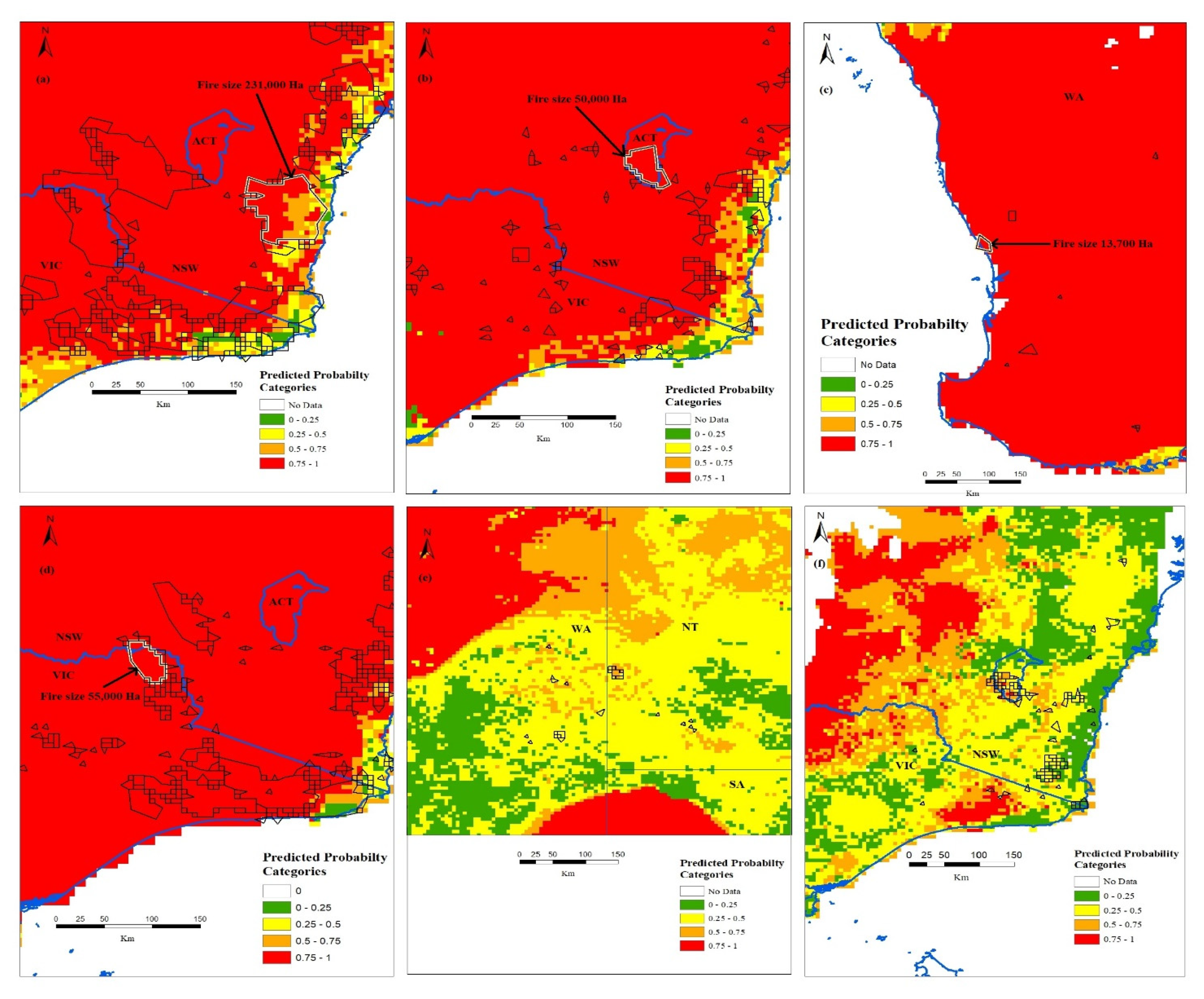
Figure 7.
Predicted fire size probability categories vs. the fire sizes (shown in black outline polygons) for the Black Summer fires (2019–2020, Australia). The first four images also include fire sizes reported by Fox, et al. [70] (shown in white outline and indicated by the arrow): (a) Badja Forest Road, (NSW) fire burnt an area of approximately 231,000 Ha in the first week of January (1–8) 2019; (b) Orroral Valley fire, (ACT) burnt an area of around 50,000 Ha from 25 January–01 February 2020; (c) Yancep fire (WA) burnt an area of approximately 13,700 Ha from 11–18 December 2019; (d) Corryong fire (VIC) burnt an area of around 55,000 (Ha) in the last week of December (27–31) 2019. The predicted probability categories vs. the fire sizes shown here are on weekly scale. Thus the total fire area in these fire events may vary in total quantity and duration as compared to those mentioned in [70], because of the difference in duration of the time the fires kept burning. Note that the majority of the model predictions in the first four images fall in the highest probability category (0.75–1) because of the extreme fire danger conditions in the 2019–2020 fire season. The last two images show randomly selected images with lower predicted fire size probabilities and corresponding fire sizes: (e) 1–8 January 2020; (f) 10–17 February 2020.


Table 1.
Sensitivity (Sens), specificity (Spec) and classification accuracy of RF and LR models with attribute refinement method (outliers removed from temperature and relative humidity predictors in class 0 (no-fire class)) across all climate zones in Australia. Class 0 is no-fire and class 1 is fire size class.
| Climate Zone | RF | LR | ||||||||
|---|---|---|---|---|---|---|---|---|---|---|
| Class 0 | Class 1 | Accuracy | Class 0 | Class 1 | Accuracy | |||||
| Sens | Spec | Sens | Spec | Sens | Spec | Sens | Spec | |||
| Temperate | 0.71 | 0.76 | 0.77 | 0.72 | 0.74 | 0.73 | 0.75 | 0.75 | 0.73 | 0.74 |
| Grasslands | 0.72 | 0.67 | 0.66 | 0.72 | 0.69 | 0.67 | 0.68 | 0.71 | 0.70 | 0.69 |
| Dessert | 0.85 | 0.71 | 0.66 | 0.82 | 0.76 | 0.70 | 0.71 | 0.72 | 0.71 | 0.71 |
| Sub-Tropical | 0.64 | 0.72 | 0.76 | 0.68 | 0.70 | 0.62 | 0.66 | 0.69 | 0.65 | 0.66 |
| Tropical | 0.56 | 0.66 | 0.71 | 0.62 | 0.63 | 0.59 | 0.49 | 0.67 | 0.57 | 0.58 |
| Equatorial | 0.70 | 0.71 | 0.71 | 0.70 | 0.71 | 0.62 | 0.71 | 0.74 | 0.66 | 0.68 |
Publisher’s Note: MDPI stays neutral with regard to jurisdictional claims in published maps and institutional affiliations. |
© 2022 by the authors. Licensee MDPI, Basel, Switzerland. This article is an open access article distributed under the terms and conditions of the Creative Commons Attribution (CC BY) license (https://creativecommons.org/licenses/by/4.0/).
Share and Cite
MDPI and ACS Style
Shah, S.U.; Yebra, M.; Van Dijk, A.I.J.M.; Cary, G.J. A New Fire Danger Index Developed by Random Forest Analysis of Remote Sensing Derived Fire Sizes. Fire 2022, 5, 152. https://doi.org/10.3390/fire5050152
AMA Style
Shah SU, Yebra M, Van Dijk AIJM, Cary GJ. A New Fire Danger Index Developed by Random Forest Analysis of Remote Sensing Derived Fire Sizes. Fire. 2022; 5(5):152. https://doi.org/10.3390/fire5050152
Chicago/Turabian StyleShah, Sami Ullah, Marta Yebra, Albert I. J. M. Van Dijk, and Geoffrey J. Cary. 2022. "A New Fire Danger Index Developed by Random Forest Analysis of Remote Sensing Derived Fire Sizes" Fire 5, no. 5: 152. https://doi.org/10.3390/fire5050152