
Practical Application of Deep Reinforcement Learning to Optimal Trade Execution

Qraft Technologies, Inc., 3040 Three IFC, 10 Gukjegeumyung-ro, Yeongdeungpo-gu, Seoul 07326, Republic of Korea
*
Authors to whom correspondence should be addressed.
†
These authors contributed equally to this work. Author ordering is randomly determined.
FinTech 2023, 2(3), 414-429; https://doi.org/10.3390/fintech2030023
Submission received: 9 May 2023
/
Revised: 16 June 2023
/
Accepted: 21 June 2023
/
Published: 29 June 2023
(This article belongs to the Special Issue Advances in Analytics and Intelligent System)
Abstract
:Although deep reinforcement learning (DRL) has recently emerged as a promising technique for optimal trade execution, two problems still remain unsolved: (1) the lack of a generalized model for a large collection of stocks and execution time horizons; and (2) the inability to accurately train algorithms due to the discrepancy between the simulation environment and real market. In this article, we address the two issues by utilizing a widely used reinforcement learning (RL) algorithm called proximal policy optimization (PPO) with a long short-term memory (LSTM) network and by building our proprietary order execution simulation environment based on historical level 3 market data of the Korea Stock Exchange (KRX). This paper, to the best of our knowledge, is the first to achieve generalization across 50 stocks and across an execution time horizon ranging from 165 to 380 min along with dynamic target volume. The experimental results demonstrate that the proposed algorithm outperforms the popular benchmark, the volume-weighted average price (VWAP), highlighting the potential use of DRL for optimal trade execution in real-world financial markets. Furthermore, our algorithm is the first commercialized DRL-based optimal trade execution algorithm in the South Korea stock market.
1. Introduction
Electronic trading has gradually become the dominant form of trading in the modern financial market, comprising the majority of the total trading volumes. As a subfield of electronic trading, optimal trade execution has also become a crucial concept in financial markets. In the problem of optimal trade execution, the goal is to buy (or sell) V shares of a particular stock within a defined time period while minimizing the costs that are associated with trading. When executing a large order, however, submitting one large order would incur slippage because of its market impacts, which forces the large order to be split up into several smaller orders. The smaller orders would then be submitted in the hopes of being sequentially executed over time. Sequential decision making is a natural fit for reinforcement learning (RL) as it is mainly modeled as a Markov decision process (MDP) where the next state only depends on the current state and action taken. For this reason, there have been several studies that apply RL in optimal trade execution problems. Nevmyvaka et al. (2006) [1] took advantage of RL to decide the optimal price level to reposition the remaining inventory based on real-time market conditions. Hendricks and Wilcox (2014) [2] extended the standard model of Almgren and Chriss (2001) [3] by incorporating market microstructure elements, demonstrating another way to leverage RL in addressing the problem of optimal trade execution.
However, with the recent advances in neural networks and their ability to learn from data, researchers have turned to more advanced approaches that use deep reinforcement learning (DRL) (Mnih et al. (2013) [4]) for problems that have a wide range of data inputs and market signals.
Dabérius et al. (2019) [5] and Ye et al. (2020) [6]’s studies have led to the successful integration of DRL for optimal trade execution, showing new potential routes for future work. The effectiveness of both value-based and policy gradient DRL algorithms has been demonstrated through the experiments conducted by Ning et al. (2021) [7] and Lin and Beling (2020) [8].
Nevertheless, previous studies that have applied DRL to optimal trade execution have not been successful in bridging the gap between their experimental results and practical utility, making their findings less relevant to real market scenarios.
In order to be applied in the real market, it is imperative for the model to perform well in diverse settings. These could include a wide coverage of different stocks, flexible execution time horizon, and dynamic target volume. Through the use of a detailed setup that integrates DRL algorithms and a vast amount of granular market data, we have achieved effective advancements towards the practical usage of DRL-based optimal trade execution algorithms in the real market.
Table 1 demonstrates how our study developed a generalized DRL model for optimal trade execution that can be utilized in diverse settings by comparing the model with the existing studies in the literature. We focused on the three features of stock group size, execution time horizon, and dynamic target volume, and the specifications in Table 1 denote the coverage of a single trained model. It should be noted that the dynamic target volume implies that there are no preset values for each scenario.
As shown in Table 1, all of the previous studies had either a fixed or short range in the execution time horizon. Moreover, none of the previous studies employed the dynamic target volume. However, fixed or short execution time horizons and preset target volumes are impractical compared with actual execution specifications. This is because the execution time horizon and target volume considerably vary depending on the client or asset manager. Although Hendricks and Wilcox (2014) [2] had a stock group size of 166, their model only works for execution time horizons between 20 and 60 min with two fixed target volumes of 10,000 and 1,000,000 shares. Moreover, our study’s execution time horizon of 165–380 min is the longest in the literature, and our study is the first to employ the dynamic target volume, which signifies the practicality of our model and its ability to be the first to achieve generalization across all three of the features mentioned above.
Additionally, simulating real markets within minimal discrepancy poses a significant challenge, as accurately capturing the market impact and incorporating feedback from all other market participants are nearly impossible (Kyle and Obizhaeva (2018) [11]). Although reasonable assumptions can be incorporated into the simulation logic as in Lin and Beling (2020) [8], such assumptions are more likely to lead to a discrepancy between the simulation environment and the real market. In this regard, we attempted to minimize such assumptions by utilizing level 3 data, which is one of the most granular form of market data, and developed a simulation environment that is highly representative of the real market, as shown in Section 3.2 and Section 3.3. Moreover, the availability of such data allows for the development of a sophisticated Markov decision process (MDP) state and reward designs that lead to the enhanced training of the DRL agent. The details of the state and reward designs can be found in Section 2.3.
Our main contributions in using DRL for optimal trade execution are as follows:
- We set up an order execution simulation environment using level 3 market data to minimize the discrepancy between the environment and the real market during training, which cannot be achieved when using less granular market data.
- We successfully trained a generalized DRL agent that can, on average, outperform the volume-weighted average price (VWAP) of the market for a stock group comprising 50 stocks over an execution time horizon ranging from 165 min to 380 min, which is the longest in the literature; this is accomplished by using the dynamic target volume.
- We formulated a problem setting within the DRL framework in which the agent can choose to pass, submit a market/limit order, modify an outstanding limit order, and choose the volume of the order if the chosen action type is an order.
- We successfully commercialized our algorithm in the South Korea stock market.
Related Work
Researchers from financial domains have shown great interest in the optimal trade execution problem, making it a prominent research topic in the field of algorithmic trading. Bertsimas and Lo (1998) [12] are the pioneers of the problem, and their use of dynamic programming to find an explicit closed-form solution for minimizing trade execution costs was a remarkable achievement. Building onto the research, Almgren and Chriss (2001) [3] introduced the influential Almgren–Chriss model, which concurrently took transaction costs, complex price impact functions, and risk aversion parameters into account. While closed-form solutions can be utilized for trading, they require strong assumptions to be made about the price movements. Consequently, more straightforward strategies such as the time-weighted average price (TWAP) and volume-weighted average price (VWAP) strategies still remain as the default options. Nevertheless, due to their simplicity and inability to adapt, those strategies also struggle to outperform their respective benchmarks when applied in the real market. For this reason, given that reinforcement learning (RL) algorithms can dynamically adapt to the observed market conditions while minimizing transaction costs, RL poses itself as an effective approach for tackling the optimal trade execution problem.
Nevmyvaka et al. (2006) [1] were the first to present the extensive empirical application of RL in the optimal trade execution problem using large-scale data. The authors proposed a model that outputs the relative price at which to reposition all of the remaining inventory. It can be thought of as consecutively modifying any outstanding limit orders with the goal of minimizing implementation shortfall (IS) within a short execution time frame. The authors used historical data from the electronic communication network INET for three stocks, which they split into training and test sets for the time ranges of 12 months and 6 months, respectively. Their execution time horizon ranged from 2 min to 8 min with 5000 fixed shares to execute.
Then, Hendricks and Wilcox (2014) [2] extended the standard model of Almgren and Chriss (2001) [3] by utilizing elements from the market microstructure. Because the Almgren–Chriss framework mainly focuses on the arrival price benchmark, they optimized the number of market orders to submit to be based on the prevailing market conditions. The authors used 12 months of data from the Thomson Reuters Tick History (TRTH) database, which comprises 166 stocks that make up the South African local benchmark index (ALSI). Their execution time horizon ranged from 20 min to 60 min with the target volume ranging from 100,000 to 1,000,000 shares.
While the two previous studies successfully employed Q-learning (Watkins and Dayan (1992) [13]), an RL algorithm, for the purposes of optimal trade execution, the complex dynamics of the financial market and high dimensionality still remain as challenges. With the recent advancements in the field of RL, deep reinforcement learning (DRL) in particular has also gained a lot of popularity in the field of optimal trade execution, wherein the efficacy of neural networks is leveraged as function approximators. Both value-based and policy gradient methods, which are standard approaches in RL, are utilized.
Ning et al. (2021) [7] and Li et al. (2022) [10] employed the extended version of the deep Q-Network (DQN) (Mnih et al. (2015) [14]; in the work of Van Hasselt et al. (2016) [15])that focused on optimal trade execution, by taking advantage of the ability of deep neural networks to learn from a large amount of high-dimensional data, they were able to address the challenges of high-dimensional data that are faced by Q-learning schemes. Li et al. (2022) [10] proposed a hierarchical reinforcement learning architecture with the goal of optimizing the VWAP strategy. Their model outputs the following binary action: limit order or pass. The price of the limit order is the current best bid or best ask price in the limit order book (LOB), with the order size being fixed. The authors acknowledge the innate difficulty of correctly estimating the actual length of the queue using historical LOB data, which can potentially lead to a bigger gap between the simulation environment and the real market. To prevent the agent from being too optimistic about market liquidity, the authors introduced an empirical constant, which they set as three in their experiments, as the estimator of the actual queue length. They were also the first to employ a DRL-based optimal trade execution algorithm over a time horizon as long as 240 min.
Karpe et al. (2020) [16] set up a LOB simulation environment within an agent-based interactive discrete event simulation (ABIDES); they were also the first to present the formulation in which the optimal execution (volume) and optimal placement (price) are combined in the action space. By using the double deep Q-Learning algorithm, the authors trained a DRL agent, and they demonstrated its convergence to the TWAP strategy in some situations. They trained the model using 9 days of data from five stocks and conducted a test over the following 9 days.
In the context of policy gradient RL methods, Ye et al. (2020) [6] used the deep deterministic policy gradient (DDPG) (Lillicrap et al. (2015) [17]) algorithm, which has achieved great success in problem settings with continuous action space. Lin and Beling (2020) [8] utilized proximal policy optimization (PPO) (Schulman et al. (2017) [18]), which is a popular policy gradient approach that has demonstrated significant advantages in stability despite being flexible among reinforcement learning algorithms. The authors employed the level 2 market data of 14 US equities. They also designed their own sparse reward signal and demonstrated its advantage over the implementation shortfall (IS) and shaped reward structures. Furthermore, the authors used long short-term memory (LSTM) networks (Hochreiter and Schmidhuber (1997) [19]) with their PPO model to capture temporal patterns within the sequential LOB data. Their model optimizes the numbers of shares to trade based on the liquidity of the stock market with the aim of balancing the liquidity risk and timing risk.
In this study, we experimented with both value-based and policy gradient-based approaches, mainly focusing on PPO applications. We employed a deliberately designed Markov decision process (MDP), which included a detailed reward structure and an elaborate simulation environment that used level 3 market data. Our findings in both the experimental settings and the real market demonstrate the effectiveness of our approach in terms of generalizability and practicability, which illustrates significant advances from existing works in this field.
2. DRL for Optimal Trade Execution
2.1. Optimal Trade Execution
The optimal trade execution problem seeks to minimize transaction costs while liquidating a fixed volume of a security over a defined execution time horizon. The process of trading is carried out by following a limit order book mechanism wherein traders have the option of pre-determining the price and volume of shares that they desire to buy or sell. A limit order entails the specification of the volume and price, and it is executed when a matching order is found on the opposite side. In contrast, a market order simply requires the specification of the quantity to be traded, and the orders are matched with the best available offers of the opposite side. The two most commonly used trade execution strategies are the time-weighted average price (TWAP) and volume-weighted average price (VWAP) strategies (Berkowitz et al. (1988) [20] and Kakade et al. (2004) [21]). The TWAP strategy breaks a large order into sub-orders of equal size and executes each within equal time intervals. On the other hand, the VWAP strategy estimates the average volume of trades during different time intervals using historical data and then divides orders based on these estimates. In this paper, we present a DRL-based optimal trade execution algorithm with the goal of outperforming the VWAP of the market. It should be noted that the VWAP of the market is simply a scalar price value that is representative of the average trading price of the specified period.
2.2. Deep RL Algorithms
In this section, we provide a brief explanation of the two primary deep reinforcement learning algorithms that were used in this study.
2.2.1. Deep Q-Network (DQN)
The deep Q-network (DQN) (Mnih et al. (2015) [14]) is a value-based reinforcement learning algorithm that uses deep neural networks to estimate the action-value function . DQN implements experience replay, which involves storing transitions in a replay buffer and sampling a minibatch of transitions from the buffer for training. s denotes the state of the agent, a denotes the action taken by the agent in s, r denotes the reward received by taking a action in s state, and denotes the next state of the agent after taking a action. To mitigate the potential overestimation of the Q-values, which can lead to the learning of suboptimal policies, a target network is used alongside the online network. Wang et al. (2016) [22] proposed a dueling architecture that uses two streams of neural networks to independently estimate the state value function and the advantage function and then combines them to obtain the Q-value. This allows the agent to better estimate the value of each action in each state and learn to differentiate between states that have similar values but different optimal actions. In this study, we utilized the above-mentioned variation of DQN for comparative purposes.
2.2.2. Proximal Policy Optimization (PPO)
Proximal policy optimization (PPO), introduced by Schulman et al. (2017) [18], is a policy gradient reinforcement learning algorithm that aims to improve upon the traditional policy gradient methods (Sutton and Barto (2018) [23]) by enforcing a constraint on the policy update to prevent it from straying too far from the previous policy. This constraint is implemented by using a clipping hyperparameter that limits the change from the old policy to the new policy. PPO utilizes the actor–critic architecture, where the actor network learns the policy and the critic network learns the value function. The value function estimates the expected cumulative return starting from a particular state s and following the current policy thereafter. PPO operates through an iterative process of collecting trajectories by executing the current policy in the environment. The advantage of each action is estimated by comparing the observed reward with the expected reward from the value function, and it is then used to compute the policy gradient. Although numerous approaches have been newly developed, PPO still remains as one of the most popular algorithms due to its relative simplicity and stability. Furthermore, PPO can be utilized for problems with discrete, continuous, or even hybrid action spaces. In this paper, we propose two PPO-based models: one model with discrete action space for both action type and action quantity, denoted as PPO-discrete; and another model with discrete action space for action type and continuous action space for action quantity, denoted as PPO-hybrid. We mainly focus on PPO-based models as the central algorithms and demonstrate their efficacy for the optimal trade execution problem.
2.3. Problem Formulation
We define the execution problem as a T-period problem over execution time horizon H (min), where time interval is 30 s and H ranges from 165 min to 380 min. Moreover, execution denotes a parent order that specifies the side (ask/bid), stock, number of shares (V), and execution time horizon (H). The goal of the agent is to sell (or buy) V shares over H by taking an action in each period where {1,…,} such that the VWAP of the agent is larger (smaller) than the that of the market. In our problem setting, we train buy and sell agents separately. The bid side denotes buying, while the ask side denotes selling; we utilize the terms bid side and ask side in the remaining sections of the paper. The DRL agent is trained to achieve the above-mentioned goal by interacting with the simulation environment, which is explained in detail in Section 3.2.
- States
To successfully learn the underlying dynamics of market microstructure, consistently feeding representative data to the agent is crucial. Thus, we divide the encoded state into two sub-states, market state and agent state, which are explained in detail below. Moreover, in order to incorporate the temporal signals of time series data, we divide the data into pre-defined time intervals, which are then encoded to capture the characteristics of the respective time interval.
- Market State:
We denote the price of the th price level in the ask (or bid) side of the limit order book at time step t as () and the total volume of that price level as () at time step t. We include the top five price levels on both sides to capture the most essential information of the order book.
- Order Book
- -
- Bid/ask spread: ;
- -
- Mid-price: ;
- -
- Price level volume: [, ];
- -
- Ask volume: ;
- -
- Bid volume: ;
- -
- Order imbalance: .
We denote the volume of the execution transaction from any side between and t as and the price of that as if there were execution transactions between and t. Among those n execution transactions, we also denote the total volume of the execution transactions from the ask (or bid) side as ().
It should be noted that .
- Execution
- -
- Total execution volume: ;
- -
- Signed execution volume: ;
- -
- First execution price: ;
- -
- Highest execution price: ;
- -
- Lowest execution price: ;
- -
- Last execution price: .
All price features are normalized using the trading day’s first execution price, while all volume features are normalized using .
- Agent State:
We denote the total volume of all executed orders of the agent up until time step t as . Moreover, we denote the total volume of all pending orders of the agent at time step t as . The target volume of the is denoted by . The start time and end time of the is denoted by and , respectively.
- Job
- -
- Target ratio: ;
- -
- Pending ratio: ;
- -
- Executed ratio: ;
- -
- Time ratio: .
- Pending Orders
- -
- Pending feature: A list of volumes of any pending orders at each of the top five price levels of the order book. For pending orders that do not have a matching price in the order book, we added the pending orders’ quantities at the last index of the list to still represent all outstanding orders.
- Actions
We focused on giving the agent the most freedom possible. The agent chooses both the action type and action quantity. The action type is the type of action, while the action quantity is the volume of the order to be submitted. By learning the underlying dynamics of market microstructure, the agent can decide which action to take with how much quantity or to even take no action at all.
- Action Type
The agent chooses one of the following action types:
- -
- Market order: submit a market order;
- -
- Limit order (1–5): submit a limit order with the price of the corresponding price level of the opposing side;
- -
- Correction order (1–5): modify the price of a pending order to the price of the corresponding price level of the opposing side. The goal is to modify a pending order that has remained unexecuted for the longest period due to its unfavorable price. Thus, a pending order with the price that is least likely to be executed and the oldest submission time is selected for correction. The original price of the pending order is excluded to ensure that the modified price is different from the original price;
- -
- Pass: skip action at the current time step t.
- Action Quantity
The action quantity can either be discrete or continuous, as explained in Section 2.2.2. In both cases, the agent decides the quantity of the order as shown below.
- -
- Discrete
is a scalar integer value that the agent chooses from the set of numbers {1, 2, 3, 4, 5}. The final quantity decided is ·, where is the order quantity of the TWAP strategy.
- -
- Continuous
is a scalar float value that the agent chooses between 0 and 1. The final quantity decided is . The clipping is to ensure the minimum order quantity of one and to prevent buying/selling excess amounts.
- Rewards
The reward is the feedback from the environment, which agent uses to optimize its actions. Thus, it is paramount to design a reward that induces the desired behavior of the agent. As the volume-weighted average price (VWAP) is one of the most well-known benchmarks used to gauge the efficacy of execution algorithms, the goal of our algorithm is to outperform the VWAP benchmark. Consequently, we directly use the VWAP in calculating rewards. Although VWAP price can only be computed at the end of the execution time horizon in real time, it is known at the start of the trading horizon in our simulation. Accordingly, we can give the agent a reward signal based on its order placements compared with the market VWAP price of the trading horizon. At each time step t, we take the following three aspects into consideration when calculating the reward signal:
- New orders submitted by the agent between time steps and t, denoted as ;
- Orders corrected by the agent between time steps and t, denoted as ;
- Pending orders of the agent at time step t, denoted as .
We then divide the reward signal into three sub-rewards: order reward, correction reward, and maintain reward, with each representing one of the aspects above, respectively. We also denote all remaining market execution transactions from time step t to the end of the trading horizon as .
The order reward is calculated by going through and checking if the price of each order is an “executable” price. More specifically, a price is “executable” if it is included in or if it is lower (higher) than the lowest (highest) price in if it is on the ask (bid) side. Then, for all orders with an “executable” price, the price of the order is compared with the market VWAP price of the trading horizon; it is given a positive reward if the price is advantageous compared with the market VWAP, and it is given a negative reward if otherwise. A price is advantageous compared with the market VWAP if it is higher (lower) than the market VWAP when it is on the ask (bid) side. The magnitude of the reward depends on how advantageous or disadvantageous the price is compared with the market VWAP. Furthermore, for all orders with a “not executable” price, a negative order reward is given.
The correction reward is calculated in two parts. In the first part, we search through and check if the price of each correction order is an “executable” price. For all correction orders with an “executable” price, the price of each correction order is compared with the market VWAP price of the trading horizon. The rewards are given in the same manner as in the order reward portion. In the second part, we search through again and check if the original price of each correction order is an “executable” price. For all correction orders with an “executable” original price, the original price of each correction order is compared with the market VWAP in the opposite manner. For example, if the original price of the correction order is advantageous compared with the market VWAP price, then a negative reward is given. Then, the final correction reward is calculated by adding the rewards in the first and second parts.
The maintain reward is calculated by searching through and checking if the price of each pending order is an “executable” price. Then, for all pending orders with an “executable” price that is also advantageous compared with the market VWAP price, a positive maintain reward is given; a negative maintain reward is given otherwise.
2.4. Model Architecture
In this study, we mainly utilize the PPO algorithm with a long short-term memory (LSTM) (Hochreiter and Schmidhuber (1997) [19]) network as shown in Figure 1. The architecture of the model is designed to incorporate the RL formulation setup described in Section 2.3. The input features from the simulation environment are provided to the encoders in which the features are encoded into market states and agent states. The market states and agent states are then separately fed into their respective fully connected (FC) layers. Subsequently, the outputs from the market states’ FC layers are concatenated and fed into an LSTM layer along with the hidden state from the previous step. Similarly, the outputs from the agent states’ FC layers are concatenated and fed into an additional FC layer. Then, the two outputs are concatenated as the final output. The final output is used as the input for both the actor and value networks. In the actor network, the final output is fed into two separate FC layers. In the PPO-discrete model, both outputs are subsequently fed into a softmax function, which is used to form a categorical distribution for both the action type and action quantity. In the PPO-hybrid model, one output is similarly fed into a softmax function for the action type, and the other output is directly used to form a normal distribution for continuous action quantity. In the value network, the final output is also fed into an FC layer, which outputs the value. The use of a multiprocessing technique for the actors allows the training time to be reduced by executing processes in parallel. Table A2 provides information on the hyperparmeters used for training the models.
3. Simulation
3.1. Dataset
We utilized non-aggregated level 3 market data, also known as market By order (MBO) data, which is one of the most granular forms of market data (Pardo et al. (2022) [24]). As they are an order-based data that contain information of individual queue position, they allow for a more precise simulation compared with less granular market data. LOB data consolidate all orders of the same price into a single price level, which does not allow for the precise tracking of the positions of synthetic orders in the queue along with other orders in the same price level. The dataset (as the dataset is proprietary, we are unable to make it publicly available) includes 50 stocks listed on Korea Stock Exchange (KRX) from 1 January 2018 to 1 January 2020.
3.2. Market Simulation
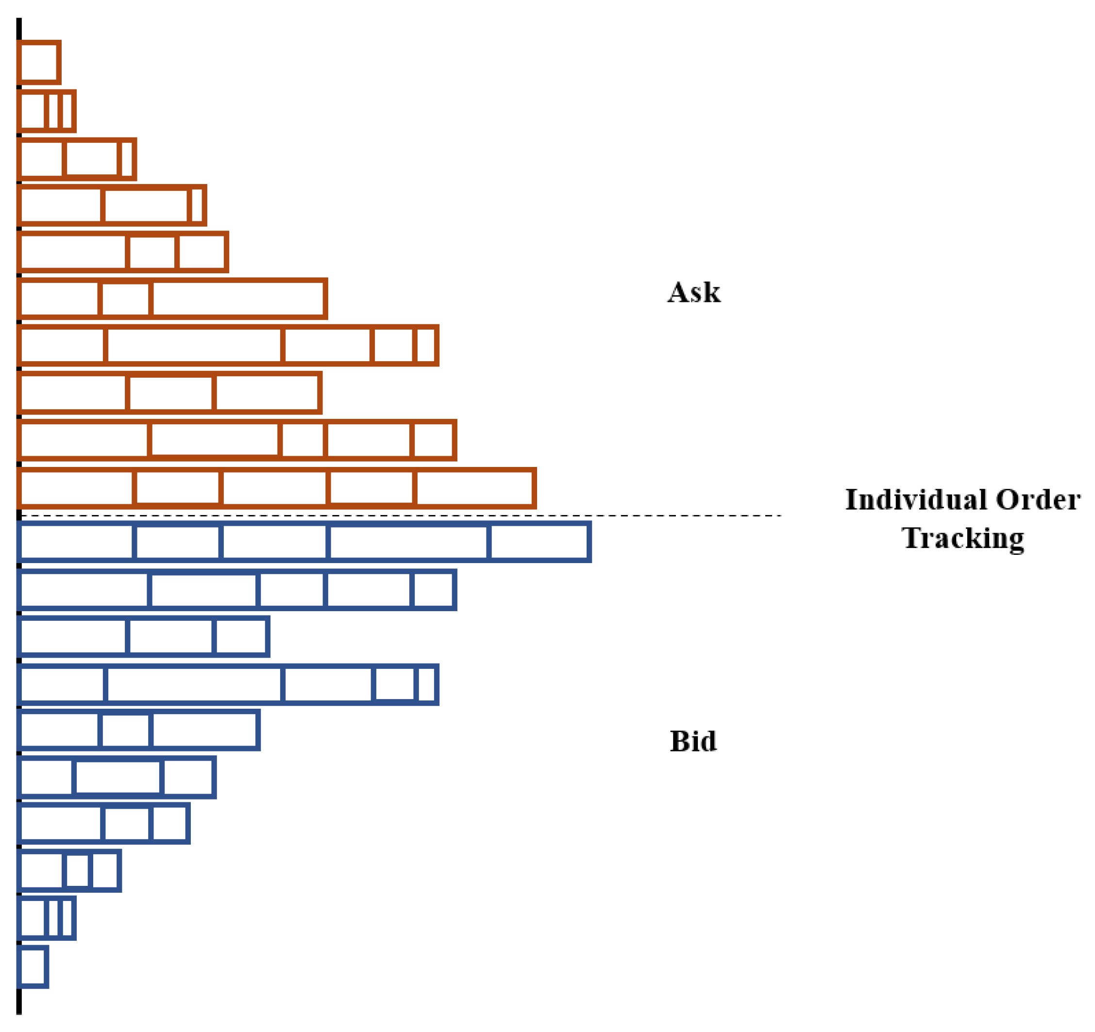
We built an order execution simulation environment utilizing historical level 3 data. Using level 3 data, orders that have been canceled or modified between each time step are known. It is also known exactly which orders have been executed between each time step. These allow us to track individual orders in each price level as shown in Figure 2 which informs us about how many orders with a higher priority are present before the synthetic orders of the agent. In the limit order book mechanism, the priority of orders are determined based on price, followed by time submitted. Without such information, it is necessary to make assumptions about the number of orders having a higher priority as in Li et al. (2022) [10]. As the location of the agent’s synthetic order in the LOB is known, we are able to simulate the market more accurately.
Figure 2.
Depth chart description of the level 3 market simulation. Utilizing the data in (Figure 3) enables the tracking of individual orders.
Figure 2.
Depth chart description of the level 3 market simulation. Utilizing the data in (Figure 3) enables the tracking of individual orders.

At each time step t, the agent can place a market order or limit order. If a market order is placed, it is executed immediately with the best available orders in the opposing book, successively consuming deeper into the opposing book for any remaining quantities. If a limit order is placed, it is first added to the pending orders of the agent. Then, we construct a heap for market execution transactions between time steps and t and for the pending orders of the agent, separately. Both heaps are sorted in a descending order based on the priority of the orders. Subsequently, each pending order is compared with market execution transactions for priority, and every pending order with a higher priority than any of the market execution transactions is executed. It should be noted that when the agent corrects a pending order in the simulation environment, the pending order is first canceled. Then, a new order with the modified price is submitted.
3.3. Validity of Simulation Environment
Even with the most granular market data, it is impossible to completely eliminate market impact in the simulation environment, as accurately simulating the behaviors of all market participants in response to the synthetic orders of the agent is infeasible. One of the most accurate ways to evaluate the magnitude of the discrepancy between the simulation environment and the real market is by executing the exact same on the exact same day in both settings separately. One caveat for this approach is that it can only be done ex post. However, since our algorithm was successfully commercialized and used in the real market during the time period of 1 July 2020–29 December 2021, it is possible to replay those in the simulation environment using historical data. Figure 4 demonstrates the strong positive correlation between the performance of the agent for 4332 in the real market and simulation environments. Each data point represents the performance of the agent for the same on the same day in the real market and in the simulation environment. The performance summary of real market executions can also be found in Table A3.
4. Experimental Results
4.1. Training Set Up
The settings of the environment during training are crucial for the successful learning of the agent. The carefully designed training settings are as follows:
- Side: ask and bid;
- Date range: 1 January 2018–1 January 2020;
- Universe (the full list of stocks is shown in Table A1): Fifty high-trading volume stocks listed on Korea Stock Exchange (KRX);
- Execution time horizon: 165 min–380 min;
- Target volume: 0.05–1% of daily trading volume.
In each episode, a random date is sampled from the date range, and a stock from the universe is selected through weighted random sampling, wherein the weights are determined by the trading volume of each stock for the day. Furthermore, a random execution time horizon and target volume are sampled from their respective ranges. With the sampled execution time horizon, the trading start and trading end times between 9:00 AM and 15:20 PM are also randomly determined. With these specifications, an execution is created for each episode. Then, the agent is trained until convergence with the goal of beating market volume-weighted average price (VWAP) of the same execution time horizon. At the end of the execution time horizon, any remaining shares are submitted as a market order to fulfill the target volume.
4.2. Training Results
In this section, the plots of the training process are presented. In plots (a) and (c) ((b) and (d)) of Figure 5, each data point of the y-axis corresponds to the average performance (win rate) of 200 episodes against the market VWAP.
The average win rate represents the ratio of episodes in which the agent outperformed the market VWAP. The x-axis represents the optimization steps during training. In every plot, PPO-discrete is displayed in red, and PPO-hybrid is displayed in blue. As the training progresses, the average performance converges above the basis point of 0 while the average win rate converges above 50% for both the ask and bid sides, with PPO-discrete converging at a slightly higher point than PPO-hybrid in every case. Convergence of the models above the basis point value of 0 and the 50% win rate is substantial as it demonstrates that the models have, on average, learned to outperform the benchmark for 200 execution generated with a random stock sampled from a 50-stock universe, a random execution time horizon between 165 and 380 minutes, and a random target volume.
4.3. Validation
The settings of the environment during validation is the same as that of the environment during training with one exception. The date range is set to 2 January 2020–31 June 2020 in order to evaluate the efficacy of the trained agent in the out-of-sample data. For each trading day, 50 are created for the agent to execute. Both PPO and DQN are used and compared for the performance and stability. Furthermore, the TWAP strategy with a fixed limit order price is also compared as the baseline strategy. The summarized performance for each model can be found in Table 2. The total field represents the mean performance of the model across all execution . The ask and bid fields represent the mean performance of the model across all ask side and bid side , respectively. It should be noted that all performance values are measured against the market VWAP. As shown in the table, PPO-discrete performed the best, although by a modest margin compared with PPO-hybrid, which is in line with the training results. For both PPO models, it is notable that only two models (ask and bid) were trained to outperform the market VWAP for 12,300 execution that were randomly generated across stocks, an execution time horizon, and a target volume. They also achieved significantly higher performances than the DQN model and baseline TWAP strategy.
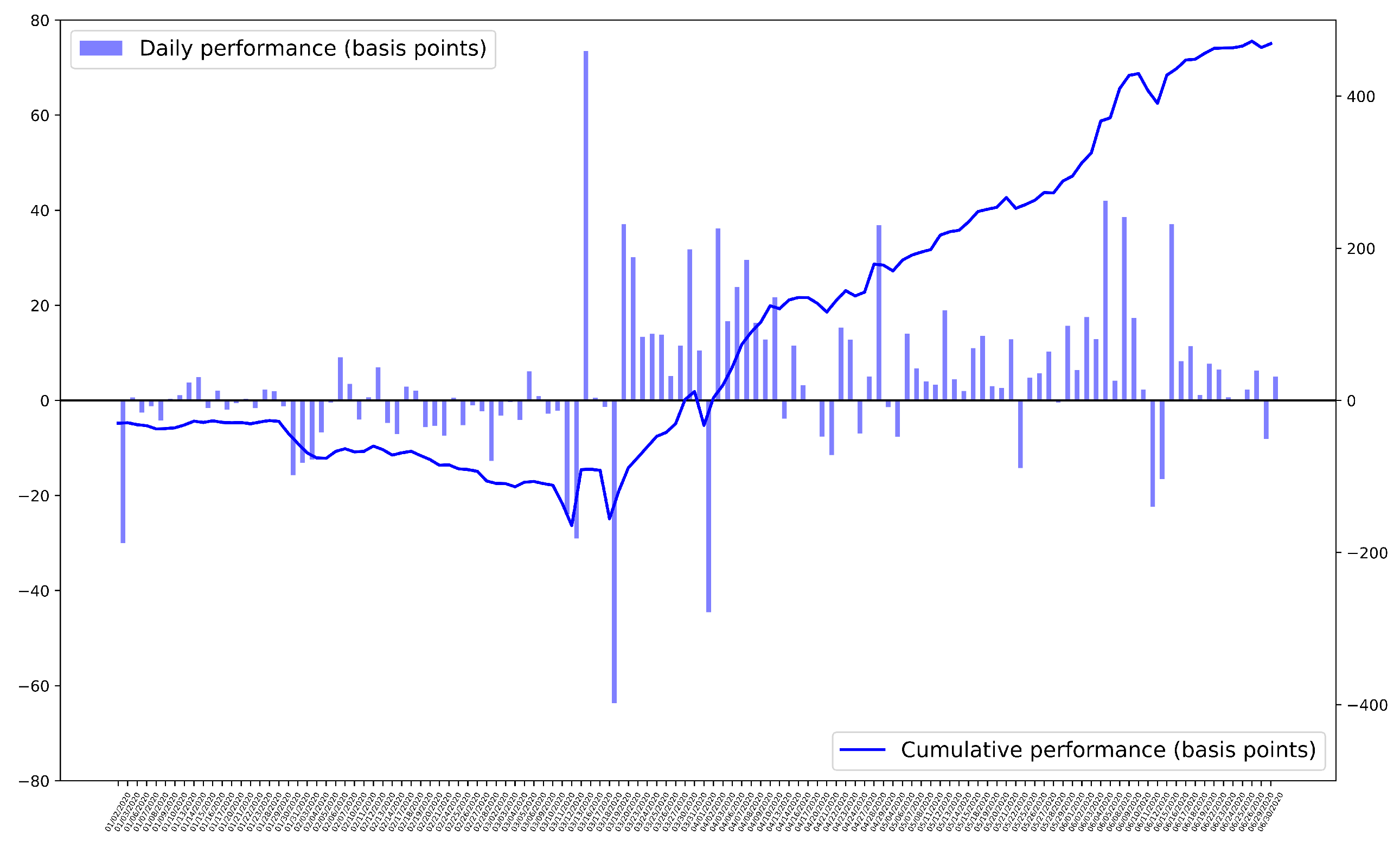
Furthermore, Figure 6 and Figure 7 represent the daily performance of the PPO-discrete model during the validation period. It should be noted that each data point in the bar graphs represents the mean performance of the day across 50 execution . Moreover, the line plots represent the cumulative performance of the model over the validation period. As shown in the figures, for both the ask and bid sides, the final cumulative performance is considerably higher than the basis point of 0. It should also be noted that the y-axis on the left represents the scale of the bar graphs, and the y-axis on the right represents the scale of the line plot.
5. Conclusions
In this study, we addressed the two unresolved issues in applying deep reinforcement learning (DRL) to the optimal trade execution problem. First, we trained a generalized optimal trade execution algorithm by utilizing a widely used reinforcement learning (RL) algorithm, proximal policy optimization (PPO), combined with a long short-term memory (LSTM) network. Moreover, we set up a problem setting in which the DRL agent has the freedom to choose from all possible actions. We presented training results that demonstrate the successful training of the generalized agent, which could handle execution orders for 50 stocks and flexible execution time horizons ranging from 165 min to 380 min with dynamic target volumes. Additionally, the validation result for the 6-month period showed that the trained agent outperformed the market volume-weighted average price (VWAP) benchmark by 3.282 basis points on average for 12,300 execution randomly generated across stocks, an execution time horizon, and target volume. This result is substantial as it demonstrates the efficacy of the generalized model presented in this study. The generalized model is highly practical as it reduces the time spent on training and validation compared with having a model for each stock. Furthermore, Table 1 signifies the practicality of our model and demonstrates that our study is the first to achieve generalization across all three features of stock group size, execution time horizon, and dynamic target volume.
Secondly, we attempted to minimize the discrepancy between the simulation environment and the real market. We built an order execution simulation environment utilizing level 3 market data, which contains information of each order, thus innately allowing for a more precise simulation compared with less granular market data. By also comparing the performances of the trained DRL agent in the simulation environment and in the real market for the same execution on the same day, we further established the validity of the simulation environment. By minimizing this discrepancy, we were able to train the DRL agent accurately, which is demonstrated by successful commercialization in the South Korea stock market for approximately 18 months.
A natural way to extend the presented study would be to apply it to other stock exchanges. However, it would require the same caliber of data. Furthermore, building a simulation environment for each exchange can be demanding and time-consuming. Thus, future work could also extend the study with offline reinforcement learning, where the DRL agent could be trained using historical data without a simulation environment.
Author Contributions
Conceptualization, W.J.B., B.C., S.K. and J.J.; data curation, W.J.B., B.C. and S.K.; formal analysis, W.J.B., B.C. and J.J.; investigation, W.J.B. and B.C.; methodology, W.J.B. and B.C.; project administration, W.J.B. and B.C.; resources, W.J.B. and B.C.; software, W.J.B., B.C., S.K. and J.J.; supervision, W.J.B., B.C., S.K. and J.J.; validation, W.J.B. and B.C.; visualization, W.J.B. and B.C.; writing—original draft, W.J.B. and B.C.; writing—review and editing, W.J.B. and B.C. All authors have read and agreed to the published version of the manuscript.
Funding
This research received no external funding.
Institutional Review Board Statement
Not applicable.
Informed Consent Statement
Not applicable.
Data Availability Statement
Not available.
Conflicts of Interest
The authors declare no conflict of interest.
Appendix A

Table A1.
Stock universe.
| Stock Issue Code |
|---|
| 000060, 000100, 000270, 000660, 000720, 000810, 002790, 003670, 004020, 004990, |
| 005380, 005490, 005830, 005930, 005940, 006400, 006800, 007070, 008560, 008770, |
| 009150, 009830, 010130, 010140, 010620, 010950, 011070, 011170, 011780, 015760, |
| 016360, 017670, 018260, 024110, 028050, 028260, 028670, 029780, 030200, 032640, |
| 241560, 055550, 068270, 033780, 035250, 035420, 066570, 086790, 035720, 307950 |
Table A2.
Hyperparameters for PPO-discrete and PPO-hybrid.
| Hyperparameter | PPO-Discrete | PPO-Hybrid |
|---|---|---|
| Minibatch size | 128 | 128 |
| LSTM size | 128 | 128 |
| Network Dimensions | 256 | 256 |
| Learning rate | ||
| Gradient clip | 1.0 | 1.0 |
| Discount | 0.993 | 0.993 |
| GAE parameter | 0.96 | 0.96 |
| Clipping parameter | 0.1 | 0.1 |
| VF coeff. | 1.0 | 1.0 |
| Entropy coeff. |
Table A3.
Real-market performance summary.
| Year | Count | Avg. Performance (Basis Points) | Win Rate (%) |
|---|---|---|---|
| 2020 | 503 | 11.035 | 54.32 |
| 2021 | 3829 | 1.966 | 51.25 |
| All | 4332 | 3.019 | 51.61 |
References
- Nevmyvaka, Y.; Feng, Y.; Kearns, M. Reinforcement learning for optimized trade execution. In Proceedings of the 23rd International Conference on Machine Learning, Pittsburgh, PA, USA, 25–29 June 2006; pp. 673–680. [Google Scholar]
- Hendricks, D.; Wilcox, D. A reinforcement learning extension to the Almgren-Chriss framework for optimal trade execution. In Proceedings of the 2014 IEEE Conference on Computational Intelligence for Financial Engineering & Economics (CIFEr), London, UK, 27–28 March 2014; pp. 457–464. [Google Scholar]
- Almgren, R.; Chriss, N. Optimal execution of portfolio transactions. J. Risk 2001, 3, 5–40. [Google Scholar] [CrossRef] [Green Version]
- Mnih, V.; Kavukcuoglu, K.; Silver, D.; Graves, A.; Antonoglou, I.; Wierstra, D.; Riedmiller, M. Playing atari with deep reinforcement learning. arXiv 2013, arXiv:1312.5602. [Google Scholar]
- Dabérius, K.; Granat, E.; Karlsson, P. Deep Execution-Value and Policy Based Reinforcement Learning for Trading and Beating Market Benchmarks. 2019. Available online: https://ssrn.com/abstract=3374766 (accessed on 21 April 2019).
- Ye, Z.; Deng, W.; Zhou, S.; Xu, Y.; Guan, J. Optimal trade execution based on deep deterministic policy gradient. In Proceedings of the Database Systems for Advanced Applications: 25th International Conference, DASFAA 2020, Jeju, Republic of Korea, 24–27 September 2020; Springer: Berlin/Heidelberg, Germany, 2020; pp. 638–654. [Google Scholar]
- Ning, B.; Lin, F.H.T.; Jaimungal, S. Double deep q-learning for optimal execution. Appl. Math. Financ. 2021, 28, 361–380. [Google Scholar] [CrossRef]
- Lin, S.; Beling, P.A. An End-to-End Optimal Trade Execution Framework based on Proximal Policy Optimization. In Proceedings of the Twenty-Ninth International Joint Conference on Artificial Intelligence, Yokohama, Japan, 11–17 July 2020; pp. 4548–4554. [Google Scholar]
- Shen, Y.; Huang, R.; Yan, C.; Obermayer, K. Risk-averse reinforcement learning for algorithmic trading. In Proceedings of the 2014 IEEE Conference on Computational Intelligence for Financial Engineering & Economics (CIFEr), London, UK, 27–28 March 2014; pp. 391–398. [Google Scholar]
- Li, X.; Wu, P.; Zou, C.; Li, Q. Hierarchical Deep Reinforcement Learning for VWAP Strategy Optimization. arXiv 2022, arXiv:2212.14670. [Google Scholar]
- Kyle, A.S.; Obizhaeva, A.A. The Market Impact Puzzle. 2018. Available online: https://ssrn.com/abstract=3124502 (accessed on 4 February 2018).
- Bertsimas, D.; Lo, A.W. Optimal control of execution costs. J. Financ. Mark. 1998, 1, 1–50. [Google Scholar] [CrossRef]
- Watkins, C.J.; Dayan, P. Q-learning. Mach. Learn. 1992, 8, 279–292. [Google Scholar] [CrossRef]
- Mnih, V.; Kavukcuoglu, K.; Silver, D.; Rusu, A.A.; Veness, J.; Bellemare, M.G.; Graves, A.; Riedmiller, M.; Fidjeland, A.K.; Ostrovski, G.; et al. Human-level control through deep reinforcement learning. Nature 2015, 518, 529–533. [Google Scholar] [CrossRef] [PubMed]
- Van Hasselt, H.; Guez, A.; Silver, D. Deep reinforcement learning with double q-learning. In Proceedings of the AAAI Conference on Artificial Intelligence, Phoenix, AZ, USA, 12–17 February 2016; Volume 30. [Google Scholar]
- Karpe, M.; Fang, J.; Ma, Z.; Wang, C. Multi-agent reinforcement learning in a realistic limit order book market simulation. In Proceedings of the First ACM International Conference on AI in Finance, New York, NY, USA, 15–16 October 2020; pp. 1–7. [Google Scholar]
- Lillicrap, T.P.; Hunt, J.J.; Pritzel, A.; Heess, N.; Erez, T.; Tassa, Y.; Silver, D.; Wierstra, D. Continuous control with deep reinforcement learning. arXiv 2015, arXiv:1509.02971. [Google Scholar]
- Schulman, J.; Wolski, F.; Dhariwal, P.; Radford, A.; Klimov, O. Proximal policy optimization algorithms. arXiv 2017, arXiv:1707.06347. [Google Scholar]
- Hochreiter, S.; Schmidhuber, J. Long short-term memory. Neural Comput. 1997, 9, 1735–1780. [Google Scholar] [CrossRef] [PubMed]
- Berkowitz, S.A.; Logue, D.E.; Noser Jr, E.A. The total cost of transactions on the NYSE. J. Financ. 1988, 43, 97–112. [Google Scholar] [CrossRef]
- Kakade, S.M.; Kearns, M.; Mansour, Y.; Ortiz, L.E. Competitive algorithms for VWAP and limit order trading. In Proceedings of the 5th ACM Conference on Electronic Commerce, New York, NY, USA, 17–20 May 2004; pp. 189–198. [Google Scholar]
- Wang, Z.; Schaul, T.; Hessel, M.; Hasselt, H.; Lanctot, M.; Freitas, N. Dueling network architectures for deep reinforcement learning. In Proceedings of the International Conference on Machine Learning, Anaheim, CA, USA, 18–20 December 2016; pp. 1995–2003. [Google Scholar]
- Sutton, R.S.; Barto, A.G. Reinforcement Learning: An Introduction; MIT Press: Cambridge, MA, USA, 2018. [Google Scholar]
- Pardo, F.d.M.; Auth, C.; Dascalu, F. A Modular Framework for Reinforcement Learning Optimal Execution. arXiv 2022, arXiv:2208.06244. [Google Scholar]
Figure 1.
The overall architecture of the PPO model for optimal trade execution.

Figure 3.
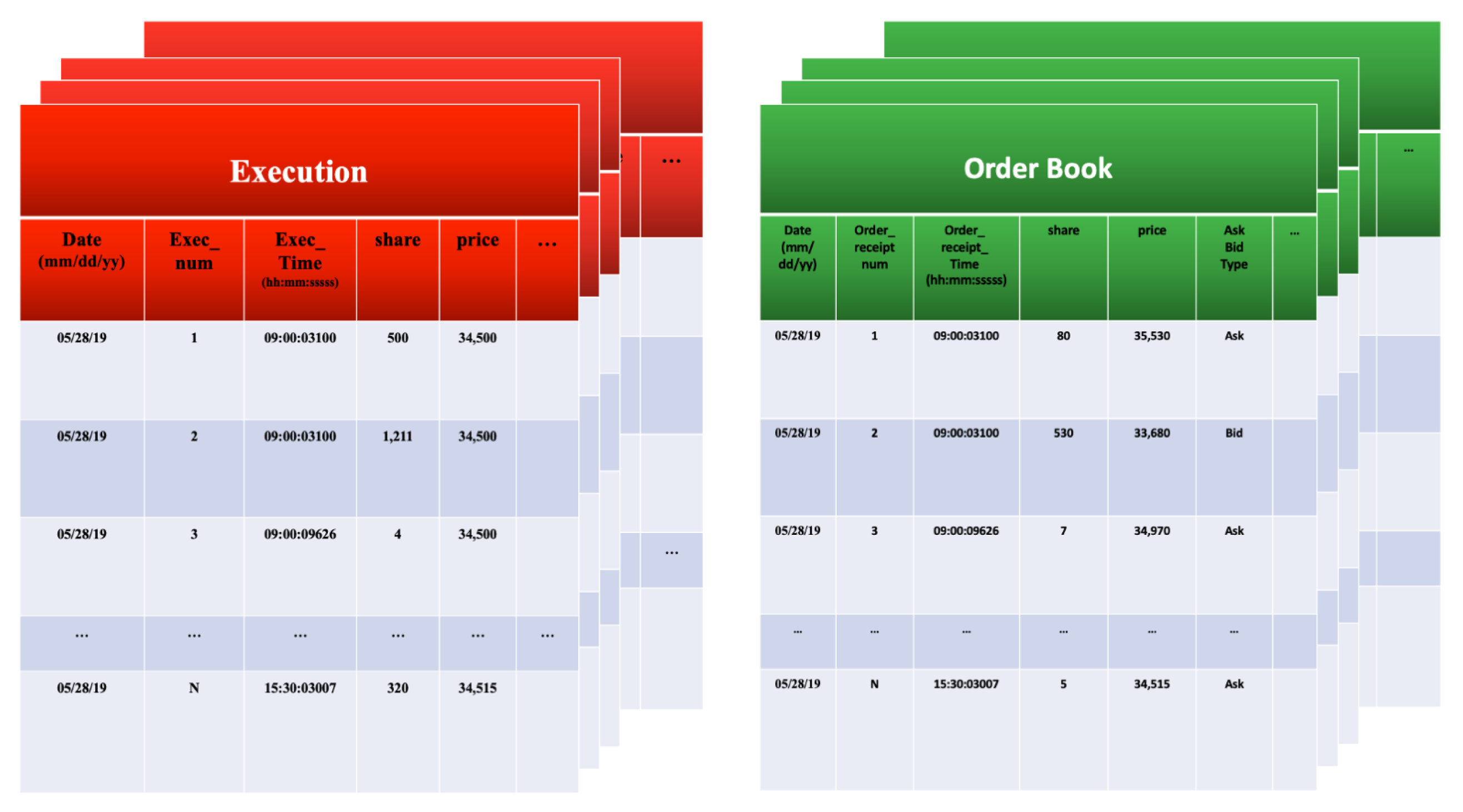
Sample date (28 May 2019) description of execution data (Left) and order book data (Right) for the level 3 market simulation environment.
Figure 3.
Sample date (28 May 2019) description of execution data (Left) and order book data (Right) for the level 3 market simulation environment.

Figure 4.
Real market vs. simulation environment.

Figure 5.
PPO training plots. (a) Ask side performance, (b) ask side win rate, (c) bid side performance, (d) bid side win rate.
Figure 5.
PPO training plots. (a) Ask side performance, (b) ask side win rate, (c) bid side performance, (d) bid side win rate.

Figure 6.
Daily average performance—Ask.

Figure 7.
Daily average performance—Bid.

Table 1.
Existing studies of RL for optimal trade execution.
| Author | Stock Group Size | Execution Time Horizon | Dynamic Target Volume |
|---|---|---|---|
| Nevmyvaka et al. [1] | 3 | 2–8 min | No |
| Hendricks and Wilcox [2] | 166 | 20–60 min | No |
| Shen et al. [9] | 1 | 10 min | No |
| Ning et al. [7] | 9 | 60 min | No |
| Ye et al. [6] | 3 | 2 min | No |
| Lin and Beling [8] | 14 | 1 min | No |
| Li et al. [10] | 8 | 240 min | No |
| Our study | 50 | 165–380 min | Yes |
Table 2.
Validation performance comparison.
| Algorithm | Total (Basis Points) | Ask (Basis Points) | Bid (Basis Points) |
|---|---|---|---|
| PPO-Discrete | 3.282 | 2.719 | 3.845 |
| PPO-Hybrid | 3.114 | 2.604 | 3.623 |
| DQN | −3.752 | −4.351 | −3.153 |
| TWAP Strategy | −10.420 | −9.824 | −11.015 |
Disclaimer/Publisher’s Note: The statements, opinions and data contained in all publications are solely those of the individual author(s) and contributor(s) and not of MDPI and/or the editor(s). MDPI and/or the editor(s) disclaim responsibility for any injury to people or property resulting from any ideas, methods, instructions or products referred to in the content. |
© 2023 by the authors. Licensee MDPI, Basel, Switzerland. This article is an open access article distributed under the terms and conditions of the Creative Commons Attribution (CC BY) license (https://creativecommons.org/licenses/by/4.0/).
Share and Cite
MDPI and ACS Style
Byun, W.J.; Choi, B.; Kim, S.; Jo, J. Practical Application of Deep Reinforcement Learning to Optimal Trade Execution. FinTech 2023, 2, 414-429. https://doi.org/10.3390/fintech2030023
AMA Style
Byun WJ, Choi B, Kim S, Jo J. Practical Application of Deep Reinforcement Learning to Optimal Trade Execution. FinTech. 2023; 2(3):414-429. https://doi.org/10.3390/fintech2030023
Chicago/Turabian StyleByun, Woo Jae, Bumkyu Choi, Seongmin Kim, and Joohyun Jo. 2023. "Practical Application of Deep Reinforcement Learning to Optimal Trade Execution" FinTech 2, no. 3: 414-429. https://doi.org/10.3390/fintech2030023