
Enhancing Energy Efficiency in IoT-NDN via Parameter Optimization

Insitute of Telematics, University of Lübeck, 23562 Lübeck, Germany
*
Author to whom correspondence should be addressed.
Future Internet 2024, 16(2), 61; https://doi.org/10.3390/fi16020061
Submission received: 12 January 2024
/
Revised: 9 February 2024
/
Accepted: 12 February 2024
/
Published: 16 February 2024
(This article belongs to the Special Issue Featured Papers in the Section Internet of Things)
Abstract
:The IoT encompasses objects, sensors, and everyday items not typically considered computers. IoT devices are subject to severe energy, memory, and computation power constraints. Employing NDN for the IoT is a recent approach to accommodate these issues. To gain a deeper insight into how different network parameters affect energy consumption, analyzing a range of parameters using hyperparameter optimization seems reasonable. The experiments from this work’s ndnSIM-based hyperparameter setup indicate that the data packet size has the most significant impact on energy consumption, followed by the caching scheme, caching strategy, and finally, the forwarding strategy. The energy footprint of these parameters is orders of magnitude apart. Surprisingly, the packet request sequence influences the caching parameters’ energy footprint more than the graph size and topology. Regarding energy consumption, the results indicate that data compression may be more relevant than expected, and caching may be more significant than the forwarding strategy. The framework for ndnSIM developed in this work can be used to simulate NDN networks more efficiently. Furthermore, the work presents a valuable basis for further research on the effect of specific parameter combinations not examined before.
1. Introduction
The concept of the Internet of Things (IoT) relates to the networking of devices that go beyond traditional computers, including sensors and everyday objects. The vision of IoT is to interconnect diverse entities, enabled by the proliferation of compact and cost-effective embedded devices [1]. This “IoT revolution”, as described by [2], spans the realms of technology, policy, and engineering, with a notable presence in popular media. Notable consumer applications encompass Internet-connected appliances, energy management systems, components for home automation, as well as wearable fitness and health trackers.
Clearly, the Internet of Things stands out as one of the primary topics in networking at present. Traditionally, IPv6 has served as a network protocol for connecting IoT devices. However, Information-Centric Networking, and more specifically Named Data Networking (NDN), have drawn significant attention in recent research on future Internet technologies. NDN constitutes a novel networking paradigm, representing an evolution of the traditional IP architecture [3]. Numerous authors have described it as a promising technology [4,5,6], a key enabling paradigm for IoT [7], and some have even referred to it as revolutionary [8]. The enthusiasm for NDN is driven by its ability to address numerous classical TCP/IP-related issues such as location dependence, scalability, node mobility, intermittent connectivity, and network overhead, as documented in [9].
The motivation for the NDN protocol stems from the limitations of the existing host-centric paradigm in today’s Internet. There is a clear need for an alternative approach that shifts the focus from the location of data to the data itself. Users are increasingly interested in accessing data, while possibly being unaware of its location. NDN addresses this shift while also enhancing security, privacy, and efficient data retrieval. By enabling caching of information closer to consumers, it reduces network overhead and supports the growing number of devices and mobility requirements in the modern network landscape.
Given the inherent constraints of IoT devices in terms of energy, memory, and computational resources [10], optimizing energy consumption in communication is a critical aspect, which is the primary focus of this work. For many IoT devices, network communication accounts for a significant portion of their energy consumption. Therefore, reducing energy consumption through communication can significantly decrease a device’s overall energy footprint.
This work finds the energetically best parameter combinations in a set of given parameters using hyperparameter optimization. The primary objective is to investigate the impact of network parameters, such as network size, topology, packet size, and the number of sent packets, on energy consumption within the network. Breaking down networks into a set of distinct parameters enables a precise analysis of various factors that influence energy consumption. However, for most parameters, the number of potential combinations increases exponentially. This presents a substantial challenge as the goal is to discover the optimal global energy consumption within all possible combinations.
To address this issue, the problem is reframed as a hyperparameter optimization problem, a concept derived from machine learning. A fundamental algorithm employed in this field is grid search. This algorithm conducts an exhaustive search of all parameter combinations, which, in turn, leads to an exponential increase in the number of iterations. Consequently, it becomes imperative to minimize the number of parameters and their value ranges.
In addition, this work also endeavors to contribute to the advancement of NDN research through the development of an innovative framework within ndnSIM. This framework offers enhanced efficiency in simulating NDN networks, providing researchers with a valuable tool for more accurate and resource-effective evaluations of NDN-based IoT network configurations. The development of such a framework not only streamlines the simulation process but also holds the potential to accelerate progress in NDN network optimization, ultimately benefiting the broader IoT ecosystem. The developed framework simplifies parameter configuration within networks and serves as a foundational tool for conducting network experiments. The contributions can be summarized as follows:
- Simple Parameter Definition for Diverse Experiments: The framework allows a declarative definition of parameters, rather than an imperative approach, as would be necessary when using plain ndnSIM: Instead of having to configure all the necessary networking objects manually, users can simply define a set of desired parameter values. This facilitates the conduction of a wide range of IoT-NDN-related experiments considerably.
- Identification of Optimal Parameter Combinations: It enables the identification of the most energy-efficient network parameter combinations using the hyperparameter optimization algorithm grid search.
- Automated Visualization of Results: The framework automates the visualization of experiment results, enhancing the clarity and comprehension of outcomes.
- Integration of Caching Schemes and Strategies: It incorporates new caching strategies and schemes into the framework and allows for straightforward extensions to accommodate additional strategies and schemes in the future.
- Automatic Graph Generation: The framework streamlines data representation by automatically generating graphs directly from network parameters like the topology or graph size.
The remainder of this paper is organized into the following sections: Section 2 introduces related work on fundamental concepts, IoT-NDN and ndnSIM. Moving on, Section 3 outlines the essentials of the NDN protocol, including an exploration of its various packet types and data structures. In Section 4, we explore the architecture of the framework proposed in this work, providing insights into the key parameters that can be configured using this framework. Moving on to Section 5, we introduce the reader to ndnSIM, the chosen simulator for implementing the previously discussed parameters. Here, we outline the framework’s structure and provide a detailed account of how we implemented crucial parameters within the simulator. Section 6 provides a detailed explanation of our approach to analyzing network-related parameters for IoT-NDN. The primary objective is to identify optimal parameter combinations for minimizing energy consumption. Finally, in Section 7, we conclude the paper by summarizing our key findings and engaging in a discussion regarding energy efficiency in IoT-NDN through parameter optimization and possible future applications.
2. Related Work
This section highlights the importance of the IoT-NDN research field and identifies several pertinent articles. It also introduces research that employs ndnSIM to evaluate application fields related to NDN.
A primary focus in reviewing IoT-NDN networks is on energy consumption. Numerous studies provide insights into various aspects of IoT-NDN. In the following, we will present papers related to the fundamental concepts of IoT-NDN, energy efficiency in real-world IoT-NDN environments, and performance analysis using ndnSIM.
Fundamental Concepts: The study by [10] addresses challenges in IoT and proposes an NDN-based IoT system architecture, establishing foundational concepts in this field. NDN, initially designed to enhance the Internet’s communication structure, is now extended to wireless networks such as ad-hoc and wireless sensor networks [11,12,13,14]. In these scenarios, NDN offers numerous benefits, including mobility support, low-cost configuration, delay tolerance, and opportunistic networking. Furthermore, integrating NDN into IoT is argued to enhance system efficiency, flexibility, and robustness [15].
Real-World IoT-NDN and Energy Efficiency: Here, we explore research within the realm of Named Data Networking (NDN), with a particular focus on energy efficiency achieved through caching strategies. The work conducted by [9,14,16] collectively examines the influence of caching parameters on IoT energy consumption using NDN. Specifically, Ref. [14] provides a detailed comparison between the energy efficiencies of NDN and IPv6 within IoT nodes, investigating a variety of forwarding strategies and caching scenarios. These articles delve into practical network implementations, highlighting the role of caching strategies, data production, and energy-saving measures. However, they do not fully explore the various parameters and combinations that could significantly impact the outcomes of energy consumption studies.
Unfortunately, this comprehensive approach to analyzing parameter combinations related to energy efficiency in IoT-NDN has not been addressed in the works mentioned above. Our contribution lies in our thorough consideration of all relevant parameter combinations to optimize energy consumption in this field, providing practical steps for researchers to enhance energy efficiency in IoT-NDN deployments.
Performance Analysis using ndnSIM: Our research paper examines how different caching methods and network designs impact the efficiency of Named Data Networking (NDN), focussing on aspects such as server workload, data access rates, and the performance of various caching rules like FIFO, LRU, and Universal Caching, as explored in studies [17,18]. It also discusses the optimization of caching for energy savings in vehicular networks through ndnSIM [19].
Refs. [20,21] explore the deployment of Named Data Networking (NDN) in Mobile Ad Hoc Networks (MANETs) and the utilization of simulation tools like ndnSIM for research purposes. Through our extension of ndnSIM, we have enhanced the efficiency and flexibility of NDN within MANET environments. This advancement supports and simplifies conducting experiments using ndnSIM for MANET-related research.
Additionally, we build upon the fundamental analysis of ndnSIM’s development and its role in NDN research as presented in [22]. While [21,23] utilize ndnSIM for experiments described in these articles, they do not explore the vast array of combinations that could be tested during experiments due to the complexity and the time-consuming nature of such configurations in ndnSIM simulations. Our work extends ndnSIM’s capabilities by incorporating novel features such as optimal parameter combinations and presenting simple steps to build, test, and evaluate experiments, which simplifies the presentation of all experimental results. Furthermore, the framework presented in this article automates experiments using ndnSIM, a capability not currently considered or present in previously mentioned articles related to our work.
Our article introduces a unique framework for conducting IoT-NDN experiments with ndnSIM, making research more straightforward and effective. This framework allows for easy setup through a declarative approach to defining experiment parameters, identifies the most energy-efficient network configurations using methods like grid search optimization, identifies the optimal parameter combinations, and enhances result interpretation through automated visualizations and graph generation, showcasing a comprehensive suite of features not found in previous studies.
3. Basics
This section introduces the basics of the NDN protocol, its different packet types, and data structures. We then address NDN specifically for the Internet of Things, as well as the challenges this entails.
3.1. Named Data Networking
Named Data Networking (NDN) is a novel network technology developed on top of Information-Centric Networking (ICN) [24]. NDN was first presented in [3] in 2014.
The Internet Protocol (IP) is based on the notion that every host has a globally unique address, known as an IP address. The prefix of this address gives away a host’s approximate location, enabling routers to forward packets to the correct subnetworks.
In contrast, NDN does not have such a concept of a host-specific address: Instead, every packet has a name unique for the network. This name is independent of the host’s location. Thus, with NDN, the focus shifts from location-centric to data-centric networking.
In an NDN network, a consumer is interested in data from the network produced by one or more producers. To express interest in some data, a consumer can send an Interest packet, which is uniquely identified by its name. Network nodes between the consumer and some producer forward the packet until a producer that retains the data has been found. The producer then returns a Data packet with the same name and the corresponding payload.
The primary data structures in NDN are the Content Store, Pending Interest Table, Forwarding Information Base, and the forwarding strategy. The Content Store (CS) is an in-network cache, allowing each node to make a local copy of a Data packet if appropriate. If a node cannot find a packet name in its CS, the Pending Interest Table (PIT) stores all the pending Interests that a node has forwarded to other nodes. The Forwarding Information Base (FIB) keeps track of the name prefixes of incoming Interest packets. The forwarding strategy fetches the longest matching prefix from the FIB and decides when, where, or even whether to forward an Interest packet. For a more detailed review of these data structures, one may refer to [3].
3.2. Named Data Networking in the Internet of Things
The Internet of Things (IoT) is a term first coined by Kevin Ashton in 1999. It generally refers to scenarios where network connectivity and computing capability extends to objects, sensors, and everyday items not normally considered computers, allowing these devices to generate, exchange, and consume data with minimal human intervention [2].
Thus, the IoT refers explicitly to devices with severe resource limitations, such as smartwatches, smart home devices, or traffic control devices. Particularly, such devices face memory, energy, and computation power restrictions [10]. The available resources are orders of magnitude smaller than for classical computers like desktop PCs or laptops.
If we want to use the NDN protocol in IoT scenarios (called IoT-NDN), NDN faces specific constraints, specifically the packet length, data aggregation, and packet naming [25] problems. In the original definition of the NDN protocol [3], the packet length is not fixed but variable. However, in the IoT, the MTU limiting the maximum packet size is often quite small, so the packet length has to be restricted. Unfortunately, NDN does not provide a fragmentation mechanism like IP. Data aggregation refers to the problem that requesting a series of packets at once, e.g., with suffixes named 1 through n, is impossible. For each Interest packet in the series, the consumer has to signify the packets it has already received in the so-called exclude parameter. This may create major overhead if many names are included in this exclude parameter [10]. Finally, naming can be problematic since NDN names are typically intended to be human-readable. If such names are used, and the names are very long, the name itself can add dozens of bytes of overhead. While this problem can be compensated by abbreviating names, it would be at the cost of readability.
4. Framework Architecture
This section concentrates on the architecture of the presented framework. We demonstrate the primary parameters configurable using the framework, followed by an explanation of how to measure energy consumption in an IoT setting. Finally, the parameter setup is embedded into a hyperparameter optimization setting, which serves as an automated tool to search for the best parameter combinations.
4.1. Modeling the Parameters
The modeling parameters originally stem from [26]. Only the key parameters will be presented in detail here. For a more in-depth review, one may refer to said thesis. An overview of the parameters is shown in Figure 1, where each parameter, its category, and its possible values are demonstrated. The categories marked with blue are only applicable to NDN networks, the white ones to arbitrary networks, and the text below denotes the actual parameters and the values they can assume. Each parameter is addressed abstractly and independently of the implementation so that the ideas can be applied both to simulated and real networks.
4.1.1. Graph Size
Graphs are a valuable tool for modeling networks mathematically. Since network connections are typically bidirectional, the graphs are assumed to be undirected in this paper. The graph size describes how many nodes are part of the network. Here, we allow an arbitrary integer as the number of nodes for the network since this allows for the creation of any kind of network desired.
4.1.2. Graph Topology
A graph topology describes a category of graph shapes with certain common characteristics. In this paper, we focus on relatively simple topologies, namely random, complete, star, connected stars, and grid. It is key that the graph is connected—otherwise, each connected component would constitute a separate graph that could be analyzed by itself.
A random graph is generated here by iterating all pairs of nodes: With a fixed probability p, an edge between each pair is created. Thus, given graph and probability for event X, , where . Therefore, it is not guaranteed that the generated graph is connected. However, by creating a series of s random graphs, the probability that the graph is connected approaches 1 with .
A complete graph is a graph in which each pair of nodes is mutually connected. Thus, each node can reach every other node in just one hop.
A star graph has a designated node called center node to which all other nodes are connected. The non-center nodes are not connected to each other. Communication always has to go through the center node, making it prone to being a bottleneck in the network.
The connected-stars topology consists of pairwise disjunctive star graphs, each of size q, whose center nodes are connected with fixed probability p. We assume the graph size n to be a multiple of q. Let C be the set of center nodes, then .
Finally, in the grid topology, the graph is assumed to be a square shape: Each internal node has four neighbors, the edge nodes have three, and the corner nodes have two. Restricting the shape to squares only means that the graph size n must be for some .
4.1.3. Caching Strategy
The caching strategy, or cache replacement strategy, decides what element should be evicted when the Content Store of a node is full. As illustrated in Section 3.2, the IoT is subject to severe resource constraints, so using simple data structures and low-complexity algorithms for caching is desirable. The presented caching strategies are Random, LRU, LFU, LRFU, FWF, and FIFO.
Random is a trivial strategy that uniformly draws a random number from the set and evicts the element with that index. This makes the strategy computationally inexpensive.
LRU (Least Recently Used) keeps track of the last time each element has been requested. It evicts the element that has not been requested for the longest time by maintaining a timestamp that is incremented for every element access. The current timestamp is assigned to the requested element, and the element with the smallest assigned timestamp value is removed.
LFU (Least Frequently Used) is similar to LRU in that it considers the recent popularity of an element but instead maintains a counter that keeps track of the number of accesses for each element. The strategy is good at recognizing data that becomes popular through many recent accesses.
LRFU (Least Recently/Frequently Used) [27] can be considered in between the extremes of LRU and LFU: While LRU gives weight only to the most recent access of an element, LFU gives equal weight to all accesses of an element (the frequency). LRFU, on the other hand, compromises between these two ideas by giving more weight to more recent accesses and less weight to less recent ones. This can be controlled by the weighing function . The parameter ranges from 0 to 1 and allows a trade-off between recency and frequency. As approaches 0, LRFU is more frequency-inclined, whereas approaching 1 leads to a more recency-based policy. This function is used to compute the so-called CRF (Combined Recency and Frequency) value. Given the current time T, the element b to consider and its k reference times , the CRF value can be computed as follows:
FWF (Flush When Full) deletes all elements in the Content Store when it is full and inserts the new element after that.
FIFO (First-In First-Out) maintains a queue of elements for the Content Store. The queue first removes the element that was added first to the Content Store. While this strategy is similar to LRU, FIFO does not keep a recency counter for each element. So, accessing an element already present in the Content Store does not affect the position in the queue.
4.1.4. Caching Scheme
A caching scheme is an algorithm that decides whether an incoming element should be added to the Content Store in the first place. Typically, caching algorithms (e.g., in CPU caches) cache every element, but in networking, this is not necessarily desirable. For example, assume a Data packet has to travel n nodes from the producer to the consumer. If that packet is cached on every node, it will be present in all n Content Stores in between. Hence, there is a lot of redundant data on many neighboring nodes. It is, however, often more reasonable not to cache every incoming element, leaving space for more different packets on neighboring nodes. An example of such a scheme is the probabilistic scheme, but for comparison, one can also use the schemes CEE and no caching, which will be discussed next.
CEE (Caching Everything Everywhere) is a naive scheme that always caches every element. While it minimizes the number of hops to access an element, there is less space for other elements and less data diversity.
While no caching neglects one key feature of NDN and cannot be expected to lead to lower energy consumption, it can be useful to use it as a baseline to compare other schemes against.
Probabilistic caching is a simple algorithm that uses a fixed caching probability across the network: Given a probability for the entire network, each Content Store will cache an incoming element with probability p. This has the major advantage that no extraneous communication is required to exchange caching information between nodes, which would increase the energy consumption. When using this scheme, it can be expected that data in the network will be distributed better than with CEE.
4.1.5. Forwarding Strategy
The forwarding strategy decides when and where to forward a packet. Factors like the priority of an Interest or load balancing may play a role here. The strategies presented here are all implemented in ndnSIM: best-route, access, ASF, multicast, random, and self-learning. The following information is based on [28].
- The best-route strategy forwards to the upstream node with the lowest cost. When a consumer transmits an Interest again, the strategy forwards the packet to the lowest-cost node that was previously not used.
- The access strategy sends the first Interest packet to all adjacent upstream nodes. When the corresponding Data packet returns, the last working upstream node is stored for the prefix and will be used for all subsequent Interests.
- The ASF (Adaptive Smoothed RTT-based Forwarding) strategy uses hyperbolic routing as a strategy: By embedding the network topology into the hyperbolic plane, a greedy geometric routing algorithm never gets stuck at local minima. Thus, it can be avoided that a forwarder has to keep next-hop routes to all destinations in the network in its FIB.
- The multicast strategy forwards an Interest packet to all upstream neighbors.
- The random strategy randomly selects an upstream node to forward a packet to.
- The self-learning strategy first broadcasts Interests to “learn” a path towards data, and then unicasts the following Interests across the same learned path.
4.1.6. Consumer Sequence Type
A consumer sequence type is a scheme by which different packet names are generated. We assume that all requested packets have the same prefix and only the suffixes of the requests differ, e.g., example/packet0, example/packet1, etc. In the following, only the suffixes denote the packet names for the different sequence types. In particular, these sequence types are incremental, repetitive, simple random, and linear random. They have been taken from [26].
Incremental is of the form , where p is the number of repetitions of the sequence and is the maximum sequence number. The type can be used to model packets requested in a regular pattern.
Repetitive has the form , where p is the number of repetitions per element and k is the number of repetitions of the entire sequence. This type can be used to simulate a network with many repeated requests.
Simple random selects a uniformly random element from and can be used to model packet names with no discernible pattern.
Linear random also selects a random element from , but the distribution is not uniform: Instead, assuming , the probability for suffix is . It can easily be seen that . Certain packets are assumed to be more relevant to a consumer than others here.
4.1.7. Other Parameters
The parameters presented thus far are the focus of this work, but others are shown in Figure 1, which will be sketched next. Since we do not consider these parameters central, they will only be summarized. Again, one may refer to [26] for more details.
- The energy capacity refers to the initial energy of a node, measured in joule.
- The energy consumption refers to the states of a Wi-Fi connection between a pair of nodes, namely RX (receive), TX (transmit), IDLE, and SLEEP. It is measured in ampere.
- Besides the types of different packets to be sent (sequence types), one can also consider different packet sizes and number of packets.
- The observation length is the length that we consider the communication in a network, in our case, the length of the network simulation.
- The number of consumers and producers can largely affect the amount of communication in the network: The more producers there are, the smaller we expect the average paths to be between consumers and producers. Furthermore, one may have overlapping consumers and producers, meaning one node fulfills both roles.
- The Content Store size is the number of packets that can be stored on a node.
4.2. Energy Consumption in IoT-NDN
It has already been stated that IoT devices are often very restricted in terms of energy capacity, memory, and computation power. In this paper, we want to focus specifically on reducing energy consumption. For that matter, we assume that most of the network’s energy is consumed by network communication, not actual CPU computation. Ref. [29] argues that radio interfaces cause up to 50% of smartphones’ energy consumption during typical usage. The canonical unit to measure energy is the joule (J), where [30]. The voltage (V) should be specified for a device, the electric current (A) depends on the state in which the device currently is, and the time (s) can be measured as the time span that the device takes on a certain state. These states refer to the different Wi-Fi states like idle or transmission. The total energy consumption per device is computed by summing up the energy consumption per state.
More formally, let be a device’s voltage, and the electric currents for the n different states. Let be the n time spans that the corresponding states last, where corresponds to and T is the total runtime of the experiment. Then the total energy consumed by a device can be computed like this:
To evaluate the overall performance of a network, we compute the average energy consumption per node , where n is the graph size and is the energy consumption of the i-th device.
4.3. Hyperparameter Optimization
Since analyzing the multitude of parameters from Section 4.1 manually can be difficult and time-consuming, it may come to mind to automate the parameter selection process. In this paper, we do this using a machine learning concept called hyperparameter optimization. While the training parameters of a machine learning model are modified during the training phase, the hyperparameters are specified prior to the learning phase. The goal is to find a set of hyperparameters that generates the best model according to some heuristic [31]. For a more formal definition of hyperparameter optimization, one may refer to [32].
Parameter optimization in IoT-NDN and hyperparameter optimization are similar because they both search for a set of parameters that optimizes some predefined objective function. In the case of machine learning, the objective function is evaluated using a validation data set. In contrast, here we evaluate the performance—namely the energy consumption—by actually performing the simulation on the networks.
The grid search algorithm is of particular interest due to its simplicity. As described in [33], it performs a complete search on a given subset of the hyperparameter space of the training algorithm. In our case, we search on a predefined subset of the network parameters. Grid search is subject to the curse of dimensionality since the number of combinations grows exponentially with every added parameter [31]. Hence, using the algorithm for many parameters or with a large search space is impractical. This is why we keep our test scenarios relatively small in this paper regarding the number of variable parameters and the values per parameter.
5. Implementation
In the Implementation section, we introduce ndnSIM, the simulator used for the implementation of the parameters shown before. The structure of the implemented framework is sketched, followed by a more detailed illustration of how we realized the critical parameters in the simulator. For brevity, not all parameters from Section 4.1 are reiterated. After that, we address how to use the energy model in ns-3, and finally, the implementation of grid search, the hyperparameter optimization algorithm of choice, is addressed.
5.1. ndnSIM—An ns-3-Based Simulator
ndnSIM (Named Data Networking simulator) is an open-source network simulator designed for NDN-based simulations. It is based on ns-3 (Network Simulator 3), a network simulator for modeling discrete events for Internet systems. ndnSIM’s first release was in June 2012 [34], and has been in development ever since, resulting in the current version ndnSIM 2.9. Like ns-3, ndnSIM takes an object-oriented approach to model networks. Both simulators are written almost exclusively in C++.
Key ndnSIM components like the ndnSIM core and the NDN Forwarding Daemon (NFD) are detailed in [35] and are beyond the scope of this work. The main NDN data structures and algorithms, e.g., the Content Store, PIT, or caching strategies, are represented as class hierarchies.
5.2. Framework Structure
The general structure of the framework is shown in Figure 2. simulator.cc is the main file of the project, in which the NDN-specific parameters and objects, as well as the underlying ns-3 objects, are set up. First, simulator.cc calls config-file-reader.cc to read the network parameters defined by the user. The config-file reader reads the files parameters.param, defaults.cnf, and a user-defined input file, which we call input.cnf here.
parameters.param defines key-rule pairs, where the key corresponds to a parameter name, and the rule indicates the allowed values for the parameter. A rule is a set of numbers or strings, e.g., [1:1000] indicates numbers between 1 and 1000. After that, the program reads defaults.cnf, in which key-value pairs can be defined, serving as default values for each parameter. A value is an element from a rule as defined above. The default values are supposed to ensure that no parameter value is undefined. Finally, the config-file reader reads input.cnf, which specifies key-value pairs like defaults.cnf, but for specific simulations. The values from input.cnf overwrite those in the defaults file.
After reading the input files, assuming they have not caused a runtime exception, the parsed parameters are passed to graph-generator.cc. This file generates a graph, which is, however, not guaranteed to be connected. The program either generates new graphs until a connected one is created or until a predefined number of attempts is exceeded. In the latter case, the program terminates with an exception. If the graph creation succeeds, the connected graph is written into graph.txt and, together with the input parameters, serves as input for simulator.cc. This file creates the actual NDN network from the given graph text file. It also handles global network parameters like the cachine scheme, caching strategy, and forwarding strategy. In order to measure the energy consumption of each node, the simulator installs so-called device energy models, which are described in more detail in Section 5.4. After executing the simulation, the energy consumption results are written into results.csv.
5.3. Implementation of Key Parameters
This subsection addresses the implementation of central parameters, specifically the graph-related parameters, the caching strategy, the caching scheme, and the forwarding strategy. After presenting specifics about the graph generator, we describe the implementation of the caching strategies and schemes in ndnSIM and entailed challenges. Finally, an overview of the realization of forwarding strategies in ndnSIM is given, followed by an outline of the consumer sequence types.
5.3.1. Graph Parameters
The graph topologies that can be created using the graph generator have already been shown in Section 4.1. We implemented the graphs using adjacency lists, i.e., lists of lists of indices. As mentioned before, the graph generator keeps generating new graphs until the last generated graph is connected. This is guaranteed for all given topologies except for RANDOM_P and CONNECTED_STARS, which are not created deterministically. A simple breadth-first search is performed to check if the graph is connected, starting with the first node with index 0. If the maximum number of attempts is exceeded, the program terminates immediately. This number can be passed as a command-line argument.
5.3.2. Caching Strategies
ndnSIM already provides support for two of the presented caching strategies: LRU and FIFO [36]. The other strategies all had to be implemented for this framework. Every caching strategy inherits from ndnSIM’s superclass Policy, which stores the policy name and a pointer to the Content Store. All of its subclasses have to implement the five virtual methods doAfterInsert, doAfterRefresh, doBeforeErase, doBeforeUse, and evictEntries. Each of these methods except evictEntries receives a reference to a CS entry as an argument. These methods are presented in [37] and outlined here:
- doAfterInsert is called after an entry is added to the CS, but the method can decide to evict the new entry again (i.e., the caching scheme decides not to cache the element).
- doAfterRefresh is invoked when an existing entry is supposed to be refreshed as if it was newly inserted into the CS.
- doBeforeErase is invoked when an entry is “erased due to management command”, not for the eviction of an element.
- doBeforeUse is called when an Interest’s packet name matches an element in the CS.
- evictEntries may evict any number of elements but must ensure that at the end of the method, the number of CS elements does not exceed the predefined limit. Most policies will evict exactly one element per method call.
The policies LFU, LRFU, FWF, and Random are newly implemented subclasses of Policy, and their data structures are sketched in the following.
The key data structure of LfuPolicy is a priority queue from Boost’s binomial heap [38]. This queue contains pairs of strings (representing the packets’ names) and integers (representing their corresponding frequency).
LrfuPolicy, like LfuPolicy, maintains a priority queue. However, in this class, the queue stores pairs of packet names and CRF values (as double). For simplicity, the base and the lambda function of the exponential weighing function are constant values, where the base is set to and lambda to by default. m_currentAccessTime counts how many cache requests have been made to elements and thus works like a timestamp. After each access of an element, whether it was a hit or a miss, the counter is incremented by 1. m_namesToLastAccess maps the names to their last access time, as measured by m_currentAccessTime.
FwfPolicy maintains no extraneous data structures apart from m_elementMap, which maps packet names to their corresponding CS entry reference. Unlike the other policies, evictEntries does not just evict one element but all of them.
RandomPolicy has a random number generator m_generator. When the CS is full, it uniformly generates a random number between 0 and CS size . To allow for random access to the elements, a std::vector is used to refer to the CS elements. In order to delete an element at index i, the element is not actually deleted from the vector. Instead, the index is added to a stack of invalid indices m_invalidStack. This stack is initialized with all indices because before any network communication, the CS is empty, rendering all CS entries invalid. As long as elements are present in the stack, a newly arriving element is assigned to the top index of m_invalidStack, which is then popped. If the stack is empty, that means the CS is full, and one of the old entries has to be evicted when a new packet arrives at the CS. Here, m_generator is used to get a random index to evict.
5.3.3. Caching Schemes
Before the implementation of the framework, caching schemes had not been implemented at all in ndnSIM. Thus, ndnSIM implicitly implements the CEE scheme since every packet is automatically cached. Since ndnSIM does not have a suitable architecture for caching schemes, its architecture has to be extended to support a Scheme and corresponding subclasses.
The implemented subclasses of Scheme are CeeScheme, NoCachingScheme, and ProbScheme. Schemes are relevant when a Data packet arrives at the CS—specifically, when a Policy’s method doAfterInsert is called. Every subclass of Scheme has to implement the shouldCache method, which takes an entry reference and returns a boolean value indicating the caching decision. Each Policy calls the shouldCache method at the beginning of the doAfterInsert method and, if necessary, evicts the added element again if false is returned. If true is returned, doAfterInsert continues as usual.
The decision of the Scheme subclass is independent of the implementation of the policy: Every Policy has a pointer to its own scheme and may call shouldCache on it. It does not matter which specific subclass of Scheme is implemented, and the subclass may even be changed at runtime if desired. In design pattern terminology, this approach is a realization of the Strategy pattern, as defined in [39]:
The Strategy Pattern defines a family of algorithms, encapsulates each one, and makes them interchangeable. Strategy lets the algorithm vary independently from clients that use it.
The relationship of the Policy-Scheme architecture in this work is portrayed in Figure 3.
The realization of the Scheme subclasses is straightforward since only shouldCache has to be implemented. CeeScheme always returns true, NoCachingScheme always returns false, and ProbScheme returns true with probability p, which is a double value that can be passed into its constructor.
5.3.4. Forwarding Strategies
The forwarding strategies from Section 4.1 are all already implemented in ndnSIM. Each strategy corresponds to a subclass of Strategy. A Strategy decides whether and where to forward an Interest but is also responsible for sending Data packets to adjacent nodes.
5.3.5. Consumer Sequence Type
Finally, the consumer sequence type is also an unsupported parameter in ndnSIM. By default, ndnSIM increments the packet name suffixes incrementally. Thus, ndnSIM implicitly implements the incremental sequence type. To do that, ndnSIM defines a class ConsumerCbr, which was subclassed for this work with class ConsumerCbrArb to support other sequence types. ConsumerCbrArb expects a sequence type in its constructor, a CS size, and a maximum number of requests. Every node has a unique request sequence, which is necessary for the random types: It would not make sense for all nodes to request the same set of packets in the same order, given that the requests are intended to be random. ConsumerCbrArb is installed in simulator.cc for every node individually and independently of the Scheme or Policy classes.
The implementation of the other parameters is not the focus of this work since they are either straightforward to implement or not considered key to this work. The only remaining parameters that should be discussed are the energy-related parameters, which are based on the energy model of ns-3.
5.4. Energy Model in ns-3
This subsection establishes the energy model in ns-3, as explained in [40]. Since the energy model was developed for ns-3 and not for ndnSIM, the model can be applied to regular, non-NDN nodes, too. The energy model consists of three main components: energy consumption, energy sources, and energy harvesting. These submodules are investigated next.
An energy source (class EnergySource) represents the power supply of a node, measured in joule. A node can have one or more energy sources, and an energy source can be connected to one or more device energy models (explained next). The subclass BasicEnergySource is the most general model and is therefore suitable for the simulations done in this work. It increases and decreases the remaining energy linearly.
Device energy models (class DeviceEnergyModel) are state-based models, where each state is associated with a specific power consumption value. Such states are different Wi-Fi states, in particular, idle, transmit, receive, and sleep. States with a higher current also have a higher power consumption because power is proportional to electric current. In order to simulate Wi-Fi energy consumption, we use the class WifiRadioEnergyModel, one of the subclasses of DeviceEnergyModel. Unfortunately, ndnSIM does not support an energy model for P2P connections (e.g., Ethernet), so we have to limit our measurements to Wi-Fi connections. The only topology in which non-Wi-Fi connections occur is the connected-star topology. Here, we assume the edges between the center nodes to be stationary P2P connections, which do not have to use Wi-Fi. So, energy consumption on these nodes is less relevant than for all the other nodes.
Finally, an energy harvester (class EnergyHarvester) enables an energy source to recharge itself. However, analyzing networks with such capability is beyond the scope of this work since that would significantly increase the complexity of the scenarios.
Now that the implementation of the critical parameters has been demonstrated, we show how grid search was implemented to iterate combinations of parameters efficiently.
5.5. Hyperparameter Optimization
This subsection explains the meta simulator, which systematically goes through all given input parameters using grid search. For that, it is necessary to distinguish between three types of parameters: constant, fixed, and variable. The semantics of these parameter types and how to specify them are laid out in the following.
5.5.1. Parameter Types
The meta simulator, called meta-simulator.cc, performs grid search on a set of parameters by iterating all combinations of the parameters’ values. In each iteration, simulator.cc is executed with the current set of parameter values, and the energy consumption results are written into a separate file. Given a certain network scenario, the parameters are partitioned into three categories—constant, fixed, and variable:
- Constant parameters remain the same across all simulator runs for the scenario.
- Fixed parameters can take on different values, and one analysis will be done for one combination of fixed parameters. Given a set of fixed parameters, the goal is to find out how the variable parameters (explained next) affect energy consumption.
- Variable parameters are the target of the evaluation because we assume that it is unclear which parameter combination is the best.
In this work, rather than focussing on specific scenarios, we analyze a large range of different fixed parameters. The exact procedure is detailed in Section 6.1.
The shown parameter types can be specified in a .meta file, which serves as input for meta-simulator.cc. A .meta file consists of the three sections indicated before: constant, fixed, and variable. The constant section defines key-value pairs as usual, and the fixed and variable sections define mappings of keys to a list of values.
5.5.2. Grid Search Implementation
The grid search algorithm in this framework is performed in two places: for all fixed parameter combinations (in function outerGridSearch) and for all variable combinations (in function innerGridSearch).
The idea is that the map of keys to lists of values is difficult to iterate, so we introduce a counter list. This list contains an index for each key corresponding to the value list’s current position. For example, assume the fixed parameter mappings are GRAPH_SIZE and GRAPH_TOPOLOGY . If the current iteration has assigned 30 to the graph size and GRID to the topology, then the counter list would be , indicating the values’ indices in order. Furthermore, the grid search distinguishes between ConstMap for mappings of keys to values and ListMap for key-to-list-of-values mappings. The code for the outer grid search function is shown in Listing 1. First, the counter list is initialized with 0s; then, the list elements take on each possible index successively until the counters are all 0s again. In each iteration, a new run folder is created, which is appended with the current iteration number, i.e., run-1, run-2, etc. After that, the function innerGridSearch is run by transforming the current fixed map combination into a ConstMap.
The innerGridSearch then also performs grid search, but this time on the variable parameters. The fixed parameters are now stored in a ConstMap, like the constant parameters, so only the variable parameters are iterated in this function. innerGridSearch has the same control flow as outerGridSearch, apart from some details. The difference is inside the isRelevant scope: While outerGridSearch creates new run folders for each fixed combination, innerGridSearch creates a run folder within the folder for the currently considered fixed combination. Inside this inner folder, the set of parameters is written into a config file named input.cnf. The created graph graph.txt is also located in this folder. Finally, the actual simulator simulator.cc is repeatedly executed with the input.cnf files from each subfolder as input. Depending on the defined number of batches per iteration, this number of folders is created inside the inner run folder. The result of each batch is then written into the corresponding batch folder as a .csv file. For example, for fixed iteration 2, variable iteration 6, and the third batch (all zero-indexed), that would be run-2/run-6/batch-2/results.csv.
| Listing 1. Main control flow of outerGridSearch on fixed parameters. counters represents a list of indices for the mapping of fixed keys to a list of values. Every combination of counters will be generated until it contains only 0s again, like in the beginning. This grid search algorithm is executed for variable parameters again (with the name innerGridSearch), but with the fixedMap being a ConstMap. |
 |
5.5.3. Grid Search Optimization
In order to reduce the number of parameter combinations to analyze, we ignore irrelevant combinations. The check whether a combination is irrelevant or not is done by isRelevant in outerGridSearch and in innerGridSearch. isRelevant checks if the current combination of parameters can be ignored and the network simulation for the current combination can be skipped, saving computing time. For example, if the topology is a fixed parameter and is currently STAR, then the SUBGRAPH_SIZE and TOPOLOGY_PROBABILITY can be ignored since they do not affect the network. SUBGRAPH_SIZE is only used for the connected-star topology, whereas TOPOLOGY_PROBABILITY is not interesting for deterministic graphs.
We explained how every combination of parameters is assigned to an index list corresponding to the index at which every parameter value is stored. For simplicity, if a parameter in a certain scenario is considered irrelevant, its index is set to 0. So, in the above example, the indices of SUBGRAPH_SIZE and TOPOLOGY_PROBABILITY would be set to 0, effectively ignoring these parameters. This approach can massively reduce the number of combinations that have to be analyzed.
It has to be ensured that the number of analyzed fixed and variable parameters, respectively, is always the same. So, the optimization mentioned before is only done within fixed and within variable parameters, not across both. We want the number of created directories and subdirectories to be consistent and straightforward.
6. Evaluation
This section evaluates the presented framework by considering a broad range of parameters and finding out the best values for each parameter. We distinguish between constant, fixed, and variable parameters, as explained in the last section. After giving an overview of the setup chosen for the evaluation, the results are presented. These results are taken from [26]. Finally, we discuss the evaluation results in a broader context.
6.1. Simulation Setup
The simulator was run on a VirtualBox 6.1.22 [41] virtual machine with Debian 10.7.0 64-bit as the guest system. It was given 20 GB of RAM, 8 CPUs, and KVM as the paravirtualization interface. The host operating system was Windows 10 Home, running on an Intel Core i9-10900K at 3.70 GHz with 32 GB of RAM. The CPU has 20 total threads and 10 total cores.
The distinction of the parameters into the categories constant, fixed and variable has already been made in Section 5.5. In our evaluation, we use the parameter values as shown in Listing 2, where size 16 is demonstrated as an example. As fixed parameters, we take a look at network aspects that can typically not be changed, like the graph size and topology. The variable parameters are the core of the analysis: It is unclear what values for each one are the best. Particularly, caching schemes and strategies are of interest here. Furthermore, we also take a look at the already implemented forwarding strategies as well as the data packet size.
| Listing 2. This is a meta config file for the evaluation for graph size 16. The files for the other graph sizes are identical or almost identical. The number of consumers and producers is missing because these values are dependent on the graph size and computed at runtime. |
 |
The meta config files for sizes 32 and 64 are identical to the file for size 16 (except for the graph size). The only difference to the files for sizes 4 and 8 is that size 4 uses topology probabilities 25% and 50%, and size 8 uses probabilities 5%, 10%, and 25%. This distinction is necessary to ensure that small graphs are connected with a reasonable probability. Eight simulation runs have been done for each variable and fixed parameter combination per graph size.
The initial energy for each node was intentionally set so high that the nodes are never subject to depletion during the simulation. The Wi-Fi parameters (ll. 4–7) were not changed, and their ns-3 default values were assumed for the sake of this work. For simplicity, the simulation length, number of packets per consumer, and Content Store size are also supposed to be constant. This avoids extra complexity due to even more parameters. Furthermore, the consumers and producers do not overlap.
6.2. Results of the Simulation
The results of the simulation are presented in the following. Using the data from the output files (results.csv), the average across all eight batches was computed for each parameter combination. Given a set of fixed parameters, let the average energy consumption across all variable combinations be . Let be the average energy consumption for all variable parameter combinations where a parameter p takes on a specific value q. Then gives the relative energy of q or relative energy of parameter p. The relative energy deviation is defined as . An example of a results.csv file is shown in Table 1.
6.2.1. Relative Energy Deviation
The relative energy deviation of all parameters is small. Specifically, the deviation of the packet size is frequently approx. 2 to 4%, as can be seen in Figure 4a. An exception to that is the complete topology (Figure 4b), which has produced much smaller deviations. The next most significant one is the caching scheme: It has a deviation of at most 0.15%. After that, the replacement strategy deviates by approx. 0.01% for many combinations, but some outliers reach 0.02%. The forwarding strategy presents the smallest energy footprint with a maximum deviation of approx. 0.0006%.
Analyzing the concrete relative or absolute differences in energy consumption is not very interesting due to the minor impact. For that reason, the analysis of the parameters will be primarily qualitative, not quantitative: So the remainder of this subsection will focus on explaining what parameters and parameter values impact energy consumption the most.
6.2.2. Rank Deviation
A good way to analyze the parameters qualitatively is by introducing ranks. Given a set of fixed parameters, if the list of variable parameter combinations is sorted by average energy consumption, the position of a parameter combination in that sorted list is called the rank. Combinations with the same consumed energy receive the same rank, skipping the ranks in between. An example of a ranking is shown in Table 2.
The rank deviation describes how far a parameter value is away from the mean across all variable combinations for a given fixed parameter. More precisely, if denotes the mean across all combinations and refers to the average rank for a given parameter value q, then is the rank deviation and is the absolute rank deviation. Thus, if the rank deviation is positive for a parameter value, that value is better than the average.
When considering the maximum absolute rank deviation for the variable parameters, the same pattern can be observed as for the relative energy deviation: The packet size has the largest effect, followed by the caching scheme, the caching strategy, and finally, the forwarding strategy. This is also highlighted by the shown plots: Each plot compares the different values of a given variable parameter and shows how its rank is compared to the average across all combinations for the fixed parameter combination. The rank has been averaged for all eight simulation runs. Only a small subset of the created plots are shown here, emphasizing the key points. It should be noted that for the random topology, the variance of the data is too big to extract useful information from it. For none of the variable parameters, a clear pattern for the parameter ranks can be deciphered. Therefore, the further analysis will concentrate on the other topologies only.
6.2.3. Data Packet Size
As explained before, the variable parameter with the most significant influence on the rank and on energy consumption is the data packet size. The deviation from the average is very clear across all graph sizes. So the smaller the packets are, the less energy is consumed: Packets of size 128 bytes have a rank deviation of approx. 125 to 150, while 8192-byte packets have a deviation of approx. −125 to −150. This is true across graph sizes, topologies, and request types.
6.2.4. Caching Schemes
The next biggest impact in terms of rank deviation can be determined for caching schemes. Here, the best values largely depend on the request type: For REPETITIVE, we can observe that the higher the caching probability, the better the rank of the corresponding caching scheme. An example of this is shown in Figure 5a. Since the repetitive type always requests five packets with the same name in succession, adding the previously received data packet to the CS is desirable. There is very little diversity in the network due to the repetitive nature of the requests.
INCREMENTAL displays some perhaps surprising behavior: The best caching scheme here is probabilistic with 10% caching probability. The rank deviation for 10% is approx. 15 to 35, and the deviation becomes greater for bigger graph sizes. An exception is the connected-star topology: For smaller graphs (sizes 4, 8, and 16), the best caching scheme is CEE for almost all combinations. This best scheme shifts to probabilistic 50% for larger graphs (sizes 32 and 64). The reason for that is that INCREMENTAL enforces that different names are requested consecutively. Thus, a large amount of data diversity in the network is very beneficial. By using a scheme with a relatively low probability, all the different elements distribute well across the nodes in the network. CONNECTED_STARS may be an outlier because the energy consumption of the P2P edges between the center nodes is not measured. So if more hops are necessary to access an element (due to lack of diversity in the case of CEE or probabilistic 50%), this is not punished by a higher consumption value.
In the case of SIMPLE_RANDOM, probabilistic 50% and CEE are the best schemes with a rank deviation of approx. 40. Although the universe size used for SIMPLE_RANDOM and INCREMENTAL is the same (), networks using SIMPLE_RANDOM evidently perform better if there is less data diversity because probabilistic 50% and CEE store more duplicate entries on adjacent nodes.
The ranks for the caching scheme when using LINEAR_RANDOM depend on the topology: For complete and star graphs, CEE and probabilistic 50% are about equally favorable with a rank deviation of approx. 40 to 50. On the other hand, for grid (shown in Figure 5b) and connected stars, probabilistic 50% is overall superior to CEE. Here, the rank distance is up to 55 for graph size 64. In graphs with a small maximum distance, it is beneficial to always cache an element since LINEAR_RANDOM generates some elements much more frequently than others. Therefore, data diversity is not of interest in that case. However, most pairs in grid graphs and connected stars are further apart than one or two hops: In such graphs, it is reasonable that caching with a slightly lower probability, i.e., 50%, enables nodes to communicate on comparatively shorter paths.
6.2.5. Caching Strategy
The caching strategy has a smaller impact on the ranking than caching schemes but a more considerable impact than forwarding strategies. Again, the effect of this variable parameter mostly depends on the specific sequence.
Independently of the graph topology and size, LFU and LRFU are the best caching strategies for INCREMENTAL. This effect is stronger for topologies with shorter paths, i.e., stars and complete graphs: For the former, the rank deviation is up to 30, and for complete graphs up to 25. LFU and LRFU have a deviation of approx. 15 for the other topologies. On the other hand, LRU is consistently below average. This is because LRU always evicts the element that has not been requested for the longest time. Since the number of requested packets is much bigger than the Content Store size, LRU always causes a cache miss. LFU and LRFU are likely to cause many cache misses, too, but every element has the same frequency of 1 when it first enters the CS. Depending on the decision of the priority queue of LFU and LRFU, every element can possibly be evicted. Hence, it is possible that when the sequence repeats, some of the CS elements are found again.
For REPETITIVE, only one policy stands out in particular: the random strategy. It is consistently the worst policy across all topologies and sizes. The difference in rank to the next worst strategy is often approx. 10. Among the other strategies, no clear pattern can be recognized. The fact that the random policy is consistently the worst seems rather surprising.
For SIMPLE_RANDOM, LRU and PRIORITY_FIFO are the best-performing strategies. Their rank deviation is usually between 5 and 10. Meanwhile, the rank deviation for FWF, the worst policy in this scenario for most topologies, ranges from −5 to −15. This is also illustrated in Figure 6. SIMPLE_RANDOM generates many unique packets and therefore a lot of diversity. Hence, it makes little sense to flush the entire cache when it is full since that removes a lot of helpful information from the CS, making FWF undesirable.
LINEAR_RANDOM displays very similar behavior as SIMPLE_RANDOM: Again, LRU and PRIORITY_FIFO are superior to all the other caching strategies with a rank deviation of approx. 10, whereas FWF is the worst. Structurally, SIMPLE_RANDOM and LINEAR_RANDOM are very similar, so this observation is logical.
6.2.6. Forwarding Strategy
The least relevant parameter is the forwarding strategy with a maximum absolute rank deviation of typically no more than 5. Furthermore, for most fixed parameters, no clearly best or worst forwarding strategy can be discerned from the data. So the specific rank data for this parameter is not of particular interest to this work.
6.3. Discussion of the Results
This final subsection of the evaluation addresses the meaningfulness of the previously presented results. We assess how significant the statements about the measured energy efficiency actually are.
Previously, it was established that the savings of relative energy consumption are not particularly substantial: The energy difference between a packet size of 8192 and 1024 is only approx. 2 to 4%. The relative energy deviation for the other variable parameters is even smaller, with about 0.08% to 0.0006% depending on the parameter. This is a less impactful result than was expected. Nevertheless, there are many reasons why the results are still interesting and deliver a substantial contribution to the field.
First, it has to be noted that when the nodes in the network did not transmit during the simulations, they were in the idle state, not in the sleep state. The difference in electric current between idle and sleep is huge: Assuming the Wi-Fi energy model from this work, the idle current is 273 mA, while the sleep current is 33 mA. Hence, sleeping consumes only ca. 12.1% of idle power. If the sleep behavior of the nodes had been factored in, the energy consumption differences might have been orders of magnitude greater. Future work may add this sleep behavior to the simulator.
Furthermore, even though the relative amount of saved energy is relatively low for most parameters, in absolute numbers, a sizable quantity may be saved by employing the best caching schemes and caching strategies in the appropriate situation. Many nodes in IoT networks run over a long time, e.g., temperature sensors or smart home devices. Over the runtime of several weeks or months, the saved energy in joule may add up to a large amount. Figure 5 shows an example with graph size 64, grid topology, and linear random sequence type. The absolute difference in energy between probabilistic 50% and no caching is 0.2658 J on average per node. The simulation simulated 100 s of network communication, but if, for example, 30 days of runtime were simulated, this difference would increase to approx. 6891.661 J per node. The corresponding difference for the entire network would be 441.006 kJ. This amount is already considerable, and this can be achieved by modifying only the caching scheme.
Finally, it should be argued that even if the energy savings of a particular combination compared to another are not huge, implementing the best caching scheme or strategy in a given setup is not difficult. In Section 5.3, it has been explained that the implementation, particularly of the probabilistic caching scheme, is straightforward. Concerning the packet size, it has been clarified before that its energy footprint is quite substantial. Reducing the packet size is not necessarily easy or even possible. However, sometimes it is feasible for the sender to compress data and for the receiver to uncompress data. Assuming that the vast majority of energy is consumed by communication, rather than computation, data compression presumably saves energy overall. However, further work should investigate this issue in more depth.
7. Conclusions and Future Work
This section summarizes the results of this work, followed by a brief outlook on possible future work based on this paper. This work addressed the issue of energy efficiency in NDN-based IoT networks by specifying a set of network parameters to facilitate the analysis of such networks. The key parameters were the graph size and topology, caching scheme, caching strategy, and forwarding strategy. A systematic approach to finding the best parameter combinations for a given scenario was presented with a hyperparameter optimization algorithm called grid search. These parameters were simulated in the network simulator ndnSIM, specifically created for the NDN protocol. In order to simplify the creation of parameter-based NDN network simulations, a framework was created in this work that automates major parts of the development process of such network simulations.
The framework was used to perform grid search on the parameter combinations at hand. The parameters were split into three categories: constant, fixed, and variable. The focus was to find the impact of different variable parameter combinations given various sets of fixed parameter combinations. Specifically, the analyzed variable parameters were the caching scheme, caching strategy, forwarding strategy, and packet size. One main result is that there is a clear hierarchy regarding how much influence each parameter has on energy efficiency: The most impactful parameter is the packet size, followed by the caching scheme, caching strategy, and the forwarding strategy. To allow for a qualitative, more useful, analysis, the ranks of the parameter values were compared to each other to understand the underlying patterns better. Although the relative deviation of the consumed energy among parameters was small, the results are still interesting. Implementing more realistic sleep behavior and running the network for several days or weeks may drastically increase the absolute amount of saved energy. Furthermore, the implementation of more energy-efficient caching algorithms is fairly simple.
The presented framework may deliver the groundwork for more efficient analyses of specific NDN networking scenarios in ndnSIM. In this work, we analyzed a large amount of parameters, but using it for a concrete real-world network is also an interesting use case. For example, given a wireless sensor network of size 50 with repetitive packets sent, one would like to know which caching scheme and strategy are the best in that scenario by performing simulations. The framework simplifies a major part of the simulation process in ndnSIM, from the declaration of the network topology, the implementation of the caching algorithms, to the visualization of the results. Further work using the framework may be greatly accelerated due the abstractions it offers in many areas.
We demonstrated how the caching scheme has a relatively large impact on energy consumption in our given setup. A novel approach to caching schemes is the pCASTING scheme, which was introduced in [10]. Its idea is to make the caching probability based on different local node attributes, namely consumed energy in percent, Content Store occupancy, and freshness of data. It may be insightful to compare pCASTING to the probabilistic scheme and to find out which one performs better.
Furthermore, it might be instructive to compare the NDN-based implementation to an IPv6-only implementation. Since many parameters are independent of the underlying network-layer protocol (as shown in Figure 1), the framework can also be used to set up IPv6 simulations more efficiently, not just NDN networks. ns-3 provides provides full support for IPv6, making it relatively straightforward to create an IPv6 network from our framework.
Author Contributions
Conceptualization, D.P., B.G., S.F. and M.A.H.; methodology, D.P. and B.G.; software, D.P.; validation, D.P.; formal analysis, D.P.; investigation, D.P.; writing—original draft preparation, D.P. and M.A.H.; writing—review and editing, D.P., S.F. and M.A.H.; visualization, D.P.; supervision, M.A.H.; project administration, M.A.H. All authors have read and agreed to the published version of the manuscript.
Funding
This research received no external funding.
Data Availability Statement
The source code is available here: https://git.itm.uni-luebeck.de/dennis.papenfuss/ba-simulator (accessed on 11 January 2024).
Conflicts of Interest
The authors declare no conflict of interest.
References
- Shang, W.; Bannis, A.; Liang, T.; Wang, Z.; Yu, Y.; Afanasyev, A.; Thompson, J.; Burke, J.; Zhang, B.; Zhang, L. Named data networking of things. In Proceedings of the 2016 IEEE First International Conference on Internet-of-Things Design and Implementation (IoTDI), Berlin, Germany, 4–8 April 2016; pp. 117–128. [Google Scholar]
- Rose, K.; Eldridge, S.; Chapin, L. The internet of things: An overview. Internet Soc. ISOC 2015, 80, 1–50. [Google Scholar]
- Zhang, L.; Afanasyev, A.; Burke, J.; Jacobson, V.; Claffy, K.; Crowley, P.; Papadopoulos, C.; Wang, L.; Zhang, B. Named data networking. ACM SIGCOMM Comput. Commun. Rev. 2014, 44, 66–73. [Google Scholar] [CrossRef]
- Grassi, G.; Pesavento, D.; Pau, G.; Vuyyuru, R.; Wakikawa, R.; Zhang, L. VANET via named data networking. In Proceedings of the 2014 IEEE Conference on Computer Communications Workshops (INFOCOM WKSHPS), Toronto, ON, Canada, 27 April–2 May 2014; pp. 410–415. [Google Scholar]
- Ren, Y.; Li, J.; Shi, S.; Li, L.; Wang, G.; Zhang, B. Congestion control in named data networking—A survey. Comput. Commun. 2016, 86, 1–11. [Google Scholar] [CrossRef]
- Tariq, A.; Rehman, R.A.; Kim, B.S. Forwarding strategies in NDN-based wireless networks: A survey. IEEE Commun. Surv. Tutorials 2019, 22, 68–95. [Google Scholar] [CrossRef]
- Amadeo, M.; Campolo, C.; Molinaro, A. Multi-source data retrieval in IoT via named data networking. In Proceedings of the 1st ACM Conference on Information-Centric Networking, Paris, France, 24–26 September 2014; pp. 67–76. [Google Scholar]
- Song, Y.; Liu, M.; Wang, Y. Power-aware traffic engineering with named data networking. In Proceedings of the 2011 Seventh International Conference on Mobile Ad-hoc and Sensor Networks, Beijing, China, 16–18 December 2011; pp. 289–296. [Google Scholar]
- Rahel, S.; Jamali, A.; El Kafhali, S. Energy-efficient on caching in named data networking: A survey. In Proceedings of the 2017 3rd International Conference of Cloud Computing Technologies and Applications (CloudTech), Rabat, Morocco, 24–26 October 2017; pp. 1–8. [Google Scholar]
- Hail, M.A. Iot-ndn: An IoT architecture via named data netwoking (NDN). In Proceedings of the 2019 IEEE International Conference on Industry 4.0, Artificial Intelligence, and Communications Technology (IAICT), Bali, Indonesia, 1–3 July 2019; pp. 74–80. [Google Scholar]
- Amadeo, M.; Campolo, C.; Molinaro, A. CRoWN: Content-Centric Networking in Vehicular Ad Hoc Networks. IEEE Commun. Lett. 2012, 16, 1380–1383. [Google Scholar] [CrossRef]
- Amadeo, M.; Campolo, C.; Molinaro, A.; Mitton, N. Named Data Networking: A natural design for data collection in Wireless Sensor Networks. In Proceedings of the 2013 IFIP Wireless Days (WD), Valencia, Spain, 13–15 November 2013; pp. 1–6. [Google Scholar] [CrossRef]
- Ren, Z.; Hail, M.; Hellbruck, H. CCN-WSN—A lightweight, flexible Content-Centric Networking protocol for wireless sensor networks. In Proceedings of the Intelligent Sensors, Sensor Networks and Information Processing, Melbourne, VIC, Australia, 2–5 April 2013. [Google Scholar] [CrossRef]
- Baccelli, E.; Mehlis, C.; Hahm, O.; Schmidt, T.C.; Wählisch, M. Information centric networking in the IoT: Experiments with NDN in the wild. In Proceedings of the 1st ACM Conference on Information-Centric Networking, Paris, France, 24–26 September 2014; pp. 77–86. [Google Scholar]
- Sheng, Z.; Yang, S.; Yu, Y.; Vasilakos, A.V.; Mccann, J.A.; Leung, K.K. A survey on the ietf protocol suite for the internet of things: Standards, challenges, and opportunities. IEEE Wirel. Commun. 2013, 20, 91–98. [Google Scholar] [CrossRef]
- Hahm, O.; Baccelli, E.; Schmidt, T.C.; Wahlisch, M.; Adjih, C. A named data network approach to energy efficiency in IoT. In Proceedings of the 2016 IEEE Globecom Workshops (GC Wkshps), Washington, DC, USA, 4–8 December 2016; pp. 1–6. [Google Scholar]
- Tarnoi, S.; Suksomboon, K.; Kumwilaisak, W.; Ji, Y. Performance of probabilistic caching and cache replacement policies for content-centric networks. In Proceedings of the 39th Annual IEEE Conference on Local Computer Networks, Edmonton, AB, Canada, 8–11 September 2014; pp. 99–106. [Google Scholar]
- Shailendra, S.; Sengottuvelan, S.; Rath, H.K.; Panigrahi, B.; Simha, A. Performance evaluation of caching policies in NDN—An ICN architecture. In Proceedings of the 2016 IEEE Region 10 Conference (TENCON), Singapore, 22–25 November 2016; pp. 1117–1121. [Google Scholar] [CrossRef]
- Amadeo, M.; Campolo, C.; Ruggeri, G.; Lia, G.; Molinaro, A. Caching transient contents in vehicular named data networking: A performance analysis. Sensors 2020, 20, 1985. [Google Scholar] [CrossRef] [PubMed]
- Kato, T.; Minh, N.Q.; Yamamoto, R.; Ohzahata, S. How to Implement NDN MANET over ndnSIM Simulator. In Proceedings of the 2018 IEEE 4th International Conference on Computer and Communications (ICCC), Chengdu, China, 7–10 December 2018; pp. 451–456. [Google Scholar] [CrossRef]
- Tortelli, M.; Piro, G.; Grieco, L.; Boggia, G. On simulating Bloom filters in the ndnSIM open source simulator. Simul. Model. Pract. Theory 2015, 52, 149–163. [Google Scholar] [CrossRef]
- Mastorakis, S.; Afanasyev, A.; Zhang, L. On the Evolution of NdnSIM: An Open-Source Simulator for NDN Experimentation. SIGCOMM Comput. Commun. Rev. 2017, 47, 19–33. [Google Scholar] [CrossRef]
- Satria, M.N.D.; Ilma, F.H.; Syambas, N.R. Performance comparison of named data networking and IP-based networking in palapa ring network. In Proceedings of the 2017 3rd International Conference on Wireless and Telematics (ICWT), Palembang, Indonesia, 27–28 July 2017; pp. 43–48. [Google Scholar] [CrossRef]
- IRTF Information-Centric Networking Research Group (ICNRG). 2022. Available online: https://www.irtf.org/icnrg.html (accessed on 11 February 2024).
- Hail, M.A.M. Named Data Networking for the Internet of Things. Ph.D. Thesis, University of Lübeck, Lübeck, Germany, 2018. [Google Scholar]
- Papenfuß, D. Enhancing the Energy Efficiency of NDN-Based IoT Networks Using a Parameter-Optimized Simulation. Bachelor’s Thesis, University of Lübeck, Lübeck, Germany, 2023. [Google Scholar]
- Lee, D.; Choi, J.; Kim, J.H.; Noh, S.H.; Min, S.L.; Cho, Y.; Kim, C.S. LRFU (least recently/frequently used) replacement policy: A spectrum of block replacement policies. IEEE Trans. Comput. 1996, 50, 1353302-1361. [Google Scholar]
- ndnSIM: nfd::fw::Strategy Class Reference. 2022. Available online: https://ndnsim.net/current/doxygen/classnfd_1_1fw_1_1Strategy.html (accessed on 27 February 2023).
- Halperin, D.; Greenstein, B.; Sheth, A.; Wetherall, D. Demystifying 802.11 n power consumption. In Proceedings of the 2010 International Conference on Power Aware Computing and Systems, Vancouver, BC, Canada, 3 October 2010; USENIX Association: Berkeley, CA, USA, 2010; p. 1. [Google Scholar]
- Stiny, L. Grundwissen Elektrotechnik und Elektronik: Eine Leicht Verständliche Einführung; Springer: Berlin/Heidelberg, Germany, 2018. [Google Scholar]
- Andonie, R. Hyperparameter optimization in learning systems. J. Membr. Comput. 2019, 1, 279–291. [Google Scholar] [CrossRef]
- Feurer, M.; Hutter, F. Hyperparameter optimization. In Automated Machine Learning: Methods, Systems, Challenges; Springer: Cham, Switzerland, 2019; pp. 3–33. [Google Scholar]
- Liashchynskyi, P.; Liashchynskyi, P. Grid search, random search, genetic algorithm: A big comparison for NAS. arXiv 2019, arXiv:1912.06059. [Google Scholar]
- Afanasyev, A.; Moiseenko, I.; Zhang, L. ndnSIM: NDN Simulator for NS-3. 2012. Available online: https://named-data.net/wp-content/uploads/TRndnsim.pdf (accessed on 2 February 2023).
- Mastorakis, S.; Afanasyev, A.; Moiseenko, I.; Zhang, L. ndnSIM 2: An Updated NDN Simulator for NS-3. NDN, Technical Report NDN-0028, Revision 2. 2016. Available online: https://named-data.net/wp-content/uploads/2016/11/ndn-0028-2-ndnsim-v2.pdf (accessed on 2 February 2023).
- NFD’s Content Store—ndnSIM Documentation. 2017. Available online: https://ndnsim.net/current/cs.html (accessed on 2 February 2023).
- ndnSIM: nfd::cs::Policy Class Reference. 2022. Available online: https://ndnsim.net/current/doxygen/classnfd_1_1cs_1_1Policy.html (accessed on 4 March 2023).
- Chapter 17. Boost.Heap. 2023. Available online: https://theboostcpplibraries.com/boost.heap (accessed on 2 February 2023).
- Freeman, E.; Robson, E.; Sierra, K.; Bates, B. Head First Design Patterns; O’Reilly Media, Inc.: Sebastopol, CA, USA, 2004; p. 24. [Google Scholar]
- Energy Framework—Model Library. 2023. Available online: https://www.nsnam.org/docs/models/html/energy.html (accessed on 3 February 2023).
- Oracle VM VirtualBox. 2023. Available online: https://www.virtualbox.org/ (accessed on 6 March 2023).
Figure 1.
An overview of all the paramters used in the framework and their possible values. The boxes represent parameter categories, and the bold text below them depicts the concrete parameters.
Figure 1.
An overview of all the paramters used in the framework and their possible values. The boxes represent parameter categories, and the bold text below them depicts the concrete parameters.

Figure 2.
The structure of the program: The parameter, default and user-defined file go to config-file-reader.cc, validating the input. Then graph-generator.cc generates the corresponding graph, all of which serves as input for simulator.cc. The results are written into some csv file, e.g., results.csv.

Figure 3.
A diagram of the Policy/Scheme class hierarchy.

Figure 4.
Two examples for the data packet size: The average energy consumption of packets sizes 128, 1024, and 8192 is compared to the overall mean of the corresponding fixed parameter combination. The black line represents the mean (100%).
Figure 4.
Two examples for the data packet size: The average energy consumption of packets sizes 128, 1024, and 8192 is compared to the overall mean of the corresponding fixed parameter combination. The black line represents the mean (100%).

Figure 5.
Two examples for the caching scheme: (a) shows the probabilities for the repetitive scheme, grid topology and size 64. (b) demonstrates the total energy difference between schemes: The consumed energy per node on average for probabilistic 50% is 287.12 J, while for no caching the consumed energy is 287.38 J.

Figure 6.
Two examples for the caching strategy: For the simple random request type, FIFO and LRU are consistently the two best caching strategies, and FWF is consistently the worst or one of the worst. The black line signifies the average rank over all variable parameters.
Figure 6.
Two examples for the caching strategy: For the simple random request type, FIFO and LRU are consistently the two best caching strategies, and FWF is consistently the worst or one of the worst. The black line signifies the average rank over all variable parameters.


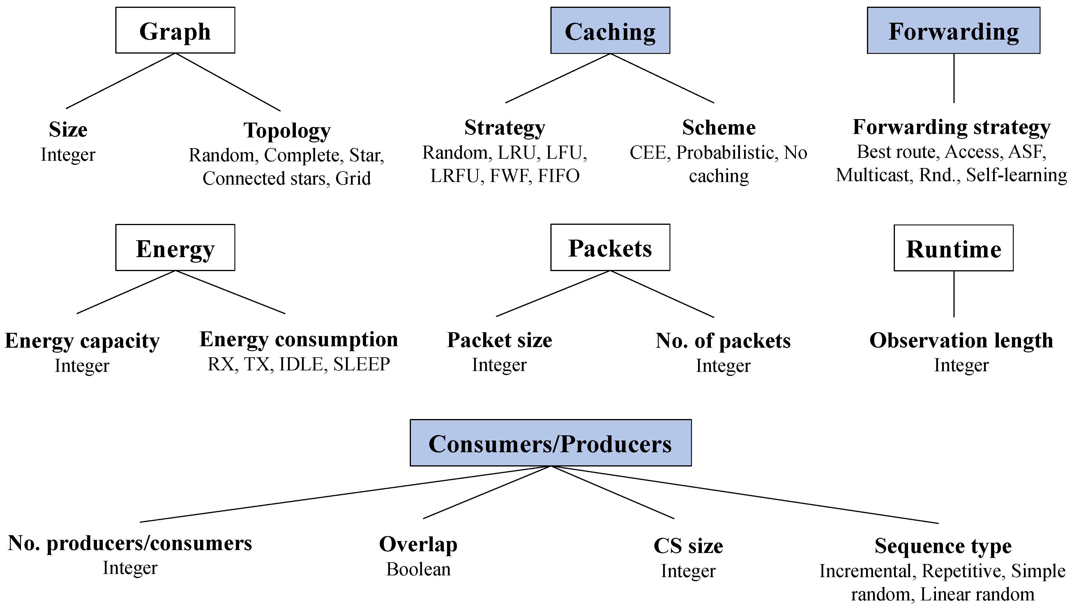
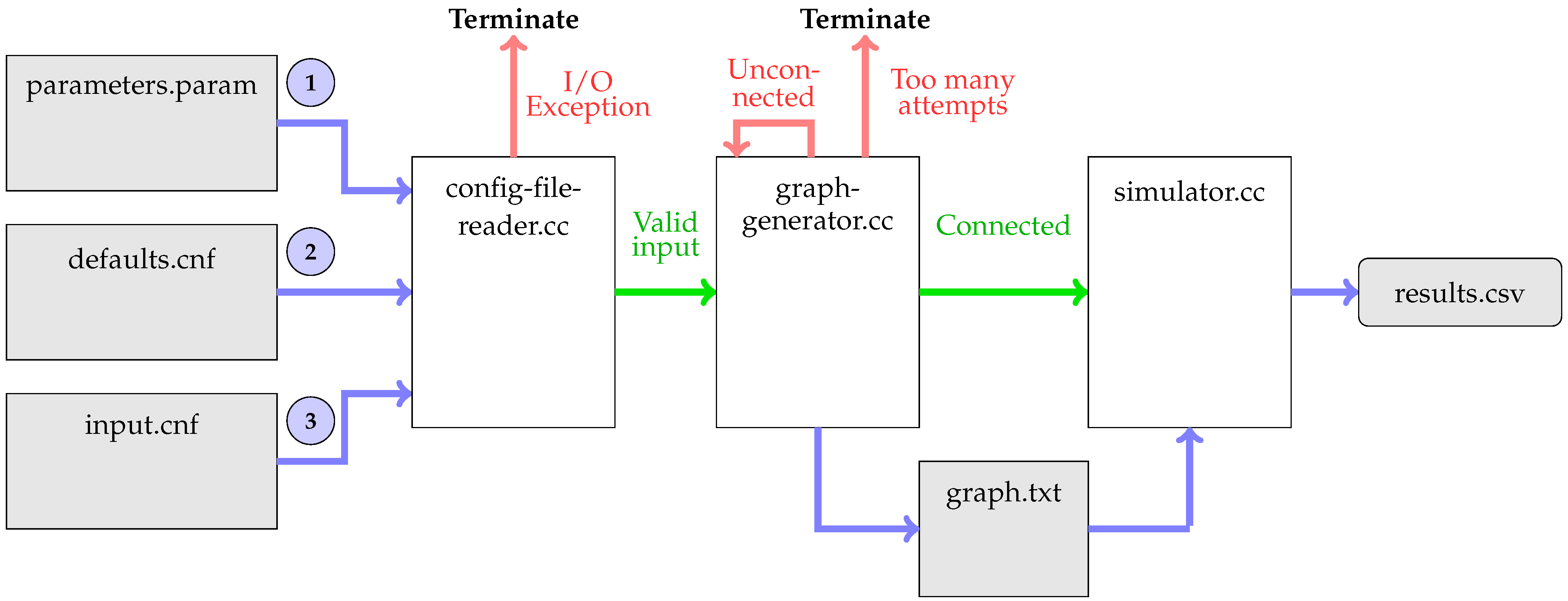
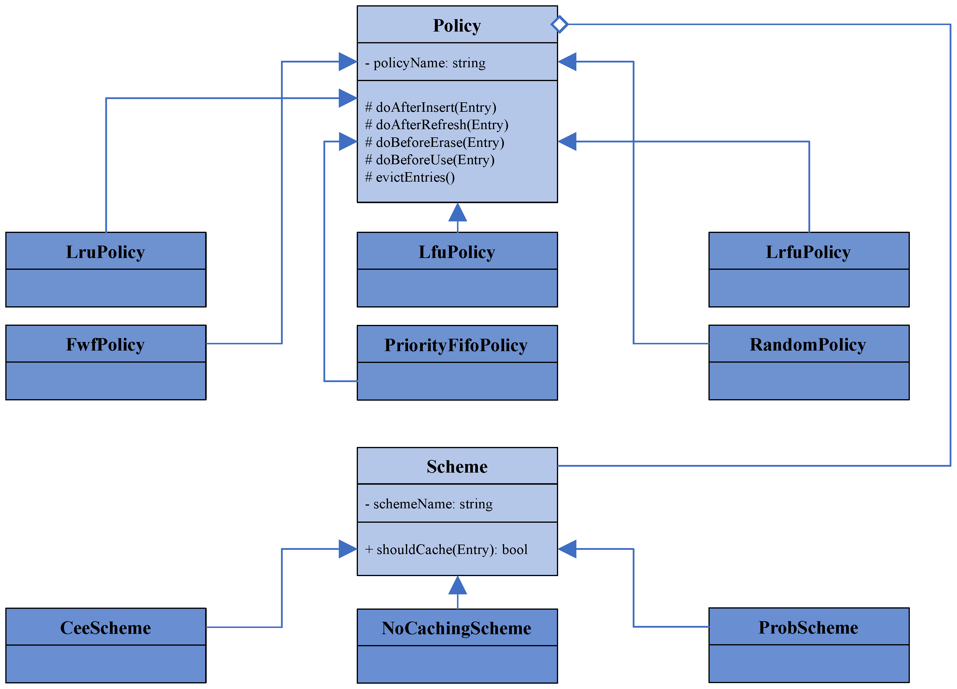
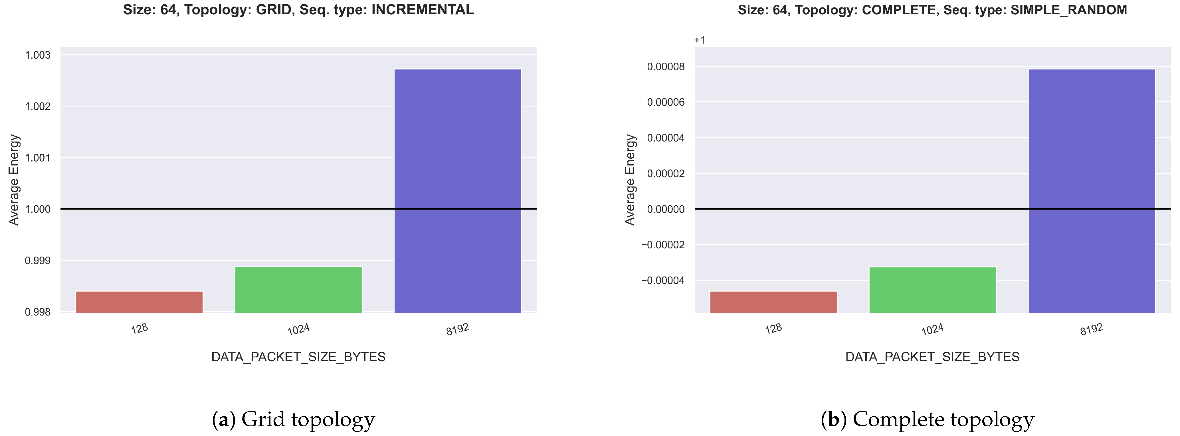
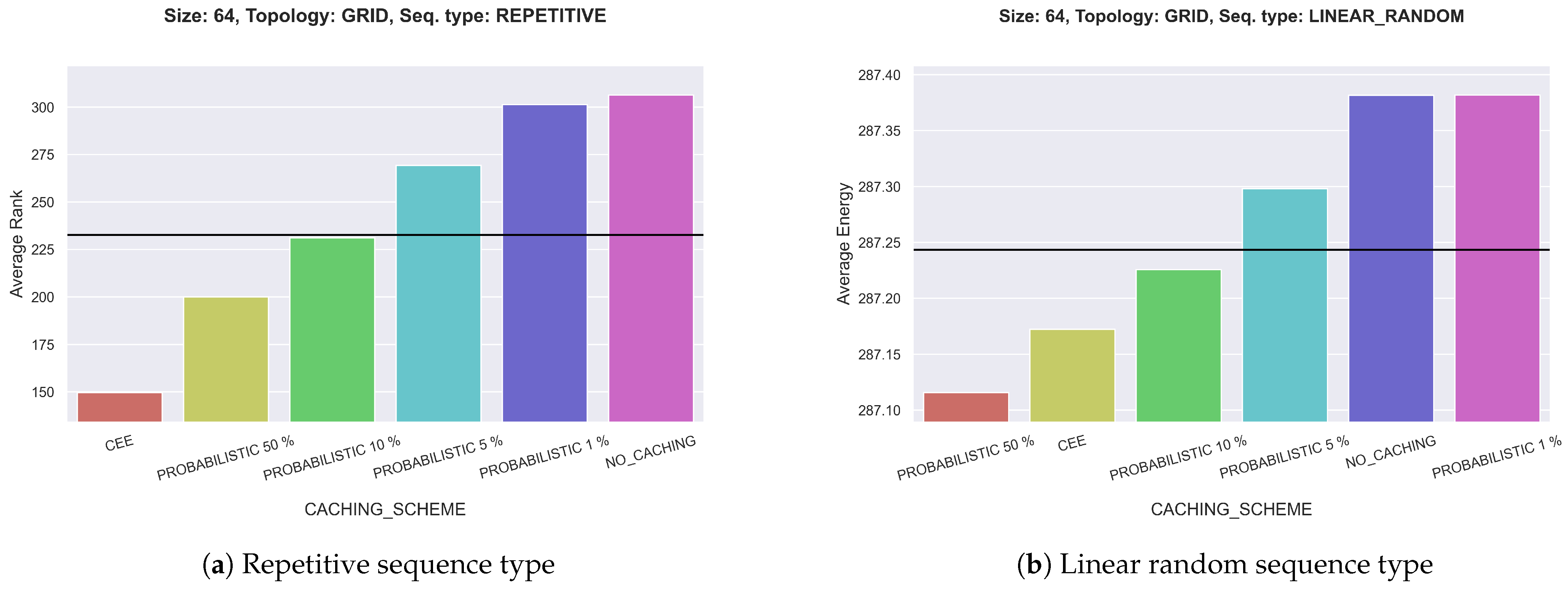
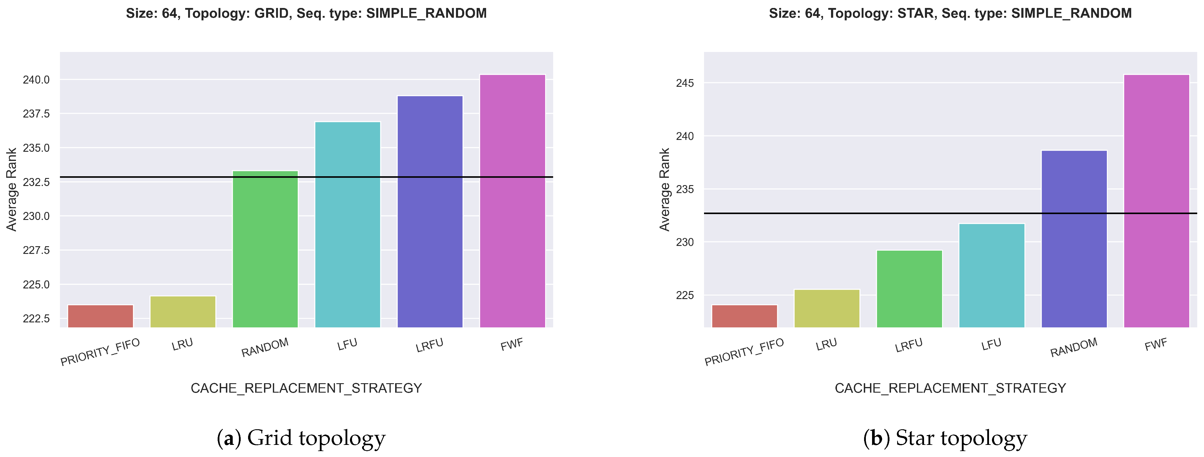
Table 1.
An example of a results.csv file for batch-1/graph-size=16/run0/run0.
| Category | Amount | Unit |
|---|---|---|
| Energy per node | 235.515 | J |
| Total consumed energy | 3768.24 | J |
| Standard deviation | 81.3037 | J |
| Min energy | 81.9 | J |
| Max energy | 409.604 | J |
Table 2.
Part of an example table for ranks of the sorted list of variable parameters. The example is for connected stars, size 4 and REPETITIVE. Row 3 and 4 receive the same rank because the energy consumption is equal. Since rank 4 is skipped, the next assigned rank is 5.
Table 2.
Part of an example table for ranks of the sorted list of variable parameters. The example is for connected stars, size 4 and REPETITIVE. Row 3 and 4 receive the same rank because the energy consumption is equal. Since rank 4 is skipped, the next assigned rank is 5.
| Rank | Average Energy | Packet Size | Caching Strategy | … |
|---|---|---|---|---|
| 1 | 122.85575 | 128 | LRFU | |
| 2 | 122.8565 | 128 | FWF | |
| 3 | 122.85725 | 128 | LRU | |
| 3 | 122.85725 | 128 | RANDOM | … |
| 5 | 122.85757 | 128 | FWF | |
| … | … | … | … |
Disclaimer/Publisher’s Note: The statements, opinions and data contained in all publications are solely those of the individual author(s) and contributor(s) and not of MDPI and/or the editor(s). MDPI and/or the editor(s) disclaim responsibility for any injury to people or property resulting from any ideas, methods, instructions or products referred to in the content. |
© 2024 by the authors. Licensee MDPI, Basel, Switzerland. This article is an open access article distributed under the terms and conditions of the Creative Commons Attribution (CC BY) license (https://creativecommons.org/licenses/by/4.0/).
Share and Cite
MDPI and ACS Style
Papenfuß, D.; Gerlach, B.; Fischer, S.; Hail, M.A. Enhancing Energy Efficiency in IoT-NDN via Parameter Optimization. Future Internet 2024, 16, 61. https://doi.org/10.3390/fi16020061
AMA Style
Papenfuß D, Gerlach B, Fischer S, Hail MA. Enhancing Energy Efficiency in IoT-NDN via Parameter Optimization. Future Internet. 2024; 16(2):61. https://doi.org/10.3390/fi16020061
Chicago/Turabian StylePapenfuß, Dennis, Bennet Gerlach, Stefan Fischer, and Mohamed Ahmed Hail. 2024. "Enhancing Energy Efficiency in IoT-NDN via Parameter Optimization" Future Internet 16, no. 2: 61. https://doi.org/10.3390/fi16020061
Note that from the first issue of 2016, this journal uses article numbers instead of page numbers. See further details here.