
An Imbalanced Sequence Feature Extraction Approach for the Detection of LTE-R Cells with Degraded Communication Performance


1
School of Computer and Information Technology, Beijing Jiaotong University, Beijing 100044, China
2
National Engineering Research Center for Digital Construction and Evaluation Technology of Urban Rail Transit, China Railway Design Corporation, Co., Ltd., Tianjin 300308, China
*
Author to whom correspondence should be addressed.
Future Internet 2024, 16(1), 30; https://doi.org/10.3390/fi16010030
Submission received: 20 December 2023
/
Revised: 8 January 2024
/
Accepted: 9 January 2024
/
Published: 16 January 2024
Abstract
:Within the Shuo Huang Railway Company (Suning, China ) the long-term evolution for railways (LTE-R) network carries core wireless communication services for trains. The communication performance of LTE-R cells directly affects the operational safety of the trains. Therefore, this paper proposes a novel detection method for LTE-R cells with degraded communication performance. Considering that the number of LTE-R cells with degraded communication performance and that of normal cells are extremely imbalanced and that the communication performance indicator data for each cell are sequence data, we propose a feature extraction neural network structure for imbalanced sequences, based on shapelet transformation and a convolutional neural network (CNN). Then, to train the network, we set the optimization objective based on the Fisher criterion. Finally, using a two-stage training method, we obtain a neural network model that can distinguish LTE-R cells with degraded communication performance from normal cells at the feature level. Experiments on a real-world dataset show that the proposed method can realize the accurate detection of LTE-R cells with degraded communication performance and has high practical application value.
1. Introduction
In recent years, due to the rapid development of the Chinese economy, demand for the transportation of goods has also rapidly increased, bringing great challenges to China’s transportation industry. In this situation, heavy haul railways have become a main development direction for freight railways [1]. Heavy haul trains have bigger load-carrying capacities and longer lengths, making them more difficult to operate. The existing wireless communication system, based on the global system of mobile communications for railways (GSM-R), has the disadvantages of insufficient bandwidth, poor anti-interference ability, and insufficient security [2]. Given this, Shuo Huang Railway applies the long-term evolution for railways (LTE-R) network to carry core wireless communication services, such as the synchronous control and wireless reconnection of heavy haul trains.
The LTE-R wireless communication system carries core communication services for heavy haul trains. Therefore, the communication performance of LTE-R cells directly affects the operational safety of heavy haul trains. At present, Shuo Huang Railway mainly collects communication performance indicator data for each cell using drive tests and then manually screens for cells with degraded communication performance by observing the deterioration of key performance indicators. However, due to the large amount of drive test data, this traditional manual analysis detection method is inefficient and accuracy largely depends on the personal abilities and work status of the operational and maintenance personnel [3]. In fact, it is difficult to accurately determine whether a certain cell has experienced communication performance degradation solely based on road test data. The evolved radio access bearer (E-RAB) abnormal release rate (EARR) of LTE-R core communication services is a more practical indicator for evaluating the communication performance of LTE-R cells [2]. But EARR is a statistical indicator that is difficult to obtain in real time. Therefore, it is necessary to develop more efficient and intelligent methods for the detection of LTE-R cells with degraded communication performance by establishing the accurate mapping relationship between the drive test data and EARR.
Some experts and scholars have already studied detection methods for abnormal wireless communication performance. These detection methods are mainly divided into two types: shallow model methods [4,5,6,7] and deep model methods [8,9,10,11,12]. Shallow model methods utilize traditional shallow model machine learning methods to detect abnormal wireless communication performance. However, shallow model methods have shortcomings in extracting complex nonlinear patterns from data. With the continuous development of deep learning technology, more researchers are attempting to use deep model methods to detect abnormal wireless communication performance. Since the mapping relationship between drive test data and EARR is a complex nonlinear mapping relationship, and deep model methods have advantages in dealing with the problem of complex nonlinear mapping [13], this paper chooses to use deep model methods to establish this mapping relationship. Furthermore, due to the high reliability of the LTE-R communication system, records for cells with degraded communication performance are very rare (the ratio of normal data to abnormal data is close to 30:1), so the main difficulty in detecting LTE-R cells with degraded communication performance is how to build an imbalanced data classification model with high classification accuracy.
In order to solve the problem of detecting LTE-R cells with degraded communication performance, we fully consider the characteristic of communication performance indicator data being sequentially distributed along railways, and we treat the detection problem as an imbalanced sequence data classification problem. Then, based on the basic principle of shapelet transformation, we realize the feature extraction of sequence data by transforming CNN. In addition, to solve the problem of imbalanced data classification, we set the loss function based on the Fisher criterion and propose a two-stage training method based on contrastive loss and the differential evolution algorithm. Experiments on a real-world dataset showed that the proposed method can accurately detect LTE-R cells with degraded communication performance, which could provide an effective technological means for improving the efficiency of LTE-R network operation and maintenance and ensuring the safety of railway operations.
The main contributions of this paper can be highlighted as follows.
- Based on the principle of shapelet transformation, this paper designed a neural network structure that can extract morphological features of sequence data by transforming CNN neural networks.
- In the detection of LTE-R cells with degraded communication performance, considering the class imbalanced problem, a two-stage training method is proposed to make the features extracted by the trained feature extraction network meet Fisher criterion as much as possible.
- By using machine learning methods, the mapping relationship between the drive test data and the abnormal release rate of LTE-R core communication services was established, which provides a powerful tool for the operation and maintenance of LTE-R network.
2. Related Work
2.1. Abnormal Wireless Communication Performance Detection
Accurate detection of abnormal wireless communication performance is the foundation of wireless network operation and maintenance. Presently, many detection methods have been proposed to solve this problem, which can be divided into two types: shallow model methods [4,5,6,7] and deep model methods [8,9,10,11,12]. For example, Chernogorov et al. [4] analyzed the event sequences reported by mobile terminals to base stations and utilized the N-gram analysis method to reduce dimensionality and classify the data, ultimately achieving the detection of abnormal wireless communication performance. Chernov et al. [5] also analyzed the event sequences reported by mobile terminals to base stations and compared the accuracy of multiple anomaly detection methods for detecting abnormal wireless communication performance caused by random access channel anomalies. Miao et al. [6] achieved high detection accuracy by using the kernel density-based local outlier factor (LOF) algorithm to detect cells with degraded communication performance. Safaei et al. [7] designed a decentralized abnormal wireless communication performance detection method based on the local outlier factor algorithm to perform abnormal detection in wireless sensor networks (WSNs). The above studies all used traditional shallow model machine learning methods to detect abnormal wireless communication performance. However, the development of neural networks, especially deep learning technologies, has provided a new research direction for the detection of abnormal wireless communication performance. Premkumar et al. [8] proposed a deep learning-based lightweight distributed denial of service attack detection scheme to detect the anomaly in the data forwarding phase of WSN. Regin et al. [9] compared the performance of the convex hull algorithm, naive Bayes algorithm, and CNN in the detection of abnormal nodes in WSN, and proved that CNN has the best detection performance. Kuadey et al. [10] proposed a framework based on a long short-term memory (LSTM) deep learning technique that detects DDoS attacks in a 5G network. Huan et al. [14] proposed an unsupervised spectrum anomaly detection method based on the variational autoencoder (VAE) and aimed to detect anomalies in unauthorized frequency bands in a wireless communication network. Dahiya et al. [12] proposed a unique DDoS attack detection model, which combined the LSTM with the recurrent neural network (RNN) to construct the detection model, and utilized the opposition learning-based seagull optimization algorithm (OLSOA) to optimize the weight of the RNN for more accurate detection of DDoS attacks. Qu et al. [3] proposed a dual encoder denoising autoencoder (DEDAE) neural network based on the non-dominated sorting genetic algorithm-III (NSGA-III) and generative adversarial network (GAN), which can detect LTE-R cells with degraded wireless communication performance.
Since wireless communication network performance degradation is the result of many factors [2], the detection of abnormal wireless communication performance is usually a complex nonlinear problem. This paper chooses the deep model method to perform the detection of LTE-R cells with degraded communication performance.
2.2. Imbalanced Data Classification
Real-world datasets are mostly imbalanced and the lack of minority class samples can cause bias in classification models that have been constructed using classification methods [15]. Currently, imbalanced data classification methods can be divided into two groups: data-level and algorithm-level methods. There are many methods for solving imbalanced data classification problems at the data level, which can also mainly be divided into two types: undersampling [16,17,18] and oversampling [19,20,21]. However, although data-level methods can effectively deal with the imbalanced data problem, when data are extremely imbalanced, the excessive generation or reduction of data can alter the distribution of the original data while the limited generation or reduction of data cannot change the problem of data imbalance. Due to the high reliability of the LTE-R wireless communication system, datasets for the detection of LTE-R cells with degraded communication performance are extremely imbalanced. Therefore, algorithm-level methods should be considered for realizing the detection of cells with degraded performance. The main idea of algorithm-level methods is to directly modify the learning process of classification methods to improve sensitivity to minority classes. Recently, shallow-model algorithm-level methods have achieved great success in the fields of imbalanced data classification and fault detection [22,23,24]. However, they have significant limitations in processing high-dimensional data and expressing complex nonlinear patterns. The emergence of neural networks and deep learning technologies has provided new and effective ways to solve imbalanced data classification problems, and many new solutions for imbalanced data classification have emerged. Zhang et al. [25] applied the cost-sensitive loss function to a deep belief network (DBN) and utilized the evolutionary algorithm to find the optimal misclassification cost, thus realizing the classification of imbalanced data. Geng et al. [26] proposed a cost-sensitive deep convolutional neural network (CNN) and experimentally demonstrated the superiority of this method in imbalanced time series classification. The above cost-sensitive method involves strengthening the recognition ability of the model to minority class samples by introducing the cost-sensitive factor in the training process. However, cost-sensitive factors are often difficult to determine, and these kinds of empirical risk minimization methods often have limited effectiveness when data are extremely imbalanced. Therefore, when the data are extremely imbalanced, some researchers utilize autoencoder (AE) neural networks or generative adversarial networks (GANs) to build data models for majority class samples. They then determine whether the data are abnormal based on the reconstruction error. Jinwon et al. [27] discussed how to use AE and the variational autoencoder (VAE) neural network to detect abnormal data. Thomas et al. [28] utilized GAN to guide the training process of AE, which can help AE learn the data distribution of majority class data. Cheng et al. [29] proposed an improved autoencoder for unsupervised anomaly detection, which optimizes the anomaly detection task by integrating anomaly detection-based loss and autoencoder reconstruction loss. Furthermore, this method can learn representations that preserve local data structures to avoid feature distortion. But, these unsupervised anomaly detection methods will overlook the information contained in minority class samples. Given the above, constructing specific optimization objective functions to increase the distance between samples of different categories becomes an effective solution. Wang et al. [30] designed a change detection algorithm based on Siamese networks for optical aerial images, and utilized an improved contrastive loss–focal contrastive loss (CFCL) to train the model, which can solve the data imbalanced problem. Jiao et al. [31] proposed an autonomous anomaly detection technique for multivariate time series data based on a novel self-supervised contrastive loss, which outperforms state-of-the-art anomaly detection approaches and exhibits robustness when training data are contaminated.
The above deep learning-based imbalanced data classification methods have achieved great success in different fields. But, to realize the accurate detection of LTE-R cells with degraded communication performance, it is still necessary to study the corresponding neural network structure and training method based on the characteristics of imbalanced sequence data.
3. Preliminaries
3.1. Data Description
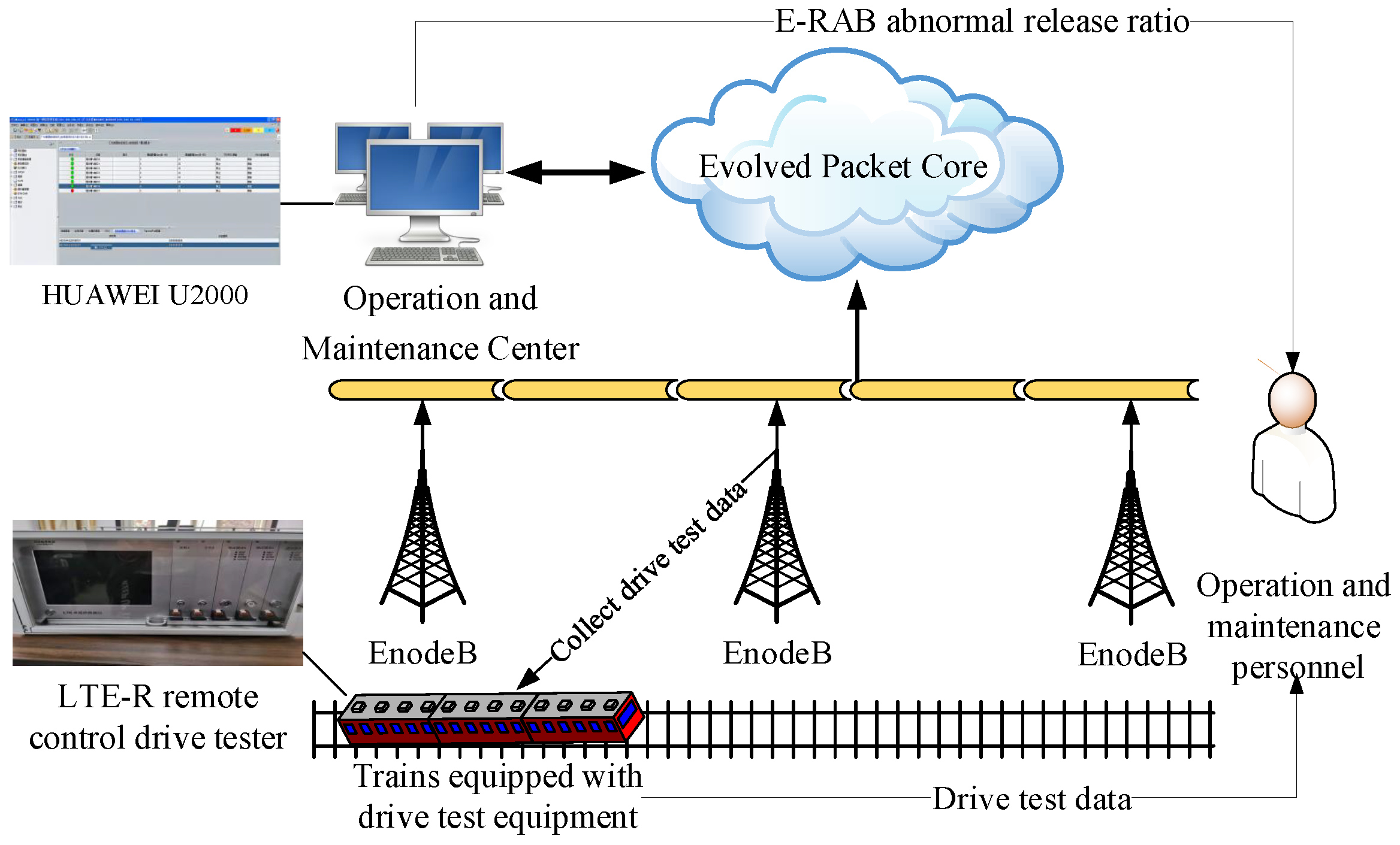
In this study, we chose relevant data for the operation and maintenance of the Shuo Huang Railway LTE-R network to construct a dataset for detecting cells with degraded communication performance. There are two main sources of Shuo Huang Railway operation and maintenance data: drive test data and abnormal release data from the E-RAB for each wireless communication service exported from the LTE-R Operation and Maintenance Center (OMC). Drive tests are the most commonly used methods for measuring the wireless network communication status along the Shuo Huang Railway. They are usually carried out by operation and maintenance personnel, who use measurement equipment to collect wireless communication performance indicator data from the user equipment (UE) side along the Shuo Huang Railway. At present, the OMC used in the Shuo Huang Railway LTE-R system is the Huawei u2000 (Huawei, Shenzhen, China),which can record historical key performance indicator data from the LTE-R system, thereby achieving unified management and maintenance of the network element layer and the network layer of the LTE-R network [32]. Figure 1 shows the source of Shuo Huang Railway operation and maintenance data.
Drive test data contain a lot of information, including the reference signal receiving power (RSRP), reference signal receiving quality (RSRQ), signal-to-interference-plus-noise ratio (SINR), geographic location information, physical-layer cell identity (PCI), etc. Among these metrics, RSRP and SINR measure the communication status of LTE-R cells from the perspectives of signal strength and noise, respectively, while RSRQ is an important indicator for cell handover and reselection. Therefore, we selected RSRP, RSRQ, and SINR as the metrics for judging whether communication performance deterioration occurs in LTE-R cells. Furthermore, PCI was selected to categorize drive test data according to the LTE-R cells they belong to.
Using data exported from the OMC system, many statistical values related to LTE-R communication performance can be obtained, such as throughput, latency, dropout rate, etc. In this paper, we focused on the E-RAB abnormal release rate. The successful establishment of an E-RAB shows that eNodeB has allocated wireless resources and radio bearers to the UE. Therefore, the E-RAB abnormal release rate represents the ability of eNodeB or a cell to carry services and can be used to evaluate the operational status of eNodeB or cells [2]. In the Shuo Huang Railway LTE-R system, the E-RAB abnormal release rate is calculated separately, according to the different wireless communication service types. The different types of wireless communication services on the Shuo Huang Railway are assigned a quality-of-service (QoS) class identifier (QCI) value, ranging from 1 to 7. The different QCI values and their corresponding communication services for the Shuo Huang Railway LTE-R system are shown in Table 1.
From Table 1, it can be seen that communication services with a QCI of 1 have the highest QoS priority. The higher the QoS priority, the more important the communication service and the more resources it can obtain from wireless communication resource allocation. Therefore, we chose to use the E-RAB abnormal release rate (EARR) of communication services with a QCI of 1 as the only indicator to evaluate whether cells had experienced communication performance degradation. If the E-RAB abnormal release rate was greater than a certain threshold, the corresponding cell was considered to have degraded communication performance.
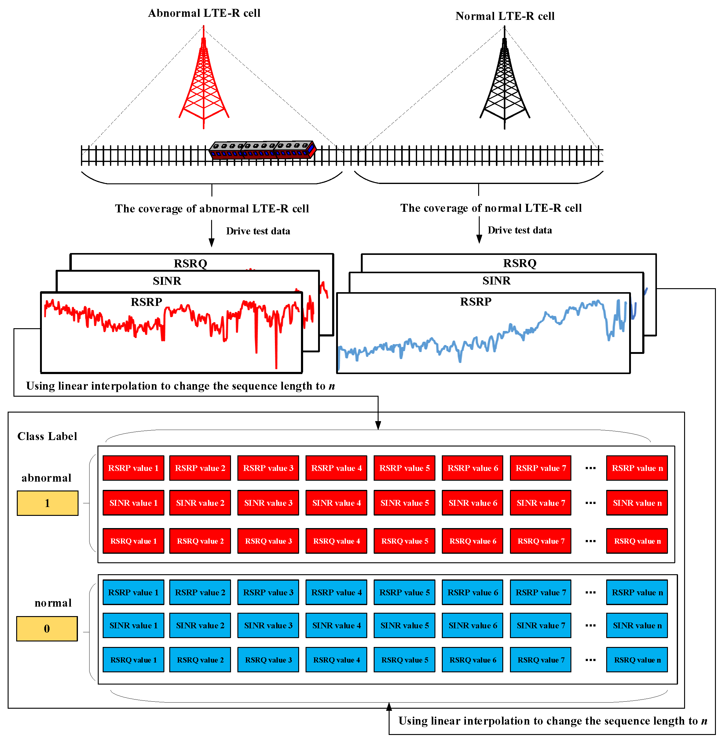
In this paper, the drive test data of each LTE-R cell are taken as feature values and the linear interpolation method is used to interpolate the drive test data into sequences of the same length. Then, based on the EARR of the communication services with a QCI of 1 exported by the OMC, the drive test data are labeled as abnormal or normal, and a dataset is constructed for the detection of LTE-R cells with degraded communication performance. Figure 2 shows the construction process for this dataset.
As can be seen from Figure 2, the drive test data for the selected performance indicators are sequence data distributed along the railway. In addition, due to the high reliability of the LTE-R network, the constructed dataset for the detection of LTE-R cells with degraded communication performance is a typical imbalanced sequence classification dataset.
3.2. Shapelet and Shapelet Transformation
As defined in [33], shapelets are subsequences of sequence datasets that can maximally distinguish between sequence classes, assuming M is the length of the shapelet and N is the length of the sequence in the sequence dataset. Broadly speaking, shapelets are not necessarily subsequences of sequence data in the strictest sense. Any sequence that can distinguish between sequence classes in terms of shape and has a length that satisfies can be considered as a shapelet of a sequence dataset.
For the convenience of these calculations, the distance between the i-th sequence data in a one-dimensional sequence dataset, , and the k-th shapelet, , is defined by Formula (1).
In (1), represents the distance between and . Accordingly, the smallest distance between all J subsequences of length M in and is .
After finding the K optimal shapelets in the one-dimensional sequence dataset, the distance between the K optimal shapelets and certain sequence data can be obtained using (1). These distances are used as new features of the sequence data, which map the sequence data to a new feature space. The above process is also called shapelet transformation. Through shapelet transformation, we can transform the one-dimensional sequence dataset X into D, where D is , is and the value of y is 0 or 1. In general, the value of K is much smaller than N, so shapelet transformation can effectively reduce the dimensions of sequence data.
The approach proposed in this paper extracts corresponding shapelets from the drive test data of each LTE-R cell in a supervised manner by modifying the CNN network and performing shapelet transformation to realize feature extraction.
4. Methodology
4.1. The Overall Framework of Our Approach
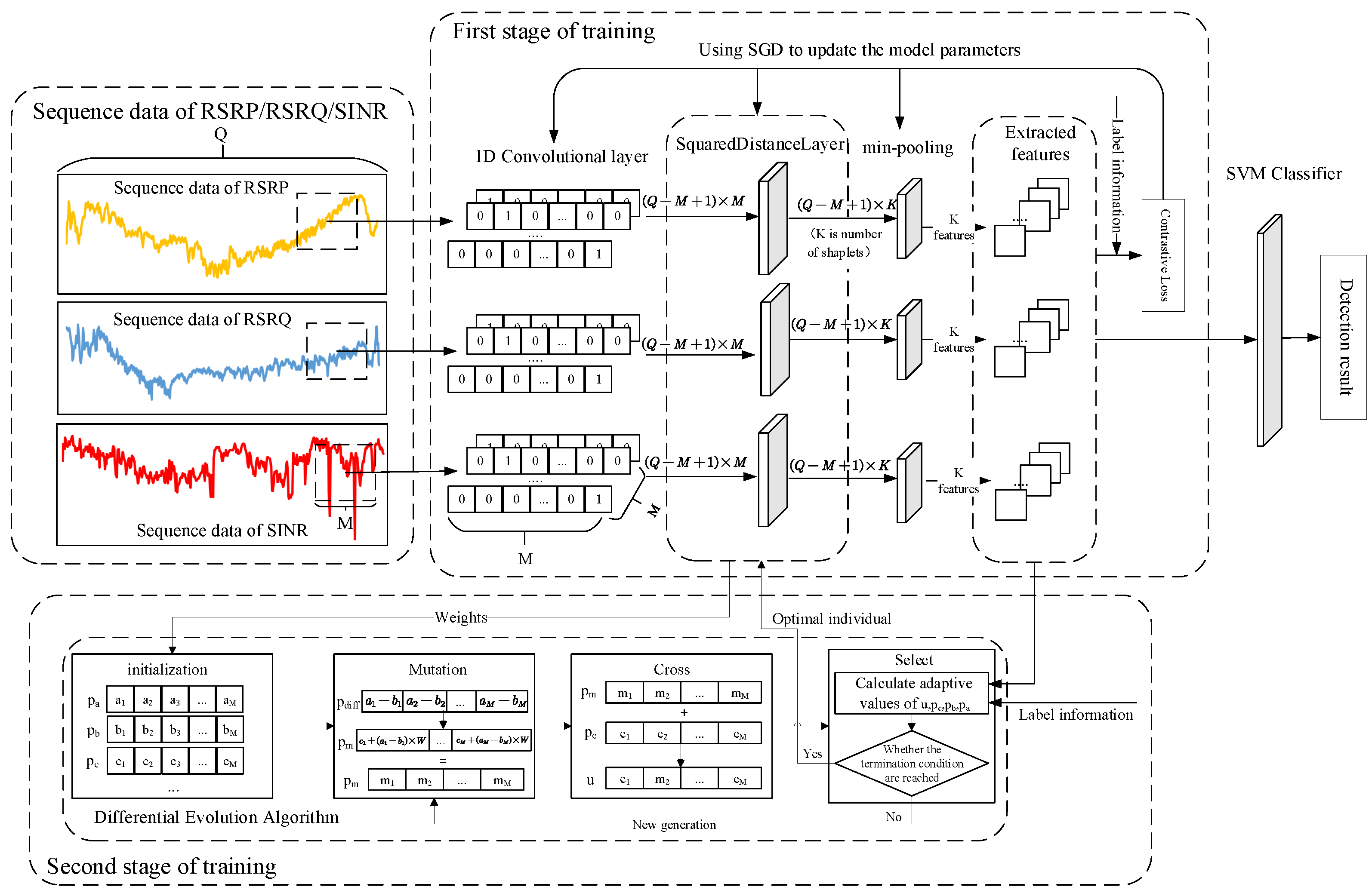
The idea of shapelet transformation is to separate the shapelet extraction process from the classification method. Following dimensionality reduction through shapelet transformation, sequence data can be classified using a general classifier. This also establishes the overall framework of the sequence data classification method, based on shapelet transformation. The proposed feature extraction method for imbalanced sequences follows this framework but also includes the processing of imbalanced sequence data. Therefore, the detection method for LTE-R cells with degraded communication performance proposed in this paper is divided into two steps: (1) Using the modified CNN to extract features from key performance indicator data within the drive test data; (2) Using a general classifier (in this case, SVM) to classify data after feature extraction and achieve the detection of degraded cells. The overall framework of the proposed approach is shown in Figure 3.
From Figure 3, it can be seen that for the one-dimensional sequence dataset composed of the measured values of each key performance indicator from the drive test data, the input one-dimensional sequence data are first passed through a one-dimensional convolutional layer to obtain every subsequence of the input sequence data. Afterward, these subsequences are input into a squared distance layer, in which the weights of the neural network layer represent the shapelets of the input sequence data. Therefore, the role of this layer is equivalent to calculating the distance between each shapelet and each subsequence of the input sequence. After passing through the distance calculation layer, the distance between each shapelet and each subsequence passes through a min pooling layer and the output is the distance between each shapelet and the input sequence data, which is the result of shapelet transformation. As mentioned in Section 3.1, we selected three key performance indicators from the drive test data to use as input data: RSRP, RSRQ, and SINR. In order to perform the shapelet transformation of these three indicator sequences simultaneously, the shapelet transformation results of each indicator sequence are merged in the output layer to form a unified model. In order to obtain shapelets that can maximally distinguish different class sequences, we propose a two-stage training method to train the model. In the first stage, the contrastive loss [34] is used as the loss function to train the feature extraction network. In the second stage, the differential evolution algorithm is introduced to optimize the weights of the squared distance layer while setting an optimization objective based on the Fisher criterion. The entire model training process can also be regarded as the process of finding the optimal shapelets for each sequence. At this point, feature extraction for the imbalanced multidimensional sequence dataset is complete. Finally, following feature extraction, the dataset is input into an SVM for classification, thereby achieving the detection of LTE-R cells with degraded communication performance.
4.2. A Feature Extraction Network-Based CNN
CNNs are important variants of neural networks, which have been widely used in many fields, such as computer vision, natural language processing, and image and sequence feature extraction [35]. CNNs mainly include convolutional layers, pooling layers, activation layers, and other structures. As shown in Figure 3, in this paper, we utilized a one-dimensional convolutional layer and a pooling layer to construct a feature extraction network. The main principles of one-dimensional convolutional layers and pooling layers are as follows.
- One-dimensional convolutional layer.Convolutional layers perform discrete convolution operations on input data through convolutional kernels, thereby extracting the features of the input data. Multiple convolution kernels can be used to extract different features of input data. Assuming that is a one-dimensional convolutional kernel, is a data record and is the result of one-dimensional convolutional. The j-th element of y is as shown in Formula (2).where N denotes the dimensions of the data record and M denotes the size of the convolutional kernel.
- Pooling layersIn CNNs, pooling layers are used to reduce the size of feature maps while expanding the receptive fields of the next-level neural networks. There are several types of pooling layers, including mean pooling, max pooling, stochastic pooling, and min pooling.
The feature extraction network proposed in this article was constructed based on the CNN network structure. In this feature extraction network, the convolutional calculation process of the one-dimensional convolutional network is used to extract all of the specific lengths of the subsequences from the input data. Afterward, we designed a neural network layer that can calculate the distance between each shapelet and subsequence of input data, equal in length to each shapelet. Finally, a min pooling layer is used to obtain the distance between each shapelet and the input data (please refer to Formula (1)).
Assuming that the input sequence length is 500, the number of shapelets is 7, and the shapelet length is 400, the proposed feature extraction network is as shown in Table 2.
The main steps of the feature extraction network proposed in this paper are as follows.
Step 1: Extract the subsequences of the input data. By designing a convolutional kernel for a one-dimensional convolutional neural network, we can extract all subsequences that are the same lengths as the shapelets from the input data. Assuming that the length of the shapelet to be extracted is M, the length and number of convolution kernels should also both be M. At this point, the i-th element of the j-th convolution kernel is as shown in Formula (3).
After determining the weights of all convolutional kernels, they are locked, meaning that they do not participate in the subsequent training process. Using the above processing, all subsequences of input data that are of the same length as the shapelets can be obtained. For example, when the length of a shapelet is M and the length of the input data sequence is Q, we can obtain subsequences with a length of M.
Step 2: Calculate the distance between each shapelet and each subsequence. In order to calculate the distance between each shapelet and the subsequences obtained in Step 1, we designed a squared distance neural network layer to achieve squared distance calculation. The number of weights in this layer depends on the length and number of shapelets. For example, if the length of a shapelet is M and the number of shapelets is K, then the number of weights in the squared distance layer is . In fact, these weights can be regarded as the shapelets corresponding to the input data. Therefore, the output of the squared distance layer is the squared distance between each shapelet and each subsequence of input data.
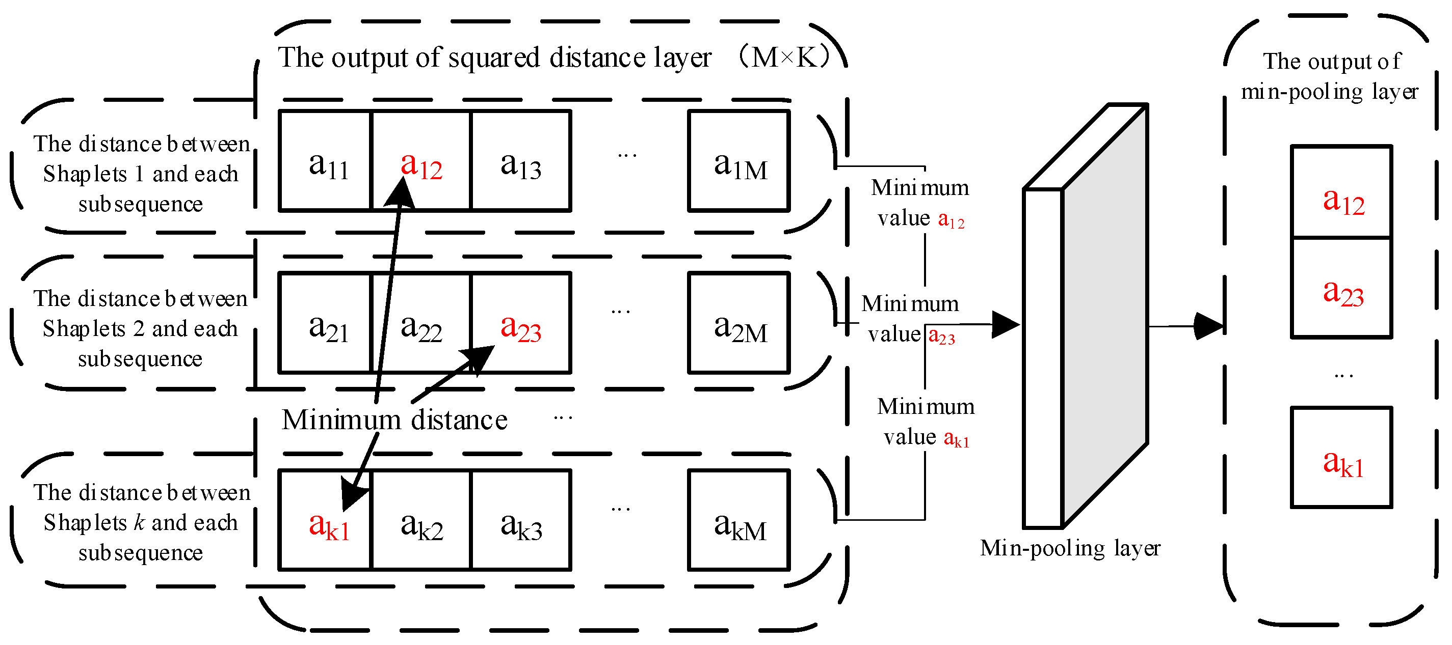
Step 3: Calculate the minimum distance between each shapelet and each subsequence. According to Section 3.2, to obtain the distance between each shapelet and the input data, it is necessary to calculate the minimum distance between each shapelet and each subsequence. The above goals can easily be achieved via the min pooling layer. Figure 4 illustrates the working principles of min pooling.
As can be seen in Figure 4, after passing through the min pooling layer, the output of the squared distance layer can obtain a vector composed of the distance between each shapelet and the input data, i.e., the extracted features.
Through the above steps, the feature extraction network proposed in this paper can complete the shapelet transformation of input data, thereby extracting features.
4.3. Optimization Objective for the Feature Extraction of Imbalanced Sequences
Due to the fact that the number of LTE-R cells with degraded communication performance is much smaller than the number of normal cells, the detection of LTE-R cells with degraded communication performance is a typical imbalanced sequence classification problem.
Traditional neural networks for classification often aim to minimize empirical risk during training, such as the cross-entropy loss function. However, when training imbalanced data, the classification information that minority class samples can provide is limited due to the insufficient number of minority class samples. If empirical risk minimization is chosen as the optimization objective of model training, it causes model bias. Therefore, when conducting model training in this paper, we considered optimization objectives based on the Fisher criterion to solve the imbalanced data problem.
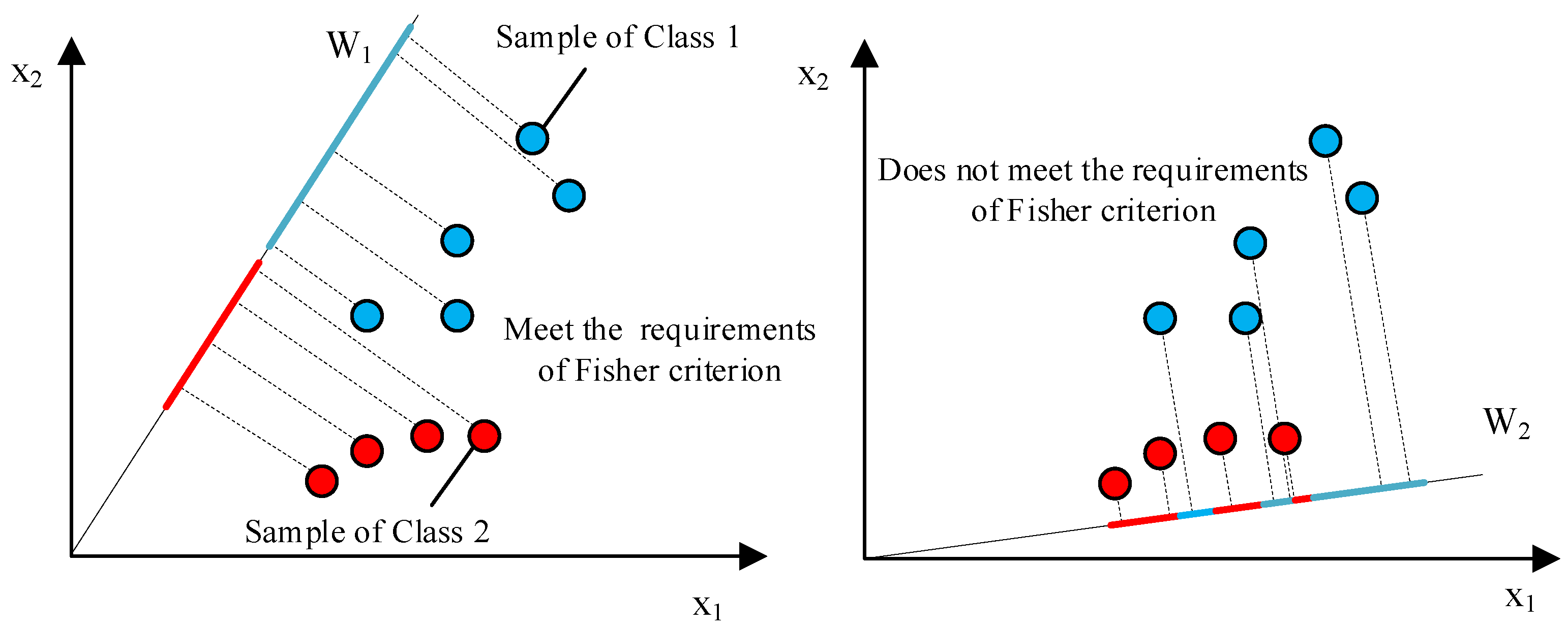
The Fisher criterion was proposed by R. A. Fisher in 1936 [36]. The basic idea of the Fisher criterion is to find a certain projection subspace in a feature space so that all feature points can have the best classification performance in that subspace. The basic principle of the Fisher criterion is shown in Figure 5.
Figure 5 shows the projection of a two-dimensional dataset onto a one-dimensional vector. By comparing different projection vectors ( and ), it can be seen that the classification performance of the data samples after projection onto is better than that after projection onto . It can also be seen that the basic idea of the Fisher criterion is that the results of a projection function should satisfy the following conditions: the between-class scatter after projection should be as large as possible and the within-class scatter should be as small as possible. In fact, the feature extraction network proposed in this paper can be regarded as a projection function, so the optimization objectives for training the network include the following two aspects:
- Within-class scatter.Considering that the problem studied in this paper is a binary classification problem and assuming that the two classes are and , then is the number of samples in class . So, the within-class scatter matrix of class is as shown in Formula (4).In (4), is the mean vector of . The overall within-class scatter matrix is as shown in Formula (5).The trace of is the overall within-class scatter of and . Assuming that is a matrix, is the element of at row i and column j and represents the trace of . The trace of is as shown in Formula (6).
- Between-class scatter.The between-class scatter matrix between and is as shown in Formula (7).The trace of is the between-class scatter between and .
After obtaining the within-class scatter and between-class scatter, these two values can be combined by division to form the loss function for training feature extraction networks in order to reach the objectives of minimizing within-class scatter and maximizing between-class scatter. The loss function for training the proposed feature extraction network is as shown in Formula (8).
During the model training process, the smaller the value of the loss function, the better the corresponding model performance. By observing the calculation process of this loss function, it can be seen that its calculation results are not affected by the number of samples in each category. Therefore, this loss function can be applied to the classification of imbalanced data.
4.4. Model Training
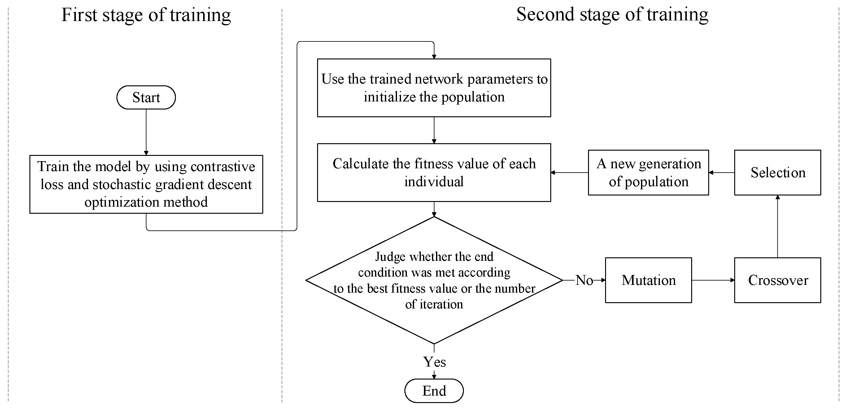
To make the features extracted by the proposed feature extraction network meet the optimization objectives defined in Section 4.3 as much as possible, we propose a two-stage training method. Figure 6 demonstrates the flow of the two-stage training method.
In the first stage, we utilize the stochastic gradient descent (SGD) optimization method to optimize the model parameters and the loss function is contrastive loss. The SGD optimization method is used to train the feature extraction network proposed in Section 4.2. The contrastive loss is as shown in Formula (9).
where W is the weight of the model, N is the size of the training data, and represent the features of samples and , respectively, the value of Y is determined by the categories of samples and (if and do not belong to the same category, then , otherwise, ), is an abbreviation for (representing the Euclidean distance between and ), and M is the set threshold.
As can be seen in (9), when , the model training process can minimize the distance between and by adjusting parameters. When and the distance between and is greater than m, there is no need to optimize parameters. When the distance between and is less than m, the distance between and needs to be increased to m. Therefore, the use of contrastive loss can increase the scatter between different categories.
However, the contrastive loss function is mainly used to increase between-class scatter, without considering within-class scatter. According to the description in Section 4.2, shapelet transformation is mainly completed at the distance calculation layer. Therefore, in the second stage of training, we use the differential evolution (DE) algorithm and the training data to optimize the weights of the distance calculation layer in the first stage of training, with the goals of better meeting the requirements of the Fisher criterion and further improving the classification performance of the model.
The DE algorithm is an optimization algorithm based on swarm intelligence theory, which has the advantages of fast convergence speeds, high reliability, high efficiency, robustness, and strong global search ability [37]. It has been widely used in many optimization problems [38,39,40]. The main steps of the second stage of training are as follows.
Step 1: Population initialization. To achieve better optimization results, individuals in the initialized population should cover the solution space as much as possible. The range of the solution space is determined by the upper and lower of weights, while the dimensions of the individual vectors are related to the length and number of shapelets, assuming that the length and number of shapelets are M and K, respectively. We chose to focus on three key performance indicators from the drive test data, so the dimension of the individual vector is and the i-th individual in the initial population is , where is the number of individuals in the initial population. The j-th element in the individual vector is as shown in Formula (10).
Step 2: Fitness evaluation. In this paper, in order to calculate the fitness of an individual, firstly, the individual vector needs to be substituted into the distance calculation layer of the feature extraction network as the weights of the distance calculation layer. Then, the training data can be input into the feature extraction network for feature extraction. Finally, the extracted features and corresponding category information are substituted into Formula (8) to obtain the fitness of the individual vector.
Step 3: Mutation. In each round of evolution, a mutation operation is performed on all individuals in the current generation. If the mutated individual vector is , the mutation operation is as shown in Formula (11).
In (11), , , and are three different random individual vectors in the current generation g, where , and F is a constant between 0 and 1 that represents the scaling factor.
Step 4: Crossover. Some components of each individual vector are swapped with the corresponding mutation vector to obtain the crossover vector . For the j-th element of , the crossover operation is as shown in Formula (12).
In (12), represents the crossover probability (which is a real number between 0 and 1), D is the dimension of the individual vector, and is a random integer between 0 and 1.
Step 5: Selection. All individual vectors and their corresponding cross variables are substituted into the fitness function to obtain the individual vectors in the next generation. The selection operation is as shown in Formula (13).
Steps 2 to 5 are repeated until the number of iterations reaches the preset maximum value, and then the optimal individual is used as the weight of the distance calculation layer.
Using the above two-stage training method, we obtained a neural network that can extract features from the detection dataset of LTE-R cells with degraded communication performance. Then, simply using traditional classification methods, such as SVM, to classify the data after feature extraction can achieve high detection accuracy.
5. Experiments and Discussion
5.1. Experimental Data
As mentioned in Section 3.1, the experimental data in this paper are drive test data from the Shuo Huang Railway LTE-R network from September 2015 to August 2018, as well as the corresponding EARR data for communication services with a QCI value of 1 exported by the OMC system. Then, we preprocess these data as follows.
Firstly, we extract the data sequences of the key performance indicators (RSRP, RSRQ, and SINR) from the drive test data of each cell, based on the PCI value. Then, using the Lagrangian interpolation to interpolate these three data sequences into sequences with a length of 500, we regard the matrix as a record in the dataset. Finally, we label these records based on the EARR data for communication services with a QCI value of 1 for each cell. If the EARR value is greater than 2%, the cell is marked as an abnormal cell, otherwise, the cell is marked as a normal cell. Through the above process, we obtained the detection dataset of LTE-R cells with degraded communication performance, or the degradation detection dataset for short.
In our experiment, 70% of the data were selected as the training set, and the remaining 30% were used as the test set. Detailed information regarding the degradation detection dataset is shown in Table 3.
5.2. Experiment Settings
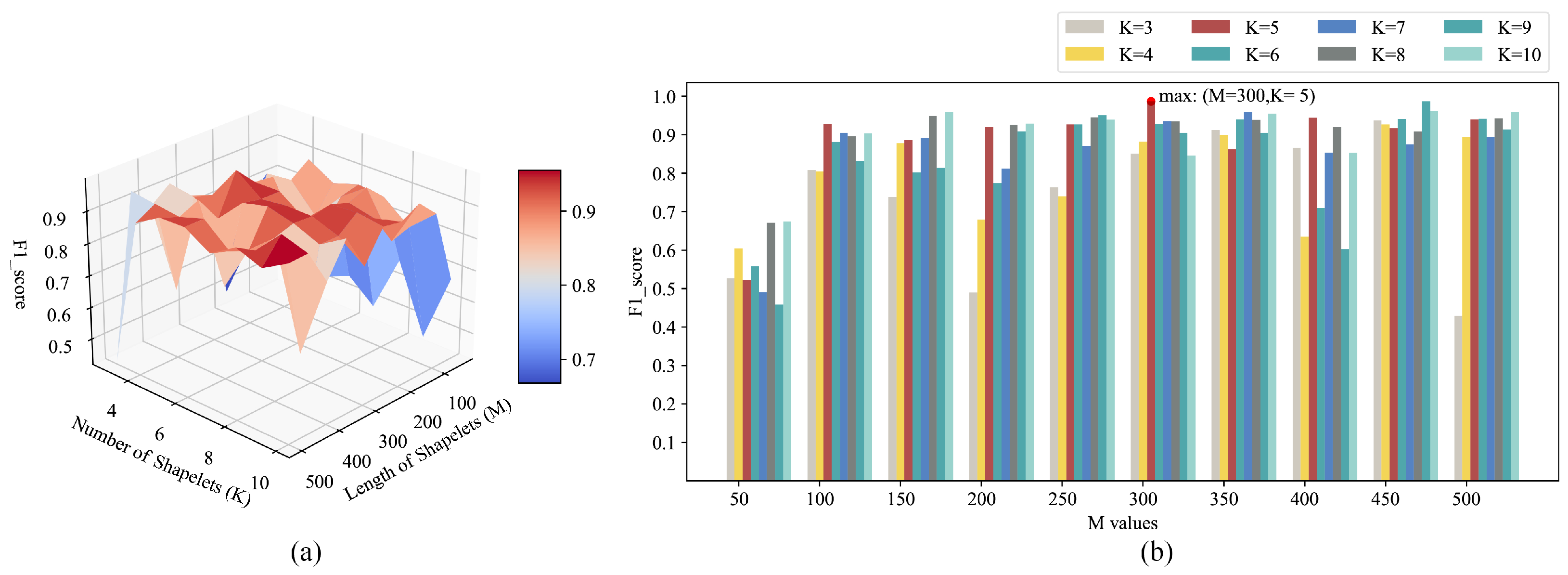
Firstly, we constrain the weights to be optimized in the feature extraction network so that they fall in the range of −1 to 1, which also limits the search range of the differential evolution algorithm. Then, in the first stage of model training, the learning rate of the SGD optimization method is set as 0.01. Furthermore, in the feature extraction network, there are two parameters that can directly affect the effectiveness of feature extraction: the length and number of shapelets, assuming that the length of shapelets is M and the number of shapelets is K. To find the appropriate parameter values, we conducted a grid search on and . Due to the fact that the F1 score can comprehensively consider precision and recall, which are important evaluation metrics in detecting LTE-R cells with degraded communication performance [3], the F1 score is used as the evaluation metric for the grid search. When conducting the grid search, an SVM is used to classify the training set after feature extraction. The average F1 score obtained from a 5-fold cross-validation is taken as the evaluation result for each search. The grid search results for M and K are shown in Figure 7.
It can be seen from Figure 7 that when M equals 300 and K equals 5, we can obtain the maximum F1 score value. Therefore, in this experiment, we set the length of the shapelets M to 300 and the number of shapelets to 5.
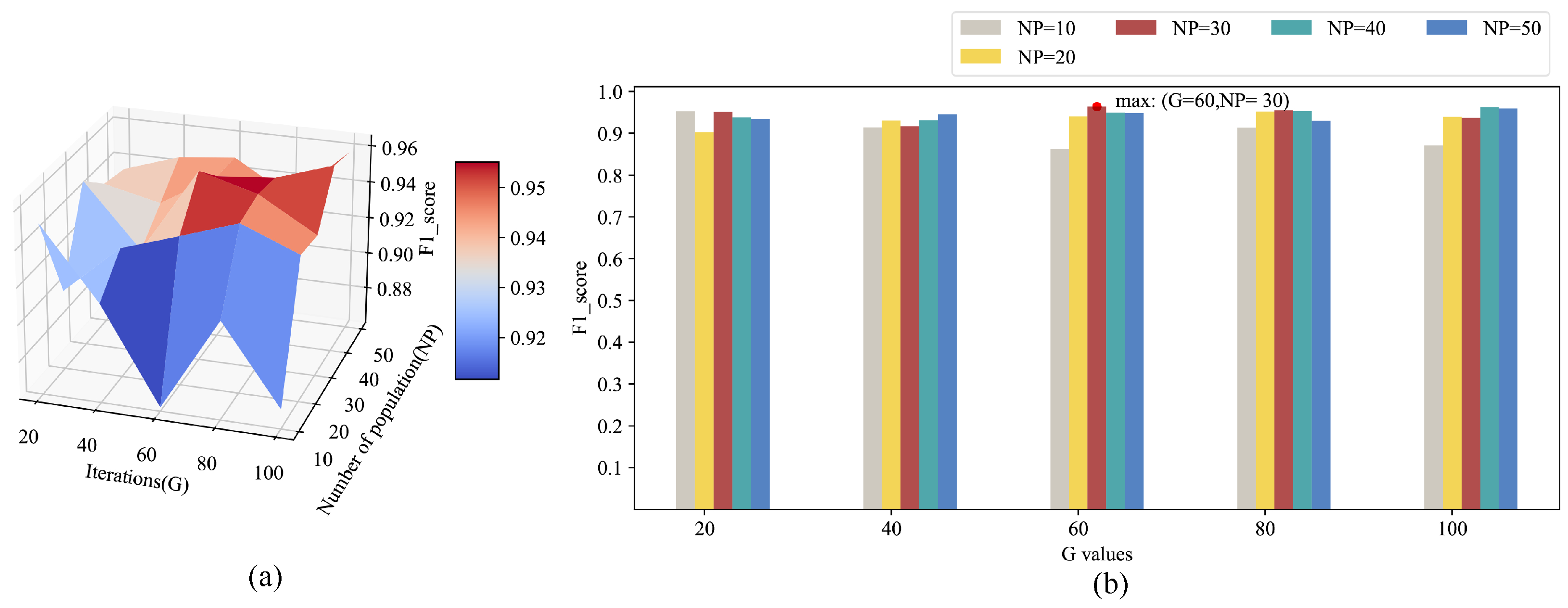
After determining the length and number of shapelets, it is necessary to determine the relevant parameters of the differential evolution algorithm in order to further ensure the performance of the detection method, i.e., the maximum iteration G and the population . Generally speaking, the larger the population size and maximum generation, the better the optimization effect. However, increasing G and can also lead to increased computational complexity, which affects algorithm efficiency. To find appropriate parameter values, we conduct a grid search on and . Similarly, we conduct a grid search and utilize an SVM to classify the training set after feature extraction. The average F1 score obtained from a 5-fold cross-validation is taken as the evaluation result for each search. The grid search results for G and are shown in Figure 8.
As can be seen from Figure 8, when equals 30 and G equals 60, we can obtain the maximum F1 score. Therefore, in this experiment, we set the population to 30 and the maximum iteration to 60.
All the codes of our approach and comparison methods are written in Python 3.6. All the experiments were carried out on a laptop, which was configured as follows: CPU is i5-8400 (Intel, Santa Clara, CA, USA), memory is 8G, and the graphics card is NIVIDA 1050Ti 4G (NIVIDA, Santa Clara, CA, USA).
5.3. Comparison and Discussion
In this section, comparative experiments on the detection dataset of LTE-R cells with degraded communication performance are presented in order to verify the performance of the method proposed in this paper. The experimental results are discussed and analyzed.
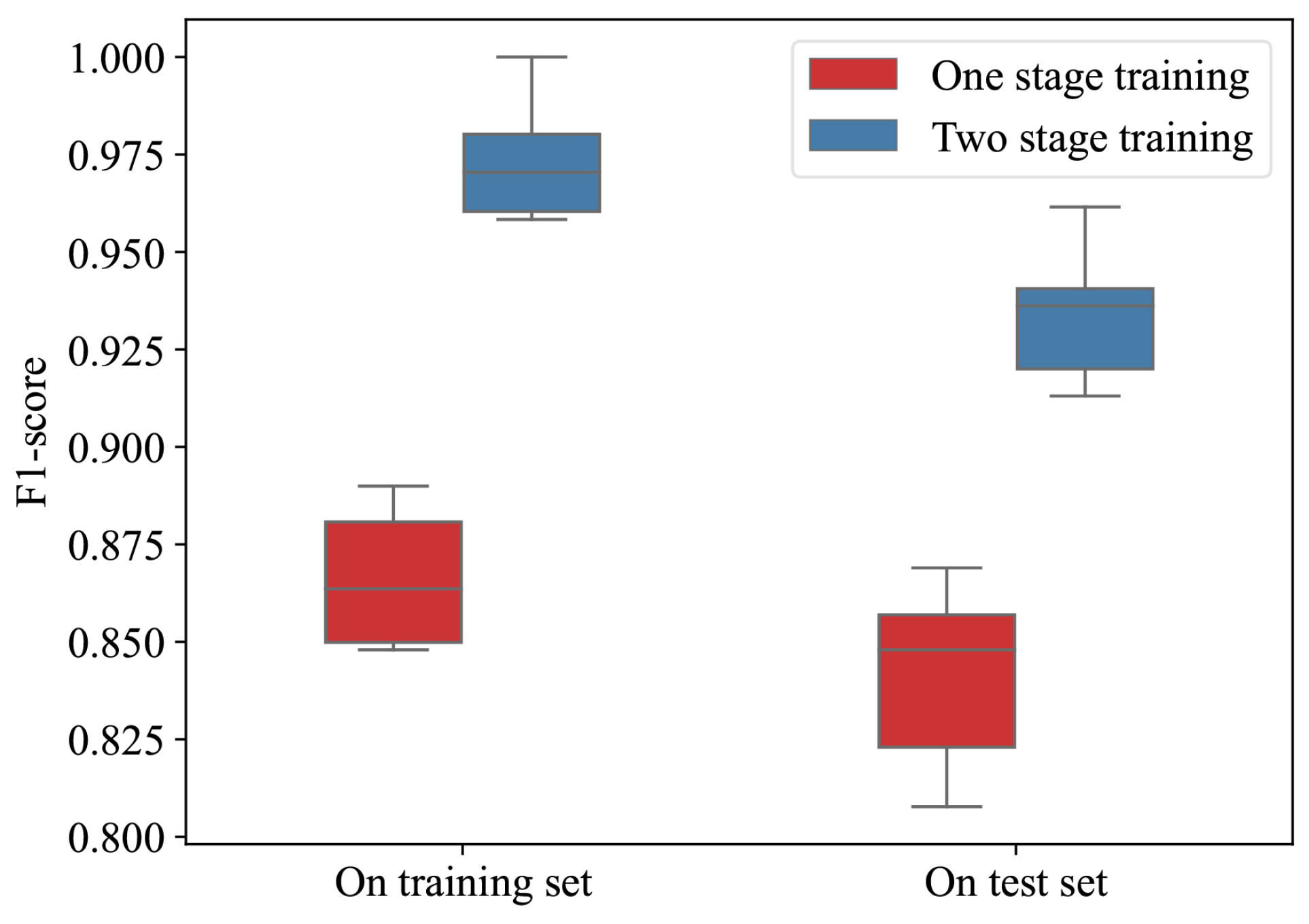
Before conducting the comparative experiments, we first verified the effectiveness of the proposed two-stage training method on the experimental dataset. Figure 9 illustrates the classification performance of the model after training it 10 times on the training and test sets, both with and without using the two-stage training method.
As can be seen from Figure 9, the two-stage training method proposed in this paper can significantly improve the training performance of the model compared to the training method that only uses contrastive loss and SGD (one-stage training). This is because the use of the differential evolution algorithm compensates for the deficiency of contrastive loss, which only focuses on between-class scatter.
When conducting the comparative experiments, several imbalanced data classification methods, such as SMOTE-SVM [41], ADASYM-SVM [41], Cosen-SVM [42], and several anomaly detection methods, such as LOF [7], VAE [14], and DEDAE [3] are selected as comparison methods. Considering that the detection of LTE-R cells with degraded communication performance is a sequence data classification problem, we also selected two sequence data classification approaches for performance comparison: the fast shapelet tree (FST) proposed by Rakthanmanon et al. [43] and the learning time series (LTS) proposed by Grabocka et al. [44]. Furthermore, considering the imbalance of the experimental data, a CNN-based imbalanced sequences classification approach, called the cost-sensitive convolution neural network (CSCNN) [26], was also selected as a comparison approach.
To verify the effectiveness of the proposed approach for feature extraction, we designed experiments to compare the feature extraction capabilities. Figure 10 shows the distribution of features extracted by our approach, FST, LTS, CSCNN, VAE, and DEDAE on the degradation detection dataset in the feature space.
Figure 10 illustrates the feature data after PCA dimensionality reduction. It can be seen that the features extracted by the proposed feature extraction neural network were able to distinguish between normal and abnormal cells at the feature level. This is because the proposed optimization objective, based on the Fisher criterion, can minimize the within-class scatter of extracted features while maximizing the between-class scatter. The features extracted by the other five comparison approaches could not clearly distinguish between the two types of samples at the feature level, which affected the accuracy of classification. The experiments showed that the proposed approach has obvious advantages over the comparison approaches when extracting imbalanced sequence features.
Then, in order to verify the classification performance of the proposed approach, we compared the classification performance of our model to baselines on the degradation detection dataset. The evaluation metrics for classification performance include G-mean, AUC, F1 score, and precision. The calculation process of each evaluation metric can be found in [45]. During the experiments, each approach trained the model on the training set and used the trained model to calculate the various evaluation metrics on the test set. After repeating the above process five times, we could obtain the mean and standard deviation of the different evaluation metrics for each approach. Table 4 shows the classification performance of each approach on the degradation detection dataset.
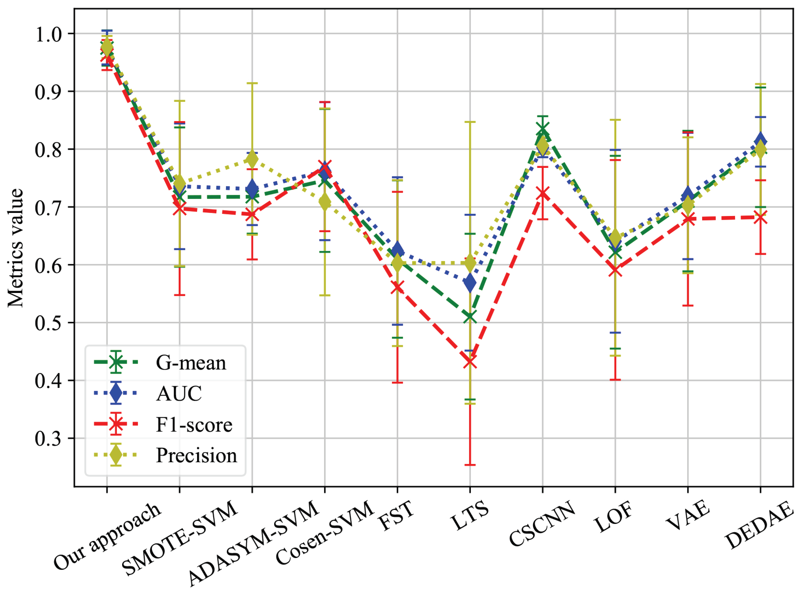
In order to compare the classification performance of the comparison approaches on the degradation detection dataset more intuitively, Figure 11 shows the performance of each approach on different evaluation metrics.
As can be seen from Figure 10 and Figure 11, our approach was significantly superior to all other comparison approaches in terms of G-mean, AUC, F1 score, and precision. CSCNN also achieved good results, which can be attributed to its use of cost-sensitive loss functions and the strong feature extraction ability of convolutional networks for sequence data. However, CSCNN still had a significant disadvantage compared to our approach due to the difficulty in determining cost-sensitive factors. The imbalanced data classification methods and anomaly detection methods also showed relatively good performance. However, as can be seen from Figure 11, these methods were significantly less stable than our approach. FST and LTS performed the worst due to the insufficient information provided by the minority class samples, resulting in model bias.
From the above experiments, it can be seen that the imbalanced sequence feature extraction neural network proposed in this paper has excellent performance for the detection of LTE-R cells with degraded communication performance. Our approach can achieve an accuracy of about 98% on various imbalanced data classification evaluation metrics, which provides good decision support for the operation and maintenance of the Shuo Huang Railway LTE-R communication network.
6. Conclusions
In order to solve the problem of detecting LTE-R cells with degraded communication performance in the Shuo Huang Railway, we designed a deep neural network structure that can achieve imbalanced sequence feature extraction based on the CNN network structure and the idea of shapelet transformation. Then, considering the imbalance between the numbers of degraded cell samples and normal cell samples, the optimization objective of the imbalanced sequence feature extraction neural network was designed based on the Fisher criterion. Afterward, in order to determine the appropriate weights of the feature extraction network, we developed a two-stage training method. In the first stage, we used SGD and contrastive loss to preliminarily train the model. In the second stage, we used the differential evolution algorithm to further optimize the weights of the distance calculation layer. Finally, based on the sequences of key performance indicators from the drive test data for each Shuo Huang Railway LTE-R cell, as well as the corresponding EARR data, we constructed a degradation detection dataset and conducted experiments on this dataset using the proposed approach and other comparison approaches. The experimental results show that the proposed feature extraction network could effectively extract the features of imbalanced sequences and that its classification performance was significantly better than that of the other comparison approaches. The proposed approach achieved an accuracy of 98% or above in detecting LTE-R cells with degraded communication performance, which means that it could be a powerful tool for the operation and maintenance of the Shuo Huang Railway LTE-R network and has high application value.
Author Contributions
Conceptualization, J.Q. and H.M.; methodology, J.Q.; software, J.Q.; investigation, J.Q. and H.M.; resources, J.Q.; data curation, J.Q.; writing—original draft preparation, J.Q. and H.M.; writing—review and editing, J.Q., H.M. and C.Q.; visualization, J.Q.; supervision, C.Q.; project administration, J.Q. All authors have read and agreed to the published version of the manuscript.
Funding
This work is supported by the Key Scientific and Technological Project of Henan Province (no. 222102210006) and the Science and Technology Development Project of China Railway Design Corporation (no. 2022A02538005).
Data Availability Statement
The data can be shared up on request and the data are not publicly available due to information security issues.
Conflicts of Interest
Jiantao Qu, Chunyu Qi and He Meng are employees of China Railway Design Corporation (China) Company. The authors declare no conflicts of interest regarding the publication of this research article.
References
- Li, Y.; Meng, Z. Design and implementation of a coal-dust removal device for heavy-haul railway tunnels. Transp. Saf. Environ. 2020, 2, 283–291. [Google Scholar] [CrossRef]
- Qu, J.; Liu, F.; Ma, Y.; Fan, J. Temporal-spatial Collaborative Prediction for LTE-R Communication Quality Based on Deep Learning. IEEE Access 2020, 8, 94817–94832. [Google Scholar] [CrossRef]
- Qu, J.; Liu, F.; Ma, Y. A dual encoder DAE neural network for imbalanced binary classification based on NSGA-3 and GAN. Pattern Anal. Appl. 2022, 25, 17–34. [Google Scholar] [CrossRef]
- Chernogorov, F.; Ristaniemi, T.; Brigatti, K.; Chernov, S. N-gram analysis for sleeping cell detection in LTE networks. In Proceedings of the International Conference on Acoustics, Speech and Signal Processing, Vancouver, BC, Canada, 26–31 May 2013. [Google Scholar]
- Chernov, S.; Cochez, M.; Ristaniemi, T. Anomaly detection algorithms for the sleeping cell detection in LTE networks. In Proceedings of the 2015 IEEE 81st Vehicular Technology Conference (VTC Spring), Glasgow, UK, 11–14 May 2015; IEEE: Piscataway, NJ, USA, 2015; pp. 1–5. [Google Scholar]
- Miao, D.; Qin, X.; Wang, W. Anomalous cell detection with kernel density-based local outlier factor. China Commun. 2015, 12, 64–75. [Google Scholar] [CrossRef]
- Safaei, M.; Ismail, A.S.; Chizari, H.; Driss, M.; Boulila, W.; Asadi, S.; Safaei, M. Standalone noise and anomaly detection in wireless sensor networks: A novel time-series and adaptive Bayesian-network-based approach. Softw. Pract. Exp. 2020, 50, 428–446. [Google Scholar] [CrossRef]
- Premkumar, M.; Sundararajan, T. DLDM: Deep learning-based defense mechanism for denial of service attacks in wireless sensor networks. Microprocess. Microsyst. 2020, 79, 103278. [Google Scholar] [CrossRef]
- Regin, R.; Rajest, S.; Singh, B. Fault detection in wireless sensor network based on deep learning algorithms. EAI Endorsed Trans. Scalable Inf. Syst. 2021, 8, e8. [Google Scholar] [CrossRef]
- Kuadey, N.A.E.; Maale, G.T.; Kwantwi, T.; Sun, G.; Liu, G. DeepSecure: Detection of distributed denial of service attacks on 5G network slicing—Deep learning approach. IEEE Wirel. Commun. Lett. 2021, 11, 488–492. [Google Scholar] [CrossRef]
- Aljebreen, M.; Alrayes, F.S.; Maray, M.; Aljameel, S.S.; Salama, A.S.; Motwakel, A. Modified Equilibrium Optimization Algorithm with Deep Learning-Based DDoS Attack Classification in 5G Networks. IEEE Access 2023, 11, 108561–108570. [Google Scholar] [CrossRef]
- Dahiya, D. DDoS attacks detection in 5G networks: Hybrid model with statistical and higher-order statistical features. Cybern. Syst. 2023, 54, 888–913. [Google Scholar] [CrossRef]
- Aghbashlo, M.; Peng, W.; Tabatabaei, M.; Kalogirou, S.A.; Soltanian, S.; Hosseinzadeh-Bandbafha, H.; Mahian, O.; Lam, S.S. Machine learning technology in biodiesel research: A review. Prog. Energy Combust. Sci. 2021, 85, 100904. [Google Scholar] [CrossRef]
- Huan, W.; Lin, H.; Lie, H.; Zhou, Y.; Wang, Y. Anomaly Detection Method Based On Clustering Undersampling And Ensemble Learning. Space Sci. Technol. 2020, 2022, 980–984. [Google Scholar]
- Jing, X.Y.; Zhang, X.; Zhu, X.; Wu, F.; You, X.; Gao, Y.; Shan, S.; Yang, J.Y. Multiset feature learning for highly imbalanced data classification. IEEE Trans. Pattern Anal. Mach. Intell. 2019, 43, 139–156. [Google Scholar] [CrossRef] [PubMed]
- Phua, C.; Alahakoon, D.; Lee, V. Minority report in fraud detection: Classification of skewed data. ACM SIGKDD Explor. Newsl. 2004, 6, 50–59. [Google Scholar] [CrossRef]
- Laurikkala, J. Instance-based data reduction for improved identification of difficult small classes. Intell. Data Anal. 2002, 6, 311–322. [Google Scholar] [CrossRef]
- Farshidvard, A.; Hooshmand, F.; MirHassani, S. A novel two-phase clustering-based under-sampling method for imbalanced classification problems. Expert Syst. Appl. 2023, 213, 119003. [Google Scholar] [CrossRef]
- Han, H.; Wang, W.Y.; Mao, B.H. Borderline-SMOTE: A new over-sampling method in imbalanced data sets learning. In Proceedings of the International Conference on Intelligent Computing, Hefei China, 23–26 August 2005; Springer: Berlin/Heidelberg, Germany, 2005; pp. 878–887. [Google Scholar]
- He, H.; Bai, Y.; Garcia, E.A.; Li, S. ADASYN: Adaptive synthetic sampling approach for imbalanced learning. In Proceedings of the 2008 IEEE International Joint Conference on Neural Networks (IEEE World Congress on Computational Intelligence), Hong Kong, China, 1–8 June 2008; IEEE: Piscataway, NJ, USA, 2008; pp. 1322–1328. [Google Scholar]
- Islam, A.; Belhaouari, S.B.; Rehman, A.U.; Bensmail, H. KNNOR: An oversampling technique for imbalanced datasets. Appl. Soft Comput. 2022, 115, 108288. [Google Scholar] [CrossRef]
- Khreich, W.; Khosravifar, B.; Hamou-Lhadj, A.; Talhi, C. An anomaly detection system based on variable N-gram features and one-class SVM. Inf. Softw. Technol. 2017, 91, 186–197. [Google Scholar] [CrossRef]
- Wang, K.; An, J.; Yu, Z.; Yin, X.; Ma, C. Kernel local outlier factor-based fuzzy support vector machine for imbalanced classification. Concurr. Comput. Pract. Exp. 2021, 33, e6235. [Google Scholar] [CrossRef]
- Zhang, X.; Yao, Y.; Lv, C.; Wang, T. Anomaly credit data detection based on enhanced Isolation Forest. Int. J. Adv. Manuf. Technol. 2022, 122, 185–192. [Google Scholar] [CrossRef]
- Zhang, C.; Tan, K.C.; Li, H.; Hong, G.S. A cost-sensitive deep belief network for imbalanced classification. IEEE Trans. Neural Netw. Learn. Syst. 2018, 30, 109–122. [Google Scholar] [CrossRef] [PubMed]
- Geng, Y.; Luo, X. Cost-sensitive convolutional neural networks for imbalanced time series classification. Intell. Data Anal. 2019, 23, 357–370. [Google Scholar] [CrossRef]
- An, J.; Cho, S. Variational autoencoder based anomaly detection using reconstruction probability. Spec. Lect. IE 2015, 2, 1–18. [Google Scholar]
- Schlegl, T.; Seeböck, P.; Waldstein, S.M.; Schmidt-Erfurth, U.; Langs, G. Unsupervised anomaly detection with generative adversarial networks to guide marker discovery. In Proceedings of the International Conference on Information Processing in Medical Imaging, Boone, NC, USA, 25–30 June 2017; Springer: Cham, Switzerland, 2017; pp. 146–157. [Google Scholar]
- Cheng, Z.; Wang, S.; Zhang, P.; Wang, S.; Liu, X.; Zhu, E. Improved autoencoder for unsupervised anomaly detection. Int. J. Intell. Syst. 2021, 36, 7103–7125. [Google Scholar] [CrossRef]
- Wang, Z.; Peng, C.; Zhang, Y.; Wang, N.; Luo, L. Fully convolutional siamese networks based change detection for optical aerial images with focal contrastive loss. Neurocomputing 2021, 457, 155–167. [Google Scholar] [CrossRef]
- Jiao, Y.; Yang, K.; Song, D.; Tao, D. Timeautoad: Autonomous anomaly detection with self-supervised contrastive loss for multivariate time series. IEEE Trans. Netw. Sci. Eng. 2022, 9, 1604–1619. [Google Scholar] [CrossRef]
- Oproiu, M.; Boldan, V.; Marghescu, I. Effects of using carrier aggregation with three component carriers in a mobile operator’s network. In Proceedings of the 2016 International Conference on Communications (COMM), Bucharest, Romania, 9–10 June 2016; IEEE: Piscataway, NJ, USA, 2016; pp. 169–172. [Google Scholar]
- Ye, L.; Keogh, E. Time series shapelets: A new primitive for data mining. In Proceedings of the 15th ACM SIGKDD International Conference on Knowledge Discovery and Data Mining, Paris, France, 28 June–1 July 2009; pp. 947–956. [Google Scholar]
- Chen, T.; Luo, C.; Li, L. Intriguing properties of contrastive losses. Adv. Neural Inf. Process. Syst. 2021, 34, 11834–11845. [Google Scholar]
- Li, Z.; Liu, F.; Yang, W.; Peng, S.; Zhou, J. A survey of convolutional neural networks: Analysis, applications, and prospects. IEEE Trans. Neural Netw. Learn. Syst. 2021, 33, 6999–7019. [Google Scholar] [CrossRef]
- Fisher, R.A. The use of multiple measurements in taxonomic problems. Ann. Eugen. 1936, 7, 179–188. [Google Scholar] [CrossRef]
- Pant, M.; Zaheer, H.; Garcia-Hernandez, L.; Abraham, A. Differential Evolution: A review of more than two decades of research. Eng. Appl. Artif. Intell. 2020, 90, 103479. [Google Scholar]
- Gao, S.; Wang, K.; Tao, S.; Jin, T.; Dai, H.; Cheng, J. A state-of-the-art differential evolution algorithm for parameter estimation of solar photovoltaic models. Energy Convers. Manag. 2021, 230, 113784. [Google Scholar] [CrossRef]
- Singh, D.; Kaur, M.; Jabarulla, M.Y.; Kumar, V.; Lee, H.N. Evolving fusion-based visibility restoration model for hazy remote sensing images using dynamic differential evolution. IEEE Trans. Geosci. Remote Sens. 2022, 60, 1–14. [Google Scholar] [CrossRef]
- Ren, L.; Zhao, D.; Zhao, X.; Chen, W.; Li, L.; Wu, T.; Liang, G.; Cai, Z.; Xu, S. Multi-level thresholding segmentation for pathological images: Optimal performance design of a new modified differential evolution. Comput. Biol. Med. 2022, 148, 105910. [Google Scholar] [CrossRef] [PubMed]
- Ramadhan, N.G. Comparative Analysis of ADASYN-SVM and SMOTE-SVM Methods on the Detection of Type 2 Diabetes Mellitus. Sci. J. Inform. 2021, 8, 276–282. [Google Scholar] [CrossRef]
- Iranmehr, A.; Masnadi-Shirazi, H.; Vasconcelos, N. Cost-sensitive support vector machines. Neurocomputing 2019, 343, 50–64. [Google Scholar] [CrossRef]
- Rakthanmanon, T.; Keogh, E. Fast shapelets: A scalable algorithm for discovering time series shapelets. In Proceedings of the 2013 SIAM International Conference on Data Mining, Austin, TX, USA, 2–4 May 2013; SIAM: Philadelphia, PA, USA, 2013; pp. 668–676. [Google Scholar]
- Grabocka, J.; Schilling, N.; Wistuba, M.; Schmidt-Thieme, L. Learning time-series shapelets. In Proceedings of the 20th ACM SIGKDD International Conference on Knowledge Discovery and Data Mining, New York, NY, USA, 24–27 August 2014; pp. 392–401. [Google Scholar]
- Hemalatha, P.; Amalanathan, G.M. FG-SMOTE: Fuzzy-based Gaussian synthetic minority oversampling with deep belief networks classifier for skewed class distribution. Int. J. Intell. Comput. Cybern. 2021, 14, 270–287. [Google Scholar] [CrossRef]
Figure 1.
The source of Shuo Huang Railway operation and maintenance data.

Figure 2.
The construction process of the dataset for the detection of LTE-R cells with degraded communication performance.
Figure 2.
The construction process of the dataset for the detection of LTE-R cells with degraded communication performance.

Figure 3.
The overall framework of the proposed approach.

Figure 4.
The working principle of min pooling.

Figure 5.
The basic principle of Fisher criterion.

Figure 6.
The flow of the two-stage training method.

Figure 7.
The grid search results of M and K. (a) shows the grid search results for K and M in the form of a heat map, and the darker the color, the higher the F1 score. (b) shows the grid search results for K and M in the form of a group bar chart, and the longer the length of the bar, the higher the F1 score.

Figure 8.
The grid search results of G and . (a) shows the grid search results for G and NP in the form of a heat map, and the darker the color, the higher the F1 score. (b) shows the grid search results for G and NP in the form of a group bar chart, and the longer the length of the bar, the higher the F1 score.

Figure 9.
Comparison of different training methods.

Figure 10.
The performance comparison of feature extraction.

Figure 11.
Performance of each approach on different evaluation metrics.


Table 1.
QCI value and its corresponding services.
| Terminal Type | Communication Service | QCI Value |
|---|---|---|
| Terminal of train operation control | Train control data transmission service | 1 |
| Emergency call | 1 | |
| The cab-integrated radio communication equipment | Transmission dispatching order | 2 |
| Wireless train number calibration | 2 | |
| In-vehicle speech | 2 | |
| Handheld mobile station | Emergency call | 1 |
| Speech call | 3 | |
| Train video surveillance system | Video Surveillance | 4 |
Table 2.
The structure of the feature extraction neural network.
| Layer Type | Input Shape | Output Shape |
|---|---|---|
| Input layer | (None, 500, 1) | (None, 500, 1) |
| 1D convolutional layer | (None, 500, 1) | (None, 101, 400) |
| Squared distance layer | (None, 101, 400) | (None, 101, 7) |
| Min pooling layer | (None, 101, 7) | (None, 7) |
Table 3.
The detailed information of the degradation detection dataset.
| Data Properties | Property Values |
|---|---|
| Sequence length | 500 |
| Dataset size | 2554 |
| Normal data size | 2470 |
| Abnormal data size | 84 |
| Training set size | 1788 |
| Test set size | 766 |
| Imbalance ratio | 29.4 |
Table 4.
The classification results of each approach.
| Name | G-Mean | AUC | F1 Score | Precision |
|---|---|---|---|---|
| SMOTE-SVM | 0.7194 ± 0.1048 | 0.7238 ± 0.1079 | 0.7041 ± 0.1194 | 0.6862 ± 0.1028 |
| ADASYM-SVM | 0.7063 ± 0.1035 | 0.7095 ± 0.1066 | 0.6919 ± 0.1195 | 0.6595 ± 0.0857 |
| Cosen-SVM | 0.6835 ± 0.1360 | 0.6929 ± 0.1339 | 0.6658 ± 0.1637 | 0.6483 ± 0.1385 |
| FST | 0.5231 ± 0.0058 | 0.5333 ± 0.005 | 0.4788 ± 0.0009 | 0.501 ± 0.0026 |
| LTS | 0.5294 ± 0.0001 | 0.5292 ± 0.0001 | 0.5262 ± 0.0087 | 0.5195 ± 0.0007 |
| CSCNN | 0.8448 ± 0.0332 | 0.8564 ± 0.0277 | 0.7439 ± 0.0263 | 0.7741 ± 0.0309 |
| LOF | 0.6217 ± 0.1667 | 0.6405 ± 0.158 | 0.5911 ± 0.19 | 0.6467 ± 0.204 |
| VAE | 0.7101 ± 0.1215 | 0.719 ± 0.1093 | 0.6793 ± 0.1499 | 0.7029 ± 0.1175 |
| DEDAE | 0.8032 ± 0.1034 | 0.8126 ± 0.0428 | 0.6824 ± 0.0637 | 0.7994 ± 0.1132 |
| Our approach | 0.9863 ± 0.0092 | 0.9864 ± 0.0091 | 0.9799 ± 0.0004 | 0.9872 ± 0.0181 |
Disclaimer/Publisher’s Note: The statements, opinions and data contained in all publications are solely those of the individual author(s) and contributor(s) and not of MDPI and/or the editor(s). MDPI and/or the editor(s) disclaim responsibility for any injury to people or property resulting from any ideas, methods, instructions or products referred to in the content. |
© 2024 by the authors. Licensee MDPI, Basel, Switzerland. This article is an open access article distributed under the terms and conditions of the Creative Commons Attribution (CC BY) license (https://creativecommons.org/licenses/by/4.0/).
Share and Cite
MDPI and ACS Style
Qu, J.; Qi, C.; Meng, H. An Imbalanced Sequence Feature Extraction Approach for the Detection of LTE-R Cells with Degraded Communication Performance. Future Internet 2024, 16, 30. https://doi.org/10.3390/fi16010030
AMA Style
Qu J, Qi C, Meng H. An Imbalanced Sequence Feature Extraction Approach for the Detection of LTE-R Cells with Degraded Communication Performance. Future Internet. 2024; 16(1):30. https://doi.org/10.3390/fi16010030
Chicago/Turabian StyleQu, Jiantao, Chunyu Qi, and He Meng. 2024. "An Imbalanced Sequence Feature Extraction Approach for the Detection of LTE-R Cells with Degraded Communication Performance" Future Internet 16, no. 1: 30. https://doi.org/10.3390/fi16010030
Note that from the first issue of 2016, this journal uses article numbers instead of page numbers. See further details here.