Diff-SwinT: An Integrated Framework of Diffusion Model and Swin Transformer for Radar Jamming Recognition

Abstract

With the increasing complexity of radar jamming threats, accurate and automatic jamming recognition is essential but remains challenging. Conventional algorithms often suffer from sharply decreased recognition accuracy under low jamming-to-noise ratios (JNR).Artificial intelligence-based jamming signal recognition is currently the main research directions for this issue. This paper proposes a new radar jamming recognition framework called Diff-SwinT. Firstly, the time-frequency representations of jamming signals are generated using Choi-Williams distribution. Then, a diffusion model with U-Net backbone is trained by adding Gaussian noise in the forward process and reconstructing in the reverse process, obtaining an inverse diffusion model with denoising capability. Next, Swin Transformer extracts hierarchical multi-scale features from the denoised time-frequency plots, and the features are fed into linear layers for classification. Experiments show that compared to using Swin Transformer, the proposed framework improves overall accuracy by 15% to 10% at JNR from −16 dB to −8 dB, demonstrating the efficacy of diffusion-based denoising in enhancing model robustness. Compared to VGG-based and feature-fusion-based recognition methods, the proposed framework has over 27% overall accuracy advantage under JNR from −16 dB to −8 dB. This integrated approach significantly enhances intelligent radar jamming recognition capability in complex environments.

1. Introduction

Radar systems serve as the eyes and ears of modern armed forces, providing vital intelligence for situational awareness, target tracking, and threat detection. In electronic warfare, adversaries employ various jamming signals to degrade radar detection, tracking, and guidance capabilities [1,2]. For example, in air defense systems, jamming can disrupt tracking of aircraft and missiles, making it difficult to detect and intercept threats. Shipborne radars for surface surveillance are also susceptible to jamming, which can cloak naval vessels and enable attacks [3,4]. The emergence of Digital Radio Frequency Memory (DRFM) systems has ushered in a new era for active radar jamming techniques, enabling adversaries to generate various jamming modes and making the effective operation of radar systems increasingly challenging. By identifying the jamming type, radar can invoke tailored anti-jamming techniques like sidelobe cancellation, increased power, or frequency hopping to mitigate the jamming effects [5,6]. Therefore, accurate recognition of jamming signals is an essential step for radar systems to take appropriate countermeasures and maintain operational effectiveness under jamming [7,8,9].

Various techniques have been developed for radar jamming recognition over the years. Earlier methods rely on expert-crafted features based on signal processing concepts like frequency entropy and peak-to-peak ratio [10]. These hand-engineered features provide interpretable insights into jamming characteristics. However, these hand-engineered features often fail to capture subtle jamming patterns, especially at low jamming-to-noise ratios (JNRs) [11].The predefined features lack sufficient representation power to discern fine-grained differences when the signal is corrupted by noise. With the rise of deep learning, artificial intelligence-based data-driven approaches using convolutional neural networks (CNNs) have achieved new benchmarks. By automatically learning features from data, CNNs can extract intricate discriminative patterns without expert domain knowledge. Methods based on time-frequency representations and complex CNNs can attain over 95% accuracy on measured data [12,13,14,15]. Advanced networks incorporating long short-term memory units [16,17,18], attention mechanisms [19,20], and pruning [21] further boost performance. For example, Lin et al. combined Fisher pruning and complex networks to achieve excellent accuracy even on low-resource devices [22,23,24]. Recent works also apply deep learning to large-scale collected data, obtaining promising results in real-world jamming recognition [25]. However, despite remarkable recognition accuracy under high JNRs, existing methods still face difficulties in discerning jamming types under low JNRs like −18 dB [26]. Adversarial attacks can also degrade CNN performance [27,28,29,30], posing challenges for deep learning based recognition.

Despite promising results, existing methods still face difficulties in jamming recognition under low JNRs. Most methods can achieve over 90% accuracy when JNR is above −6 dB [31,32,33,34]. However, their performance deteriorates rapidly at even lower JNRs. Low JNR poses great challenges for subtle feature extraction. First, convolutional kernels for extracting image features of the jamming signal tend to focus on local patterns, whereas attention mechanisms are better suited to capture global contextual features. Second, strong background noise can drown out parts of the meaningful signal, requiring active denoising interventions to reverse this effect. Robust feature learning and selection are thus needed to address the low JNR jamming recognition problem from both perspectives [35,36]. Advanced network architectures and noise-robust feature extraction need to be explored to enable accurate jamming recognition in complex noisy environments. Tackling the low JNR challenge will greatly extend the capability of radar systems against jamming attacks.

In recent years, diffusion models have gained widespread attention in image generation and restoration. Unlike traditional denoising autoencoders, diffusion models progressively model the data by adding noise through a forward process, then reverse this process via a carefully designed denoising procedure to achieve high-quality sample generation [37,38,39]. This model architecture endows diffusion models with powerful capabilities in image restoration and denoising. By employing diffusion models as a preprocessing module, the subsequent model’s denoising performance can be effectively improved.

Meanwhile, vision transformers have also been advancing rapidly. Compared to convolutional networks, transformers can model long-range dependencies via the self-attention mechanism and capture information from different representational subspaces through multi-head self-attention [40]. Swin Transformer (SwinT) reduces the computational and memory costs substantially through the shifted window attention design and hierarchical representation [41,42]. It is one of the important advancements in vision transformer architectures. Since radar jamming signal time-frequency graphs contain relatively complex global patterns, using SwinT can better learn their global feature representations and boost jamming recognition performance.

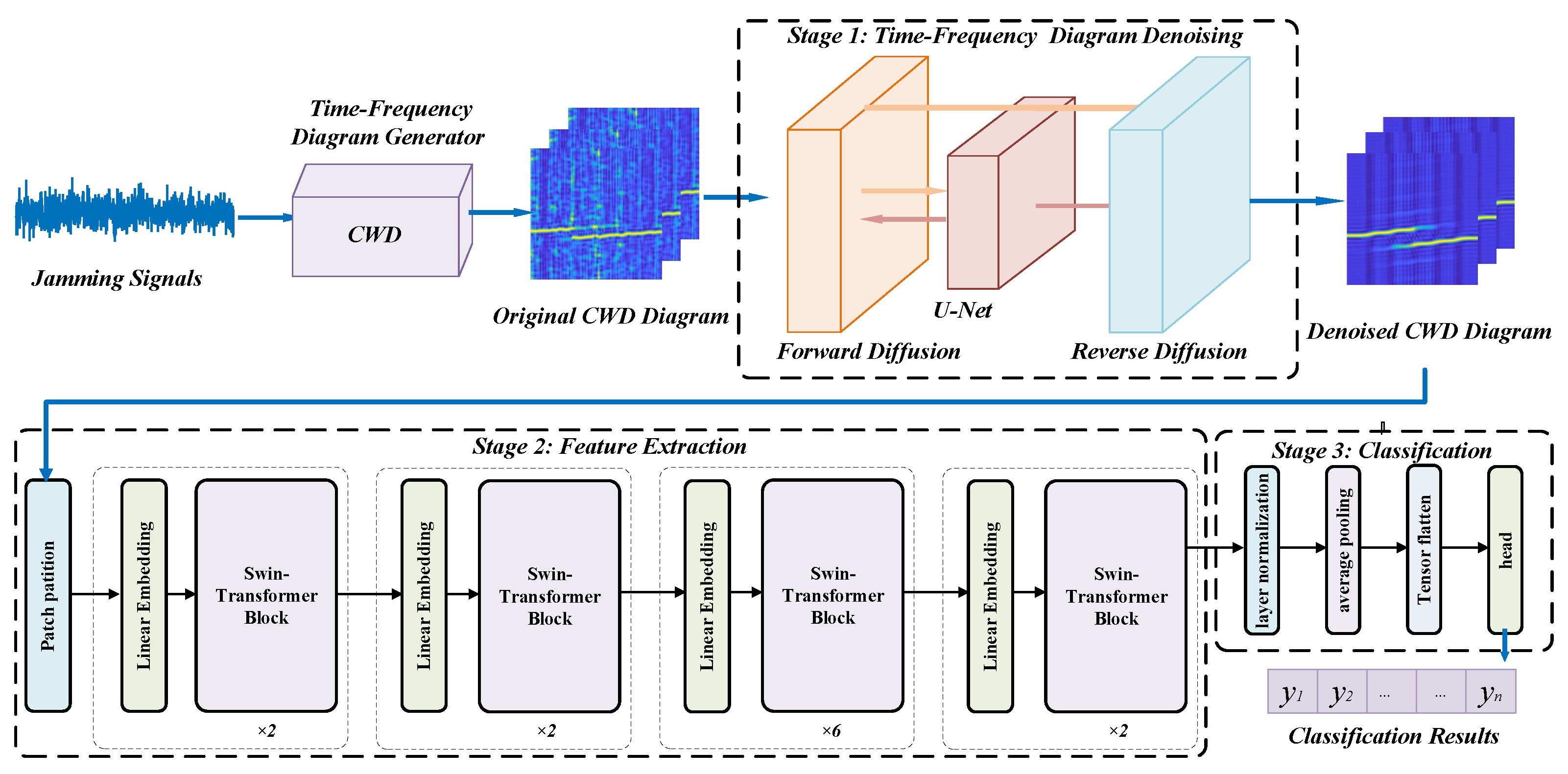
This paper proposes using diffusion models as the preprocessing module to denoise the input signals, then utilizing SwinT to extract global features from the time-frequency graphs, in order to further improve radar jamming recognition capabilities. The combination of these two models provides new insights for jamming recognition in complex scenarios.The overall framework of the proposed method is shown in Figure 1.

This paper first establishes mathematical models for 8 common radar jamming patterns in Section 2, providing the basis for subsequent analyses and experiments. Section 3 then proposes a novel jamming recognition framework integrating multiple techniques including CWD time-frequency graph representation, diffusion models for denoising, SwinT for feature extraction, and customized loss functions. Simulations and experiments are conducted in Section 4 to demonstrate the effectiveness and robustness of the proposed method under various conditions. Finally, Section 5 summarizes the critical innovations and contributions of this work.

2. Radar Jamming Signal Analysis and Modeling

2.1. Noise Modulation Jamming

Noise modulation jamming typically utilizes noise signals to modulate certain parameters of the jamming signal. These techniques involve high transmission power, enabling the generated signals to effectively jam the target echo signal at the radar receiver, thus preventing the radar from performing its normal detection functions [43,44,45]. This paper primarily introduces two types of noise modulation jamming: Amplitude Modulation (AM) and Frequency Modulation (FM).

2.1.1. Noise Amplitude Modulation Jamming

Noise Amplitude Modulation Jamming (NAMJ) is a targeting technique that is both technically simple and popular on the electronic warfare battlefield. It involves modulating Gaussian white noise within the bandwidth of a radar’s linear frequency modulated signal. In other words, it utilizes high-powered modulated noise to suppress the radar signal within a specific frequency band, thus affecting the receiver’s ability to detect the signal. This method yields effective jamming results and is relatively straightforward to execute. However, due to its narrowband nature, it is unsuitable for conducting broad-spectrum jamming. The mathematical model for NAMJ is expressed as follows:

$$J\left(t\right)=\left[U_0+K_{AM}{U}_n\left(t\right)\right]\exp \left({\omega }_j+\phi \right)$$

(1)

The function expression is a generalized stationary random process, where $\exp \left(·\right)$ denotes the exponential function with the base e, $U_n\left(t\right)$ represents zero-mean Gaussian white noise, $U_0$ stands for the carrier voltage, and the modulation coefficient of the noise, $K_{AM}$, controls the power of $U_n\left(t\right)$. The interfering carrier phase ${\omega }_j$, representing the phase $\phi$ of the jamming, is uniformly distributed in the range $\left[0,2\pi \right]$ and is independent of $U_n\left(t\right)$.

2.1.2. Noise Frequency Modulation Jamming

Noise Frequency Modulation Jamming (NFMJ) is a form of broadband jamming commonly employed to disrupt frequency-diverse and frequency-agile radar systems.

$$J\left(t\right)=U_j\exp \left[j\left(2\pi f_c+2\pi K_{FM}\underset{0}{\overset{t}{\int }}u\left(t^{\prime }\right)d{t}^{\prime }+\phi \right)dt\right]$$

(2)

NFMJ is a generalized stationary random process, where $\exp \left(·\right)$ represents the exponential function with base e. The modulating noise $\phi$ is zero-mean Gaussian white noise, uniformly distributed within the range $\left[0,2\pi \right]$, and is independent of the signal $u\left(t\right)$. The carrier frequency $f_c$ is the central frequency of the noise frequency modulated signal. The modulation slope $K_{FM}$ determines the rate of frequency change. The amplitude $U_j$ of the jamming controls the increase or decrease of frequency caused by the intensity of the modulating signal. The effective modulation index $m_f$ can be calculated using the following equation:

$$m_f=K_{FM}/\Delta F_n$$

(3)

where $\Delta F_n$ represents the bandwidth of the modulating noise. The effective modulation index is a crucial determinant between coherent jamming and broadband jamming. When $m_f\ge 1$, the noise frequency modulation jamming transitions into broadband jamming; otherwise, it remains a coherent jamming technique.

2.2. Smart Noise Jamming

With the continuous advancement of radar technology, radar’s resistance to jamming has been steadily improving. Utilizing simple noise for suppression-style jamming doesn’t yield high energy efficiency and offers limited benefits. Simultaneously, the widespread adoption of sidelobe cancellation and nulling techniques has made it difficult for interfering signals to penetrate sidelobes, thereby increasing the difficulty of implementing traditional noise modulation-based jamming.

As a response, some researchers began combining suppression-style jamming with deception-style jamming, giving rise to the concept of Smart Noise. Smart Noise combines the characteristics of suppression-style and deception-style jamming. Because Smart Noise jamming modulates using the radar’s own transmission signal, the resulting signal possesses features similar to the transmission signal. This allows it to pass through matched filters and achieve the same pulse compression gain as the target echo. Moreover, compared to other jamming signals, Smart Noise requires lower emission power from radar jamming devices. The Smart Noise jamming discussed in this paper includes Noise Convolution Jamming and Noise Product Jamming.

2.2.1. Noise Convolution Jamming

Noise Convolution Jamming (NCJ) is a form of convolution modulation jamming based on Digital Radio Frequency Memory (DRFM) technology, aiming to generate coherent jamming utilizing target signals. It involves the jamming system performing a convolution operation between the intercepted radar transmission signal and a noise signal, thereby achieving suppression jamming across the entire radar operational frequency range.

The radar’s transmitted signal is received by the jamming system, then amplified and filtered. After down-conversion to intermediate frequency, it’s stored in a DRFM. After certain processing, the signal is up-converted back to the radar signal frequency band. Simultaneously, the radar signal undergoes reception and processing, and the noise unit generates noise data of appropriate length and type. The signals from both paths undergo convolution within the convolver, ultimately producing a highly effective Smart Noise jamming waveform.

The noise considered in this paper is modeled as Gaussian white noise denoted as $n\left(t\right)$. Let the radar signal input to the DRFM be $s\left(t\right)$, and its output after a delay of $\tau$ is $s\left(t-\tau \right)$, where $s\left(t-\tau \right)$ and $s\left(t\right)$ are in phase. The convolver performs a convolution between $s\left(t-\tau \right)$ and $n\left(t\right)$, resulting in the output Smart Noise jamming signal:

$$J\left(t\right)=s\left(t-\tau \right)\otimes n\left(t\right)$$

(4)

2.2.2. Noise Product Jamming

The principle behind Noise Product Jamming (NPJ) is similar to NCJ. In NPJ, the jamming system multiplies the intercepted radar transmission signal with a noise signal, generating a noise product jamming. Similar to convolution modulation, NP jamming also carries characteristics of the radar transmission signal. By emitting high-power jamming signals, NPJ achieves suppression of the echo signal. The mathematical modeling process of NPJ is as follows:

Let the radar signal input to the DRFM be $s\left(t\right)$, after delay the output is $s(t-\tau )$, where $\tau$ is the delay time of the DRFM. The selected noise $n\left(t\right)$ is a narrowband Gaussian noise signal. $s(t-\tau )$ and $n\left(t\right)$ are used for noise product modulation to obtain the output deception jamming signal:

$$J\left(t\right)=s\left(t-\tau \right)n\left(t\right)$$

(5)

2.3. Deception Jamming

Deception jamming primarily involves generating false targets that resemble real targets based on the signals emitted by actual targets. When the radar system detects these targets, the radar receiver may receive information from the false targets, potentially leading to the loss of information regarding the real targets.

2.3.1. Comb Spectrum Jamming

Linear frequency modulated (LFM) radar’s comb spectrum jamming (CSJ) mainly generates jamming through the product modulation of comb spectrum signals and linear frequency modulation signals. Comb spectrum jamming can generate a series of dense comb teeth in the frequency domain, which has the effect of deception or suppression. The expression of the comb spectrum signal is as follows:

$$\mathrm{comb}\left(t\right)=\underset{i=1}{\sum ^M}{a}_i{e}^{j2\pi f_{i}t}$$

(6)

where $f_i$ corresponds to the frequency point where each comb tooth appears, $a_i$ is the amplitude at the corresponding $i^{th}$ frequency point.The mathematical model of LFM radar comb spectrum jamming is as follows:

$$J\left(t\right)=s\left(t\right)·\mathrm{comb}\left(t\right)=\mathrm{rect}\left(\frac{t}{T}\right)\underset{i=1}{\sum ^M}{a}_i{e}^{j2\pi \left[\left(f_0+f_i\right)t+\frac{K}{2}{t}^2\right]}$$

(7)

where $f_0$ is the initial frequency, t is the time variable, $K=\frac{B}{T}$ is the frequency modulation slope, B is the bandwidth, T is the pulse width of the signal.

2.3.2. Smeared Spreading Jamming

Smeared Spreading Jamming (SMSPJ) is also a type of active jamming based on DRFM. It was proposed for dedicated pulse compression radars, and belongs to range gate pull-off jamming. The generation principle of this type of jamming is: the jammer first stores the acquired LFM signal in the DRFM, then performs n times time domain compression on the intercepted signal to obtain a jamming sub-pulse with a modulation slope n times that of the LFM signal, and then continuously replicates the obtained jamming sub-pulse n times, thus forming the SMSP jamming signal mentioned above. The mathematical modeling of SMSP jamming is as follows:

$$J_{\mathrm{SMSP}}\left(t\right)=\underset{i=0}{\sum ^{n-1}}{J}^i\left(t\right)$$

(8)

where, for LFM radar, the jamming sub-pulse $J^i\left(t\right)$ is n times oversampling of the LFM signal, $A_i$ is the amplitude of the $i^{th}$ pulse, and its expression is as follows:

$$J^i\left(t\right)=A_i\exp \left\{j2\pi \left(f_{0}t+\frac{1}{2}{k}^{\prime }{t}^2\right)\right\},0\le t\le T/n$$

(9)

2.3.3. Chopping and Interleaving Jamming

Chopping and Interleaving Jamming (CIJ) is another type of dense range gate pull-off jamming, which is also generated based on DRFM technology. Its generation process includes two steps—Chopping and Interleaving. The generation process is: the receiver stores the intercepted radar signal in the DRFM, and then uses a string of equally spaced rectangular pulses to sample the intercepted signal. This stage is called the Chopping stage; then the sampled signal is copied into adjacent empty slots until the slots are filled, which is the Interleaving stage. Finally, the spectrum of the jamming is shifted to the frequency band where the radar signal is located. Its mathematical model is as follows:

$$J\left(t\right)=\underset{k=0}{\sum ^{n-1}}p\left(t-kT/mn\right)$$

(10)

where the expression for $p\left(t\right)$ is:

$$p\left(t\right)=s\left(t\right)\left[\mathrm{rect}\left(\frac{t-{\tau }_a}{{\tau }_a}\right)*\underset{i=0}{\sum ^{m-1}}\delta \left(t-i{T}_a\right)\right]$$

(11)

where T is the pulse width of the radar LFM signal, m is the number of rectangular pulse strings, n is the number of slots filled in each section, ${\tau }_a$ is the pulse width of the rectangular pulse string, $\delta (·)$ is the impulse function, $\mathrm{rect}(·)$ is the rectangular function, and $T_a$ is the fundamental period of the rectangular pulse string.

2.3.4. Interrupted Sampling Repeater Jamming

Interrupted Sampling Repeater Jamming (ISRJ) is a jamming technique evolved from CIJ. It is used to avoid the antenna coupling problem in CIJ which requires the jammer antenna to transmit and receive simultaneously.ISRJ is based on time-division transmit and receive operation. By intermittently “undersampling” the radar signal, it cleverly utilizes the intrapulse coherence of pulse compression radar to produce multiple coherent false targets near the echo signal, with good deception effect. Under certain conditions, it can also produce suppression jamming, bringing huge challenges to radar detection and tracking. Its mathematical model is as follows:

$$J\left(t\right)=\underset{n=1}{\sum ^N}\frac{1}{\sqrt{\tau }}\mathrm{rect}\left(\frac{t-\frac{\tau }{2}-\left(n-1\right)T_s}{T}\right)e^{j2\pi \left(f_{0}t+\frac{K}{2}{t}^2\right)}$$

(12)

where $\mathrm{rect}(·)$ is the rectangular function, $\tau$ is the pulse width of the intermittent sampling, T is the radar signal pulse width, $T_s$ is the sampling period, so $\tau /T_s$ represents the duty cycle of the intermittent sampling.

3. Methods

A deep learning framework for radar jamming signal classification is proposed, comprising three main stages. First, a diffusion model with a U-Net backbone is utilized to denoise the original Choi-Williams distribution (CWD) time-frequency diagram of the input jamming signals. Next, a SwinT extracts hierarchical multi-scale features from the denoised time-frequency diagram input. Finally, the extracted features are flattened and fed into a classification head composed of multiple linear layers to predict the jamming signal label. Through joint optimization of the different components, the model is able to effectively denoise the inp out signal, extract discriminative features, and perform accurate classification of radar jamming signals.

3.1. Time-Frequency Analysis Using the Choi-Williams Distribution

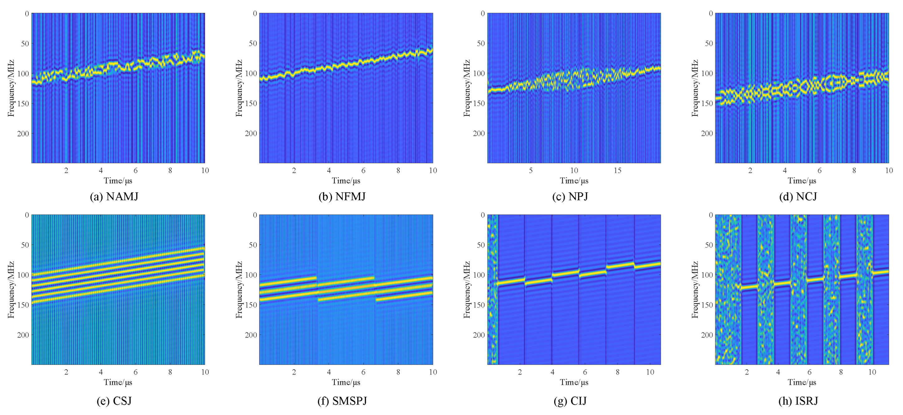
In this paper, we employ the Choi-Williams distribution (CWD) to perform time-frequency analysis on radar jamming signals. The CWD is a bilinear time-frequency transform known for its ability to provide high-resolution representations of non-stationary signals in the joint time-frequency domain. It is important to note that the CWD is particularly effective at reducing cross-terms and enhancing concentration in the time-frequency plane, making it a valuable tool for analyzing non-stationary signals, including radar jamming signals. However, it should be acknowledged that the CWD may have limitations in cases where signals contain components that share similar time and frequency characteristics, as it may not be as effective in distinguishing such components. Nevertheless, for the time-varying spectral analysis of radar jamming signals, the CWD is a well-suited choice. By applying the CWD, we can effectively analyze the jamming present in the radar returns and develop algorithms for jamming identification. Figure 2 shows the CWD time-frequency representation of the 8 types of radar jamming signals in Section 2.

The CWD belongs to the Cohen class of time-frequency distributions, which are bilinear transforms that reveal the joint time-frequency content of nonstationary signals. The general Cohen class is defined by:

$$C_x(t,\omega )=\int \int x(u+\frac{\tau }{2})x^{*}(u-\frac{\tau }{2})\psi (t-u,\tau )e^{-j\omega \tau }dud\tau$$

(13)

where $\psi (t-u,\tau )$ is the time-frequency kernel function.

By setting $\psi (t-u,\tau )=\sqrt{\frac{\sigma }{4\pi {\tau }^2}}exp(-\frac{\sigma {(t-u)}^2}{4{\tau }^2})$, CWD is obtained as follows:

$$\begin{array}{c}\hfill CW{D}_x\left(t,f\right)=\int \int \sqrt{\frac{\sigma }{4\pi {\tau }^2}}{e}^{-\frac{\sigma {(t-u)}^2}{4{\tau }^2}}x\left(u+\frac{\tau }{2}\right)\\ \hfill x^{*}\left(u-\frac{\tau }{2}\right){\mathrm{e}}^{-\mathrm{j}2\pi ft}dud\tau \end{array}$$

(14)

where $CW{D}_x\left(t,f\right)$ represents the Choi-Williams distribution of signal x(t) at time t and frequency f, $\sigma$ controls the width of the kernel function, u and $\tau$ are integration variables.

3.2. Diagram Denoising with Diffusion Model

Raw time-frequency diagrams exhibit noise and clutter that can obscure the useful signal components. Here we leverage diffusion models based on a U-Net architecture to filter out noise and recover cleaner time-frequency representations.

In the forward process, we gradually add Gaussian noise to the input noisy time-frequency map $x_0$ in T timesteps as follows:

$$q\left(x_{t+1}\right|x_t)=\mathcal{N}(x_{t+1};\sqrt{1-{\beta }_t}{x}_t,{\beta }_t\mathbf{I})$$

(15)

where ${\beta }_t$ is the noise schedule that controls the variance of the added Gaussian noise at timestep t, $\mathbf{I}$ is the identity matrix.

By performing T iterations of adding small Gaussian noise, we obtain a highly noisy time-frequency map $x_T$:

$$x_T=x_0+ϵ,ϵ\sim \mathcal{N}(0,\Sigma )$$

(16)

where $\Sigma$ is the accumulated noise covariance. This forward process injects noises at different scales into the input and destroys its original structure.

The forward process acts as a form of regularization that smooths the noise-conditional distribution $q\left(x_t\right|x_0)$ for better generation. It is a key component that enables the diffusion model to remove noise and recover clean signals in the reverse process.

In the reverse process, we aim to recover the clean time-frequency map $x_0$ from the noisy inputs $x_0,x_1,\dots ,x_T$ in a recursive manner. A conditional diffusion model with a U-Net decoder is used to perform iterative denoising.

The U-Net decoder takes $x_t$ and extracted feature representations $h_t$ as input, and predicts the noise residual ${ϵ}_{\theta }(x_t,t)$ for denoising:

$${ϵ}_{\theta }(x_t,t)=\sqrt{1-{\overline{\alpha }}_t}(x_t-\sqrt{\overline{\alpha }t}{x}_{t-1})$$

(17)

where ${\overline{\alpha }}_t$ is the denoising strength and $\theta$ denotes decoder parameters.

The denoised signal ${\widehat{x}}_{t-1}$ can be obtained by removing the predicted noise residual:

$$\begin{array}{cc}\hfill {\widehat{x}}_{t-1}& \hfill =\frac{1}{\sqrt{1-\overline{\alpha }t}}(x_t-{ϵ}_{\theta }(x_t,t))\hfill \\ \hfill & \hfill =\sqrt{\overline{\alpha }t}{x}_{t-1}+(1-\sqrt{{\overline{\alpha }}_t})x_t\hfill \end{array}$$

(18)

By starting from $x_T$ and performing T denoising iterations, we can recover the clean time-frequency map ${\widehat{x}}_0$. The U-Net leverages multiscale features and temporal conditioning to enable effective signal denoising.

3.3. Multi-Scale Feature Extraction Using Swin Transformer

Robust feature extraction is key to distinguishing different types of jamming signals. In this section, we utilize SwinT to extract discriminative time-frequency features from denoised CWD diagrams $\mathbf{X}\in {\mathbb{R}}^{H\times W\times C}$ for radar jamming signal classification.

3.3.1. Patch Embedding

In SwinT, patch embedding is performed as a preprocessing step to convert an input image into a sequence of token embeddings. Specifically, given an input image $\mathbf{X}\in {\mathbb{R}}^{H\times W\times C}$, it is divided into non-overlapping patches of size $P\times P$:

$$x_p=\mathbf{X}[p_h:p_h+P,p_w:p_w+P,:]\in {\mathbb{R}}^{P\times P\times C}$$

(19)

where $p=(p_h,p_w)$ denotes the top-left coordinate of the patch. Each patch $x_p$ is then flattened and projected to a D-dimensional vector through a linear projection layer:

$${\mathbf{z}}_p^0=\mathrm{Linear}\left(x_p\right)\in {\mathbb{R}}^D$$

(20)

In addition, a learnable 1D position encoding is added to retain spatial information:

$${\mathbf{z}}_p=[{\mathbf{z}}_p^0;{\mathbf{e}}_p]\in {\mathbb{R}}^{D+1}$$

(21)

where ${\mathbf{e}}_p$ denotes the position encoding for patch p. The sequence of patch embeddings $\left\{{\mathbf{z}}_p\right\}$ are then input to the subsequent Transformer encoder layers.

According to the above process, we partition the CWD of each radar jamming signal into non-overlapping patches of size 4 × 4, and obtain patch embeddings. These patch tokens capture local time-frequency information. We then feed the patch sequence into the hierarchical modules of SwinT. The network can learn time-frequency characteristics at different scales, and integrate multi-scale information for powerful graph representation, thereby achieving effective identification of radar jamming signals.

3.3.2. Patch Merging

Patch merging is performed to reduce the sequence length and computation cost. After processing through several Transformer encoder layers with patch embeddings of size $P\times P$, patch merging aggregates neighboring patches into a larger patch to downsample the spatial dimensions.

Specifically, the input sequence of patch tokens $\mathbf{z}\in {\mathbb{R}}^{N\times (D+1)}$ is first reshaped to $\mathbf{z}\in {\mathbb{R}}^{H/P\times W/P\times (D+1)}$. For each non-overlapping 2 × 2 patch block ${\mathbf{z}}_b\in {\mathbb{R}}^{2\times 2\times (D+1)}$, patch merging is applied by first averaging the positional encodings ${\mathbf{e}}_b$ of the 4 patches, then concatenating and linearly projecting the patch embeddings to a lower dimension:

$$\begin{array}{cc}\hfill {\overline{\mathbf{e}}}_b& \hfill =\mathrm{Average}\left({\mathbf{e}}_b\right)\hfill \end{array}$$

(22)

$$\begin{array}{cc}\hfill {\widehat{\mathbf{z}}}_b& \hfill =\mathrm{Linear}\left(\mathrm{Concat}\left({\mathbf{z}}_b^0\right)\right)\hfill \end{array}$$

(23)

The merged patch token is then constructed by concatenating ${\widehat{\mathbf{z}}}_b$ and ${\overline{\mathbf{e}}}_b$. This reduces the number of patches by a factor of 4. The new sequence of downsampled patch tokens is then input to subsequent Transformer encoder layers, which adopt larger patch sizes.

Through such hierarchical patch merging, SwinT can efficiently process the input time-frequency representations of radar jamming signals. This architecture also allows the network to integrate fine-grained and coarse-grained features to learn representations.

3.3.3. Shifted Window Attention

The standard self-attention in Transformers relates all tokens in the sequence to each other, which leads to a quadratic computational complexity. To improve efficiency, SwinT adopts a shifted window-based self-attention, where each token only attends to tokens within a local window.

Formally, given an input feature map $\mathbf{X}\in {\mathbb{R}}^{H\times W\times C}$, it is first partitioned into non-overlapping windows of size $M\times M$:

$${\mathbf{X}}_{i,j}=\mathbf{X}[iM:(i+1)M,jM:(j+1)M,:]$$

(24)

where $(i,j)$ indexes the windows. The self-attention is then performed within each window ${\mathbf{X}}_{i,j}$ independently.

To enable communication between windows, SwinT shifts the window partitioning in consecutive self-attention layers. For example, in the next layer, the windows are shifted by $M/2$:

$${\mathbf{X}}_{i,j}^{\prime }=\mathbf{X}[iM+\frac{M}{2}:(i+1)M+\frac{M}{2},jM+\frac{M}{2}:(j+1)M+\frac{M}{2},:]$$

(25)

Therefore, each token can attend to different tokens from overlapping windows in different layers. This achieves a balance between efficiency and modeling power.

The shifted window attention restricts self-attention to local regions while allowing global communication across layers. It enables SwinT to model both local and global dependencies in an efficient manner.

3.3.4. Transformer Block

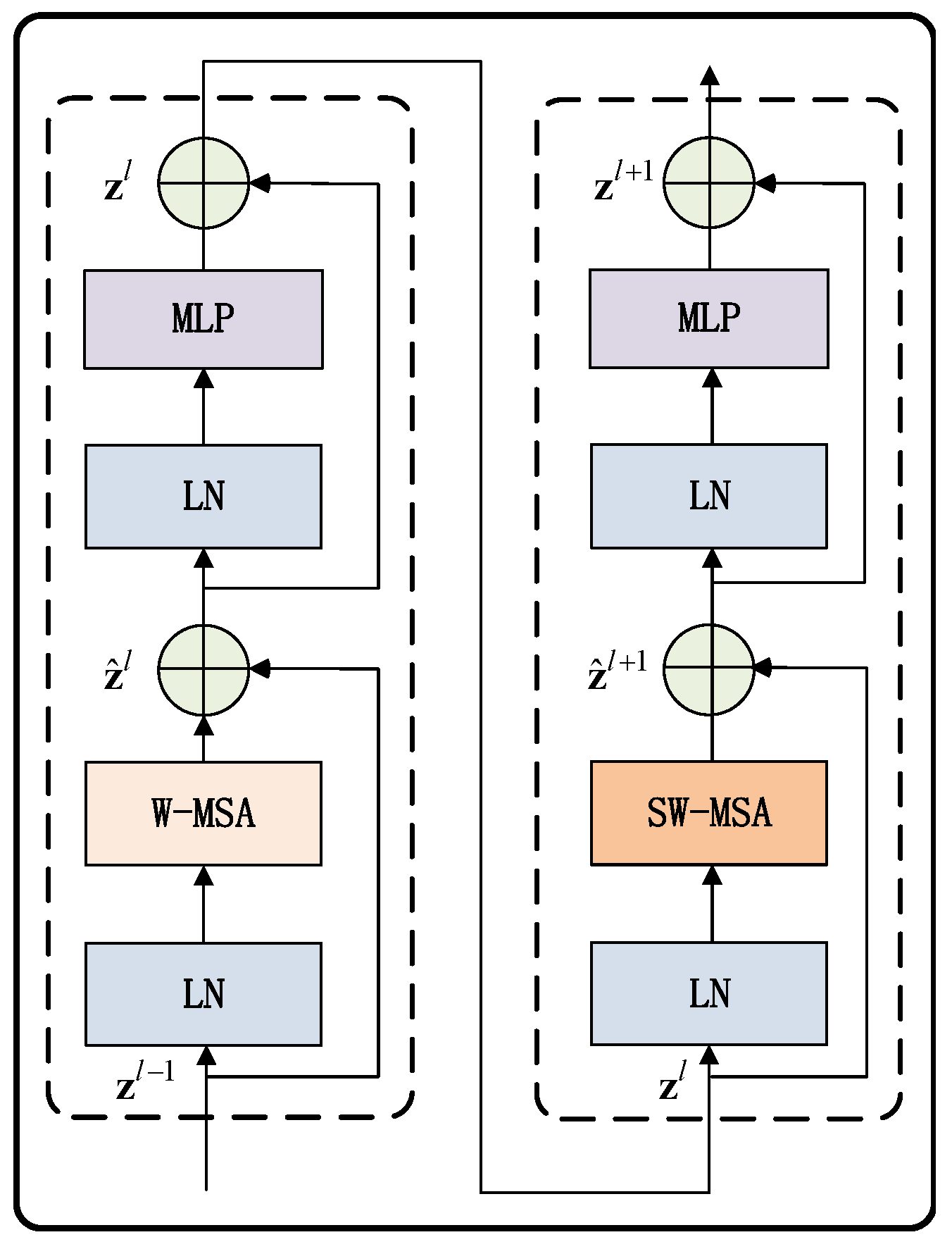
The basic building block of the SwinT is the Transformer Block (Figure 3). Each block contains two types of Multi-Head Self-Attention (MSA) layers: a Window-based MSA (W-MSA) and a Shifted Window MSA (SW-MSA).

Specifically, given an input feature map $z^l\in {\mathbb{R}}^{H\times W\times C}$, it first goes through a LayerNorm (LN) and then a W-MSA layer, where attention is computed within local windows. This is followed by another LN and a Multilayer Perceptron (MLP) for feedforward processing.

The output feature map is then fed to a SW-MSA, which shifts the window partitioning. This block design allows modeling both local and global dependencies. The input feature map is added back after each MSA and MLP sub-layer:

$$\begin{array}{cc}\hfill z^{\prime l}& \hfill =z^l+\mathrm{W}\text{-}\mathrm{MSA}\left(LN\left(z^l\right)\right)\hfill \end{array}$$

(26)

$$\begin{array}{cc}\hfill z^{″l}& \hfill =z^{\prime l}+\mathrm{MLP}\left(LN\left(z^{\prime l}\right)\right)\hfill \end{array}$$

(27)

$$\begin{array}{cc}\hfill z^{l+1}& \hfill =z^{″l}+\mathrm{SW}\text{-}\mathrm{MSA}\left(LN\left(z^{″l}\right)\right)\hfill \end{array}$$

(28)

A residual connection and LayerNorm are applied after each sub-layer to facilitate training and improve performance. The SwinT Block integrates window-based self-attention and shifted window design, which are key innovations of SwinT, enabling efficient modeling of both local and global contextual information for visual recognition tasks.

3.4. Classification with a Linear Prediction Head

For accurate classification, the extracted features are projected into label space using a prediction head composed of linear layers before softmax output.

Given an input feature map x from Swin Transformer with shape [B, L, C], layer normalization is first applied to normalize the features:

$$\widehat{\mathbf{x}}=\mathrm{LayerNorm}\left(x\right)$$

(29)

Then global average pooling is performed across the spatial dimensions to aggregate spatial information. The input is transposed to [B, C, L] and average pooled on L, outputting a feature map y with shape [B, C, 1]:

$$y=\mathrm{AvgPool}\left({\widehat{\mathbf{x}}}^T\right)\in {\mathbb{R}}^{B\times C\times 1}$$

(30)

Next, flatten is applied to squeeze y to [B, C]:

$$z=\mathrm{Flatten}\left(y\right)\in {\mathbb{R}}^{B\times C}$$

(31)

Finally, a fully-connected layer is used to map z to classification outputs $\widehat{y}$:

$$\widehat{y}=\mathrm{Linear}\left(z\right)$$

(32)

This module applies normalization, spatial aggregation through pooling, flattening and a linear classifier on top of Swin Transformer features to effectively perform image classification with simplified computations.

3.5. Loss Function Design

The training process of the proposed model consists of two stage tasks: image denoising based on diffusion model and image recognition using Swin Transformer. The overall loss function is designed as a weighted sum of the individual loss terms for each task:

$${\mathcal{L}}_{\mathrm{t}}={\lambda }_{\mathrm{d}}{\mathcal{L}}_{\mathrm{d}}+{\lambda }_{\mathrm{c}}{\mathcal{L}}_{\mathrm{c}}$$

(33)

where ${\lambda }_{\mathrm{d}}$ and ${\lambda }_{\mathrm{c}}$ are the weights to balance between the two losses.

For the time-frequency distribution denoising task, in order to obtain a reverse diffusion model that can restore the corrupted time-frequency distributions back to clean distributions, during training we use images without added noise as input, and use the mean squared error (MSE) between the input image x and output image $x^{\prime }$ as the loss term:

$${\mathcal{L}}_{\mathrm{d}}=\mathrm{MSE}(x,x^{\prime })=\frac{1}{n}\sum _{i=1}^n{(x_i-x_i^{\prime })}^2$$

(34)

The image recognition task is formulated as a classification problem. The cross-entropy loss between the predicted class probabilities y and ground-truth labels t is used:

$${\mathcal{L}}_{\mathrm{c}}=\mathrm{CrossEntropyLoss}(y,t)=-\sum _{c=1}^C{t}_{c}log\left(y_c\right)$$

(35)

where C is the number of classes.

By optimizing this weighted multi-task loss, the model can be trained to balance the denoising reconstruction and recognition accuracy. The loss weights $\lambda$ allow adjusting the difficulty of training each component.

4. Experiments

4.1. Experimental Settings

The dataset contains 8 types of jamming signals, including NAMJ, NFMJ, NCJ, NPJ, CSJ, SMSPJ, CIJ and ISRJ. Based on the mathematical models in Section 2 and the CWD generation method in Section 3.1, the corresponding time-frequency distributions are generated for each jamming type to construct the image dataset.

The JNR levels are set from $-16\mathrm{dB}$ to $6\mathrm{dB}$ with $2\mathrm{dB}$ spacing. For each jamming category, 100 samples are generated under each JNR, totaling 9600 samples. 45% of the data set is used as the training set, 15% is used as the validation set, and 30% as the test set.

Table 1. Parameterization of Radar Jamming signals.

Jamming Type	Parameter	Range
NAMJ	Amplitude	5–10
	Frequency	100–150 MHz
	bandwidth	10–30 MHz
NFMJ	Amplitude	5–10
	Frequency	100–150 MHz
	bandwidth	10–30 MHz
	effective modulation index	0.5–0.75
NCJ	Amplitude	5–10
	Frequency	100–150 MHz
	bandwidth	10–30 MHz
NPJ	Amplitude	5–10
	Frequency	100–150 MHz
	bandwidth	10–30 MHz
CSJ	Amplitude	5–10
	Frequency	100–150 MHz
	bandwidth	10–30 MHz
	Comb teeth number	4–8
SMSPJ	Amplitude	5–10
	Frequency	100–150 MHz
	bandwidth	10–30 MHz
	Sampling Multiple	2–4
CIJ	Amplitude	5–10
	Frequency	100–150 MHz
	bandwidth	2–10 MHz
	Sub-pulse Number	2–10
	Retransmission Number	4–8
ISRJ	Amplitude	5–10
	Frequency	100–150 MHz
	bandwidth	2–10 MHz
	sampling number	3–5

summarizes the parameter settings for different jamming types. During training and validation, data covering the −16 dB to 6 dB JNR range were used together. For testing, evaluations were done at each specific JNR level using the corresponding test set for that level.

In the upcoming experiments, the parameters are set as follows: the dataset images are uniformly resized to 224 × 224, the optimization process utilizes the Adam optimizer with a learning rate of 0.0001 and a weight decay of 0.05, the batch size is 20, the time steps T for the diffusion model is 1000, and the window size M in the Swin Transformer is set as 7.

4.2. Results & Analysis

4.2.1. Recognition Performance of Swin-Transformer

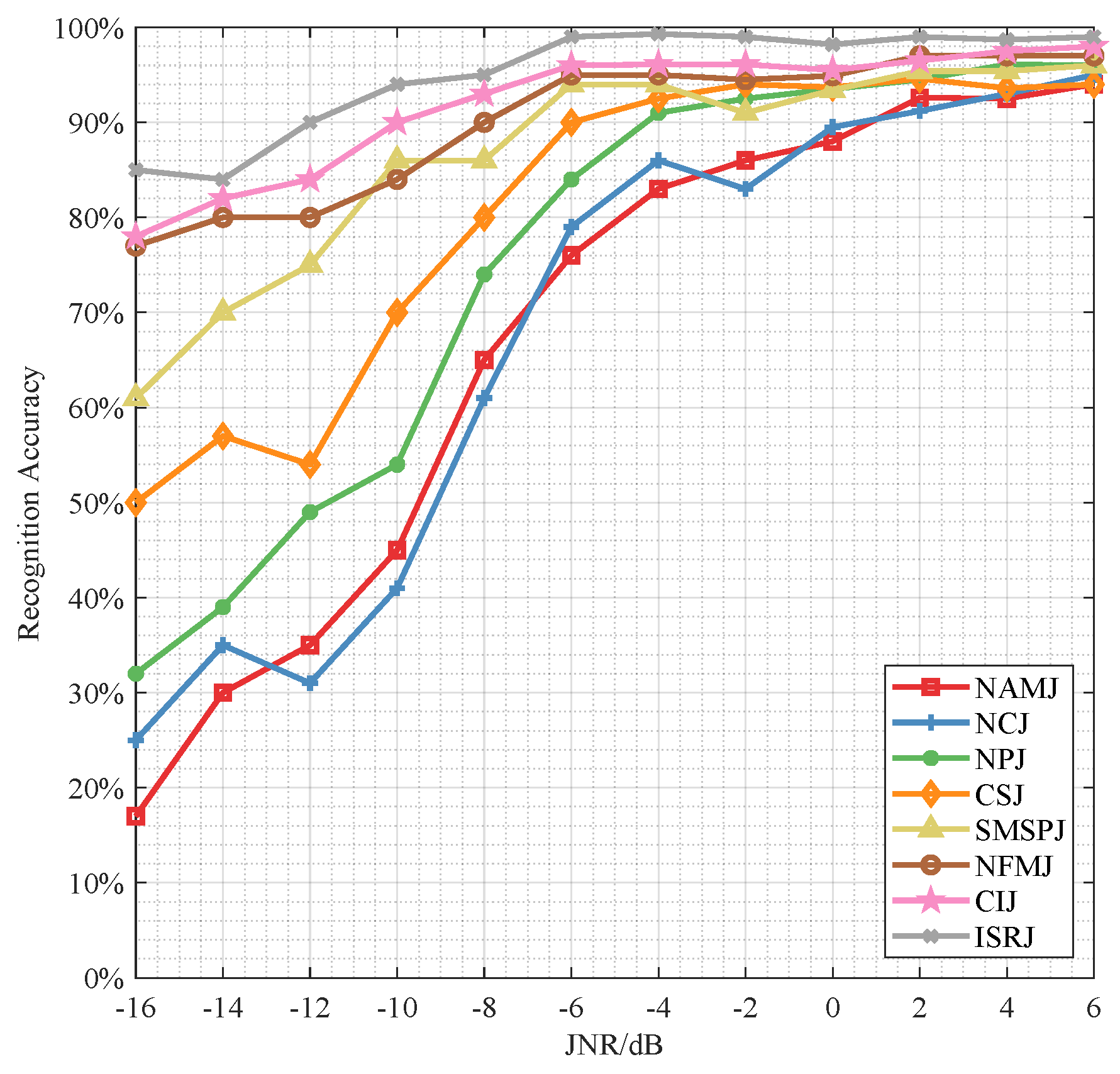
In the first experiment, we evaluate the recognition performance of Swin Transformer on 8 different radar jamming types. From Figure 4, it can be seen that Swin Transformer only shows certain robustness for some of the tested radar jamming. At extremely low JNR between −16 dB and −10 dB, the identification accuracy for ISRJ, CIJ, NFMJ can be maintained between 76% to 95%, while NAMJ, NCJ, NPJ gradually increase from 17–32% to 45–54%. At −4 dB, the recognition accuracy for all jamming types reaches above 80%, and exceeds 90% for all jammings at 2 dB as JNR increases.

4.2.2. Recognition Performance of Diff-Swin-Transformer

In this part, we evaluate the recognition performance of our proposed Diff-SwinT algorithm.

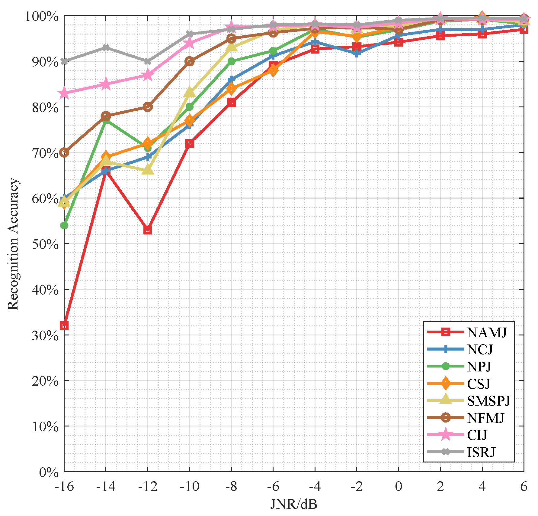
The recognition accuracy under different jamming types and JNR levels is shown in Figure 5. It can be observed that compared to the first experiment without using the diffusion-based denoising module, the proposed algorithm demonstrates stronger robustness for all the tested jamming. At low JNR of −16 dB, the identification accuracy is improved by 22%, 9%, 35%, 15% for NPJ, CSJ, NCJ, NAMJ respectively. As JNR increases to −10 dB, the improvement becomes 26%, 7%, 35%, 27% for these four jamming types. Overall, the recognition rate for all jamming types exceeds 70% at JNR = −10 dB, exceeds 80% at JNR = −8 dB, exceeds 90% at JNR = −4 dB, and gradually increases to around 95% as JNR rises.

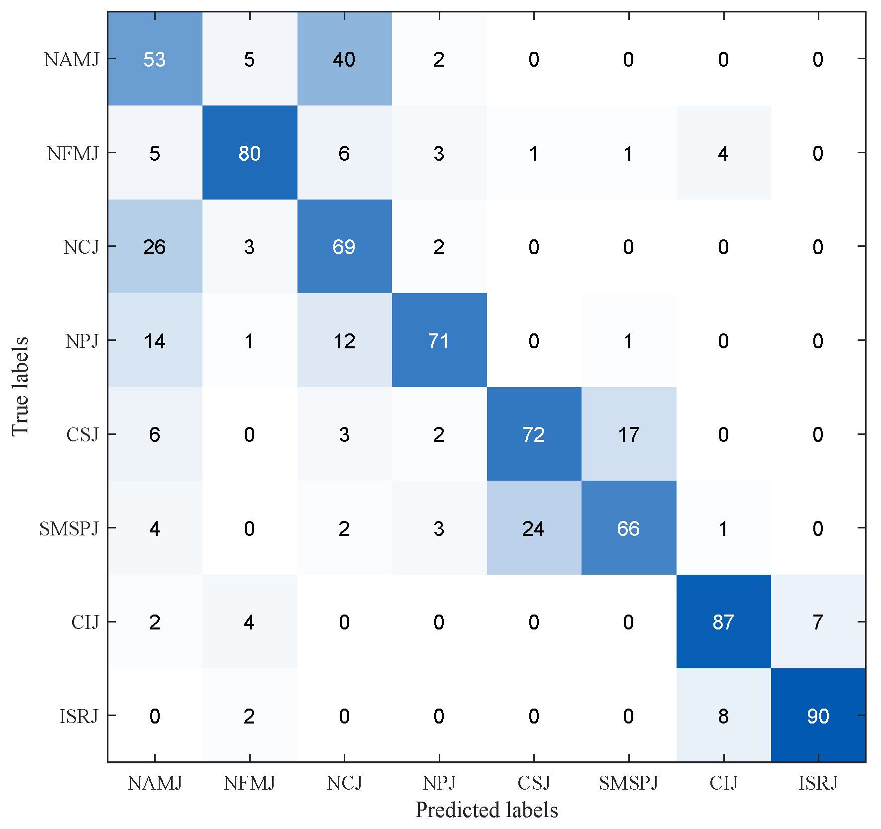
Additionally, we show the confusion matrix obtained using the proposed algorithm at JNR = −12 dB in Figure 6, where the vertical axis is the true label and the horizontal axis is the predicted label. It can be observed that under low SNR, NAMJ and NCJ, two radar jamming types with very different generation mechanisms, are highly confused. This is because their time-frequency representations look similar under comparable modulation bandwidth and chirp rate, as can be seen from Figure 2. The same situation occurs between CSJ and NCJ as well.

4.2.3. Comparison with Other Methods

In this part, we evaluate the recognition accuracy and the computational complexity of four algorithms: Diff-SwinT, Swin-Transformer, VGG-Net (Visual Geometry Group Network) [22], and FFB (Feature Fusion Based) [46] under different JNR levels from −16 dB to 6 dB.

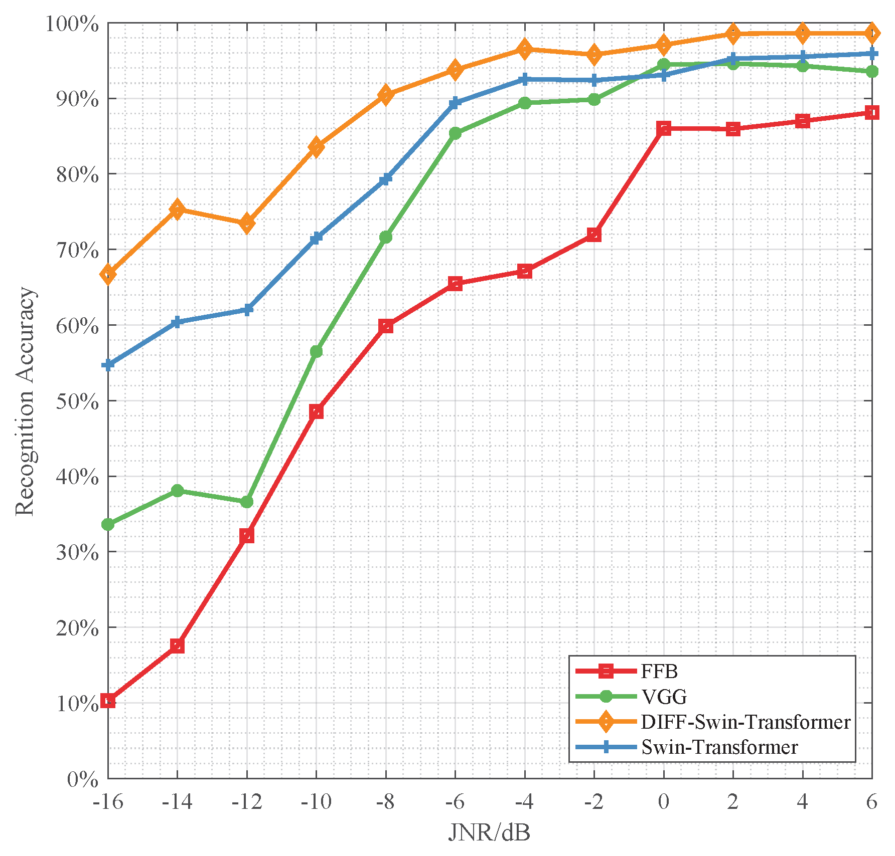
From Figure 7, we can see that our proposed Diff-SwinT achieves superior performance over VGG and FFB at all JNR levels. Specifically, at extremely low JNRs between −16 dB and −10 dB, Diff-SwinT obtains 66.7–83.5% accuracy, outperforming VGG and FFB by 56.7–27%, with the advantage expanding as JNR decreases. As JNR increases from −10 dB to 6 dB, the performance gap gradually reduces but remains significant, with the overall recognition rate of Diff-SwinT reaching 90% at JNR = −8 dB, and gradually increasing to 98.6%. VGG and FFB reach above 80% at JNR = −6 dB and 0 dB respectively, and continue to increase to around 94% and 88%.

Table 2. The Computational Cost of Four Methods.

Method	Parameters (M)	FLOPs (G)	Time (ms)
VGG	138.36	15.50	15.42
FFB	-	-	7.01
SwinT	28.29	4.36	8.22
DIFF-SwinT	59.41	10.52	12.54

shows the number of learnable parameters, floating point operations (FLOPs), and per-sample inference time on the hardware platform (Intel i7-12700H CPU and NVIDIA GeForce RTX 3060 with 6GB) for the four methods. It can be seen that although Diff-SwinT has more parameters and FLOPs than SwinT, it still has fewer parameters and FLOPs than VGG. Moreover, Diff-SwinT achieves slightly faster inference time compared to VGG.

While SwinT alone outperforms prior methods, its recognition accuracy still degraded significantly under low JNRs. Owing to the diffusion-based denoising module, compared to using Swin Transformer alone, Diff-SwinT achieves around 10% identification rate improvement at JNR between −16 dB and −8 dB. This ablation experiment clearly verifies the efficacy of the denoising module in enhancing model robustness under strong noise environments.

5. Conclusions

For radar jamming recognition, this paper proposed Diff-SwinT, a novel integrated framework that identified various typical radar jamming more accurately under low JNR conditions. This method fully utilized denoising techniques based on the diffusion model to bolster robustness and capitalized on the strength of SwinT in extracting multi-scale features from radar time-frequency representations. Simulation results demonstrated that the Diff-SwinT algorithm achieved remarkable overall accuracy up to 83.5% at JNR = −10 dB and over 95% at −4 dB. When compared to using Swin Transformer alone, Diff-SwinT significantly improved overall accuracy by 15% to 11% from JNR −16 dB to −10 dB. In comparison to VGG-based and feature fusion-based recognition methods, Diff-SwinT showed substantially higher overall accuracy of 33% to 27% and 57% to 35%, respectively, from JNR −16 dB to −10 dB. This verified the efficacy of the proposed integrated framework and its considerable advantages over existing algorithms. In summary, the proposed Diff-SwinT framework provided a new paradigm for robust radar jamming recognition under challenging low JNR conditions.

References

- Neng-Jing, L.; Yi-Ting, Z. A survey of radar ECM and ECCM. IEEE Trans. Aerosp. Electron. Syst. 1995, 31, 1110–1120. [Google Scholar] [CrossRef]
- Xiao, L.; Yang, P.; Lei, X.; Xiao, Y.; Fan, S.; Li, S.; Xiang, W. A Low-Complexity Detection Scheme for Differential Spatial Modulation. IEEE Commun. Lett. 2015, 19, 1516–1519. [Google Scholar] [CrossRef]
- Qu, Q.; Wei, S.; Liu, S.; Liang, J.; Shi, J. JRNet: Jamming recognition networks for radar compound suppression jamming signals. IEEE Trans. Veh. Technol. 2020, 69, 15035–15045. [Google Scholar] [CrossRef]
- Yao, Z.; Fu, X.; Guo, L.; Wang, Y.; Lin, Y.; Shi, S.; Gui, G. Few-Shot Specific Emitter Identification Using Asymmetric Masked Auto-Encoder. IEEE Commun. Lett. 2023, 27, 2657–2661. [Google Scholar] [CrossRef]
- Hou, L.; Zhang, S.; Wang, C.; Li, X.; Chen, S.; Zhu, L.; Zhu, Y. Jamming Recognition of Carrier-Free UWB Cognitive Radar Based on MANet. IEEE Trans. Instrum. Meas. 2023, 72, 1–13. [Google Scholar] [CrossRef]
- Zha, H.; Wang, H.; Feng, Z.; Xiang, Z.; Yan, W.; He, Y.; Lin, Y. LT-SEI: Long-Tailed Specific Emitter Identification Based on Decoupled Representation Learning in Low-Resource Scenarios. IEEE Trans. Intell. Transp. Syst. 2023, 1–15. [Google Scholar] [CrossRef]
- Zhou, F.; Zhao, B.; Tao, M.; Bai, X.; Chen, B.; Sun, G. A Large Scene Deceptive Jamming Method for Space-Borne SAR. IEEE Trans. Geosci. Remote Sens. 2013, 51, 4486–4495. [Google Scholar] [CrossRef]
- Lan, L.; Xu, J.; Liao, G.; Zhang, Y.; Fioranelli, F.; So, H.C. Suppression of Mainbeam Deceptive Jammer With FDA-MIMO Radar. IEEE Trans. Veh. Technol. 2020, 69, 11584–11598. [Google Scholar] [CrossRef]
- Ma, Z.; Xiang, W.; Long, H.; Wang, W. Proportional Fair Resource Partition for LTE-Advanced Networks with Type I Relay Nodes. In Proceedings of the 2011 IEEE International Conference on Communications (ICC), Kyoto, Japan, 5–9 June 2011; pp. 1–5. [Google Scholar] [CrossRef]
- Su, D.; Gao, M. Research on Jamming Recognition Technology Based on Characteristic Parameters. In Proceedings of the 2020 IEEE 5th International Conference on Signal and Image Processing (ICSIP), Nanjing, China, 3–5 July 2020; pp. 303–307. [Google Scholar] [CrossRef]
- Qu, Q.; Wang, Y.L.; Liu, W.; Wei, S.; Du, Q. IRNet: Interference Recognition Networks for Automotive Radars via Autocorrelation Features. IEEE Trans. Microw. Theory Tech. 2022, 70, 2762–2774. [Google Scholar] [CrossRef]
- Wang, Q.; Du, P.; Yang, J.; Wang, G.; Lei, J.; Hou, C. Transferred deep learning based waveform recognition for cognitive passive radar. Signal Process. 2019, 155, 259–267. [Google Scholar] [CrossRef]
- Hou, C.; Liu, G.; Tian, Q.; Zhou, Z.; Hua, L.; Lin, Y. Multisignal Modulation Classification Using Sliding Window Detection and Complex Convolutional Network in Frequency Domain. IEEE Internet Things J. 2022, 9, 19438–19449. [Google Scholar] [CrossRef]
- Feng, Z.; Zha, H.; Xu, C.; He, Y.; Lin, Y. FCGCN: Feature Correlation Graph Convolution Network for Few-Shot Individual Identification. IEEE Trans. Consum. Electron. 2023, 1. [Google Scholar] [CrossRef]
- Lv, Q.; Quan, Y.; Feng, W.; Sha, M.; Dong, S.; Xing, M. Radar Deception Jamming Recognition Based on Weighted Ensemble CNN With Transfer Learning. IEEE Trans. Geosci. Remote Sens. 2022, 60, 1–11. [Google Scholar] [CrossRef]
- Wei, S.; Qu, Q.; Zeng, X.; Liang, J.; Shi, J.; Zhang, X. Self-Attention Bi-LSTM Networks for Radar Signal Modulation Recognition. IEEE Trans. Microw. Theory Tech. 2021, 69, 5160–5172. [Google Scholar] [CrossRef]
- Dong, G.; Liu, H. Signal Augmentations Oriented to Modulation Recognition in the Realistic Scenarios. IEEE Trans. Commun. 2023, 71, 1665–1677. [Google Scholar] [CrossRef]
- Bao, Z.; Lin, Y.; Zhang, S.; Li, Z.; Mao, S. Threat of Adversarial Attacks on DL-Based IoT Device Identification. IEEE Internet Things J. 2022, 9, 9012–9024. [Google Scholar] [CrossRef]
- Liu, M.; Liu, Z.; Lu, W.; Chen, Y.; Gao, X.; Zhao, N. Distributed Few-Shot Learning for Intelligent Recognition of Communication Jamming. IEEE J. Sel. Top. Signal Process. 2022, 16, 395–405. [Google Scholar] [CrossRef]
- Luo, Z.; Cao, Y.; Yeo, T.S.; Wang, Y.; Wang, F. Few-Shot Radar Jamming Recognition Network via Time-Frequency Self-Attention and Global Knowledge Distillation. IEEE Trans. Geosci. Remote Sens. 2023, 61, 1–12. [Google Scholar] [CrossRef]
- Lin, Y.; Tu, Y.; Dou, Z. An Improved Neural Network Pruning Technology for Automatic Modulation Classification in Edge Devices. IEEE Trans. Veh. Technol. 2020, 69, 5703–5706. [Google Scholar] [CrossRef]
- Zhou, H.; Wang, L.; Ma, M.; Guo, Z. Compound radar jamming recognition based on signal source separation. Signal Process. 2024, 214, 109246. [Google Scholar] [CrossRef]
- Zhang, Z.; Li, Y.; Zhai, Q.; Li, Y.; Gao, M. Mode Recognition of Multifunction Radars for Few-Shot Learning Based on Compound Alignments. IEEE Trans. Aerosp. Electron. Syst. 2022, 58, 5860–5874. [Google Scholar] [CrossRef]
- Long, H.; Xiang, W.; Wang, J.; Zhang, Y.; Wang, W. Cooperative jamming and power allocation with untrusty two-way relay nodes. IET Commun. 2014, 8, 2290–2297. [Google Scholar] [CrossRef]
- Lin, Y.; Zha, H.; Tu, Y.; Zhang, S.; Yan, W.; Xu, C. GLR-SEI: Green and Low Resource Specific Emitter Identification Based on Complex Networks and Fisher Pruning. IEEE Trans. Emerg. Top. Comput. Intell. 2023, 1–12. [Google Scholar] [CrossRef]
- Ya, T.; Yun, L.; Haoran, Z.; Zhang, J.; Yu, W.; Guan, G.; Shiwen, M. Large-scale real-world radio signal recognition with deep learning. Chin. J. Aeronaut. 2022, 35, 35–48. [Google Scholar] [CrossRef]
- Zhu, M.; Li, Y.; Pan, Z.; Yang, J. Automatic modulation recognition of compound signals using a deep multi-label classifier: A case study with radar jamming signals. Signal Process. 2020, 169, 107393. [Google Scholar] [CrossRef]
- Ravi Kishore, T.; Rao, K.D. Automatic Intrapulse Modulation Classification of Advanced LPI Radar Waveforms. IEEE Trans. Aerosp. Electron. Syst. 2017, 53, 901–914. [Google Scholar] [CrossRef]
- Hoang, L.M.; Kim, M.; Kong, S.H. Automatic Recognition of General LPI Radar Waveform Using SSD and Supplementary Classifier. IEEE Trans. Signal Process. 2019, 67, 3516–3530. [Google Scholar] [CrossRef]
- Lin, Y.; Zhao, H.; Ma, X.; Tu, Y.; Wang, M. Adversarial Attacks in Modulation Recognition With Convolutional Neural Networks. IEEE Trans. Reliab. 2021, 70, 389–401. [Google Scholar] [CrossRef]
- Huynh-The, T.; Doan, V.S.; Hua, C.H.; Pham, Q.V.; Nguyen, T.V.; Kim, D.S. Accurate LPI Radar Waveform Recognition With CWD-TFA for Deep Convolutional Network. IEEE Wirel. Commun. Lett. 2021, 10, 1638–1642. [Google Scholar] [CrossRef]
- Zhu, M.; Li, Y.; Wang, S. Model-Based Time Series Clustering and Interpulse Modulation Parameter Estimation of Multifunction Radar Pulse Sequences. IEEE Trans. Aerosp. Electron. Syst. 2021, 57, 3673–3690. [Google Scholar] [CrossRef]
- Lin, Y.; Tu, Y.; Dou, Z.; Chen, L.; Mao, S. Contour Stella Image and Deep Learning for Signal Recognition in the Physical Layer. IEEE Trans. Cogn. Commun. Netw. 2021, 7, 34–46. [Google Scholar] [CrossRef]
- Chao, Z.; Quanhua, L.; Cheng, H. Time-frequency analysis techniques for recognition and suppression of interrupted sampling repeater jamming. J. Radars 2019, 8, 100–106. [Google Scholar] [CrossRef]
- Zhang, J.; Liang, Z.; Zhou, C.; Liu, Q.; Long, T. Radar Compound Jamming Cognition Based on a Deep Object Detection Network. IEEE Trans. Aerosp. Electron. Syst. 2023, 59, 3251–3263. [Google Scholar] [CrossRef]
- Zhang, Y.; Wei, Y.; Yu, L. Interrupted sampling repeater jamming recognition and suppression based on phase-coded signal processing. Signal Process. 2022, 198, 108596. [Google Scholar] [CrossRef]
- Croitoru, F.A.; Hondru, V.; Ionescu, R.T.; Shah, M. Diffusion Models in Vision: A Survey. IEEE Trans. Pattern Anal. Mach. Intell. 2023, 45, 10850–10869. [Google Scholar] [CrossRef]
- Özbey, M.; Dalmaz, O.; Dar, S.U.; Bedel, H.A.; Özturk, Ş.; Güngör, A.; Çukur, T. Unsupervised Medical Image Translation with Adversarial Diffusion Models. IEEE Trans. Med. Imaging 2023, 1. [Google Scholar] [CrossRef]
- Liu, C.; Fu, X.; Wang, Y.; Guo, L.; Liu, Y.; Lin, Y.; Zhao, H.; Gui, G. Overcoming data limitations: A few-shot specific emitter identification method using self-supervised learning and adversarial augmentation. IEEE Trans. Inf. Forensics Secur. 2023; early access. [Google Scholar] [CrossRef]
- Han, K.; Wang, Y.; Chen, H.; Chen, X.; Guo, J.; Liu, Z.; Tang, Y.; Xiao, A.; Xu, C.; Xu, Y.; et al. A Survey on Vision Transformer. IEEE Trans. Pattern Anal. Mach. Intell. 2023, 45, 87–110. [Google Scholar] [CrossRef]
- Liu, Z.; Lin, Y.; Cao, Y.; Hu, H.; Wei, Y.; Zhang, Z.; Lin, S.; Guo, B. Swin Transformer: Hierarchical Vision Transformer using Shifted Windows. In Proceedings of the 2021 IEEE/CVF International Conference on Computer Vision (ICCV), Montreal, BC, Canada, 11–17 October 2021; pp. 9992–10002. [Google Scholar] [CrossRef]
- Lin, A.; Chen, B.; Xu, J.; Zhang, Z.; Lu, G.; Zhang, D. DS-TransUNet: Dual Swin Transformer U-Net for Medical Image Segmentation. IEEE Trans. Instrum. Meas. 2022, 71, 1–15. [Google Scholar] [CrossRef]
- Minhong, S.; Bin, T. Noise amplitude modulation jamming signal suppression based on weighted-matching pursuit. J. Syst. Eng. Electron. 2009, 20, 962–967. [Google Scholar]
- Hao, H.; Zeng, D.; Ge, P. Research on the Method of Smart Noise Jamming on Pulse Radar. In Proceedings of the 2015 Fifth International Conference on Instrumentation and Measurement, Computer, Communication and Control (IMCCC), Qinhuangdao, China, 18–20 September 2015; pp. 1339–1342. [Google Scholar] [CrossRef]
- Schuerger, J.; Garmatyuk, D. Deception jamming modeling in radar sensor networks. In Proceedings of the MILCOM 2008—2008 IEEE Military Communications Conference, San Diego, CA, USA, 16–19 November 2008; pp. 1–7. [Google Scholar] [CrossRef]
- Zhou, H.; Dong, C.; Wu, R.; Xu, X.; Guo, Z. Feature Fusion Based on Bayesian Decision Theory for Radar Deception Jamming Recognition. IEEE Access 2021, 9, 16296–16304. [Google Scholar] [CrossRef]
Figure 1.
The Overall Architecture of the Proposed Radar Jamming Recognition Algorithm.
Figure 2.
The CWD Time-Frequency Representations of Radar Jamming Signals.
Figure 3.
Swin Transformer Block.
Figure 4.
The Recognition Accuracy of Swin-T for 8 Radar Jamming Types.
Figure 5.
The Recognition Accuracy of Diff-SwinT for 8 Radar Jamming Types.
Figure 6.
The Confusion Matrix of Diff-SwinT Recognition at JNR = −12 dB.
Figure 7.
The Recognition Accuracy Comparison of Four Methods.