
Neural Network Exploration for Keyword Spotting on Edge Devices


Department of Electrical and Computer Engineering, Purdue University Fort Wayne, Fort Wayne, IN 46805, USA
*
Author to whom correspondence should be addressed.
†
These authors contributed equally to this work.
Future Internet 2023, 15(6), 219; https://doi.org/10.3390/fi15060219
Submission received: 2 June 2023
/
Revised: 14 June 2023
/
Accepted: 19 June 2023
/
Published: 20 June 2023
(This article belongs to the Special Issue State-of-the-Art Future Internet Technology in USA 2022–2023)
Abstract
:The introduction of artificial neural networks to speech recognition applications has sparked the rapid development and popularization of digital assistants. These digital assistants constantly monitor the audio captured by a microphone for a small set of keywords. Upon recognizing a keyword, a larger audio recording is saved and processed by a separate, more complex neural network. Deep neural networks have become an effective tool for keyword spotting. Their implementation in low-cost edge devices, however, is still challenging due to limited resources on board. This research demonstrates the process of implementing, modifying, and training neural network architectures for keyword spotting. The trained models are also subjected to post-training quantization to evaluate its effect on model performance. The models are evaluated using metrics relevant to deployment on resource-constrained systems, such as model size, memory consumption, and inference latency, in addition to the standard comparisons of accuracy and parameter count. The process of deploying the trained and quantized models is also explored through configuring the microcontroller or FPGA onboard the edge devices. By selecting multiple architectures, training a collection of models, and comparing the models using the techniques demonstrated in this research, a developer can find the best-performing neural network for keyword spotting given the constraints of a target embedded system.
1. Introduction
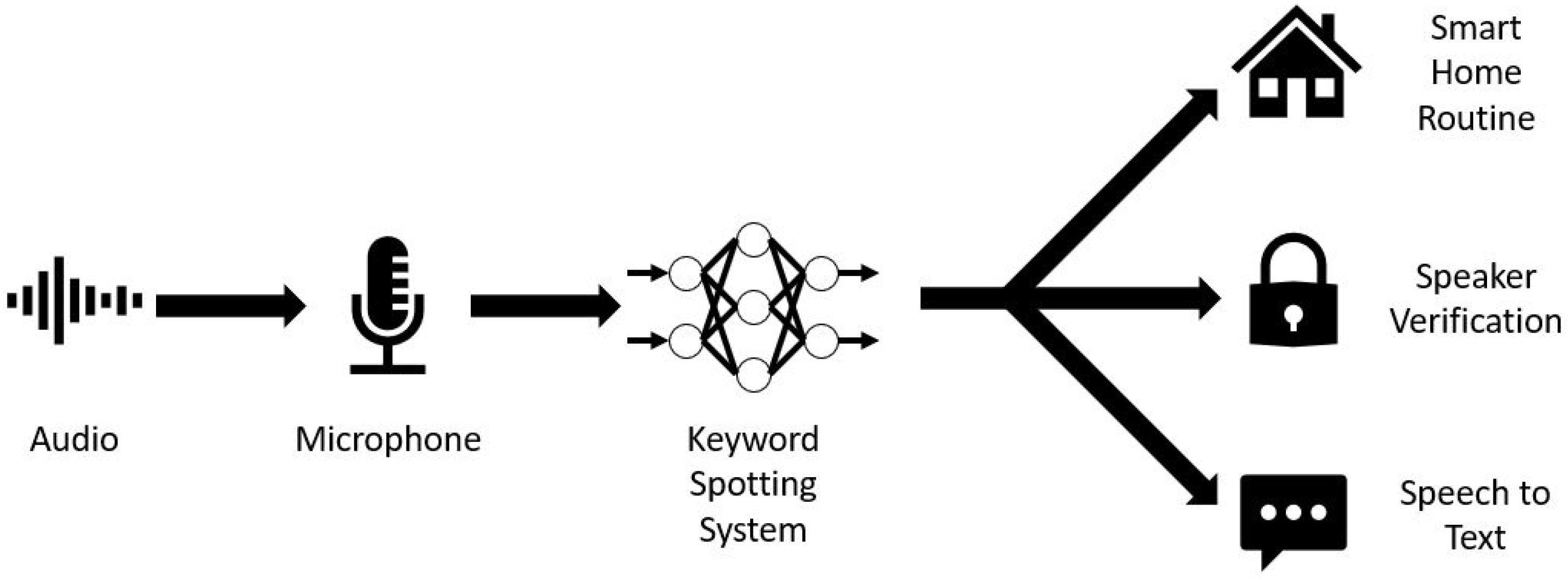
One of the most prominent applications of artificial neural networks in the consumer space is automatic speech recognition in digital assistants. From Amazon’s Alexa [1] and Microsoft’s Cortana [2] to Apple’s Siri [3] and Google’s Assistant [4], voice assistants facilitate a novel method of interacting with electronic devices. Using automatic speech recognition, digital assistants enable users to operate devices simply by speaking commands. Automatic speech recognition has existed since the 1980s using techniques such as Hidden Markov models and Gaussian mixture models. However, it was not until 2012 that artificial neural networks were applied to the problem, substantially improving the user experience and increasing the popularity of digital assistants. Nevertheless, artificial neural networks do not enable full natural language processing models to run on smartphones, smart speakers, and other embedded systems (collectively called edge devices). To fully enable digital assistants, audio data are sent over a network to a server responsible for running the natural language processing neural network, and the results are sent back to the edge device [5]. Constantly processing audio data streams with an artificial neural network does not scale easily with multiple users, and there are privacy and security concerns associated with a device constantly recording audio data. Therefore, the device must recognize a predetermined keyword before sending audio data to the server. This process is called keyword spotting. Even if all the natural language processing could be completed quickly and efficiently on edge devices, privacy and security concerns would still require keyword spotting before running the full speech recognition neural network. Keyword spotting also has applications outside of digital assistants and speech recognition, including smart home automation and speaker verification, which are depicted in Figure 1.
Despite the reduced problem scope of performing keyword spotting on edge devices, significant constraints remain in digital assistant implementations, namely the limited capabilities of the edge device. Generally, embedded systems are limited in two aspects: processing power and memory. For example, the ESP32-WROOM-32E, a popular system-on-a-chip (SoC) for embedded systems, possesses at most two cores operating at 240 MHz with 520 kB of SRAM and 16 MB of SPI flash [6]. Therefore, any neural network running on this SoC must be small enough to fit in the flash storage when inactive and in RAM when running. The SoC must also be able to run the neural network fast enough to avoid losing any words spoken after the keyword. Additionally, if implemented on a more exotic device such as a field-programmable gate array (FPGA), the neural network must fit within the available logic resources, such as flip-flops and lookup tables (LUTs). Developing neural networks for edge devices is not trivial. Google, Apple, Microsoft, and Amazon employ teams dedicated to creating the neural networks powering their respective digital assistants and the proprietary hardware platforms on which the neural networks run. However, designing custom neural network architectures and hardware platforms is infeasible for anyone else. Instead, adapting existing state-of-the-art neural network architectures to inexpensive and widely available edge devices would be more desirable.
Moving more machine learning to edge devices is a fundamental goal within the field of tiny machine learning (TinyML), which began around 2019 [7]. The original motivations were very similar. By moving machine learning tasks to edge devices, applications could reduce latency and data loss while mitigating privacy risks [8]. Since the field’s genesis, researchers have developed techniques such as shrinking, pruning, and quantization for compressing neural networks to run on embedded systems [8]. However, the body of published research within this emerging field is still comparatively small, and most neural network architecture research does not consider the possibility of deployment on edge devices [9,10,11,12]. Furthermore, the research that does consider deployment on edge devices only tests a limited number of models of neural network architectures [13,14,15]. Some research exhaustively explores how a neural network architecture responds to the constraints of edge devices [16], but this is not the norm. Therefore, there is a need for an in-depth investigation of how existing neural network architectures respond to the limitations of embedded systems.
In this research, six distinct neural network architectures (FFCN, DS-CNN, ResNet, DenseNet, Inception, and CENet) are implemented in Python using the TensorFlow machine learning library to investigate the effects of edge device constraints on neural network performance. From these six architectures, 70 neural network models are trained to perform keyword spotting using the Google Speech Commands dataset [17]. Next, each network’s accuracy, memory consumption, model size, and inference latency are evaluated with different quantization methods. It was found that in general, all neural networks architectures after quantization tend to have smaller model size and consume less memory but perform with lower accuracy. However, distinct architectures respond to quantization methods differently—this also depends on their model size. For full-integer quantization, which is the most attractive option for edge devices, the ideal architecture would either be Inception or ResNet, depending on the amount of memory and storage available. After assessing network performance, a neural network model is deployed on an Arduino Nano 33 BLE microcontroller board using TensorFlow Lite for Microcontrollers [18]. The process for generating an RISC-V custom function unit (CFU) for a soft CPU on an FPGA utilizing CFU Playground [19] is also explored. Overall, this research is a preliminary investigation of how a select group of well-known neural network architectures responds to the limitations of embedded systems. Additionally, this research may serve as a guide for designing, training, and deploying neural networks on edge devices for applications beyond keyword spotting.
The main contributions of our work are summarized as follows:
- The complete neural network development process of keyword spotting from implementation, training, quantization, evaluation, and deployment is explored. The implementation and training were carried out with TensorFlow using the well-known Google Speech Commands dataset on a Google Cloud Platform virtual machine. After training, the TensorFlow models were quantized and then converted into smaller, space-efficient FlatBuffers using TensorFlow Lite. The performance metrics, especially those pertinent to edge devices, of various quantization schemes for each neural network model were evaluated. Finally, the steps of deploying the quantized models on embedded systems such as a microcontroller board and an FGPA board were explored through the help of TensorFlow Lite Micro and CFU Playground. This process can be a useful guideline for neural network development on edge devices for keyword spotting and other similar applications.
- A total of 70 models are created, representing different model sizes of six neural network architectures well-suited for keyword spotting on embedded systems. The models are evaluated using metrics relevant to deployment on resource-constrained devices, such as model size, memory consumption, and inference latency, in addition to accuracy and parameter count. CNN-based neural network architectures are chosen for their superior performance in classifying spatial data on edge devices. They are especially fit for our keyword spotting application, as the audio input is processed into mel spectrograms that can be treated as an image-like input. This comparison is helpful for developers to find the best-performing neural network given the constraints of a target embedded system.
- The effect of four available post-training quantization methods in the TensorFlow Lite library on model performance is evaluated. In general, quantization reduces the model size while adversely affecting its performance. However, the reduction in model size and the impact on accuracy, memory consumption, and inference latency varied depending on the neural network architecture as well as the quantization method. This highlights the importance of taking multiple factors, such as network architecture, computing, and memory resources available on the edge device, as well as performance expectations, into consideration for edge computing applications such as keyword spotting.
The rest of this paper is organized as follows. The background and techniques used in this research are summarized briefly in Section 2. In Section 3, the process of this research, i.e., implementation, training, quantization, evaluation, and deployment, is described in detail. The evaluation and deployment results are presented in Section 4. Section 5 summarizes the whole paper.
2. Background
In a basic keyword spotting system, a microphone first records an audio signal. The audio data are then processed to extract high-level features, allowing the neural network to better differentiate between keywords. The neural network then processes the extracted features. Finally, the neural network produces a prediction. This prediction is a probability vector, with each element indicating the likelihood that the audio signal matched a different keyword.
2.1. Audio Processing
One of the most critical steps in neural network development is preparing the training data. This step may be further broken down into two smaller steps: finding a suitable dataset and extracting features. The selected dataset must contain the relationship, pattern, or function that the neural network will learn. In the case of keyword spotting, this means finding a suitable collection of audio clips of people saying the desired keywords. This dataset is then processed to extract features before training a neural network.
The Google Speech Commands dataset [17] is selected for training neural networks in this research. This dataset consists of 105,829 one-second audio recordings of 35 keywords, saved as 16-bit 16 kHz PCM Wave files. Since the dataset was collected through volunteer submissions, participants were not obligated to submit recordings of every keyword. Therefore, the number of recordings for each keyword varies. Nevertheless, the size of this dataset, in conjunction with the limited vocabulary, makes it an attractive choice for training neural networks for keyword spotting applications.
A feature is a particular type of information on which the neural network is trained. In this research, the Wave files are processed into mel spectrograms that contain high-level features of the audio signal. Specifically, the short-time Fourier transform is first applied to the audio amplitude values to produce a spectrogram, which depicts the change in the power of different frequency components throughout the original audio. This allows the neural network to focus on classifying the higher-level spectrogram [20]. Additionally, the spectrogram can be treated as an image-like input rather than a sequence of amplitude values. Since humans perceive volume and frequency logarithmically rather than linearly, the spectrogram is further processed into a corresponding mel spectrogram with amplitude values converted to the decibel (dB) scale and frequency values converted to the Mel scale through a series of overlapping triangular filters in the frequency domain [20]. In our research, a mel filter bank with 40 filters is implemented.
Please note that another feature representation, called mel-frequency cepstral coefficients (MFCCs), is also used often in speech recognition applications. The goal of MFCCs is to extract highly unrelated coefficients from the mel spectrogram through the discrete cosine transform [21]. While MFCCs provide a compact, high-level representation of the original audio recording, decreasing the computation required of the neural network, the increased network efficiency comes at the cost of increased preprocessing. Therefore, the target platform’s resources and the neural network’s use case must be considered when deciding which representation to use, especially when the desired use case is keyword spotting on low-power edge devices. In this research, the mel spectrogram feature is used.
2.2. Selected Neural Network Architectures
After finding a suitable dataset and selecting a preprocessing method to extract features, the data are ready to be utilized by a neural network for training. Neural networks can largely be categorized into a few classes based on their architecture. Some of these classes include convolutional neural networks (CNNs), feedforward fully connected neural networks (FFCNs), recurrent neural networks (RNNs), and generative adversarial neural networks (GANs). This paper specifically concentrates on CNN-based architectures because of their reputation for having compact model sizes, making them suitable for low-power applications [22]. In addition, there are also readily available implementations for CNNs in popular deep learning frameworks, such as TensorFlow. While it has been shown that CNN-based architectures outperform FFCNs in keyword spotting with far fewer parameters [22], FFCNs are still implemented as a baseline when evaluating the performance of other CNN-based architectures. GANs are excluded here because keyword spotting is a discriminative rather than a generative task. In other words, GANs are designed to generate some new output rather than classify an input. Additionally, RNNs are passed over, as they are better suited to processing temporal or sequential data, while CNNs are superior at processing spatial data (such as an image or mel spectrogram).
Six neural network architectures were investigated: FFCN [9], DS-CNN [23], ResNet [11], DenseNet [12], Inception [10], and CENet [14]. While the FFCN architecture was selected mainly for a baseline comparison, the other neural network architectures were chosen for their performance in image classification or keyword spotting tasks. It should be noted that the networks tested in this research do not exactly follow the descriptions in their original publications. Rather, they required minor adaptations to accommodate the size of the inputs and a smaller training dataset.
- FFCN: The FFCN has a simple network architecture with one input layer, one output layer, and an arbitrary number of layers in between, called hidden layers. FFCN models exhibit a noticeable leap in performance over hidden Markov model (HMM)-based approaches in keyword spotting tasks [9].
- Depthwise separable convolutional neural network (DS-CNN): The DS-CNN was designed for efficient embedded vision applications [23]. The DS-CNN effectively decreases both the number of required parameters and operations by replacing standard 3D convolution layers with depthwise separable convolution layers (i.e., 2D depthwise convolutions followed by 1D pointwise convolutions), which enables the utilization of larger architectures, even in embedded systems with limited resources.
- Deep residual network (ResNet): The ResNet architecture was conceived to combat the vanishing gradient problem, i.e., despite the neural network growing in size with each additional layer, the accuracy saturates and then degrades rapidly. Residual connections and the residual building block were devised to solve this problem. In a residual block, the output of a layer is added to another layer deeper in the block. This addition is followed by applying a nonlinear activation function to introduce nonlinearity into the block. Chaining these residual layers together (using convolution layers for the weight layers) forms a ResNet neural network. ResNet was originally proposed for image recognition [11]. It has also been applied to keyword spotting with the flexibility to adjust both the depth and width for a desired trade-off between model footprint and accuracy [24].
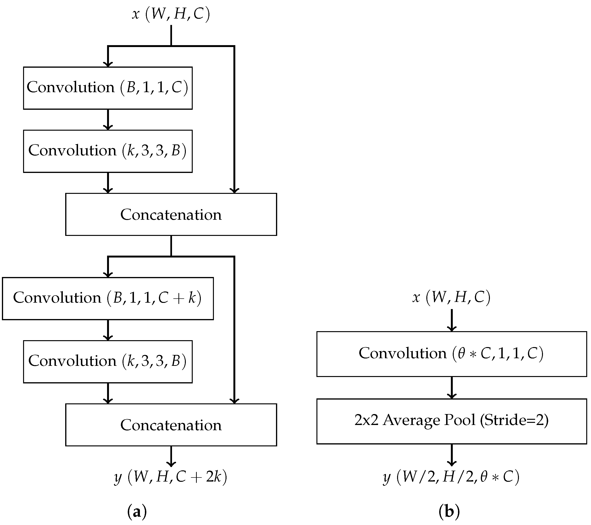
- Dense convolutional network (DenseNet): DenseNet also combats the vanishing gradient problem by promoting effective feature propagation. It requires a comparatively smaller number of parameters and fewer computations, making it well-suited for embedded applications. The DenseNet architecture implements a concept similar to residual connections with the introduction of the dense block. In short, a dense block is a series of alternating convolution and concatenation operations where the input to each convolution layer is the combined output of every preceding convolution layer [12]. Thus, each layer passes its own feature maps to all subsequent layers. Dense blocks do not reduce the dimensions of feature maps due to the presence of concatenation operations. Thus, transition layers are inserted between dense blocks, where each transition layer consists of a convolutional layer followed by pooling. The DenseNet architecture has two other variations: DenseNet-B and DenseNet-C [12]. DenseNet-B introduces bottleneck layers, which are inserted before convolution layers within dense blocks to reduce the number of feature maps and thus reduce the total number of weights. DenseNet-C introduces a compression factor as part of transition blocks to reduce the number of feature maps passed between dense blocks. DenseNet-B and DenseNet-C may be combined to form DenseNet-BC to prevent the number of parameters from ballooning. Figure 2 shows examples of a dense block and a transition block in DenseNet. In these figures, W, H, and C in represent, respectively, the width, height, and the number of channels of the input matrix x. The same notation applies to the output y. Each convolution block, e.g., Convolution , uses N convolution kernels, each with a size of width height channels , and produces N output feature maps. B in Figure 2a represents the number of feature maps produced by the bottleneck layer in DenseNet-B.
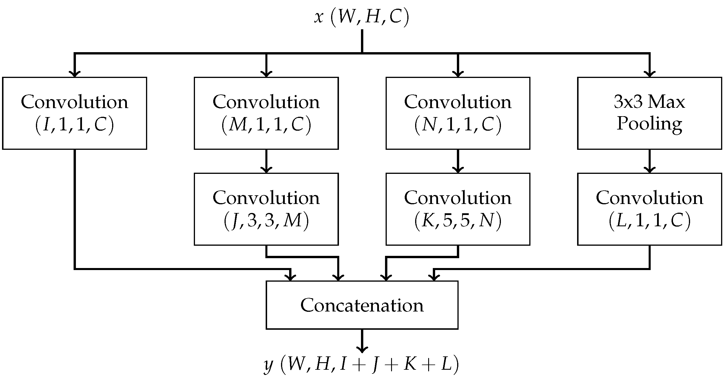
- Inception: The Inception architecture was designed to address two problems associated with increasing convolutional neural network size: the increase in the number of parameters and the amount of computational resources required to produce a result. These problems share a solution: sparsity, i.e., by replacing all fully connected layers with sparsely connected layers. However, due to limitations in modern computer architecture, sparse calculations are very inefficient. Thus, the Inception module was developed to approximate these sparse layers while maintaining reasonable efficiency on modern computers. An Inception module is composed of a series of parallel convolutional layers with different filter sizes (1 × 1, 3 × 3, 5 × 5) and a pooling layer [10]. With multiple filter sizes, the network is enhanced to capture features at different levels of abstraction. Chaining these modules together then forms an Inception neural network. The structure of an Inception module is depicted in Figure 3.Inception was originally designed for image classification and detection [10], and there is no known previous work applying it to keyword spotting. However, it is reasonable to apply Inception to the speech recognition problem, since a mel spectrogram is a pictorial representation of an audio recording.
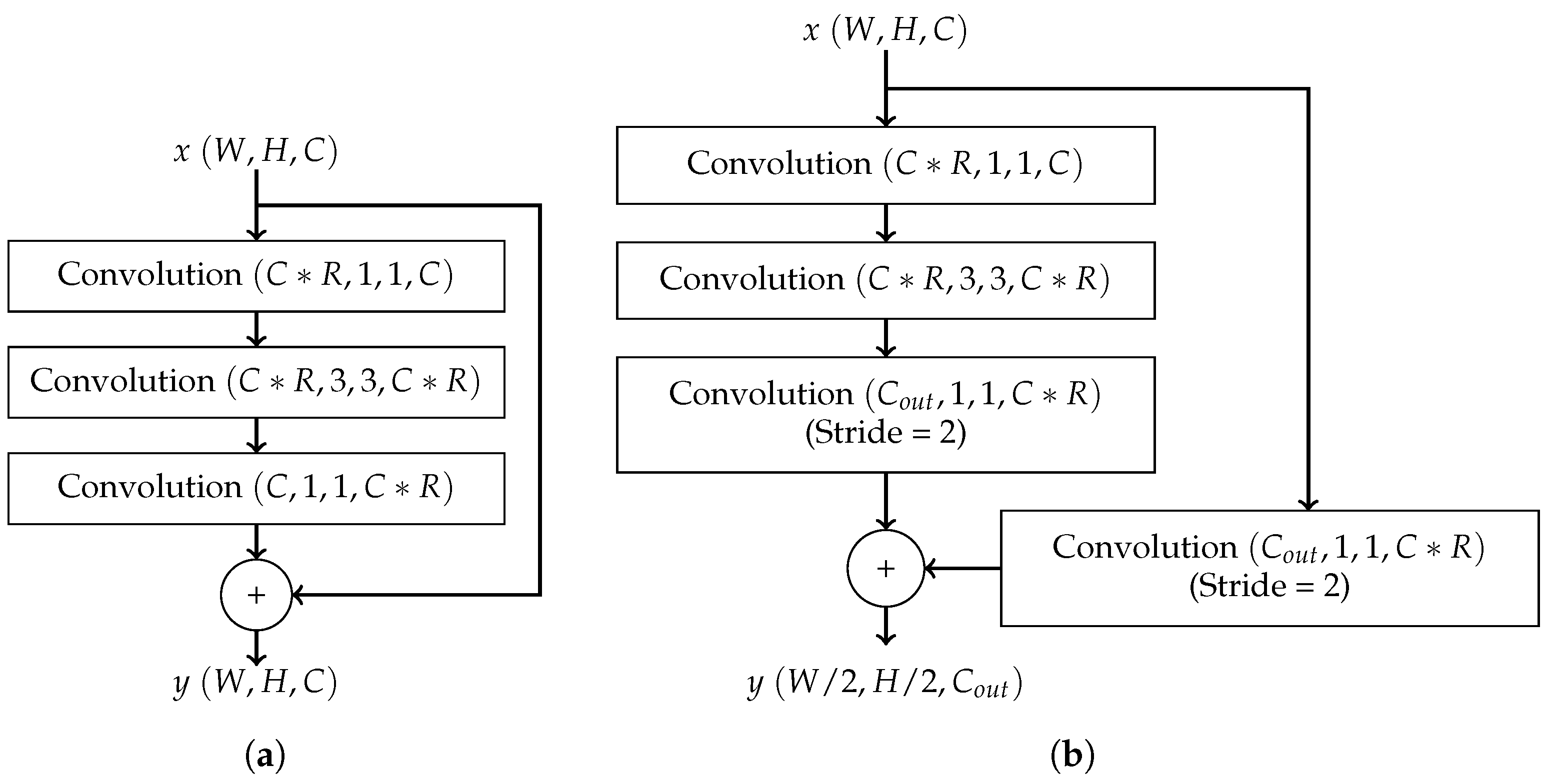
- CENet: To enable execution on embedded systems, CENet employs a residual bottleneck block. These bottleneck layers are connected to form a stage, and multiple stages can be chained together to form a complete network. As the bottleneck blocks do not decrease the size of the feature maps, a residual connection block is required to transition between stages. Each connection block decreases the number of internal feature maps by a factor of to lower resource requirements. These connection layers are inserted between stages of bottleneck blocks, forming a complete network. Figure 4 illustrates the structures of a residual bottleneck block and a residual connection block in CENet. The CENet architecture was designed explicitly to perform keyword spotting on resource-constrained devices. The proposed residual connection and bottleneck structure is compact and efficient and shown to generate superior performance [14].
2.3. Quantization
Neural network quantization emerged as a technique to facilitate the deployment of neural network models on embedded systems [25]. Using quantization, operations and weights are stored using fewer bits than those used during training. For example, while a neural network has been trained using 32-bit floating-point weights and operations, the network may be saved and deployed using 16-bit floating-point values or 8-bit integers. By decreasing the precision of the weights and operations, the amount of space required to store the model also decreases. Additionally, an embedded system running a neural network may save power and reduce latency as a result of the quantization process, since some embedded systems lack the hardware acceleration provided by a dedicated floating-point unit.
There are two main methods of quantization: quantization-aware training (QAT) and post-training quantization (PTQ) [25]. During QAT, a neural network model must be trained so that the quantization noise is also modeled during the training process. While QAT can find optimal solutions for a given quantization level, especially for more extreme quantization schemes, QAT cannot reuse any previous training completed using floating-point values. In contrast, PTQ may be applied to a neural network without retraining. At most, PTQ requires a representative dataset for calibration.
3. Method
The complete research process is separated into several distinct phases: implementation, training, quantization, evaluation, and deployment, as depicted in Figure 5. During the implementation phase, the code creating the datasets and defining the neural network architectures was written. During the training phase, neural networks from each of the architectures were trained to perform keyword spotting. During the quantization phase, the trained models were converted to smaller models using various quantization schemes. During the evaluation phase, the trained neural networks were evaluated for number of parameters and model size. Performance metrics of accuracy, memory consumption, and inference latency were also measured for different quantized models. Finally, a neural network was tested on an embedded system and an FPGA.
3.1. Dataset Implementation
The first section of code is the function for creating the training and validation datasets. This function reads the Google Speech Commands dataset [17]. The validation_split parameter determines the number of samples in each dataset. Within these datasets, samples are grouped into batches, the size of which is determined by the batch_size parameter. The code then converts the one-second audio clips into mel spectrograms using the sample_rate, nfft, step_size, mel_banks, and max_db parameters. After considering the memory, power, and computational constraints of embedded systems, the datasets were created using the parameter values listed in Table 1.
Running the dataset creation function with these parameters yielded two datasets: one for training and one for validation. Within each dataset, audio samples were grouped into batches of 128, and the one-second audio clips were transformed into 40 × 40 mel spectrograms, each representing 25 ms of audio input.
3.2. Architecture Implementation
Each of the six neural network architectures was implemented as a class, allowing for different models to be created, tested, and modified easily. Each model has one input layer, one fully connected output layer, and various numbers of hidden layers. The input layer accepts a 40 × 40 mel spectrogram of an audio sample from the dataset. The output layer is a vector of 35 probabilities indicating the likelihood of the input belonging to each keyword category. After considering the number of parameters and layers, the required training time, and the shape of the input and output layers, multiple models for each neural network architecture were selected. Specifically, 5 FFCN models, 9 DS-CNN models, 6 ResNet models, 20 DenseNet models, 8 Inception models, and 22 CENet models were selected for testing, with an overall total of 70 models tested. All the convolutions and fully connected layers use the ReLU activation function. The softmax function is used in the output layer to produce a vector of probabilities for each classification category. The implementation and parameters associated with each model are explained in Appendix A.
3.3. Training
After writing the code for the dataset and neural network architectures, each model was trained using TensorFlow [26] on a Google Cloud Platform [27] virtual machine with a quad-core CPU and NVIDIA Tesla T4 GPU running Debian Linux. First, each model was created using one of the six neural network architecture classes. The model was then compiled to use the Adam optimizer [28] with a learning rate of 0.001 and the sparse categorical cross-entropy loss function. The model was also compiled with the accuracy metric flag so that TensorFlow would track the model’s accuracy during training. Finally, the model was trained with the training and validation datasets. The model was trained for 100 epochs. The training process was also configured to save the model after every epoch and write the model’s current accuracy to a log file. This process was repeated for each of the 70 neural network models.
3.4. Quantization
After training, each neural network was evaluated in terms of model size, number of parameters, latency, memory consumption, and accuracy using different quantization methods. TensorFlow Lite [29] facilitates the conversion of large TensorFlow models into smaller, space-efficient FlatBuffers. This converted model can easily be deployed on resource-constrained systems. The performance of the converted TensorFlow Lite FlatBuffer models was evaluated with four available post-training quantization methods: 16-bit floating-point quantization, dynamic range quantization, integer quantization with floating-point fallback, and full-integer quantization [30].
- The 16-bit floating-point quantization utilizes 16-bit floating-point values for weights and 32-bit floating-point values for operations.
- Dynamic range quantization allows the model to mix integer and floating-point operations when possible (falling back to 32-bit floating-point operations when necessary) while the weights are stored as 8-bit integers. The weights are quantized post training, and the activations are quantized dynamically at inference in this method.
- Integer quantization with floating-point fallback utilizes integers for weights and operations. If an integer operation is not available, the 32-bit floating-point equivalent is substituted. This results in a smaller model and increased inference speed. For convenience, this scheme is shortened hereafter as integer-float quantization.
- Full-integer quantization utilizes only 8-bit integers for weights and operations, removing the dependency on floating-point values. This method achieves further latency improvements, reduction in peak memory usage, and compatibility with integer-only hardware devices or accelerators.
After the TensorFlow Lite models were saved, the accuracy, memory consumption, latency, and size of the model files were recorded. The collected results were saved in a CSV file and evaluated on the same Google Cloud Platform virtual machine. The evaluation results are presented and elaborated in Section 4.
3.5. Deployment
After evaluating the neural network models, one of the neural networks (specifically DS-CNN model 8 in Table A2) was tested on two embedded systems: an Arduino Nano 33 BLE microcontroller board and a Digilent Nexys 4 FPGA board. The Arduino Nano 33 BLE microcontroller board has a 64 MHz Arm Cortex-M4F processor with 1 MB of flash storage, 256 kB of RAM, and a microphone [31]. The Digilent Nexys 4 FPGA board features a Xilinx Artix-7 FPGA with 15,850 logic slices and a microphone [32]. In both cases, TensorFlow Lite Micro was utilized in the deployment process. Unlike normal computers, embedded systems do not always have operating systems and have much tighter power, performance, and memory constraints. TensorFlow Lite Micro was designed to run neural networks within these stricter limitations [18].
The deployment of the converted TensorFlow Lite FlatBuffer models onto the Digilent Nexys 4 FPGA board was carried out through CFU Playground [19]. CFU Playground facilitates the generation of custom function units (CFUs) that implement custom machine learning instructions, which accelerate a neural network running on a soft RISC-V CPU on an FPGA. Among other benefits, these CFUs can optimize machine learning operations utilizing constant operands, perform more computations in parallel, reduce data movement, and perform multiple operations simultaneously. This CFU Playground project produces a full RISC-V soft CPU to accelerate custom instructions as defined in cfu.h and cfu.py. By adding and defining custom instructions in these files, they can be used elsewhere in the project, accelerating the neural network.
4. Evaluation and Deployment Results
After collecting data from each neural network, the performance of the architectures without quantization and with different quantization schemes was evaluated. Furthermore, a DS-CNN model was also deployed and validated on the Arduino Nano 33 BLE microcontroller board and the Digilent Nexys 4 FPGA board.
4.1. Evaluation Results
The parameter count, accuracy, memory, and inference latency versus model size for each quantization scheme described in Section 3.4 were evaluated for all the implemented neural network architecture models. Please note that the amount of memory consumed by each model was measured by the TensorFlow Lite benchmark tool [29]. The numbers measured should not be considered accurate if the model is deployed on an embedded system. This is because the TensorFlow Lite benchmark tool itself affects the memory footprint. As a result, the measurement value is only approximate to the actual memory footprint of the model at runtime. Additionally, the measurement for peak memory usage was obtained via polling every 50 ms, so the measurement’s accuracy is also limited by the polling rate. Nevertheless, these results provide a useful point for comparison.
4.1.1. Performance without Quantization
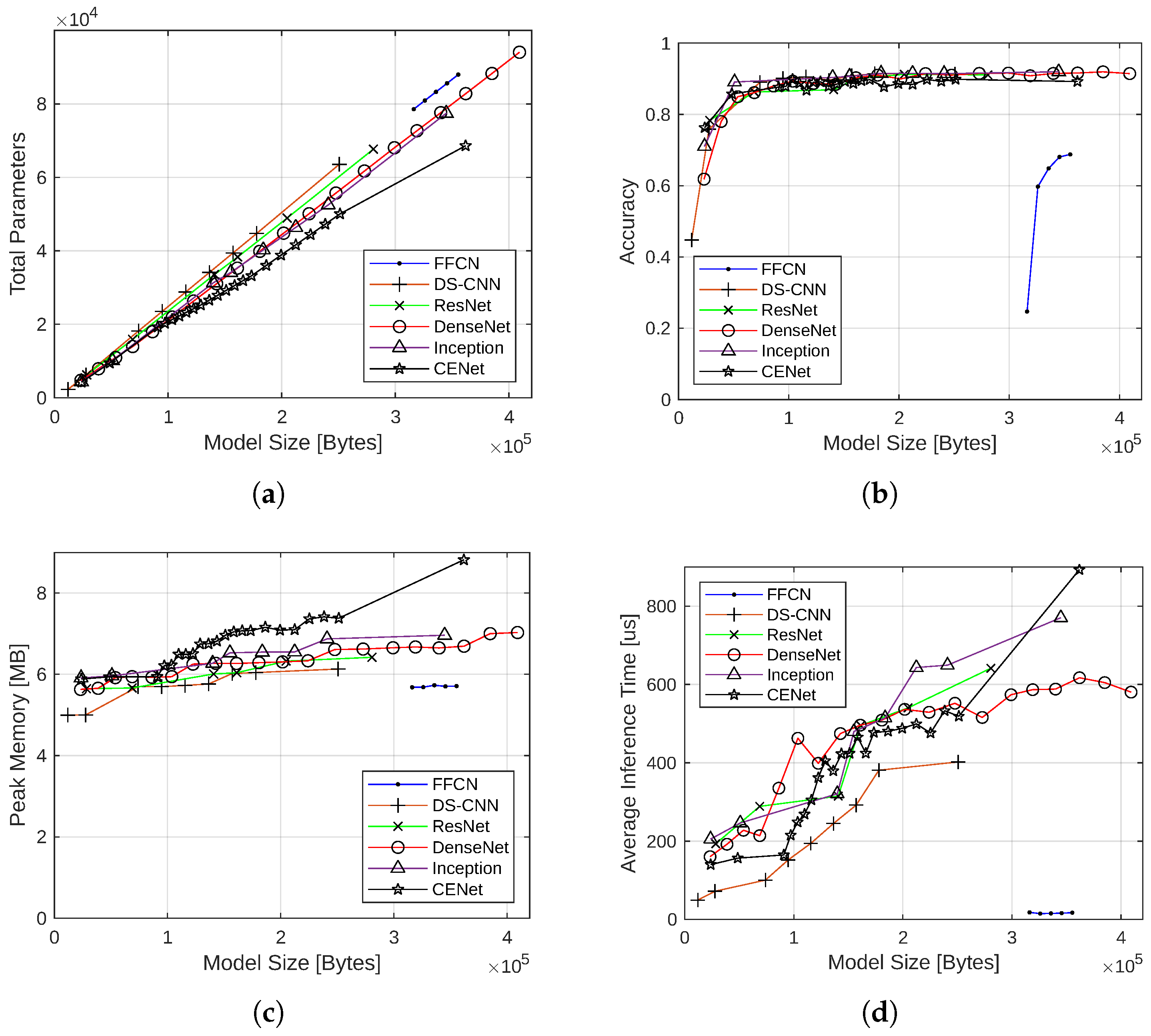
The performance of various neural network architectures was first compared with no quantization. These models utilized 32-bit floating-point values for weights and operations, making them equivalent to the original trained TensorFlow models. The 70 nonquantized models were first grouped by architecture and plotted according to the model size in bytes (i.e., size of the FlatBuffer file for each TensorFlow Lite model). The number of parameters for each model, as well as the accuracy, memory consumption, and inference latency after training for 100 epochs are depicted in Figure 6. These data are used as a baseline to evaluate the effect of different quantization schemes on keyword spotting performance with a certain neural network architecture.
For all architectures, the number of parameters was strongly correlated with the model size. This result was expected, but the more interesting insight is the slope of each of the lines, indicating the parameter density of the model. FFCN had the highest slope, followed by DS-CNN, ResNet, DenseNet, Inception, and CENet. By knowing the parameter density of the architectures, a developer knows which architecture will allow the greatest number of parameters within a given amount of memory.
In terms of accuracy, the architectures performed similarly, except for the FFCN architecture. Above model sizes of 50 kB, the architectures achieved upward of 90% accuracy, with Inception peaking at 91.95%. However, the accuracy of each architecture dropped significantly with model sizes smaller than 50 kB. At approximately 25 kB, the maximum accuracy was 78.34% (ResNet), with a minimum of 61.83% (DenseNet). The DS-CNN architecture produced the smallest model (11,968 bytes), but this diminutive size came at the cost of accuracy (44.78%). The lackluster performance of the FFCN architecture was expected, as FFCNs require more layers and parameters to approximate the performance of CNNs in image classification tasks. The accuracy of the FFCN architecture can be improved with more hidden layers or more neurons in each layer; however, this results in a significant increase in the model size, surpassing the sizes of other architecture models being compared. Overall, the accuracy of each architecture quickly plateaued as model size increased. This plateau was likely caused by a relatively short training time of 100 epochs. It is not uncommon for neural networks to train for thousands of epochs before reaching their peak accuracy [11]. More differentiation could have been observed in the larger neural networks by allowing for additional training time.
All the architectures consumed similar amounts of memory. Generally, CENet models consumed more memory than models of other architectures with a similar size, followed by Inception, DenseNet, ResNet, DS-CNN, and FFCN. Each architecture’s memory consumption increased roughly linearly with model size, corresponding to the increased space required to hold the intermediate feature maps and parameters in memory.
For inference latency, FFCN was the clear winner, achieving an average inference latency of 15.038 s. DS-CNN was the runner-up, achieving a lower inference latency than models of other architectures with similar sizes. Beyond FFCN and DS-CNN, no architecture was unequivocally better than another. Generally, average inference latency increased linearly with model size. The deviations from this linear trend have a few plausible explanations. The computer running the benchmark could have a better CPU cache hit rate, resulting in fewer reads from main memory and lower inference times. The CPU clock rate could have fluctuated during the benchmark. The branch predictor in the CPU could have a better prediction rate for certain models. Regardless of the exact reason, the average inference latency measurements are still useful for illustrating how each architecture’s inference latency responds to changes in model size.
4.1.2. Model Size Reduction with Quantization
With the implementation of various quantization schemes, the model sizes, in terms of the size of the TensorFlow Lite model stored in a FlatBuffer file, were reduced. The average model sizes of each architecture with the four different quantization schemes as compared with the corresponding nonquantized model size are listed in Table 2.
It should be pointed out the neural network model stored in a FlatBuffer file contains more than just the weights. Other information, such as the computational graph of the model, operations involved, and dequantization method from weights and scales are also included. Therefore, a perfect 2× reduction in files size with the 16-bit floating-point quantization scheme is not observed for most architectures, although the weights themselves should occupy only half the size as before. The same reason applies to other quantization schemes as well. Nevertheless, it can be seen that different architectures cause different levels of model size reduction. The file size reduction is close to the theoretical weight size reduction only for the architectures with very simple structures, e.g., FFCN.
4.1.3. Effect of Quantization on Accuracy
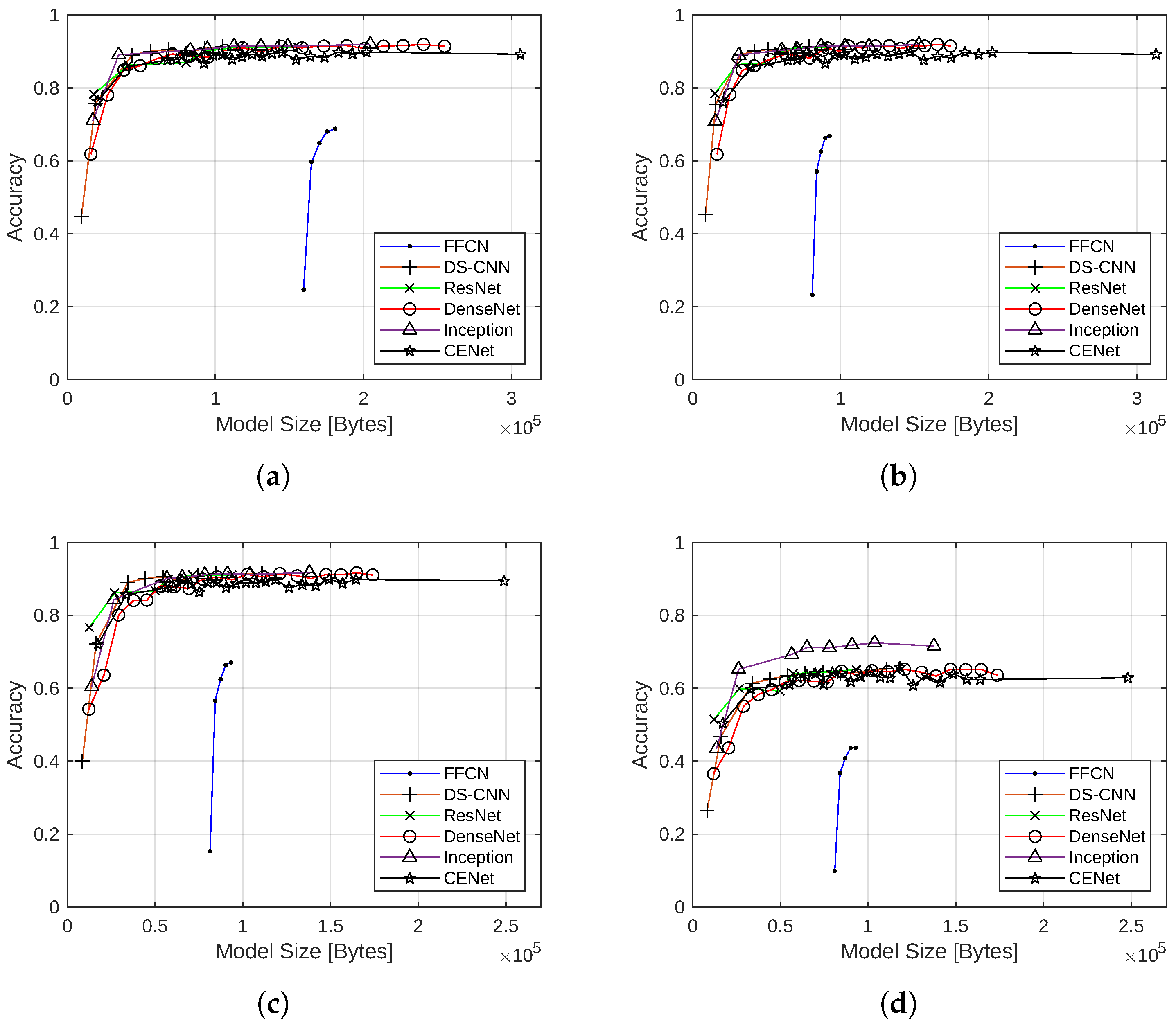
To evaluate the impact of quantization schemes on accuracy, the inference accuracy versus model size for each neural network architecture after training for 100 epochs were plotted under the four different quantization schemes in Figure 7.
Overall, the models with the 16-bit floating point, the dynamic range, and the integer-float quantization schemes closely mimicked their nonquantized counterparts in terms of accuracy, with reduced model sizes. For 16-bit floating-point quantization, this is likely due to the simplicity of converting 32-bit floating-point values to 16-bit floating-point values with minimal error. The ability of the dynamic range and the integer-float quantization models to provide the benefits of 8-bit integer quantization with best effort post training or at inference while avoiding the associated drop in accuracy was a pleasant surprise. For model sizes above 30 kB, most architectures, except FFCN, still exceeded 90% accuracy. For model sizes smaller than 30 kB, however, a drop in accuracy was observed. Compared with the nonquantized models, the accuracy achieved with 16-bit floating-point quantization and dynamic range quantization is about the same, whereas the drop in accuracy is more pronounced for models with integer-float quantization. For example, the smallest ResNet model achieves 76.67% accuracy under the integer-float quantization, which is more a than 1.5% reduction from 78.34% with no quantization. For the smallest DenseNet model, the accuracy dropped from 61.83% without quantization to 54.24% with integer-float quantization.
The full-integer quantization scheme greatly impacted the performance of the models, with an approximate 20% drop in accuracy. The drop in accuracy was likely caused by the limitations of PTQ. While PTQ aims to maintain network performance using a representative dataset for calibration, some inaccuracies are inevitably introduced by converting all 32-bit floating-point values to 8-bit integers. QAT could achieve better results, but the model would have to be completely retrained.
Although the FFCN models with the quantized schemes have lower accuracy than all the CNN-based architectures, they have other advantages, such as less memory consumption, lower inference latency, and greater size reduction with quantization. It has also been discovered that FFCN accuracy can be improved with pooling [15]. Therefore, enhanced FFCN models may still be considered for certain keyword spotting applications on embedded systems.
4.1.4. Effect of Quantization on Memory Consumption
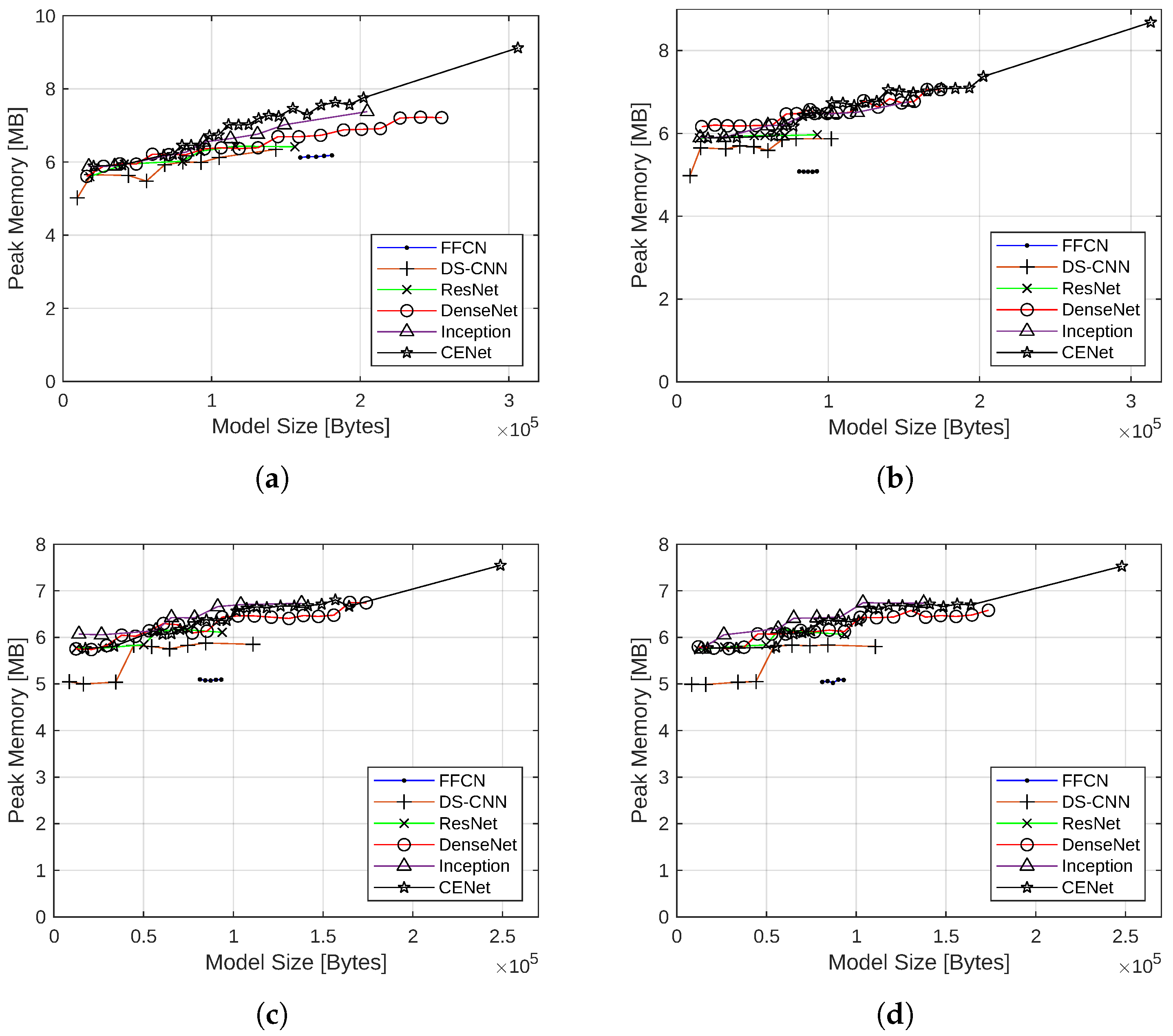
The peak memory consumption as measured by the TensorFlow Lite benchmark tool for the neural network models with the four quantization schemes is shown in Figure 8.
CENet produced the model with the largest memory footprint, with peak memory consumption of the largest model varying between 85.4% with full-integer quantization to 103.5% with 16-bit floating-point quantization, as compared with the memory consumption without quantization. DS-CNN produced the model with the smallest memory footprint, with peak memory consumption very close to that of its nonquantized counterpart. In general, DS-CNN and FFCN models require less memory than other architecture models. These results, including the order of memory consumption of different architectures, closely followed the nonquantized models. Each architecture’s memory consumption increased roughly linearly with model size, corresponding to the increased space required to hold the intermediate feature maps and parameters in main memory.
When the quantization schemes are considered, the peak memory consumption slightly decreases with the quantization schemes in the following order: 16-bit floating point, dynamic range, integer-float, and full integer.
4.1.5. Effect of Quantization on Inference Latency
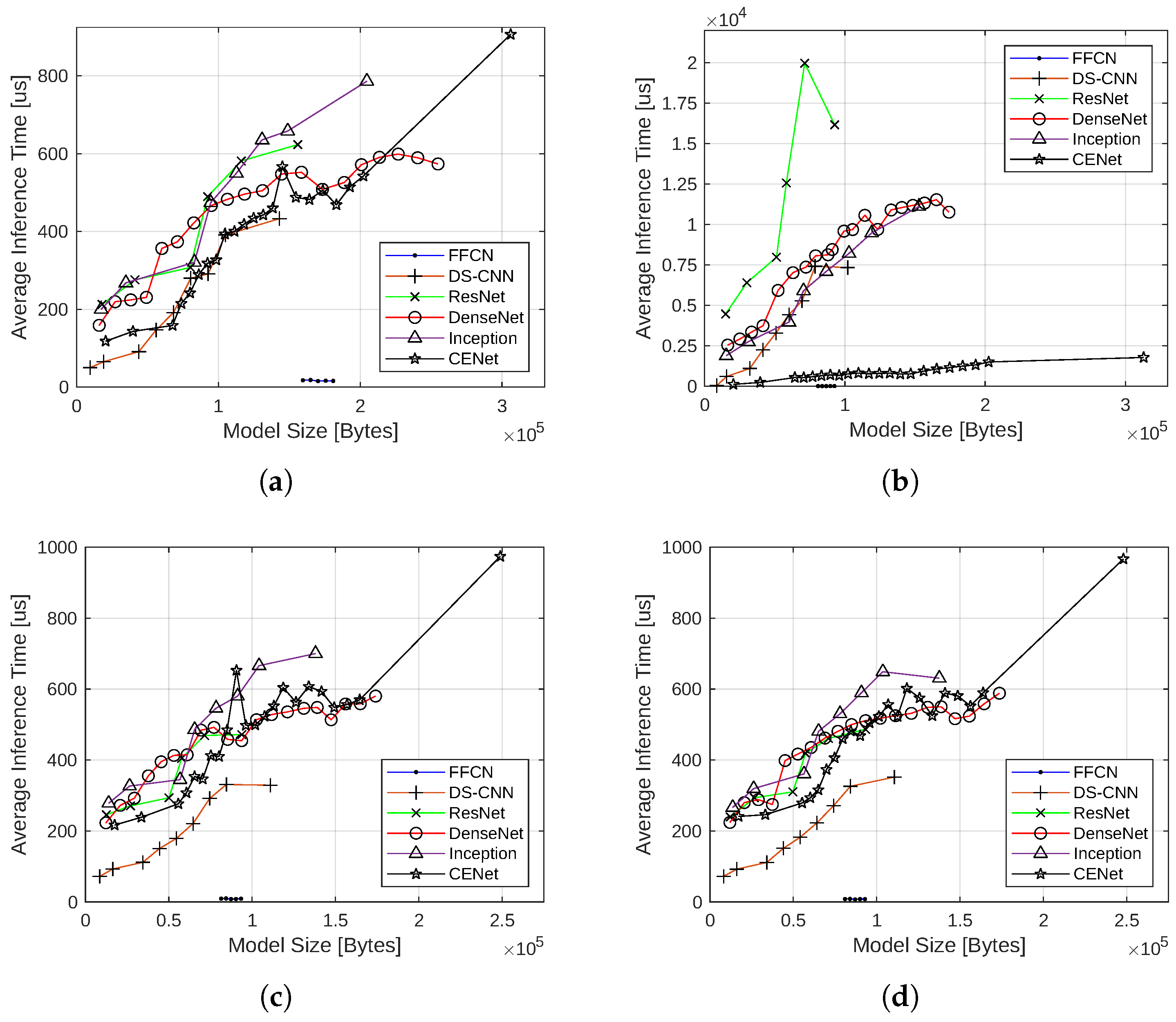
The inference latency of the neural network models with the four quantization schemes is shown in Figure 9.
Like the nonquantized versions, the FFCN architecture was the clear winner. Beyond FFCN, no architecture was unequivocally better than another. However, each architecture exhibited the same linear trend in every quantization method. The deviations from the linear trend also have the same hardware-related explanations (number of memory reads/writes, CPU clock rate, and CPU branch predictor hit/miss rate).
The average inference latency of the 16-bit floating point, integer-float, and the full-integer quantization models was very close to the nonquantized models, presumably due to the lack of runtime quantization. However, inference latency increased significantly with dynamic range quantization compared with the other quantization methods. This increase in latency may be due to the additional operations required to quantize operations at runtime. This increase in inference time is the most significant in ResNet but comparatively less in CENet.
4.1.6. Summary
Overall, each architecture’s relative performance varied depending on the model size and quantization method. The nonquantized models were always the largest in both model size and memory consumption, followed by 16-bit floating-point quantization, dynamic range quantization, integer-float quantization, and full-integer quantization. The DS-CNN architecture consistently produced the smallest model size. In terms of memory consumption, DS-CNN and FFCN models consistently utilized less memory than similar-sized models of other architectures.
While the architectures performed similarly in accuracy, ResNet consistently distinguished itself as the most accurate architecture when model sizes approached their minimum. For the larger models, accuracy clustered around 90%, except for the full-integer quantization models. Additionally, with full-integer quantization, Inception achieved over 70% accuracy, outperforming all other architectures by approximately 10%, with model sizes larger than 25 kB.
In terms of latency, all neural networks, except those using dynamic range quantization, could complete inference in less than 1 ms. Additionally, latency and model size were positively correlated. While latency is an important metric to consider when evaluating a neural network, no architecture was inadequate. For this keyword spotting application, 25 ms would pass before a new mel spectrogram could be produced, meaning that all models would easily complete the inference process before a new spectrogram was available.
Finally, the number of parameters increased linearly with model size, as expected. However, each architecture exhibited different parameter densities (the number of parameters per byte of model size or the slope of the parameter count versus model size graph). Since the number of model parameters is correlated with the flexibility of a neural network, this comparison may be helpful when training a neural network using a dataset much larger than Google Speech Commands.
Since the processor within an edge device may not always have a floating-point unit, full-integer quantization is the most attractive option. Otherwise, the latency of the neural network would significantly increase by attempting to compute floating-point operations completely in software. Considering this, the best architecture would be Inception or ResNet, depending on the memory and storage available.
4.2. Deployment Results
4.2.1. Deployment on Arduino Nano BLE Microcontroller Board
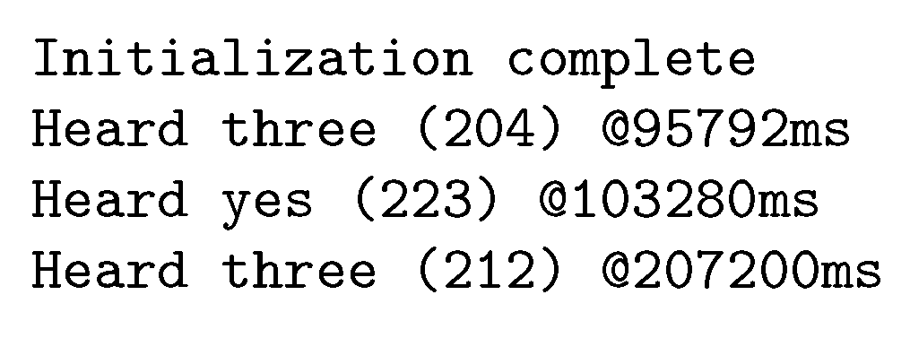
To deploy the neural network on the Arduino board, the keyword spotting example (i.e., micro speech directory) provided in the TensorFlow Lite Micro Arduino Examples repository [33] was modified. After the trained DS-CNN model was loaded, an initial reshaping layer was added to the model input, such that the expected input shape was a 1-D rather than a 2-D array. The modified model was then requantized using full-integer quantization and saved. The quantized model was subsequently converted into a byte stream and inserted into the file that holds the model features in the Arduino project. In addition, the main setup function was modified to include the necessary operations in the ops resolver and increase the arena size accordingly (i.e., to 102,400 bytes for holding the memory the DS-CNN model needed for execution). The list of keywords in the Google Speech Commands dataset, as well as other features such as slice size, count, stride and duration, were also included in the model settings header file. After making these modifications, the Arduino project was compiled and downloaded to the board. Once finished, the serial monitor was opened to verify the neural network’s functionality.
A printout of the inference output shown on the serial monitor is included in Figure 10. While the accuracy of this model was lacking, it successfully performed keyword spotting and ran without exceeding the limited available resources (256 kB RAM and 1 MB flash).
4.2.2. Deployment on Digilent Nexys 4 FPGA Board
The same neural network was tested on a Digilent Nexys 4 FPGA board using CFU Playground [19]. Similar steps in Section 4.2.1 were followed to modify the corresponding files and settings in the micro_speech directory for the DS-CNN model. Additionally, the models.c file was edited to include the new DS-CNN model. Finally, the tflite.cc file was edited to specify the amount of memory the DS-CNN model needed for execution.
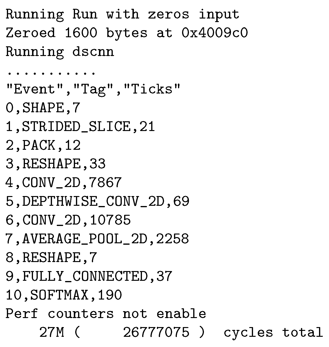
After making the changes, the project was synthesized, compiled, and downloaded to the Digilent Nexys 4 FPGA board. The terminal then displayed a menu, with an option to test the DS-CNN model by feeding the network zeros. After finishing the inference process, a report was displayed in the terminal. The report consisted of two parts: a summary of the inference process (e.g., as shown in Figure 11) and the output of the neural network (with a score calculated by the neural network model for each of the 35 classes).
The summary in Figure 11 lists the neural network operations that were executed along with the number of ticks required to complete each operation. In this context, a tick is equal to 1024 clock cycles. The total number of clock cycles (i.e., 26,777,075) required for one inference is also included in the result. Since the clock signal frequency was 75 MHz, the total time required for one inference was 357.028 ms.
5. Discussions and Conclusions
In this paper, an example of the complete neural network development process has been demonstrated. First, six neural network architectures (FFCN, DS-CNN, ResNet, DenseNet, Inception, and CENet) were implemented in Python using the TensorFlow machine learning library. These architectures were modified slightly from the descriptions in their original papers to accommodate the requirements of keyword spotting. Of these 6 architectures, 70 models were created and trained using the Google Speech Commands dataset for 100 epochs on a Google Cloud Platform virtual machine. After training, each model was subjected to different quantization methods, creating a total of 350 different models. Next, model size, number of parameters, accuracy, memory consumption, and inference latency of the trained and quantized models were measured to observe how each architecture responded to progressively tighter resource constraints. After evaluating the models, a single DS-CNN model with full-integer quantization was deployed on an Arduino Nano 33 BLE microcontroller board using TensorFlow Lite for Microcontrollers. While the model had to be wrapped and requantized to accept a differently shaped input, deployment was relatively seamless, as an existing keyword spotting example could be modified. The model was also tested on the Digilent Nexys 4 FPGA board. Using CFU Playground, a RISC-V CFU was generated to accelerate the neural network.
This research could be continued by implementing and training more neural network architectures and investigating the impact of training beyond 100 epochs. Additionally, more work could be done enhancing the deployment process by providing more thorough documentation on custom neural network deployment for the Arduino Nano 33 BLE microcontroller board and creating a more user-friendly process for deploying a neural network on an FPGA. However, from a larger perspective, this research has demonstrated a simple and straightforward process by which individuals can design, evaluate, and deploy a keyword spotting neural network on a microcontroller. By selecting multiple architectures, training a collection of models, and comparing the models using the techniques demonstrated in this research, a developer can find the best-performing neural network given the constraints of a target embedded system. Furthermore, this process can easily be extended to applications beyond keyword spotting, including visual wake words and anomaly detection.
Author Contributions
Conceptualization, C.C. and J.B.; methodology, C.C. and J.B.; software, J.B.; validation, J.B. and C.C.; investigation, C.C. and J.B.; resources, C.C.; data curation, J.B.; writing—original draft preparation, J.B. and C.C.; writing—review and editing, C.C. and J.B.; visualization, J.B.; supervision, C.C.; funding acquisition, C.C. All authors have read and agreed to the published version of the manuscript.
Funding
This research was funded by Purdue Fort Wayne Office of Graduate Studies Graduate Research Assistantship and in part by the Google Cloud Research Credits Program.
Data Availability Statement
All code necessary to replicate our experiments is publicly available at https://github.com/jacobimb/Hardware-Software-Co-Design (accessed on 20 May 2023).
Conflicts of Interest
The authors declare no conflict of interest.
Appendix A
The implementation and the parameters associated with the FFCN, DS-CNN, ResNet, DenseNet, Inception, and CENet models are briefly explained in this section.
Appendix A.1. Implemented FFCN Models
The FFCN model was created according to a units parameter. Each value in the units list determines the number of fully connected neurons in a hidden layer. The parameters of the 5 FFCN models implemented are listed in Table A1.

Table A1.
The selected FFCN models.
| Model | Units |
|---|---|
| 0 | [48, 48, 48, 48, 48] |
| 1 | [48, 48, 48, 48] |
| 2 | [48, 48, 48] |
| 3 | [48, 48] |
| 4 | [48] |
Appendix A.2. Implemented DS-CNN Models
The DS-CNN model was created according to initial_features, features, and layers parameters. The initial_features parameter determines the number of feature maps produced by an initial convolution layer. The hidden layers are primarily groups with two convolution layers (together forming a single depthwise separable convolution) and two batch normalization layers. The features and layers parameters are lists specifying the composition of the model (the number of depthwise separable convolution layers and the number of features produced by each layer). The parameters of the 9 DS-CNN models implemented are listed in Table A2.
Table A2.
The selected DS-CNN models.
| Model | Initial Features | Features | Layers |
|---|---|---|---|
| 0 | 16 | [32, 64, 128] | [1, 6, 2] |
| 1 | 16 | [32, 64, 128] | [1, 6, 1] |
| 2 | 16 | [32, 64, 128] | [1, 5, 1] |
| 3 | 16 | [32, 64, 128] | [1, 4, 1] |
| 4 | 16 | [32, 64, 128] | [1, 3, 1] |
| 5 | 16 | [32, 64, 128] | [1, 2, 1] |
| 6 | 16 | [32, 64, 128] | [1, 1, 1] |
| 7 | 16 | [32, 64] | [1, 1] |
| 8 | 16 | [32] | [1] |
Appendix A.3. Implemented ResNet Models
The ResNet model was created according to initial_features, features, and layers parameters. The initial_features parameter determines the number of feature maps produced by an initial convolution layer. The features and layers parameters are lists specifying the composition of the model (the number of residual convolution blocks and the number of feature maps produced by each block). The parameters of the 6 ResNet models implemented are listed in Table A3.
Table A3.
The selected ResNet models.
| Model | Initial Features | Features | Layers |
|---|---|---|---|
| 0 | 16 | [16, 24, 32] | [2, 2, 2] |
| 1 | 16 | [16, 24, 32] | [2, 2, 1] |
| 2 | 16 | [16, 24, 32] | [2, 1, 1] |
| 3 | 16 | [16, 24, 32] | [1, 1, 1] |
| 4 | 16 | [16, 24] | [1, 1] |
| 5 | 16 | [16] | [1] |
Appendix A.4. Implemented DenseNet Models
The DenseNet model was created according to initial_features, blocks, layers, bottleneck, growth, and compression parameters. The initial_features parameter determines the number of feature maps produced by an initial convolution layer. The hidden layers are primarily dense blocks and transition blocks. blocks determines the number of dense blocks in the model. layers is a list of values determining the number of convolution layers in each dense block. Within each dense block, growth specifies the DenseNet growth rate, i.e., the number of additional feature maps each convolution layer produces. Finally, bottleneck indicates the number of feature maps produced by DenseNet-B bottleneck layers, and compression is the DenseNet-C compression factor . The parameters of the 20 DenseNet models implemented are listed in Table A4.
Table A4.
The selected DenseNet models.
| Model | Initial Features | Blocks | Layers | Bottleneck | Growth | Compression |
|---|---|---|---|---|---|---|
| 0 | 16 | 4 | [2, 4, 8, 6] | 32 | 8 | 0.5 |
| 1 | 16 | 4 | [2, 4, 8, 5] | 32 | 8 | 0.5 |
| 2 | 16 | 4 | [2, 4, 8, 4] | 32 | 8 | 0.5 |
| 3 | 16 | 4 | [2, 4, 8, 3] | 32 | 8 | 0.5 |
| 4 | 16 | 4 | [2, 4, 8, 2] | 32 | 8 | 0.5 |
| 5 | 16 | 4 | [2, 4, 8, 1] | 32 | 8 | 0.5 |
| 6 | 16 | 4 | [2, 4, 7, 1] | 32 | 8 | 0.5 |
| 7 | 16 | 4 | [2, 4, 6, 1] | 32 | 8 | 0.5 |
| 8 | 16 | 4 | [2, 4, 5, 1] | 32 | 8 | 0.5 |
| 9 | 16 | 4 | [2, 4, 4, 1] | 32 | 8 | 0.5 |
| 10 | 16 | 4 | [2, 4, 3, 1] | 32 | 8 | 0.5 |
| 11 | 16 | 4 | [2, 4, 2, 1] | 32 | 8 | 0.5 |
| 12 | 16 | 4 | [2, 4, 1, 1] | 32 | 8 | 0.5 |
| 13 | 16 | 4 | [2, 3, 1, 1] | 32 | 8 | 0.5 |
| 14 | 16 | 4 | [2, 2, 1, 1] | 32 | 8 | 0.5 |
| 15 | 16 | 4 | [2, 1, 1, 1] | 32 | 8 | 0.5 |
| 16 | 16 | 4 | [1, 1, 1, 1] | 32 | 8 | 0.5 |
| 17 | 16 | 3 | [1, 1, 1] | 32 | 8 | 0.5 |
| 18 | 16 | 2 | [1, 1] | 32 | 8 | 0.5 |
| 19 | 16 | 1 | [1] | 32 | 8 | 0.5 |
Appendix A.5. Implemented Inception Models
The Inception model was created according to the parameters of initial_features, modules, and parameters. The initial_features parameter determines the number of feature maps produced by an initial convolution layer. The modules parameter determines the number of Inception modules within each stage of the model. parameters is a list of lists specifying the number of feature maps produced by each convolution layer within the Inception modules. The parameters of the eight Inception models implemented are listed in Table A5.
Table A5.
The selected Inception models.
| Model | Initial Features | Modules | Parameters |
|---|---|---|---|
| 0 | 16 | [2, 4, 2] | [[8, 12, 16, 2, 4, 4], [24, 12, 26, 2, 6, 8], [48, 24, 48, 6, 16, 16]] |
| 1 | 16 | [2, 4, 1] | [[8, 12, 16, 2, 4, 4], [24, 12, 26, 2, 6, 8], [48, 24, 48, 6, 16, 16]] |
| 2 | 16 | [2, 3, 1] | [[8, 12, 16, 2, 4, 4], [24, 12, 26, 2, 6, 8], [48, 24, 48, 6, 16, 16]] |
| 3 | 16 | [2, 2, 1] | [[8, 12, 16, 2, 4, 4], [24, 12, 26, 2, 6, 8], [48, 24, 48, 6, 16, 16]] |
| 4 | 16 | [2, 1, 1] | [[8, 12, 16, 2, 4, 4], [24, 12, 26, 2, 6, 8], [48, 24, 48, 6, 16, 16]] |
| 5 | 16 | [1, 1, 1] | [[8, 12, 16, 2, 4, 4], [24, 12, 26, 2, 6, 8], [48, 24, 48, 6, 16, 16]] |
| 6 | 16 | [1, 1] | [[8, 12, 16, 2, 4, 4], [24, 12, 26, 2, 6, 8]] |
| 7 | 16 | [1] | [8, 12, 16, 2, 4, 4] |
Appendix A.6. Implemented CENet Models
The CENet model was created according to the parameters of initial_features, stages, and parameters. The initial_features parameter determines the number of feature maps produced by an initial convolution layer. The hidden layers are primarily bottleneck blocks and connection blocks. stages is a list that determines the number of CENet stages and the number of consecutive bottleneck blocks within each stage. parameters is a list of lists specifying the configuration of each stage, specifically the ratios of the bottleneck and connection blocks and the number of features produced by the connection block. The parameters of the 22 CENet models implemented are listed in Table A6.
Table A6.
The selected CENet models.
| Model | Initial Features | Stages | Parameters |
|---|---|---|---|
| 0 | 16 | [15, 15, 7] | [[0.5, 0.5, 32], [0.25, 0.25, 48], [0.25, 0.25, 64]] |
| 1 | 16 | [7, 7, 7] | [[0.5, 0.5, 32], [0.25, 0.25, 48], [0.25, 0.25, 64]] |
| 2 | 16 | [7, 7, 6] | [[0.5, 0.5, 32], [0.25, 0.25, 48], [0.25, 0.25, 64]] |
| 3 | 16 | [7, 7, 5] | [[0.5, 0.5, 32], [0.25, 0.25, 48], [0.25, 0.25, 64]] |
| 4 | 16 | [7, 7, 4] | [[0.5, 0.5, 32], [0.25, 0.25, 48], [0.25, 0.25, 64]] |
| 5 | 16 | [7, 7, 3] | [[0.5, 0.5, 32], [0.25, 0.25, 48], [0.25, 0.25, 64]] |
| 6 | 16 | [7, 7, 2] | [[0.5, 0.5, 32], [0.25, 0.25, 48], [0.25, 0.25, 64]] |
| 7 | 16 | [7, 7, 1] | [[0.5, 0.5, 32], [0.25, 0.25, 48], [0.25, 0.25, 64]] |
| 8 | 16 | [7, 6, 1] | [[0.5, 0.5, 32], [0.25, 0.25, 48], [0.25, 0.25, 64]] |
| 9 | 16 | [7, 5, 1] | [[0.5, 0.5, 32], [0.25, 0.25, 48], [0.25, 0.25, 64]] |
| 10 | 16 | [7, 4, 1] | [[0.5, 0.5, 32], [0.25, 0.25, 48], [0.25, 0.25, 64]] |
| 11 | 16 | [7, 3, 1] | [[0.5, 0.5, 32], [0.25, 0.25, 48], [0.25, 0.25, 64]] |
| 12 | 16 | [7, 2, 1] | [[0.5, 0.5, 32], [0.25, 0.25, 48], [0.25, 0.25, 64]] |
| 13 | 16 | [7, 1, 1] | [[0.5, 0.5, 32], [0.25, 0.25, 48], [0.25, 0.25, 64]] |
| 14 | 16 | [6, 1, 1] | [[0.5, 0.5, 32], [0.25, 0.25, 48], [0.25, 0.25, 64]] |
| 15 | 16 | [5, 1, 1] | [[0.5, 0.5, 32], [0.25, 0.25, 48], [0.25, 0.25, 64]] |
| 16 | 16 | [4, 1, 1] | [[0.5, 0.5, 32], [0.25, 0.25, 48], [0.25, 0.25, 64]] |
| 17 | 16 | [3, 1, 1] | [[0.5, 0.5, 32], [0.25, 0.25, 48], [0.25, 0.25, 64]] |
| 18 | 16 | [2, 1, 1] | [[0.5, 0.5, 32], [0.25, 0.25, 48], [0.25, 0.25, 64]] |
| 19 | 16 | [1, 1, 1] | [[0.5, 0.5, 32], [0.25, 0.25, 48], [0.25, 0.25, 64]] |
| 20 | 16 | [1, 1] | [[0.5, 0.5, 32], [0.25, 0.25, 48]] |
| 21 | 16 | [1] | [0.5, 0.5, 32] |
References
- What Is Alexa? Amazon Alexa Official Site. Available online: https://developer.amazon.com/en/alexa (accessed on 20 May 2023).
- Microsoft. Cortana. Available online: https://www.microsoft.com/en-us/cortana (accessed on 20 May 2023).
- Apple. Siri. Available online: https://www.apple.com/siri/ (accessed on 20 May 2023).
- Google Assistant, Your Own Personal Google Default. Available online: https://assistant.google.com/ (accessed on 20 May 2023).
- He, Y.; Sainath, T.N.; Prabhavalkar, R.; McGraw, I.; Alvarez, R.; Zhao, D.; Rybach, D.; Kannan, A.; Wu, Y.; Pang, R.; et al. Streaming end-to-end speech recognition for mobile devices. In Proceedings of the 2019 IEEE International Conference on Acoustics, Speech and Signal Processing (ICASSP), Brighton, UK, 12–17 May 2019; pp. 6381–6385. [Google Scholar]
- ESP32-WROOM-32E ESP32-WROOM-32UE Datasheet. Available online: https://www.espressif.com/sites/default/files/documentation/esp32-wroom-32e_esp32-wroom-32ue_datasheet_en.pdf (accessed on 20 May 2023).
- Han, H.; Siebert, J. TinyML: A systematic review and synthesis of existing research. In Proceedings of the 2022 International Conference on Artificial Intelligence in Information and Communication (ICAIIC), Jeju Island, Republic of Korea, 21–24 February 2022; pp. 269–274. [Google Scholar]
- Soro, S. TinyML for ubiquitous edge AI. arXiv 2021, arXiv:2102.01255. [Google Scholar]
- Chen, G.; Parada, C.; Heigold, G. Small-footprint keyword spotting using deep neural networks. In Proceedings of the 2014 IEEE International Conference on Acoustics, Speech and Signal Processing (ICASSP), Florence, Italy, 4–9 May 2014; pp. 4087–4091. [Google Scholar]
- Szegedy, C.; Liu, W.; Jia, Y.; Sermanet, P.; Reed, S.; Anguelov, D.; Erhan, D.; Vanhoucke, V. Going deeper with convolutions. In Proceedings of the 2015 IEEE Conference on Computer Vision and Pattern Recognition (CVPR), Boston, MA, USA, 7–12 June 2015; pp. 1–9. [Google Scholar]
- He, K.; Zhang, X.; Ren, S.; Sun, J. Deep residual learning for image recognition. In Proceedings of the 2016 IEEE Conference on Computer Vision and Pattern Recognition (CVPR), Las Vegas, NV, USA, 26 June–1 July 2016; pp. 770–778. [Google Scholar]
- Huang, G.; Liu, Z.; van der Maaten, L.; Weinberger, K.Q. Densely connected convolutional networks. In Proceedings of the 2017 IEEE Conference on Computer Vision and Pattern Recognition (CVPR), Honolulu, HI, USA, 21–26 July 2017; pp. 4700–4708. [Google Scholar]
- Zhang, Y.; Suda, N.; Lai, L.; Chandra, V. Hello Edge: Keyword spotting on microcontrollers. arXiv 2018, arXiv:1711.07128. [Google Scholar]
- Chen, X.; Yin, S.; Song, D.; Ouyang, P.; Liu, L.; Wei, S. Small-footprint keyword spotting with graph convolutional network. In Proceedings of the 2019 IEEE Automatic Speech Recognition and Understanding Workshop (ASRU), Sentosa, Singapore, 14–18 December 2019; pp. 539–546. [Google Scholar]
- Rybakov, O.; Kononenko, N.; Subrahmanya, N.; Visontai, M.; Laurenzo, S. Streaming keyword spotting on mobile devices. In Proceedings of the Annual Conference of International Speech Communication Association (Interspeech 2020), Shanghai, China, 25–29 October 2020; pp. 2277–2281. [Google Scholar]
- Arik, S.O.; Klieg, M.; Child, R.; Hestness, J.; Gibiansky, A.; Fougner, C.; Prenger, R.; Coates, A. Convolutional recurrent neural networks for small-footprint keyword spotting. arXiv 2017, arXiv:1703.05390. [Google Scholar]
- Warden, P. Speech Commands: A dataset for limited-vocabulary speech recognition. arXiv 2018, arXiv:1804.03209. [Google Scholar]
- David, R.; Duke, J.; Jain, A.; Reddi, V.J.; Jeffries, N.; Li, J.; Kreeger, N.; Nappier, I.; Natraj, M.; Regev, S.; et al. TensorFlow Lite Micro: Embedded machine learning on tinyML systems. arXiv 2021, arXiv:2010.08678. [Google Scholar]
- Prakash, S.; Callahan, T.; Bushagour, J.; Banbury, C.; Green, A.V.; Warden, P.; Ansell, T.; Reddi, V.J. CFU Playground: Full-stack open-source framework for tiny machine learning (tinyML) Acceleration on FPGAs. arXiv 2023, arXiv:2201.01863. [Google Scholar]
- Rabiner, L.R.; Shafer, R.W. Theory and Applications of Digital Speech Processing; Pearson: Upper Saddle River, NJ, USA, 2010. [Google Scholar]
- Muda, L.; Begam, M.; Elamvazuthi, I. Voice recognition algorithms using mel frequency cepstral coefficient (MFCC) and dynamic time warping (DTW) techniques. J. Comput. 2010, 2, 138–143. [Google Scholar]
- Sainath, T.N.; Parada, C. Convolutional neural networks for small-footprint keyword spotting. In Proceedings of the Annual Conference of International Speech Communication Association (Interspeech 2015), Shanghai, China, 6–10 September 2015; pp. 1478–1482. [Google Scholar]
- Howard, A.G.; Zhu, M.; Chen, B.; Kalenichenko, D.; Wang, W.; Weyand, T.; Andreetto, M.; Adam, H. MobileNets: Efficient convolutional neural networks for mobile vision applications. arXiv 2017, arXiv:1704.04861. [Google Scholar]
- Tang, R.; Lin, J. Deep residual learning for small-footprint keyword spotting. In Proceedings of the 2018 IEEE International Conference on Acoustics, Speech and Signal Processing (ICASSP), Calgary, AB, Canada, 15–20 April 2018; pp. 5484–5488. [Google Scholar]
- Nagel, M.; Fournarakis, M.; Amjad, R.A.; Bondarenko, Y.; van Baalen, M.; Blankevoort, T. A white paper on neural network quantization. arXiv 2021, arXiv:2106.08295. [Google Scholar]
- Abadi, M.; Barham, P.; Chen, J.; Chen, Z.; Davis, A.; Dean, J.; Devin, M.; Ghemawat, S.; Irving, G.; Isard, M.; et al. TensorFlow: A system for large-scale machine learning. In Proceedings of the USENIX Symposium on Operating Systems Design and Implementation (OSDI), Savannah, GA, USA, 2–4 November 2016; pp. 265–283. [Google Scholar]
- Google Cloud. Cloud Computing Services. Available online: https://cloud.google.com/ (accessed on 20 May 2023).
- Kingma, D.; Ba, J. Adam: A method for stochastic optimization. arXiv 2014, arXiv:1412.6980. [Google Scholar]
- TensorFlow Lite. ML for Mobile and Edge Devices. Available online: https://www.tensorflow.org/lite (accessed on 20 May 2023).
- TensorFlow Lite. Model Optimization. Available online: https://www.tensorflow.org/lite/performance/model_optimization (accessed on 20 May 2023).
- Arduino Nano 33 BLE Sense Product Reference Manual. Available online: https://docs.arduino.cc/static/a0689255e573247c48d417c6a97d636d/ABX00031-datasheet.pdf (accessed on 20 May 2023).
- Nexys 4 FPGA Board Reference Manual. Available online: https://digilent.com/reference/_media/reference/programmable-logic/nexys-4/nexys4_rm.pdf (accessed on 20 May 2023).
- TensorFlow Lite Micro Speech Example Code Repository. Available online: https://github.com/tensorflow/tflite-micro/tree/main/tensorflow/lite/micro/examples/micro_speech (accessed on 20 May 2023).
Figure 1.
Keyword spotting in some example applications.

Figure 2.
(a) Structure of a simple dense block with bottleneck layers and a growth rate of k; (b) structure of a DenseNet transition block with compression factor .
Figure 2.
(a) Structure of a simple dense block with bottleneck layers and a growth rate of k; (b) structure of a DenseNet transition block with compression factor .

Figure 3.
Structure of an Inception module.

Figure 4.
(a) Structure of a CENet bottleneck block; (b) structure of a CENet connection block.

Figure 5.
Sequence of steps summarizing the research process.

Figure 6.
Performance evaluation of neural network models with no quantization: (a) total parameters; (b) accuracy; (c) memory consumption; and (d) inference latency.
Figure 6.
Performance evaluation of neural network models with no quantization: (a) total parameters; (b) accuracy; (c) memory consumption; and (d) inference latency.

Figure 7.
Inference accuracy of neural network models with different quantization schemes: (a) 16-bit floating point; (b) dynamic range; (c) integer-float; (d) full integer.
Figure 7.
Inference accuracy of neural network models with different quantization schemes: (a) 16-bit floating point; (b) dynamic range; (c) integer-float; (d) full integer.

Figure 8.
Memory consumption of neural network models with different quantization schemes: (a) 16-bit floating point; (b) dynamic range; (c) integer-float; (d) full integer.
Figure 8.
Memory consumption of neural network models with different quantization schemes: (a) 16-bit floating point; (b) dynamic range; (c) integer-float; (d) full integer.

Figure 9.
Inference latency of neural network models with different quantization schemes: (a) 16-bit floating point; (b) dynamic range; (c) integer-float; and (d) full integer.
Figure 9.
Inference latency of neural network models with different quantization schemes: (a) 16-bit floating point; (b) dynamic range; (c) integer-float; and (d) full integer.

Figure 10.
Serial monitor printout after programming and running a DS-CNN model on the Arduino Nano 33 BLE microcontroller board.
Figure 10.
Serial monitor printout after programming and running a DS-CNN model on the Arduino Nano 33 BLE microcontroller board.

Figure 11.
Sample output summary from testing a DS-CNN model on the Digilent Nexys 4 FPGA board.

Table 1.
Parameters used for dataset creation.
| Parameter | Value |
|---|---|
| batch_size | 128 |
| validation_split | 0.2 |
| sample_rate | 16,000 |
| audio_length_sec | 1 |
| nfft | 512 |
| step_size | 400 |
| mel_banks | 40 |
| max_db | 80 |
Table 2.
Average model sizes with different quantization schemes.
| Quantization Scheme | FFCN | DS-CNN | ResNet | DenseNet | Inception | CENet |
|---|---|---|---|---|---|---|
| 16-bit floating point | 50.72% | 62.29% | 58.31% | 65.95% | 63.24% | 81.20% |
| Dynamic range | 25.81% | 48.22% | 39.51% | 52.41% | 50.55% | 39.51% |
| Integer-float | 26.01% | 50.94% | 37.23% | 47.75% | 45.36% | 66.52% |
| Full integer | 25.91% | 50.26% | 36.80% | 47.42% | 44.98% | 66.09% |
Note: 100% = original model size without quantization.
Disclaimer/Publisher’s Note: The statements, opinions and data contained in all publications are solely those of the individual author(s) and contributor(s) and not of MDPI and/or the editor(s). MDPI and/or the editor(s) disclaim responsibility for any injury to people or property resulting from any ideas, methods, instructions or products referred to in the content. |
© 2023 by the authors. Licensee MDPI, Basel, Switzerland. This article is an open access article distributed under the terms and conditions of the Creative Commons Attribution (CC BY) license (https://creativecommons.org/licenses/by/4.0/).
Share and Cite
MDPI and ACS Style
Bushur, J.; Chen, C. Neural Network Exploration for Keyword Spotting on Edge Devices. Future Internet 2023, 15, 219. https://doi.org/10.3390/fi15060219
AMA Style
Bushur J, Chen C. Neural Network Exploration for Keyword Spotting on Edge Devices. Future Internet. 2023; 15(6):219. https://doi.org/10.3390/fi15060219
Chicago/Turabian StyleBushur, Jacob, and Chao Chen. 2023. "Neural Network Exploration for Keyword Spotting on Edge Devices" Future Internet 15, no. 6: 219. https://doi.org/10.3390/fi15060219
Note that from the first issue of 2016, this journal uses article numbers instead of page numbers. See further details here.