
Efficient Mobile Sink Routing in Wireless Sensor Networks Using Bipartite Graphs


Department of Computer Science/Cybersecurity, Princess Sumaya University of Technology, Amman 1196, Jordan
*
Author to whom correspondence should be addressed.
Future Internet 2023, 15(5), 182; https://doi.org/10.3390/fi15050182
Submission received: 27 April 2023
/
Revised: 11 May 2023
/
Accepted: 12 May 2023
/
Published: 14 May 2023
(This article belongs to the Special Issue Applications of Wireless Sensor Networks and Internet of Things)
Abstract
:Wireless sensor networks (W.S.N.s) are a critical research area with numerous practical applications. W.S.N.s are utilized in real-life scenarios, including environmental monitoring, healthcare, industrial automation, smart homes, and agriculture. As W.S.N.s advance and become more sophisticated, they offer limitless opportunities for innovative solutions in various fields. However, due to their unattended nature, it is essential to develop strategies to improve their performance without draining the battery power of the sensor nodes, which is their most valuable resource. This paper proposes a novel sink mobility model based on constructing a bipartite graph from a deployed wireless sensor network. The proposed model uses bipartite graph properties to derive a controlled mobility model for the mobile sink. As a result, stationary nodes will be visited and planned to reduce routing overhead and enhance the network’s performance. Using the bipartite graph’s properties, the mobile sink node can visit stationary sensor nodes in an optimal way to collect data and transmit it to the base station. We evaluated the proposed approach through simulations using the NS-2 simulator to investigate the performance of wireless sensor networks when adopting this mobility model. Our results show that using the proposed approach can significantly enhance the performance of wireless sensor networks while conserving the energy of the sensor nodes.
1. Introduction
Wireless sensor networks (W.S.N.s) encounter issues when deployed to support applications requiring mobility support, such as disaster and earthquake recovery, combat field surveillance, monitoring animals, and law enforcement applications. W.S.N.s also have applications incorporating 5G internet IoT systems for psychoacoustic monitoring. As a result, to ensure reliable communication, dependable connectivity of the network, low energy usage, and prolonged network life span for these applications, a dynamic and adaptive W.S.N. network with mobility support is required [1,2]. Consequently, these networks must preserve fault tolerance and self-organizing capabilities to operate properly [3,4,5,6].
Therefore, it is vital to provide energy-efficient systems throughout the whole protocol, and stack variances in mobility play a major role and directly impact the scalability and energy efficiency of W.S.N.s. Thus, performance deterioration and unpredictably broken links result from needing to provide a reliable mobility model [1,7,8].
Various mobility models were proposed in the literature and are considered good candidates to be used in ad hoc networks. However, when using them in W.S.N.s, they provide low QoS parameters and increase energy consumption because they behave in these networks. In other words, sensor networks can provide different data types, such as videos. As a result, certain QoS parameters, such as bitstream, must be maintained. It is worth noting that QoS in W.S.N.s is divided into two categories: application and network dependent, such as node reading, coverage, deployment, and the number of live nodes.
On the other hand, the second category is more concerned with efficiently using the bandwidth, energy consumption, throughput, and packet delivery ratio. To elaborate, the random waypoint mobility model performs reasonably when used in ad hoc networks. However, it is not a suitable choice in W.S.N.s because of its poor choice of velocity and uniform distribution [9,10,11,12,13].
On the other hand, the nomadic community mobility model was introduced to address the drawbacks of the random waypoint mobility model. Because nodes move randomly from one site to another, this model is appropriate for applications supporting military operations and mobile communications in conferences. Furthermore, based on the collective motion of the group, a reference point for each point is determined. This approach consumes much energy to discover or pinpoint the location of a single node [14,15].
Consequently, a geographic-based circular mobility model was introduced to handle sink node mobility. This model collects data by traveling over a circular, static point-based track. The condition that nodes stay stationary eight or sixteen times during each cycle is a significant drawback in this model. Therefore, a wind mobility model based on eight directions was proposed in [14] to extend the network lifetime. This paradigm is depicted for sink nodes, although nodes in this model only support group mobility. As a result, to determine the position of one node, a group of nodes moves and consume energy [15]. Thus, the wind mobility model must provide high performance for the network due to the additional pause time, the speed of nodes, and their interdependencies [16].
Additionally, processing, sensing, and communication are the three subsystems of sensor nodes. The communication subsystem is also the main source of energy consumption because the distance between the source and destination nodes determines how much energy is used to convey a message [17,18]. Thus, multi-hop communication can reduce the distance required in transmission, which comes at the expense of increasing the delay compared to single-hop communication [17,19]. Furthermore, the communication between sensor nodes is accomplished according to the IEEE 802.15.4 standard, keeping in mind that the communication range depends on the sensor node’s energy. Still, usually, it is less than 100 m [20].
A mobile and energy-rich sink node or nodes have been introduced to solve this issue. In this method, the mobile sink moves randomly or follows a predetermined mobility model to gather data from stationary sensor nodes and transmit it to the base station. Additionally, using a mobile sink increases the performance of W.S.N.s in various ways, including decreasing the distance needed for a stationary node to transmit data, lowering the number of intermediary nodes, increasing network throughput, and providing coverage for remote areas [3].
Other researchers have proposed improving the energy efficiency of wireless sensor networks by presenting techniques other than using a mobile sink or sinks. For example, the research proposed in [21] presented a clustering routing protocol where a cluster head is selected based on the centroid position, and the gateway selection is accomplished within the cluster.
This paper proposes a sink mobility model using a single, energy-rich mobile sink node to collect data from stationary sensor nodes. The proposed model is based on creating a Bipartite graph of the W.S.N. After that; a sink node mobility path is acquired from the properties of the Bipartite graph. This work also proposes combining single-hop and multi-hop routing to achieve good network performance.
The following will be the order of this paper’s remaining sections. A concise explanation of the bipartite graph is provided in Section 2. Section 3 follows with a literature review of existing models. In Section 4, the proposed mobility model is explained. Section 5 then discusses the performance indicators and simulated scenarios to investigate the proposed work’s effectiveness. Section 6 discusses the simulation’s outcomes. Section 7 compares the performance between the proposed model and another three models. Finally, final observations and ideas for further research are discussed in Section 8.
2. Bipartite Graph Overview
Nowadays, W.S.N.s are playing a major role in numerous applications, including military, environment, and disaster monitoring applications, to name but a few. Consequently, it is very important to consume sensor nodes wisely with limited resources to better control the phenomenon being studied and prolong the network lifetime [9]. According to [10], a bipartite graph is considered a simple graph where the vertices of a graph are divided into two disjoint sets. In other words, consider a graph denoted by G and the vertices of G denoted by V (G). A bipartite graph is constructed by dividing the vertices of G into two disjoint sets, namely, V1 and V2, with the following properties:
- Consider a vertex v where , and then v cannot be adjacent to vertices in V1. On the contrary, it can be adjacent to vertices that belong to V2.
- Consider a vertex v where , and then v cannot be adjacent to vertices in V2. On the contrary, it can be adjacent to vertices that belong to V1.
- , there is no intersection between V1 and V2.
- , the union of V1 and V2 will result in all the vertices of the graph G.
As a result, when creating a bipartite graph for a randomly deployed W.S.N., sensor nodes will be divided into two sets. Hence, deploying a mobile sink to move and collect data from one set is possible. After that, when finishing all the nodes in the set, the mobile sink will move and start collecting data from the other set. The nodes in one set are also adjacent to nodes in the other set, which can benefit the mobile sink when gathering data from static nodes.
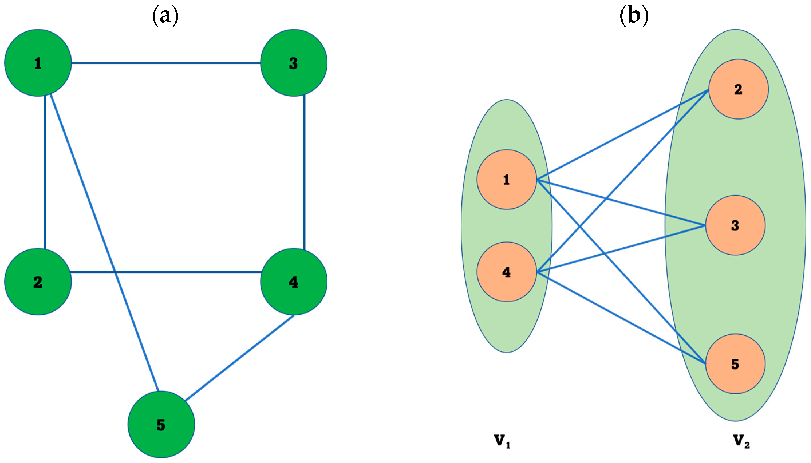
For example, the graph in Figure 1a represents 5 nodes labeled by numbers from 1 to 5. To check whether the given graph is bipartite, we need to apply the definition of a bipartite graph. In other words, we need to check if the nodes in the given graph can be partitioned into two disjoint sets, V1 and V2, with the abovementioned properties.
Figure 1b shows that the nodes or vertices of the graph shown in Figure 1a can be divided into two disjoint sets denoted by V1 and V2 in the figure. Furthermore, it can be seen that the nodes that are part of the set named V1 are not neighbors or adjacent to each other. However, each node in V1 is a neighbor or adjacent to nodes in V2.
To elaborate, in Figure 1b, node 1 and node 4 are members of V1. Form Figure 1a shows that these nodes are not neighbors. On the other hand, node 1, for example, is a neighbor of node 1, node 3, and node 5, which are members of the other set denoted by V2, as shown in Figure 1b.
As a result, it can be concluded that the graph shown in Figure 1 is bipartite because all the nodes or vertices of that graph are divided into two disjoint sets where the nodes in each set are not neighbors or adjacent. Still, at the same time, every node in one set is adjacent to nodes in the other set.
Thus, using a bipartite graph can improve the performance of the W.S.N. in two ways: (1). The mobile sink will visit smaller nodes, i.e., not all the nodes in the network in each round. (2). The proposed model will help stationary sensor nodes mix between multi-hop and single-hop communication, depending on which set is being visited and to which set the stationary sensor node belongs.
3. Mobility Models
Several research papers have suggested algorithms or models to support mobility in W.S.N.s. According to [22], the capacity of nodes in W.S.N.s to relocate themselves upon deployment is referred to as node mobility. As a result, there are two primary categories of sensor node mobility algorithms or models. The first is the usage of mobile sinks or sinks that can receive data from stationary sensor nodes while moving, whereas the second is based on providing all of the sensor nodes with the capacity to move. Because it is more pertinent to the proposed mobility model, we will focus our review in this paper on studies that supply a single mobile sink that moves to collect data from stationary sensor nodes and sends them to the base station.
The study proposed in [23] introduced a data-gathering method based on path planning to reduce distances traveled by the mobile sink and reduce the communication range. An inner center path planning algorithm was used to shorten the distance a mobile sink had to travel. The movement path back propagation problem was also considered by presenting a back-routing algorithm. Therefore, the proposed scheme must enable the mobile sink to make adaptive judgments to move adequately.
In addition, the research presented in [24] suggested addressing the relay selection problem to decrease energy use and increase the lifespan of W.S.N.s. As a result, the k-means method was used in the proposed study to partition the network into clusters. A movable sink-based cluster head selection technique was suggested to increase energy usage inside the cluster. The mobile sink node will function as a cluster head close to stationary sensor nodes to gather data and reduce energy consumption for static sensor nodes and the cluster head.
The research authors presented in [25] were written by writers who developed a sink mobility model derived from Korhonen’s self-organization map (S.O.M.). Their study establishes the mobile sink’s movement path using Korhonen S.O.M. The mobile sink thus moves during movement times and stops during pause periods. The mobile sink will remain in its present location during the stop periods for a fixed period, after which it will begin migrating to a new site determined using the Korhonen S.O.M., and so on, until topology changes brought on by energy depletion take place. As a result, a new Korhonen S.O.M. calculation of the mobility path will be performed.
To further improve the operation of environmental monitoring and anomaly search in W.S.N.s, a collaborative approach was presented in [26]. The proposed method is composed mostly of two components. Based on a weighted Gaussian coverage strategy, the first focus is collaboratively installing the static sensor nodes. The second section, on the other hand, focuses on path planning for the mobile sink and is based on modifying an active monitoring and anomaly search system that uses a Markov decision process model. The major objective is quickly identifying environmental irregularities so that the mobile mode can respond appropriately based on a cumulative reward function.
Another study that divides the network into zones to enhance wireless sensor network performance and extend their lifetime is proposed in [27]. The mobile sink will travel close to the heavily loaded zone. It is important to note that a fuzzy logic system is used to select the strongly loaded zone to address any uncertainties that may arise when making this choice.
Similarly, an adaptive mobile routing method concerned with identifying burst traffic is proposed in [28]. Additionally, the algorithm relies on splitting the network’s clusters into two groups, and the proposed network architecture is based on having two mobile sinks. After that, each sensor node will be in charge of one group and communicate with the cluster heads. Additionally, the mobile sink will visit the cluster heads within the group specifically. The mobile sink will, however, disregard the sequence in which the cluster heads are visited and move close to the heavily loaded cluster head if a traffic burst is detected.
An ant colony optimization-based end-to-end data-gathering technique was also presented in [29]. The proposed method is based on building a data forwarding tree and arbitrarily choosing data gathering points. As a result, the mobile sink’s route is estimated and described.
A sink mobility model using a genetic algorithms model is presented in [30]. The mobility model uses genetic algorithms to determine the direction the mobile sink should take when moving. After that, using single-hop routing, the mobile sink will travel to the nodes that are a part of the computed path to gather data from them via single-hop routing. On the other hand, multi-hop routing is used by nodes, not members of the mobile sink movement path, to forward packets to the mobile sink. Additionally, the portable sink’s movement is split into pause and movement periods to facilitate data communication and reduce changes in routing paths. To elaborate, the mobile sink migrates to new locations that are calculated using the proposed algorithm during the movement phase instead of the pause period, during which it remains in the current location.
Furthermore, a model based on creating mobile pathways for the mobile sink to decrease latency and energy usage was proposed in [31]. Choosing a meeting location, designing a trajectory, collecting data, and transmitting data are the four stages of the algorithm’s operation.
In [32], a mobile sink-based geographic routing scheme was developed. This study used two mobile sinks to gather information from sensor nodes in cells or geographic regions. As a result, each cell’s sensor nodes collect data and send it to the mobile sink. It is important to note that single-hop and multi-hop routing can connect sensor nodes to the mobile sink.
Consequently, several mobility models are presented in the literature. Some of these models are based on random mobility, while others try to use the current location of the mobile sink to calculate a new location. The work proposed in this paper approaches the problem of mobile sink path planning from a different perspective. The proposed approach aims to benefit from the network topology and the node neighborhood to create a logical topology based on bipartite graphs. After that, we use bipartite graph properties to derive a sink mobility model.
4. Proposed Mobility Model
The work proposed in this paper relies on randomly deployed W.S.N.s made up of N stationary sensor nodes and one additional node that can move to serve as a mobile sink node. Following network deployment, the base station receives the locations of the mobile sink and the stationary sensor nodes. Consequently, the base station calculates a bipartite graph, and the stationary sensor nodes are grouped into two disjoint sets, as explained in Section 2. It is worth noting that the mobile sink is not included in this calculation because it is supposed to visit stationary sensor nodes and collect information.
To clarify, a bipartite graph is derived by the base station using the locations of the static sensor nodes as a point of reference and the neighborhood data of the static sensor nodes. Thus, the stationary sensor nodes are grouped into two disjoint sets. The based station will also calculate the breadth-first traversal for the nodes in each subset based on the Euclidean distance between the static sensor nodes within each set. After that, based on the locations of the stationary sensor nodes, the mobile sink will choose one of the sets to start visiting stationary sensor nodes that are members of that set. In other words, the mobile sink will choose the nearest node to it and start visiting it; thus, it selects the set with the nearest member nodes to the mobile sink.
Consequently, the mobile sink will deal with the nodes in the selected set as a subgraph. The stationary sensor nodes within the set are visited according to the breadth-first traversal algorithm calculated based on the Euclidean distance between the nodes that are members of the selected set.
After visiting all the nodes in the first set, the mobile sink node will start moving towards the nearest member of the other set, and the static sensor nodes within that set will be visited according to the breadth-first algorithm that is calculated based on the Euclidean distance between the nodes that are a member of the new set. This process continues until a recalculation of the bipartite graph is triggered or required based on changes in the topology of the W.S.N. that might occur because of the death of static sensor nodes caused by energy depletion.
It is worth noting that when the mobile sink is visiting stationary sensor nodes in one set, it will be within the range of communication of other stationary sensor nodes that are members of the other set but are neighbors of the node being visited; thus, these neighbor nodes can send data to the mobile sink before being visited. Consequently, we can ensure that the nodes will not suffer from buffer overflow and that the sensed information will promptly be communicated to the mobile sink.
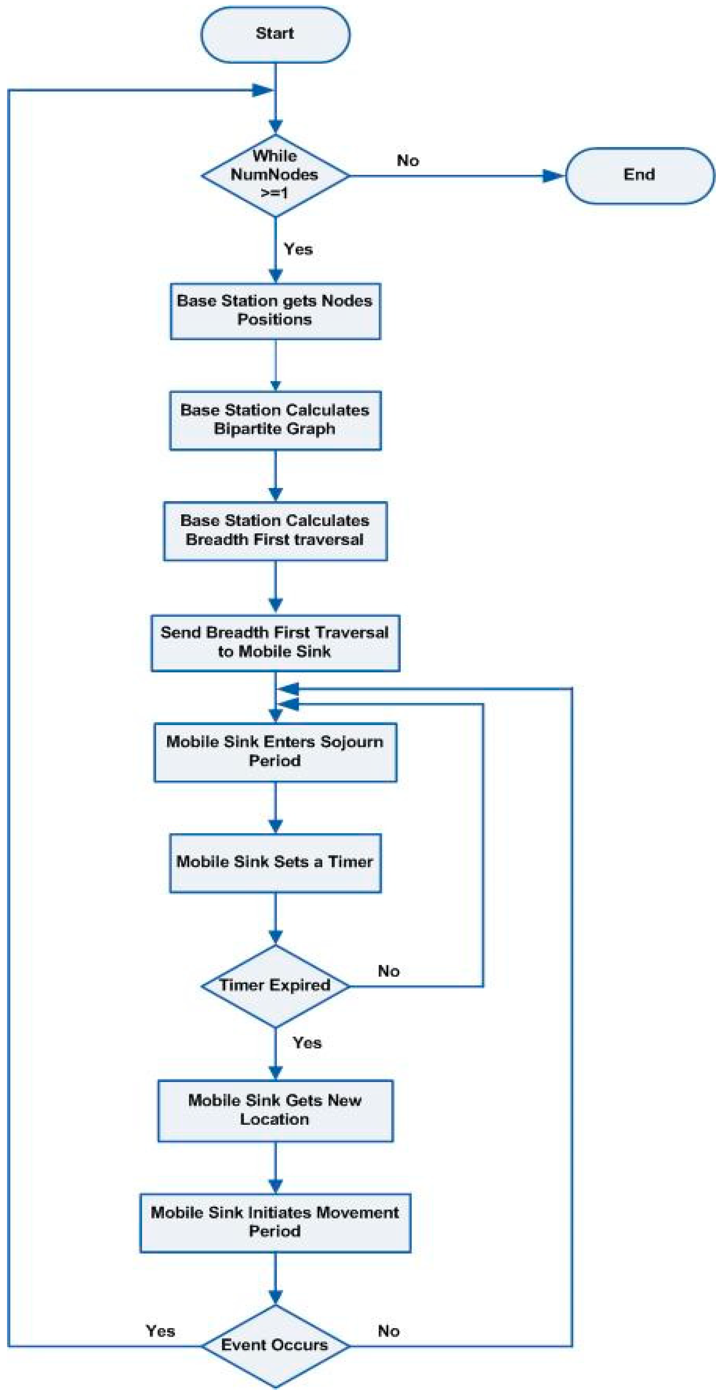
Furthermore, the mobile sink’s movement will follow the breadth traversal of the nodes in the selected set and is divided into sojourn periods and movement periods. In the sojourn period, the mobile sink will pause in its current location for a specific period. After that, it will begin moving toward a new location at a set pace. When the mobile sink arrives at the new location, the sojourn period begins again and stays in the new place for the same period. A flowchart of the mobility model suggested in this paper is shown in Figure 2.
Consider the networks shown in Figure 1a that were processed to deduce the bipartite graph in Figure 1b. Based on the Euclidian distance, the mobile sink will choose the nearest node to it to start its journey. For example, the mobile sink selected node 1, which belongs to V1, as the starting node of its journey. As a result, the mobile sink must visit all the nodes in V1 based on the breadth-first traversal algorithm. After visiting all the nodes in V1, the mobile sink will move to the nearest node in V2 and will visit all the nodes of V2 using the breadth-first traversal algorithm. Thus, the mobile sink will keep switching between the nodes of the two sets.
It is worth noting that when the mobile sink visits node 1 in V1, it will be a neighbor of some or all the nodes in V2. In this case, the mobile sink neighbors nodes 2, 3, and 5 from V2. As a result, data can be collected from the nodes being visited, their neighbors who are members of the other set, and so on. After pausing for a specified period at node 1, the mobile sink will move towards another node in V1, node 4. Thus, it will neighbor nodes 2, 3, and 5. Therefore, the mobile sink will be able to collect information from node 4 and its neighbors. Upon visiting all the nodes in V1, the mobile sink will move to the nearest node in V2. For example, the mobile sink will visit node 5 in V2, a neighbor to node one, and node four from V1. When the mobile sink arrives at the new location, i.e., near node 5, the mobile sink can collect information from node 5, node 1, and node 4 using single-hop communication.
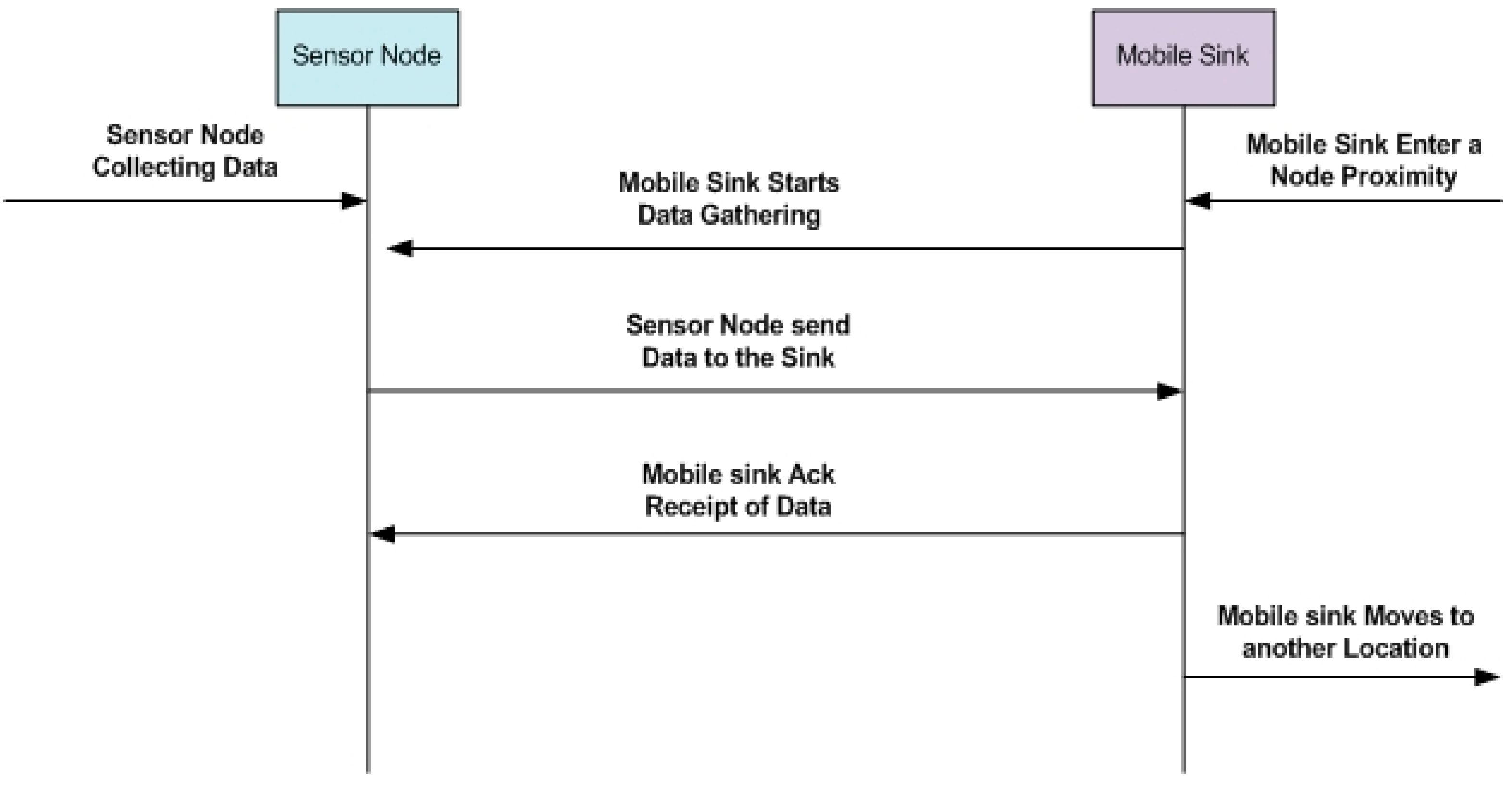
Consequently, by adopting this approach, the mobile sink will be able to visit nodes that are not neighbors to each other and collect data from the neighbors of the node being visited. It can also be observed that static sensor nodes will have multiple chances to report their data to the mobile sink, especially with multiple neighbors. As a result, up-to-date data will be collected from sensor nodes promptly. The chances of sensor nodes suffering from buffer overflow are reduced because static sensor nodes do not have to store the collected information for long, waiting to be visited by the mobile sink. Figure 3 shows a message flow diagram presenting the communication between the sink and the sensor nodes.
5. Simulation
5.1. Simulation Scenarios
Several simulation scenarios were run on the NS-2 simulator to examine the performance of the proposed sink mobility model. NS-2 is a discrete event-driven simulator designed to support research in communication networks. It supports wired and wireless networks and provides different protocols [33]. The Ad Hoc On-Demand Distance Vector (AODV) routing protocol conveys messages to their intended recipients. Static sensor nodes provide traffic at a steady bit rate (C.B.R.). AODV routing protocol was used because it is a reactive routing protocol. As a result, routing information to only some nodes are kept in the routing table constructed by AODV.
On the contrary, routing information will be obtained when needed to reduce the size of the routing table maintained by sensor nodes. Thus, processing time and memory consumed are reduced [17]. C.B.R. was also used to generate constant bit-rate traffic from stationary sensor nodes to study the proposed model’s performance under heavy-loaded conditions.
In addition, the effectiveness of the proposed mobility model was examined in networks consisting of 26, 51, 76, and 101 randomly distributed nodes in a grid of 1000 × 1000. Additionally, each network consists of N nodes numbered from 0 to n − 2 representing static sensor nodes for each network size. One additional energy-rich node serves as a mobility sink in the network, marked by . To further explain, the stationary sensor nodes in the network of 26 nodes are numbered from 0 to 24. A different node with the number 25 represents an energy-rich mobile sink node that will move between the stationary sensor nodes per the mobility model proposed in this work. Additionally, for each network size, the performance of the suggested model was examined for mobile sink speeds of 5, 10, 15, and 20 m/s. In Table 1, the simulation parameters are displayed.
5.2. Performance Metrics
The metrics used to analyze the network’s performance while utilizing the proposed mobility model include average end-to-end delay, packet delivery ratio, and throughput. The average end-to-end delay is the time a packet takes from its starting point to its ending point. By averaging the amount of time needed to send each packet between each source and each destination within the network, the average end-to-end delay for the entire network may be determined [34,35]. The average end-to-end delay is calculated using Equation (1):
In Equation (1), and represent the received transmitted copy of a packet, respectively, and N is the total number of received packets.
As stated in Equation (2), the ratio of successfully received packets to all packets transmitted is used to calculate the packet delivery rate [34,35,36]:
where Prs is the total number of successfully received packets, and present is the overall number of sent packets. The total number of correctly received packets throughout a certain period is the definition of throughput, and the third performance metric considered. As a result, in our simulation, throughput is computed as stated in Equation (3) by dividing the total number of packets successfully received by the total simulation time [34,35].
6. Simulation Results
This part shows and discusses the results of applying the simulation scenarios in Section 5.1. Each scenario was executed ten times to produce more detailed findings. The results of the 10 runs for each example were averaged to acquire the simulation results.
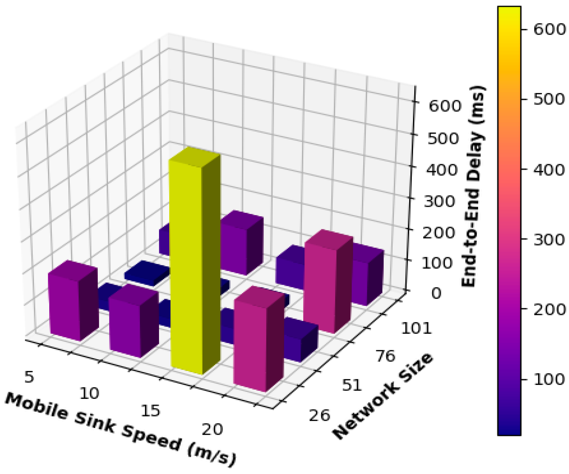
Figure 4 displays the average end-to-end delay results for various network sizes and mobile sink movement speeds. Networks with 51 and 76 nodes achieved the best overall results regarding the end-to-end delay, especially when the mobile sink speed was equal to 5, 10, and 15 m/s. The reason behind such behavior is that these speeds are considered low or moderate speeds of the mobile sink, which results in extensive multi-hop communication through long routes, which is the primary factor affecting the end-to-end delay results obtained for this case.
For other network sizes, it can be seen that the proposed mobility model obtained low and consistent end-to-end delay results, especially when increasing the speed of the mobile sink to be equal to 5, 10, and 15 m/s, which can be regarding the frequent use of single-hop communication because the mobile sink is moving at moderate speeds and visits static sensor nodes frequently. The network consisting of 26 nodes was an exception when the mobile sink speed was increased to 15 m/s. As is clear from Figure 4, the performance of this network increased dramatically because the network size is small and the speed of the mobile sink is relatively high, which may cause frequent changes and updates to the routing paths. Thus, multi-hop communication is used more frequently, and packets must go through extra and unnecessary hops to be delivered to the mobile sink.
On the other hand, when increasing the speed of the mobile sink to 20 m/s, these networks obtained higher end-to-end delay results because 20 m/s is considered a high speed and may cause frequent changes in the routing paths used to convey messages to the mobile sink. As a result, a packet may go through unnecessary hops to be delivered to the mobile sink.
For other network sizes, better results were obtained because the changes in the routing path did not affect all the nodes in the network. Hence, packets did not need to wander around or circulate through the network and go through some unnecessary and replicated intermediate nodes. Consequently, packets went through fewer hops until delivered to the mobile sink. As a result, smaller results for end-to-end delay were obtained.
Furthermore, Figure 4 shows that networks comprising 26 and 101 nodes obtained the worst performance compared to all other networks. This can be regarded as a result of the frequent use of multi-hop routing for the packets to be delivered to their destination. To put it in another way, the path to be adopted by the mobile sink is relatively short. As a result, the motion of the mobile sink will affect the routing paths for most of the static sensor nodes. Thus, packets sent from static sensor nodes will go through multiple hops, and some of these hops result from the changes or updates to the routing path. Therefore, those packets might have been routed more than once from the same node to adapt to changes in the routing path until they are delivered to the mobile sink.
Furthermore, Table 2 compares the results obtained for the average end-to-end delay for different network sizes and speeds of the mobile sink. It can be observed that medium-size networks, namely 51 and 76 node networks, performed better than other networks, especially when the mobile sink was moving according to low speed and moderate speeds equal to 5, 10, and 15 m/s. It can also be observed that the 51 nodes network obtained more consistent results than those obtained for 76 nodes for all speeds of the mobile sink. As a result, the mobility model proposed in this paper is more suitable for use with medium-sized networks when we aim to achieve low end-to-end delay.
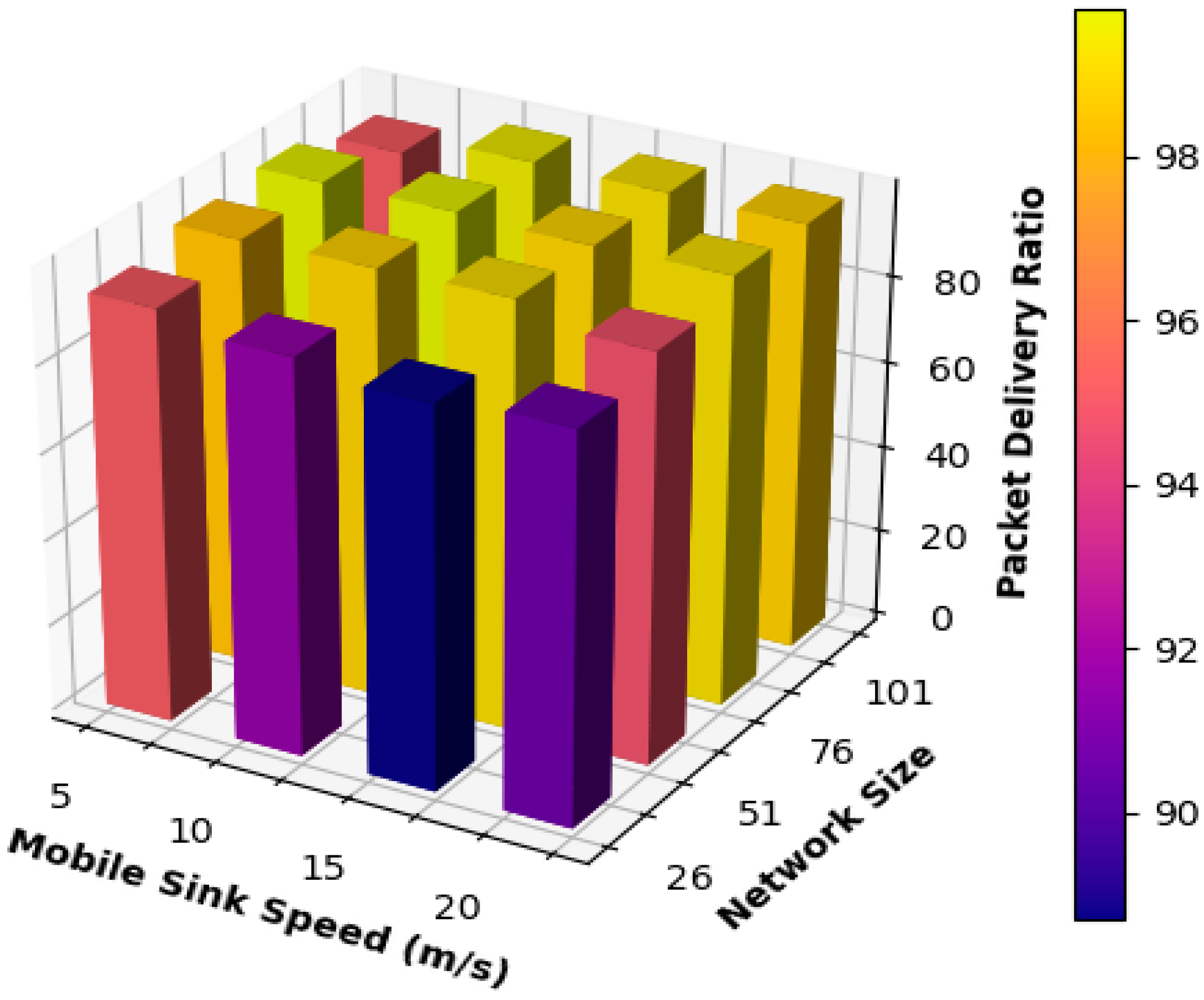
The results acquired for the packet delivery ratio are shown in Figure 5, which shows that the proposed mobility model obtained highly stable performance under all network sizes. The networks with 51 nodes and 76 nodes achieved the highest performance results regarding packet delivery ratio when the mobile sink speed was equal to 5, 10, and 15 m/s, consistent with the results from Figure 5.
To elaborate, since this network acquired the best results for the end-to-end delay, this will result in obtaining the highest results for packet delivery ratio due to the same reason discussed when explaining the results of Figure 1b. Additionally, from Figure 5, it can be observed that the increase in the velocity of the mobile sink to 20 m/s has affected the performance of all networks and caused a slight decrease in the performance of all networks. Thus, for small network sizes, when moving the mobile sink at high speed, frequent and rapid changes in the routing paths will take place and cause a decrease in performance. The mobile sink will also be moving at high speed, and completing data transmission between the mobile sink and the static sensor nodes will be challenging.
It can also be observed that the performance of the network consisting of 101 kept increasing when the speed of the mobile sink was increased because the higher the speed of the mobile sink, the more frequently the static sensor nodes are visited; thus, data can be transmitted to the mobile sink via single hop promptly, and static sensor nodes do not suffer from buffer overflow, which results from storing sensed information for long periods when waiting to be visited by the mobile sink.
On the other hand, for small network sizes, the mobile sink’s anticipated mobility path is smaller than that in medium- and large-sized networks. As a result, increasing the speed of the mobile sink to 20 m/s will affect static sensor nodes and their neighbors. Thus, these nodes will not have enough time to deliver packets to the mobile sink, and packets must be routed via multi-hop routing to be delivered to the destination. Packets will also go through unnecessary and extra hops to adapt to the frequent changes in the routing path to be delivered to the mobile sink.
Table 3 summarizes the result obtained for the packet delivery ratio and compares the results achieved by each network using different mobile sink speeds. The table shows that all networks achieved high-performance results in terms of packet delivery ratio, except the network consisting of 26 nodes. Table 3 shows that the 26 nodes’ network performance was lower than the performance of all other networks for all the different speeds used for the mobile sink. As a result, it can be concluded that all the speeds used for the mobile sink caused frequent updates to the routing paths. Thus, packets kept circulating in the network until they were dropped. This case was made even worse when the movement speed of the mobile sink was increased because the static sensor nodes did not have enough time to communicate with the mobile sink and deliver their packets using single-hop communication.
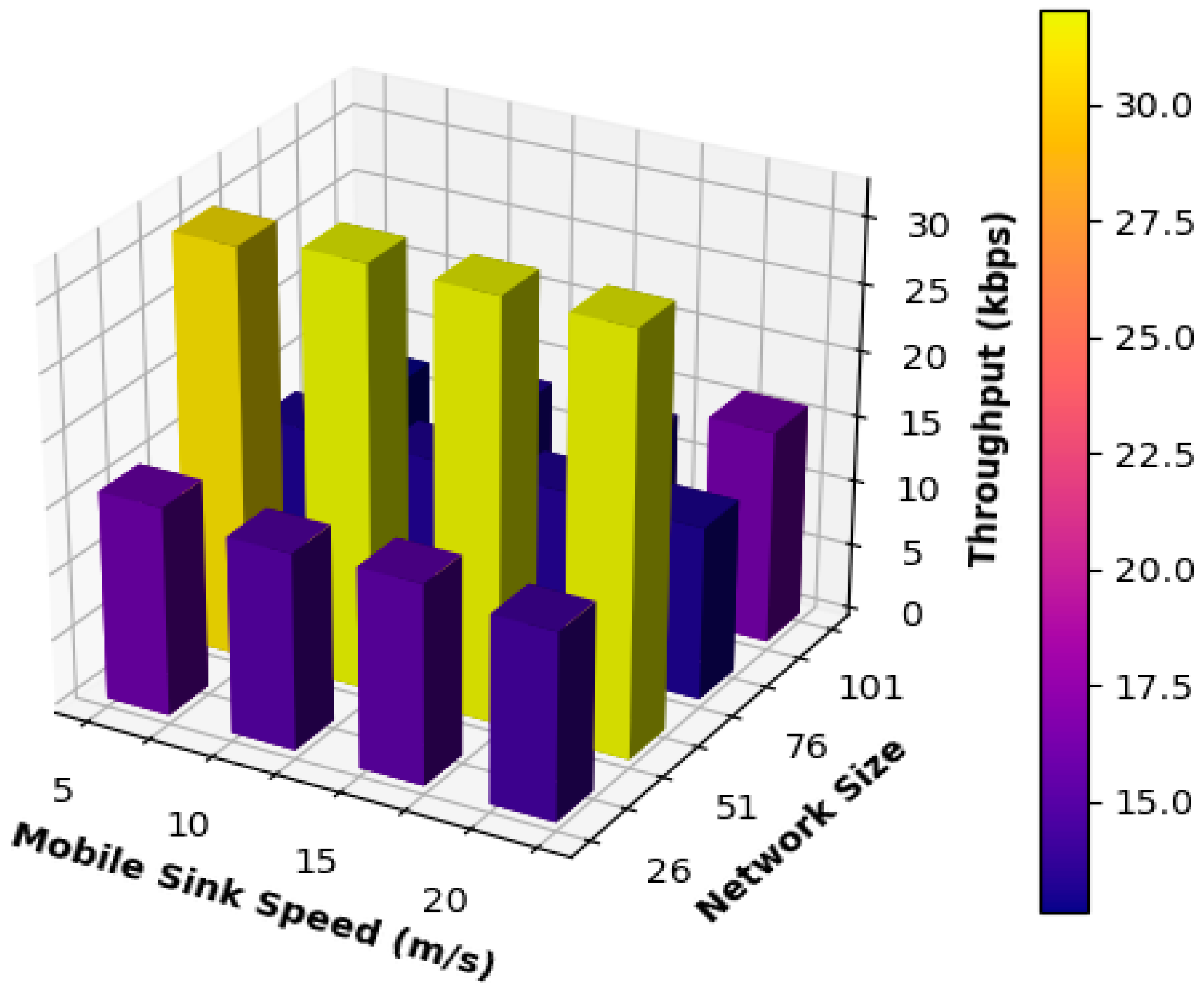
Figure 6 shows the results obtained for network throughput when the mobile sink moved following the suggested mobility model at various speeds and with varying network sizes.
From Figure 6, it can be seen that the proposed mobility obtained high and stable results for all network sizes under the speed of 10 and 15 m/s of the mobile sink because the mobile sink is moving at moderate speeds, which reduced the number of updates and the changes that may occur to the routing paths. Additionally, static sensor nodes will have a reasonable amount of time to communicate with the mobile sink and deliver data successfully. The performance of the network consisting of 51 nodes was the best and the most stable in all cases because the length of the routing paths was moderate; as a result, the packet did not have to go through many hops to be delivered. The length of the movement path adopted by the mobile sink was moderate; as a result, static sensor nodes did not need to update their routing tables frequently, and higher performance results were thus achieved.
For all other cases of mobile sink speeds, the performance of different network sizes was almost stable but was lower than that of 51 nodes’ networks. This was for one of two reasons. First, the mobile sink’s speed may not be suitable for the network size. To put it another way, high speeds may not be suitable for small networks, and low speeds may not be suitable for large networks because the network may be congested, and packets will be dropped. Second, for large network routing and low speeds, the routing paths may be very long, which might cause congestion in some parts of the network and result in a dropping packet. On the contrary, small networks operating under high speeds of the mobile sink packet may be dropped because of frequent changes in the topology and the routing paths, which results in consuming a large amount of the bandwidth to update the paths, which affects the network performance and increases the number of dropped packets.
Additionally, many packets may go through unnecessary hops to be delivered, and the time to live timer or the counter of the packet thereby expires, which results in the packets getting dropped.
Table 4 summarizes the results obtained for the network throughput and compares the results achieved by each network using different mobile sink speeds. From Table 4, it is clear that the network consisting of 51 nodes outperformed all other networks under all the different speeds used for the mobile sink. Consequently, for all other networks, using the different speeds of the mobile sink may have caused frequent updates to the routing paths, or the movement path adopted by the mobile sink was very long. As a result, static sensor nodes may have suffered from buffer overflow, and packets were dropped, affecting the performance of these networks.
7. Comparison with Other Mobility Models
Furthermore, the performance of the proposed model was compared to the performance of another three mobility models, namely, the Random Waypoint mobility model, the Gauss Markov mobility model, and the Depth First-based mobility model, using the same performance metrics. The simulation scenarios presented in Section 5.1 were executed on all models to obtain results and compare the models under the same circumstances. Table 5, Table 6 and Table 7 compare the performance of the four models. The three mobility models used in the comparison are discussed in Section 7.1, Section 7.2 and Section 7.3.
7.1. Random Waypoint Mobility Model
In this model, the motion of the mobile sink is divided into pause and movement rounds. Initially, the mobile sink will be in a pause round for a specific time. When the pause round expires, the movement round is initiated, and the mobile sink will randomly select a new location. It will start moving to that location at a specific speed. Upon arrival at the new location, a new pause round is started, and the mobile sink will stay in its location for a specified period, and so on [35,37].
This model was chosen for the comparison because its behavior is similar to the proposed model in this work. In other words, in both models, the movement of the mobile sink is divided into pause and movement rounds.
7.2. Gauss Markov Mobility Model
In order to create a more realistic model and to consider different randomness levels, this model was proposed. In this model, a mobile node has the ability to change its speed and direction when needed. At the initial stage, the mobile node is assigned a movement speed and direction, which will move according to these parameters for a specific time. After that, when the time expires, a new direction and speed are calculated based on the values used in the previous round [17,32]. This model was included in the comparison because it starts with assigned values for speed and direction. The new values are calculated from the previous rounds, similar to the proposed model. We start with one subset, and the new locations are selected based on the current location and the nearest neighbor.
7.3. Depth First-Based Mobility Model
The mobile sink will traverse the network in this model according to a graph’s Depth-First Traversal algorithm. As a result, the starting node is selected randomly, and the movement of the mobile sink is divided into pause periods and motion periods. After selecting the starting point, the mobile sink will move to the new location at a specific speed. It will stay there for a specific period when arriving at the new location. After that, the next location is calculated based on the Depth-First Traversal algorithm, and the mobile sink starts moving toward that location [38]. This model was selected because it has similar behavior to the proposed model in this work, as the motion of the mobile sink is divided into rounds, and the new location of the mobile sink is calculated based on a specified algorithm. It also uses the location of nodes and the properties on the topology or graph.
8. Conclusions
A sink mobility model that is built on creating a bipartite graph of the current network was presented in this paper. The proposed mobility model was then addressed after the concept of a bipartite graph was introduced. Additionally, the NS-2 simulator was adopted to run several scenarios to examine the performance and effectiveness of the mobility model presented in this research. Furthermore, the end-to-end delay, packet delivery ratio, and throughput were used to analyze the performance of the mobility model. Because the network with 51 nodes offered stable and respectable performance, the results demonstrate that the proposed mobility model performed better and is appropriate for use in medium-sized networks with moderate mobile sink speeds. Future research can build upon the work presented in this paper by measuring additional performance indicators, such as energy efficiency, routing overhead, and jitters. Furthermore, the suggested mobility model’s effectiveness can be investigated when employing routing protocols other than AODV. By examining these areas, researchers can gain a more comprehensive understanding of the system’s performance and potential limitations, thus paving the way for further improvements and innovations in this field. Moreover, comprehensive mathematical modeling and analysis can be conducted for other research problems in the same study area, thus contributing to a broader understanding of the proposed methods’ underlying mechanisms and potential applications.
Author Contributions
Conceptualization, A.A.T.; Methodology, A.A.T.; Software, A.A.T., Q.A.A.-H. and A.O.; Validation, A.A.T. and Q.A.A.-H.; Formal analysis, A.A.T. and Q.A.A.-H.; Investigation, A.A.T., Q.A.A.-H. and A.O.; Resources, A.A.T., Q.A.A.-H. and A.O.; Data curation, A.A.T.; Writing—original draft, A.A.T., Q.A.A.-H. and A.O.; Writing—review & editing, A.A.T., Q.A.A.-H. and A.O.; Visualization, A.A.T.; Funding acquisition, A.A.T., Q.A.A.-H. and A.O. All authors have read and agreed to the published version of the manuscript.
Funding
This research receives no external funding.
Data Availability Statement
No external data is associated with this research.
Conflicts of Interest
The authors declare no conflict of interest.
References
- Al-Rahayfeh, A.; Razaque, A.; Jararweh, Y.; Almiani, M. Location-Based Lattice Mobility Model for Wireless Sensor Networks. Sensors 2018, 18, 4096. [Google Scholar] [CrossRef] [PubMed]
- Segura-Garcia, J.; Calero, J.M.A.; Pastor-Aparicio, A.; Marco-Alaez, R.; Felici-Castell, S.; Wang, Q. 5G IoT system for real-time psychoacoustic soundscape monitoring in smart cities with dynamic computational offloading to the edge. IEEE Internet Things J. 2021, 8, 12467–12475. [Google Scholar] [CrossRef]
- Srinivasan, A.; Wu, J. TRACK: A Novel Connected Dominating Set based Sink Mobility Model for WSNs. In Proceedings of the 2008 Proceedings of 17th International Conference on Computer Communications and Networks, St. Thomas, VI, USA, 3–7 August 2008; pp. 1–8. [Google Scholar] [CrossRef]
- Sun, X.; Yang, Y.; Ma, M. Minimum connected dominating set algorithms for ad hoc sensor networks. Sensors 2019, 19, 1919. [Google Scholar] [CrossRef] [PubMed]
- Sikora, A.; Niewiadomska-Szynkiewicz, E. Mobility model for self-configuring mobile sensor network. In Proceedings of the Fifth International Conference on Sensor Technologies and Applications, SENSORCOMM, French Riviera, France, 21–27 August 2011; Volume 11, pp. 97–102. [Google Scholar]
- Sardouk, A.; Rahim-Amoud, R.; Merghem-Boulahia, L.; Gaiti, D. Data aggregation scheme for a multi-application WSN. In Proceedings of the IFIP/IEEE International Conference on Management of Multimedia Networks and Services, Venice, Italy, 26–27 October 2009; Springer: Berlin/Heidelberg, Germany; pp. 183–188. [Google Scholar]
- Razaque, A.; Elleithy, K.M. Energy-Efficient Boarder Node Medium Access Control Protocol for Wireless Sensor Networks. Sensors 2014, 14, 5074–5117. [Google Scholar] [CrossRef] [PubMed]
- Wang, P.; Akyildiz, I.F. Effects of different mobility models on traffic patterns in wireless sensor networks. In Proceedings of the Global Telecommunications Conference (GLOBECOM 2010), Miami, FL, USA, 6–10 December 2010; pp. 1–5. [Google Scholar]
- Yoon, J.; Liu, M.; Noble, B. Random waypoint considered harmful. In Proceedings of the INFOCOM 2003 Twenty-Second Annual Joint Conference of the IEEE Computer and Communications, San Francisco, CA, USA, 30 March–3 April 2003; pp. 1312–1321. [Google Scholar]
- Salvatore, J. Bipartite Graphs and Problem-Solving; The University of Chicago: Chicago, IL, USA, 2007. [Google Scholar]
- Navidi, W.; Camp, T. Stationary distributions for the random waypoint mobility model. IEEE Trans. Mob. Comput. 2004, 3, 99–108. [Google Scholar] [CrossRef]
- Garcia-Pineda, M.; Segura-Garcia, J.; Felici-Castell, S. A holistic modeling for QoE estimation in live video streaming applications over LTE Advanced technologies with Full and Non-Reference approaches. Comput. Commun. 2018, 117, 13–23. [Google Scholar] [CrossRef]
- Mbowe, J.E.; Oreku, G.S. Quality of Service in Wireless Sensor Networks. Wirel. Sens. Netw. 2014, 6, 19–26. [Google Scholar] [CrossRef]
- Premi, M.G.; Shaji, K. Impact of Mobility Models on M.M.S. Routing in Wireless Sensor Networks. Int. J. Comput. Appl. 2011, 22, 47–51. [Google Scholar]
- Jabour, F.C.; Giancoli, E.; Pedroza, A. Mobility support for wireless sensor networks. In Proceedings of the International Conference on Computer and Electrical Engineering, Phuket, Thailand, 6–10 July 2008; pp. 630–634. [Google Scholar]
- Camp, T.; Boleng, J.; Davies, V. A survey of mobility models for ad hoc network research. Wirel. Commun. Mob. Comput. 2002, 2, 483–502. [Google Scholar] [CrossRef]
- Taleb, A.A. A comparative study of mobility models for wireless sensor networks. J. Comput. Sci. 2018, 14, 1279–1292. [Google Scholar] [CrossRef]
- Aslam, S.; Farooq, F.; Sarwar, S. Power consumption in wireless sensor networks. In Proceedings of the 7th International Conference on Frontiers of Information Technology, Abbottabad, Pakistan, 16–18 December 2009; pp. 1–9. [Google Scholar]
- Al-Razgan, M.; Alfakih, T. Wireless Sensor Network Architecture Based on Mobile Edge Computing. Secur. Commun. Netw. 2022, 2022, 9073220. [Google Scholar] [CrossRef]
- Navarro-Camba, E.A.; Felici-Castell, S.; Segura-García, J.; García-Pineda, M.; Pérez-Solano, J.J. Feasibility of stochastic collaborative beamforming for long-range communications in wireless sensor networks. Electronics 2018, 7, 417. [Google Scholar] [CrossRef]
- Qureshi, K.N.; Bashir, M.U.; Lloret, J.; Leon, A. Optimized Cluster-Based Dynamic Energy-Aware Routing Protocol for Wireless Sensor Networks in Agriculture Precision. J. Sens. 2020, 2020, 9040395. [Google Scholar] [CrossRef]
- Jwair, Z.N.; Abdlhusein, M.A. Some dominating results of the topological graph. Int. J. Nonlinear Anal. Appl. 2022, 6, 1–9. [Google Scholar]
- Temene, N.; Sergiou, C.; Georgiou, C.; Vassiliou, V. A survey on mobility in wireless sensor networks. Ad Hoc Netw. 2022, 125, 102726. [Google Scholar] [CrossRef]
- Chang, J.-Y.; Jeng, J.-T.; Sheu, Y.-H.; Jian, Z.-J.; Chang, W.-Y. An efficient data collection path planning scheme for wireless sensor networks with mobile sinks. EURASIP J. Wirel. Commun. Netw. 2020, 2020, 1–23. [Google Scholar] [CrossRef]
- Taleb, A.A. Sink mobility model for wireless sensor networks using Kohonen self-organizing map. Int. J. Commun. Netw. Inf. Secure. 2021, 13, 62–67. [Google Scholar] [CrossRef]
- Guo, Y.; Xu, Z.; Saleh, J. Collaborative allocation and optimization of path planning for static and mobile sensors in hybrid sensor networks for environment monitoring and anomaly search. Sensors 2021, 21, 7867. [Google Scholar] [CrossRef]
- Prasanth, A.; Pavalarajan, S. Zone-based sink mobility in wireless sensor networks. Sens. Rev. 2019, 39, 874–880. [Google Scholar]
- Yalc, S.; Erdem, E. Performance analysis of burst traffic awareness-based mobile sink routing technique for wireless sensor networks. Gazi Univ. J. Sci. 2022, 35, 506–522. [Google Scholar]
- Wu, X.; Chen, Z.; Zhong, Y.; Zhu, H.; Zhang, P. End-to-end data collection strategy using the mobile sink in wireless sensor networks. Int. J. Distrib. Sens. Netw. 2022, 18, 1–12. [Google Scholar] [CrossRef]
- Taleb, A.A. Sink mobility model for wireless sensor networks using genetic algorithm. J. Theor. Appl. Inf. Technol. 2021, 99, 540–551. [Google Scholar]
- Alsaafin, A.; Khedr, A.M.; Al Aghbari, Z. Distributed trajectory design for data gathering using the mobile sink in wireless sensor networks. AEU-Int. J. Electron. Commun. 2018, 96, 1–12. [Google Scholar] [CrossRef]
- Naghibi, M.; Barati, H. Egrpm: Energy efficient geographic routing protocol based on the mobile sink in wireless sensor networks. Sustain. Comput. Inform. Syst. 2020, 25, 100377. [Google Scholar] [CrossRef]
- Network Simulator 2 (NS2): Features & Basic Architecture of NS2. Available online: https://www.tutorialsweb.com/ns2/NS2-1.htm (accessed on 21 April 2023).
- Taneja, S.; Kush, A. A survey of routing protocols in mobile ad hoc networks. Int. J. Innov. Manag. Technol. 2010, 1, 279–283. [Google Scholar]
- Amnai, M.; Fakhri, Y.; Abouchabaka, J. Impact of mobility on delay-throughput performance in multi-service mobile ad-hoc networks. Int. J. Commun. Netw. Syst. Sci. 2011, 4, 395. [Google Scholar] [CrossRef]
- Karyakarte, M.; Tavildar, A. Khanna, Effect of mobility models on the performance of mobile wireless sensor networks. Int. J. Comput. Netw. Wirel. Mob. Commun. 2013, 3, 137–148. [Google Scholar]
- Guezouli, L.; Barka, K.; Bouam, S.; Zidani, A. Implementation and optimization of rwp mobility model in W.S.N.s under tossing simulator. Int. J. Commun. Netw. Inf. Secure. 2017, 9, 1. [Google Scholar]
- Anas, A.T.; Tareq, A. Depth First Based Sink Mobility Model for Wireless Sensor Networks. Int. J. Electr. Electron. Comput. Syst. 2014, 19, 9–14. [Google Scholar]
Disclaimer/Publisher’s Note: The statements, opinions, and data contained in all publications are solely those of the individual author(s) and contributor(s) and not of MDPI and/or the editor(s). MDPI and/or the editor(s) disclaim responsibility for any injury to people or property resulting from any ideas, methods, instructions or products referred to in the content. |
Figure 1.
(a) A random graph, (b) Derived bipartite graph.

Figure 2.
A flowchart of the proposed model.

Figure 3.
Handshake diagram of the proposed model.

Figure 4.
Average end-to-end delay.

Figure 5.
Packet delivery ratio.

Figure 6.
Network throughput.


Table 1.
Simulation Parameters.
| Parameter | Value |
|---|---|
| Simulation Time | 500 s |
| Number of Nodes | 26, 51, 76, 101 |
| Pause Time | 5 s |
| Simulation Area | 1000 × 1000 |
| Traffic Type | C.B.R. |
| Mobile Sink Speed | 5, 10, 15, 20 m/s |
| Packet size (bytes) | 512 |
Table 2.
Average End-To-End Delay.
| Speed | Network Size | |||
|---|---|---|---|---|
| 26 Nodes | 51 Nodes | 76 Nodes | 101 Nodes | |
| 5 | 192.12 | 31.45 | 19.33 | 78.69 |
| 10 | 166.56 | 28.58 | 26.65 | 151.50 |
| 15 | 633.29 | 51.74 | 30.60 | 84.37 |
| 20 | 262.34 | 73.93 | 267.47 | 140.39 |
Table 3.
Packet Delivery Ratio.
| Speed | Network Size | |||
|---|---|---|---|---|
| 26 Nodes | 51 Nodes | 76 Nodes | 101 Nodes | |
| 5 | 95.20 | 98.52 | 99.81 | 95.25 |
| 10 | 91.63 | 98.96 | 99.81 | 99.57 |
| 15 | 88.70 | 99.24 | 99.02 | 99.25 |
| 20 | 90.63 | 94.83 | 99.25 | 98.88 |
Table 4.
Packet Delivery Ratio.
| Speed | Network Size | |||
|---|---|---|---|---|
| 26 Nodes | 51 Nodes | 76 Nodes | 101 Nodes | |
| 5 | 15.89 | 31.09 | 13.19 | 12.60 |
| 10 | 14.99 | 32.07 | 13.28 | 13.32 |
| 15 | 15.27 | 31.95 | 13.35 | 13.16 |
| 20 | 14.35 | 31.94 | 13.20 | 16.20 |
Table 5.
End-To-End Delay Performance Comparison.
| Model Name | Speed | Network Size | |||
|---|---|---|---|---|---|
| 26 Nodes | 51 Nodes | 76 Nodes | 101 Nodes | ||
| Proposed Model | 5 | 192.12 | 31.45 | 19.33 | 78.69 |
| 10 | 166.56 | 28.58 | 26.65 | 151.50 | |
| 15 | 633.29 | 51.74 | 30.60 | 84.37 | |
| 20 | 262.34 | 73.93 | 267.47 | 140.39 | |
| Random Waypoint Model | 5 | 1070.78 | 3590.09 | 5344.26 | 7348.23 |
| 10 | 1069.12 | 4247.96 | 4665.35 | 6904.05 | |
| 15 | 811.182 | 3507.06 | 5812.7 | 4860.76 | |
| 20 | 993.193 | 3535.66 | 6268.34 | 6077.27 | |
| Gauss Markov Model | 5 | 578.377 | 4642.27 | 6166.82 | 6084.23 |
| 10 | 231.716 | 3631.09 | 4142.33 | 7122.23 | |
| 15 | 461.982 | 2907.25 | 3492.46 | 4196.06 | |
| 20 | 579.801 | 3803.8 | 5322.32 | 6334.38 | |
| Depth First-Based Model | 5 | 153.439 | 2790.29 | 7334.31 | 12,043.8 |
| 10 | 116.511 | 3152.62 | 5937.32 | 11,173 | |
| 15 | 145.011 | 3335.92 | 6229.31 | 11,422.9 | |
| 20 | 392.171 | 3718.6 | 5352.08 | 11,506.4 | |
Table 6.
Packet Delivery Ratio.
| Model Name | Speed | Network Size | |||
|---|---|---|---|---|---|
| 26 Nodes | 51 Nodes | 76 Nodes | 101 Nodes | ||
| Proposed Model | 5 | 95.20 | 98.52 | 99.81 | 95.25 |
| 10 | 91.63 | 98.96 | 99.81 | 99.57 | |
| 15 | 88.70 | 99.24 | 99.02 | 99.25 | |
| 20 | 90.63 | 94.83 | 99.25 | 98.88 | |
| Random Waypoint Model | 5 | 59.76 | 34.80 | 20.76 | 14.84 |
| 10 | 53.55 | 31.82 | 19.16 | 13.32 | |
| 15 | 38.51 | 19.91 | 15.17 | 5.70 | |
| 20 | 39.72 | 26.49 | 13.85 | 9.47 | |
| Gauss Markov Model | 5 | 51.27 | 29.19 | 20.92 | 14.29 |
| 10 | 49.71 | 22.36 | 18.24 | 15.53 | |
| 15 | 35.44 | 22.18 | 15.42 | 11.47 | |
| 20 | 29.95 | 19.94 | 15.11 | 10.75 | |
| Depth First-Based Model | 5 | 55.91 | 37.62 | 19.38 | 9.06 |
| 10 | 56.92 | 34.54 | 19.93 | 10.64 | |
| 15 | 55.33 | 35.48 | 17.62 | 7.39 | |
| 20 | 53.08 | 33.62 | 18.34 | 7.19 | |
Table 7.
Throughput.
| Model Name | Speed | Network Size | |||
|---|---|---|---|---|---|
| 26 Nodes | 51 Nodes | 76 Nodes | 101 Nodes | ||
| Proposed Model | 5 | 15.89 | 31.09 | 13.19 | 12.60 |
| 10 | 14.99 | 32.07 | 13.28 | 13.32 | |
| 15 | 15.27 | 31.95 | 13.35 | 13.16 | |
| 20 | 14.35 | 31.94 | 13.20 | 16.20 | |
| Random Waypoint Model | 5 | 2.44 | 2.85 | 2.55 | 2.43 |
| 10 | 2.19 | 2.60 | 2.35 | 2.18 | |
| 15 | 1.57 | 1.62 | 1.86 | 1.18 | |
| 20 | 1.62 | 2.12 | 1.70 | 1.55 | |
| Gauss Markov Model | 5 | 2.09 | 2.39 | 2.56 | 2.34 |
| 10 | 2.03 | 1.83 | 2.24 | 2.54 | |
| 15 | 1.51 | 1.81 | 1.89 | 1.87 | |
| 20 | 1.22 | 1.63 | 1.85 | 1.76 | |
| Depth First-Based Model | 5 | 2.28 | 3.07 | 2.37 | 1.48 |
| 10 | 2.32 | 2.82 | 2.45 | 1.74 | |
| 15 | 2.27 | 2.90 | 2.16 | 1.21 | |
| 20 | 2.18 | 2.75 | 2.25 | 1.18 | |
Disclaimer/Publisher’s Note: The statements, opinions and data contained in all publications are solely those of the individual author(s) and contributor(s) and not of MDPI and/or the editor(s). MDPI and/or the editor(s) disclaim responsibility for any injury to people or property resulting from any ideas, methods, instructions or products referred to in the content. |
© 2023 by the authors. Licensee MDPI, Basel, Switzerland. This article is an open access article distributed under the terms and conditions of the Creative Commons Attribution (CC BY) license (https://creativecommons.org/licenses/by/4.0/).
Share and Cite
MDPI and ACS Style
Abu Taleb, A.; Abu Al-Haija, Q.; Odeh, A. Efficient Mobile Sink Routing in Wireless Sensor Networks Using Bipartite Graphs. Future Internet 2023, 15, 182. https://doi.org/10.3390/fi15050182
AMA Style
Abu Taleb A, Abu Al-Haija Q, Odeh A. Efficient Mobile Sink Routing in Wireless Sensor Networks Using Bipartite Graphs. Future Internet. 2023; 15(5):182. https://doi.org/10.3390/fi15050182
Chicago/Turabian StyleAbu Taleb, Anas, Qasem Abu Al-Haija, and Ammar Odeh. 2023. "Efficient Mobile Sink Routing in Wireless Sensor Networks Using Bipartite Graphs" Future Internet 15, no. 5: 182. https://doi.org/10.3390/fi15050182
Note that from the first issue of 2016, this journal uses article numbers instead of page numbers. See further details here.