1. Introduction
The high rate of patients not showing up for examinations and medical appointments is a recurring problem in health care. “No-show” refers to a non-attending patient who neither uses nor cancels their medical appointments. These patients’ behaviour is one of the main problems faced by health centres and has a significant impact on revenues, costs and the use of resources. Previous studies have looked at the economic consequences of a patient’s absenteeism [
1].
Each year, an average of about 30% of patients in the Brazilian state of Santa Catarina miss appointments, exams or scheduled surgeries. In 2018 alone, more than 52,000 patients did not attend scheduled procedures at health facilities in the state. This number represents 32.81% of the appointments given by regular centres. In absolute numbers, there were 52,710 patients who missed scheduled procedures in the first ten months of 2018, surpassing the figure for 2017, when 46,394 people failed to show up [
2].
Brazil has a universal health care system called SUS (Unified Health System). SUS is one of the largest public health systems in the world, and is the only one to guarantee comprehensive and completely free care for the entire population, including HIV patients, symptomatic or not, chronic kidney patients and cancer patients. The SUS Outpatient Network consists of 56,642 units, with an average of 350 million consultations being provided per year. This assistance extends from primary care to highly complex outpatient care.
In other Brazilian states the situation of medical no-shows is also present. In the city of Vitória, Espírito Santo, the number of absences from medical consultations in health centres reached 30% of the total appointments in 2014–2015. According to the City of Vitória, the average cost of an appointment during these years was approximately USD 37, which represented a loss of approximately USD 17.5 million for the government’s coffers [
3]. Given the impact that the non-use of health services causes in society, there is room for studies that present efficient solutions to this problem.
There is a general consensus in the literature that patient nonattendance is not random, and several studies have recognized the need to statistically analyse the factors that influence a patients’ no-show. Reducing the impact of missed appointments and improving health care operations are some benefits that this analysis may support. Some of the recent studies show that there is a relationship between the number of missed appointments and patients’ behaviour [
1,
4].
Furthermore, the work presented in [
5] carried out a study in the field of hospital radiology and grouped the extracted data into three groups: patient, examination and scheduling. The most informative aspects for predicting patients’ nonattendance for the exam were those based on the type of exam and the scheduling attributes, such as the waiting time between the appointment and the performance of the exam.
Long waiting lines, lack of resources to meet the demand and financial loss are consequences that the patient’s absence from the scheduled appointment can cause. To reduce these adverse effects, health centres have implemented various strategies, including sanctions and reminders [
6]. However, during the last decades, a sizeable number of medical scheduling systems have been developed to achieve better appointment allocation based on predictive models. Therefore, machine learning (ML) algorithms can serve as efficient tools to help understand the patient’s behaviour concerning their presence at a medical appointment.
A better understanding of the patient’s absenteeism phenomenon allows for the development of solutions to mitigate the occurrence of no-shows and contribute to the management and planning of health services. According to the context in which ML algorithms are applied, different observations are made, and new solutions can be modelled to mitigate absenteeism in medical appointments and exams. Thus, data collection and the application of ML algorithms in different contexts in healthcare should be explored, providing relevant information to assist in the decision process regarding the scheduling of appointments and exams.
There is currently one publicly available dataset present for patients’ no-shows which most researchers have been using. The open database is available on the Kaggle (
https://www.kaggle.com/joniarroba/noshowappointments, accessed on 25 November 2021) platform and refers to medical appointments scheduled in public hospitals in the city of Vitoria, in the state of Espírito Santo, Brazil. The downside of this dataset is the lack of information about how data was pre-processed and the huge class imbalance. Therefore, in our work, we have opted to collect the dataset on our own to obtain the most valuable information about the problem and help us to build more accurate classifiers.
To help understand the problem of absenteeism in medical appointments, we analyse the reasons that leverage the decision of a patient not to attend their medical consultation. Starting from the initial dataset, we identify the main factors related to the patient’s absence and propose a no-show classification model based on ML techniques. To compose the solution, algorithms that apply supervised ML techniques are used. As such, the present work brings to the current state-of-the-art a new contribution to elucidate the reasons for the no-show of healthcare patients.
The main contribution of the proposed solution is to build a predictive model that can serve as a baseline model for public health centres linked to the Brazilian universal healthcare system (SUS). Furthermore, this work demonstrated how machine learning techniques have real value in predicting a patients’ no-show and can help the public health sector in Brazil reduce costs and improve patient care and well-being. For that purpose, a new ML model is proposed and validated with real-life medical data, an essential tool for managing healthcare units.
The remainder of this paper is organized as follows. Section
1 presents an approach to the context of the research.
Section 4 describes the methodology applied in this study, including data analysis and the algorithms. Next,
Section 5 discusses the results. Finally,
Section 6 presents the final remarks.
2. Materials and Methods
Machine learning, as a subset of artificial intelligence, is a field of computer science that aims to develop algorithms that can improve through experience and by the use of incremental data [
7]. In the past decades, an increase in its research interest led to more and more areas of science finding application within ML algorithms. Application can be found in agriculture [
8], industry [
9], sensor networks [
10], fashion [
11,
12] or healthcare [
13,
14], just to mention a few examples.
When considering the healthcare environment, some studies apply ML algorithms to identify pre-eminent factors and characteristics of patients associated with the lack of attendance to the scheduled appointment [
1,
15,
16]. Other studies use statistical predictive models capable of predicting whether a patient will be absent from the appointment based on their historical data [
17]. Lee et al. [
18] described the development process up to the implementation of the predictive model in a real clinical environment, as well as the insights acquired using the model.
Despite the relevance of patient absenteeism in medical appointments, very few works use ML algorithms to identify and understand this problem. In this sense, ML was first applied in [
19,
20]. In these works, the publicly available dataset was used and guided the overall analysis. However, the lack of available attributes in the dataset did not allow the authors to build a solid predictive model. To the best of the authors’ knowledge, a study of the new private dataset with different attributes to analyse the data distinctly and validate new ML models for the no-show problem is still missing in the literature.
This work presents a statistical analysis to enumerate the potential reasons why patients do not attend appointments. In addition, we apply ML techniques to create models that better fit the absenteeism problem. As we are dealing with a dataset from a real-world environment, we began the data extraction and data analysis only after the research was approved and authorized by the Ethics Committee of the University of Vale do Itajaí. Thus, this work provides answers to some of the questions regarding patients’ non-attendance, that is:
- -
What are the key indicators that signal that a patient will not attend a scheduled appointment?
- -
What is the probability of a patient not showing up for an appointment?
2.1. Research Approach
The present work brings a new contribution to elucidate the reasons for the no-show of patients and build a ML model according to the following steps (see
Figure 1):
- 1.
Collect the patient dataset consisting of data from both appointments and patients;
- 2.
Apply data cleaning techniques to prepare the dataset;
- 3.
Include peripheral databases to add more value to the initial dataset;
- 4.
Analyse potential correlations between attributes in the dataset;
- 5.
Start a descriptive data analysis to detect key factors and trends that contribute to patients no-show;
- 6.
Adapt the dataset for the training and testing phase, and try several classification algorithms to process the data;
- 7.
Compare different performance metrics from the ML models, and select the model that provides the most accurate results for the problem at hand.
Figure 1 summarizes the building steps of the ML model, aggregating preprocessing, model building and model evaluation stages.
2.2. Data Preprocessing
2.2.1. Data Collection
The dataset used in this study consists of data obtained and extracted from the University of Vale do Itajaí Center of Specialization in Physical and Intellectual Rehabilitation (CER). The CER is an outpatient care service that performs diagnosis, assessment, guidance, early stimulation and specialized care. It has acted in functional rehabilitation and psychosocial qualification to encourage the autonomy and independence of people with disabilities [
21]. Firstly, we collected the relevant information–on the absenteeism problem–in loco at the rehabilitation centre by transcribing 4812 medical records from an electronic spreadsheet of 2017 and 2019. In the initial dataset, each file is composed of the following attributes:
- 1.
“Medical record number”: unique identifier of the patient’s record;
- 2.
“Gender”: male or female gender of the patient;
- 3.
“Appointment Date”: appointment date scheduled;
- 4.
“Attended”: given whether the patient attended the scheduled appointment or not;
- 5.
“No-show Reason”: description of the reason why the patient did not attend the scheduled appointment;
- 6.
“Type of Disability”: the patient’s motor or intellectual disability;
- 7.
“Date of Birth”: the patient’s date of birth;
- 8.
“Date of Entry into the Service”: date of the patient’s first appointment at the CER;
- 9.
“City”: city where the patient resides;
- 10.
“ICD”: identifier of the patient’s disease;
- 11.
“UBS”: basic health unit that sent the patient to be treated at the CER.
The dataset contains a target feature, identified by the variable “Attended” in which: “no” represents a patient that did not attend the medical appointment, and “yes” represents a patient that showed up. Unlike a system that performs a task by explicit programming, a ML system learns from data. It means that, over time, if the training process is repeated and conducted on relevant samples, the predictions will be more accurate.
2.2.2. Data Cleaning
This process converts (or maps) the data to another convenient format to carry out an analysis. In this work, the data manipulation process was performed in the virtual environment Google Colaboratory [
22], through the Python programming language [
23] with the help of libraries, such as pandas [
24] and NumPy [
25]. Firstly, we renamed the dataset columns. Secondly, we started the validation process. For the attribute “Attended”, we found that some values were in a different format than expected, such as “No”, “no”, and “Did not attend”. To deal with this inconsistency, we adjusted all values to the value “No” to standardize this attribute value—in this case, where the patient did not attend the scheduled appointment.
The expected value for the “Type of Disability” column was the letter “I” for intellectual disability and “F” for physical disability. However, we noticed that seven empty values, and three values outside the expected standard. In those cases, we amputated the empties values and corrected the others. Another validation of the data was related to the appointments date format. The initial data were not in the standard day/month/year. We provided the adjustment to this format. After this transformation, we considered only the data for 2019 and discarded the 90 medical records found for 2017.
2.2.3. Data Enrichment
In order to add more information to the collected data, some other databases were combined with the current database. Furthermore, new columns were created based on the existing ones. The following items describe this process.
Disease Data: As the initial database only contained the patient’s disease code, a new database with the names of related diseases was combined. With the inclusion of the disease names, data visualization and interpretation became more objective. The database with the International Classification of Diseases (ICD) was extracted from a file in PDF format on the government portal [
26], and transcribed to a file in JSON format. Initially, we adjusted the ICD registered in the database to the disease codes—extracted from the government portal—for the data merging. After the code standardization and data merging, we identified 37 diseases with different ICDs, and 1662 medical records without the registered disease code.
According to the graph in
Figure 2, we could check that some diseases stand out to the number of appointments.
Global Developmental Disorders,
Other General Symptoms and Signs, and
Child Autism together, corresponded to 66.31% of consultations carried out at the CER in 2019.
Weather Conditions Data: With the purpose of identifying whether weather conditions could influence patient absenteeism, we entered precipitation and temperature data into the dataset. We extracted the historical data with regard to the year 2019, from the National Institute of Meteorology (Inmet) [
27]. INMET’s database is feeding every 1 h and for each day presents 24 measurements of temperature and precipitation. Another relevant factor regarding the obtained data, the measurements are carried out only in the city of the meteorological centre. Since that Univali’s CER serves the region with eleven cities of AMFRI (Association of Cities of Foz do Rio Itajaí) [
28], only Itajaí has meteorological data from this data source. The measurement dates from the INMET dataset have converted to day/month/year format—they were in the US format, month/day/year—for data standardizing. Atmospheric pressure, speed and direction of the wind and air humidity data were discarded from the original dataset, keeping only the temperature and precipitation data. After data validation and standardization, the mean and maximum temperature and precipitation for each day were calculated and merged with the dataset of the medical records. The highest average temperature found was during April and November, remaining around 25 degrees. The temperatures registered were highest in April and October, approaching 34 degrees. Finally, a qualitative value has been assigned to represent the temperature and precipitation range. For temperatures, five classifications had considered: very cold, cold, mild, warm, and very warm. These classes represent temperatures less than or equal to 15 degrees, greater than 15 degrees, greater than 22 degrees, greater than 27 degrees and greater than 32 degrees, respectively. As for precipitation, we entered the following values: no rain, weak, moderate, strong, and very strong. This classification refers to the maximum precipitation of the day that has been less than 1 mm, greater than 1 mm, greater than 2.5 mm, greater than 10 mm and greater than 50 mm, respectively.
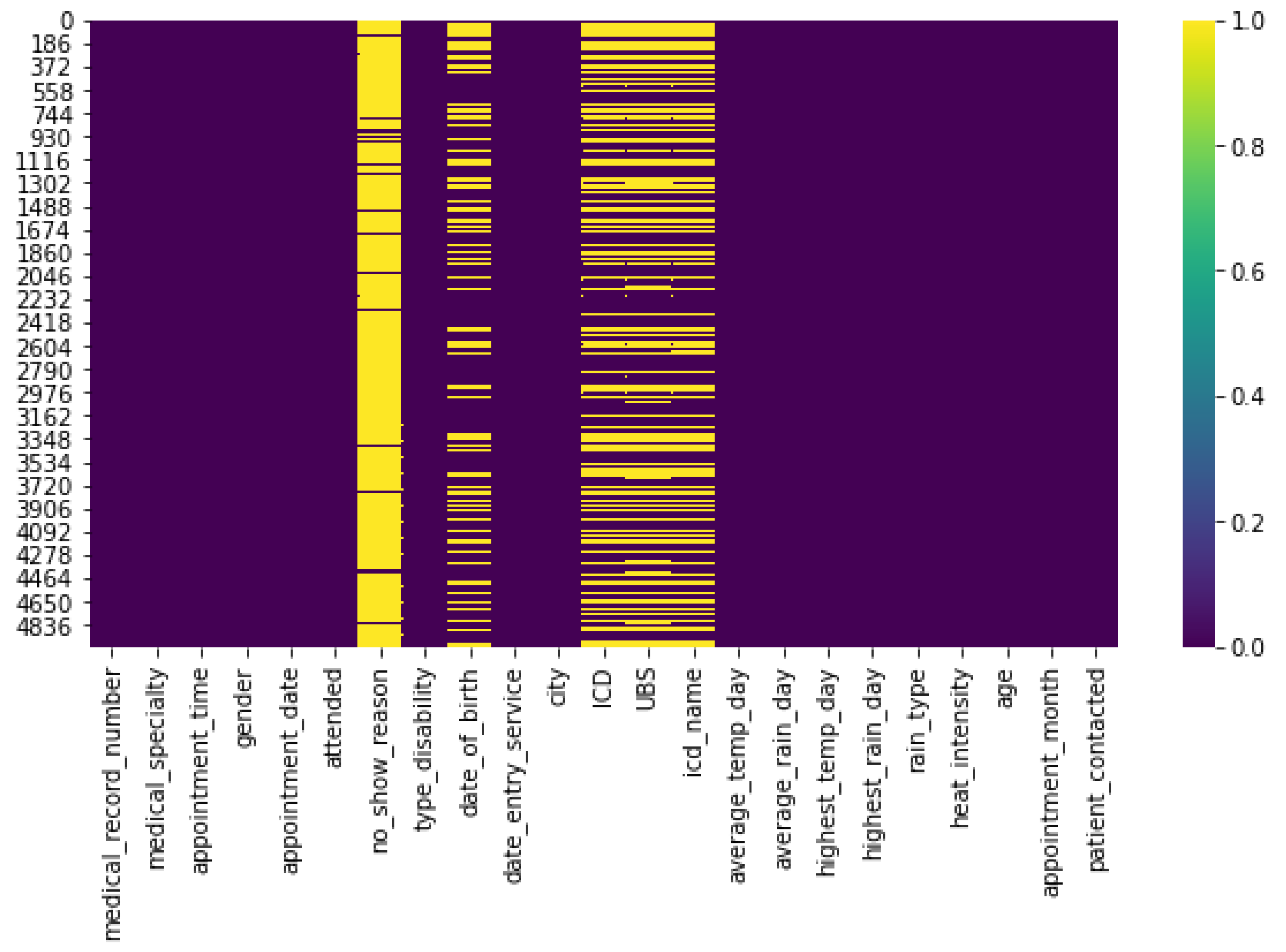
Other Related Attributes: We have created new attributes for the dataset based on the existing ones. From the date of birth included in the data, we derived the patients’ ages. In the same way, we extracted the month of the appointment from the date of the registration. Finally, we obtained the appointment shift based on the scheduled appointment time. The age attribute allowed us to analyse whether there is a relationship between the patient’s age and the rate of abstention from appointments. The month of consultation helped us identify a correlation with the level of abstentions being severity in the months in which there is a drop in temperatures. After achieving the validation process, merging new databases and inserting attributes in the original CER dataset, we kept 22 attributes to implement the initial data analysis.
Figure 3 presents the heat map of the attributes and their respective missing values: the dataset null value (in yellow) and the accurately filled value (in purple).
2.2.4. Data Exploration
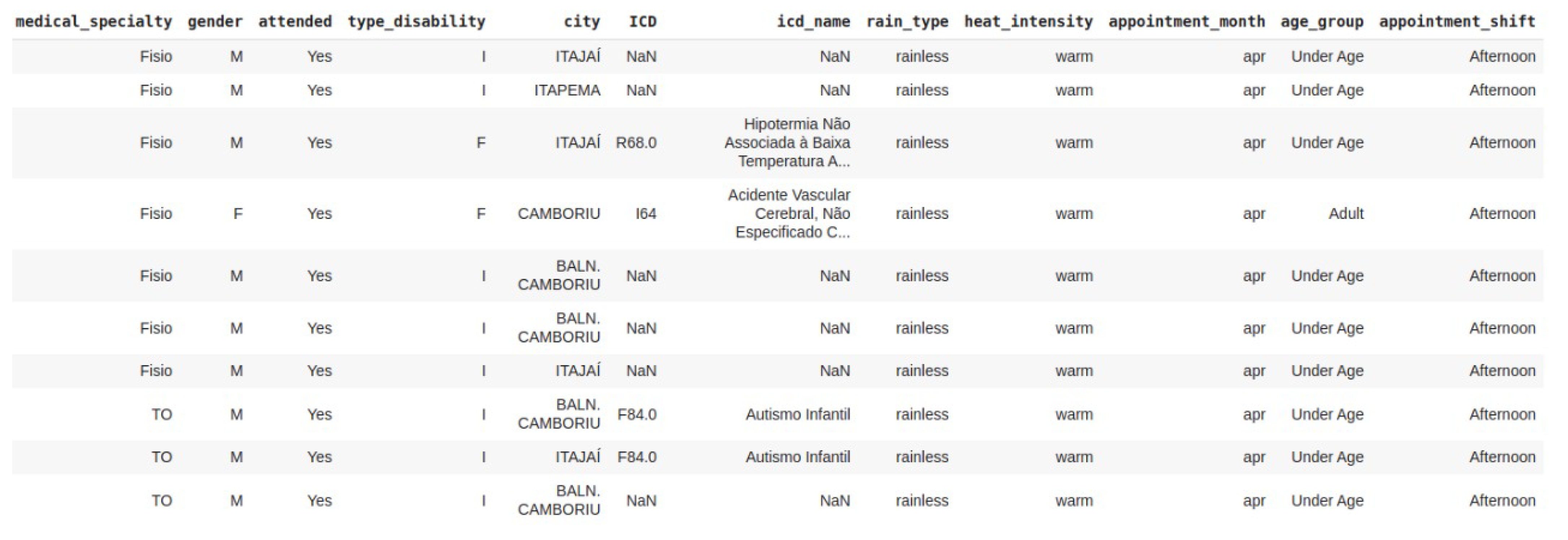
Data exploration is one of the steps responsible for exploring and visualizing data so that it is possible to identify patterns contained in the data sample. In this way, we enable inferences that can contribute to the understanding of the problem in question. One of the ways to summarize the data and obtain an overview of the attributes is through descriptive statistics. The use of descriptive statistics allows for summarizing the main characteristics of the dataset numerical characteristic (continuous or discrete), such as top, frequency, mean and standard deviation (std). However, in a scenario with a lot of categorical variables, other approaches may be more appropriate. An overview of categorical attributes is in
Figure 4.
Figure 5 presents the correlation matrix heat map. This figure illustrates the correlations between all variables: the gray fields do not represent any correlation, while the relative intensity of the yellow and blue colors represents an increase in correlation. In particular, it shows positive or direct correlation (in yellow)—in which the variation of one characteristic directly affects another—and negative or inverse correlation (in dark blue)—in which the fluctuation of one attribute inversely affects the other.
According to [
29], the correlation refers to the linear relationship between two numerical variables, usually denoted as x and y. Nevertheless, we recommended employing another statistical method because the available dataset has many categorical variables. Cramér’s V (also known as Cramér’s
) is one of the statistical correlation techniques developed to measure the strength of the association between two nominal variables [
30]. Unlike Pearson’s correlation, Cramér’s V assumes values in the interval
. The value 0 corresponds to the absence of association between variables, values close to zero correspond to a weak association, and values closer to 1 correspond to a stronger association.
Figure 5 presents the relationship of the numerical value using Pearson’s coefficient and categorical variables using Cramér’s V. By analysing the correlations in the heat map, we checked for attributes with high correlations. For both numerical and categorical attributes, a direct correlation is measured between 0.7 and 1 and, from −1 to −0.7 for inverse correlation in numerical attributes. However, the attributes related to the patient’s attendance at the appointment did not show a high correlation with any other attribute directly. The following features illustrate the correlations between the attributes of the dataset:
The age of the patient (“age”) and the ICD of the disease (“ICD”): patients in a certain age group are likely to have diseases caused by age;
Patient attending the appointment (“attended”) and the reason for not attending: the fact that the patient notified the reason for his/her non-attendance is directly related to the fact that he/she does not attend the scheduled appointment.
2.3. Descriptive Analysis
The descriptive analysis process begins with the observation of the distribution of the target variable within the dataset. This step was conducted by relating each feature to the target variable “attended”. In this section, we analyzed only the five most important characteristics.
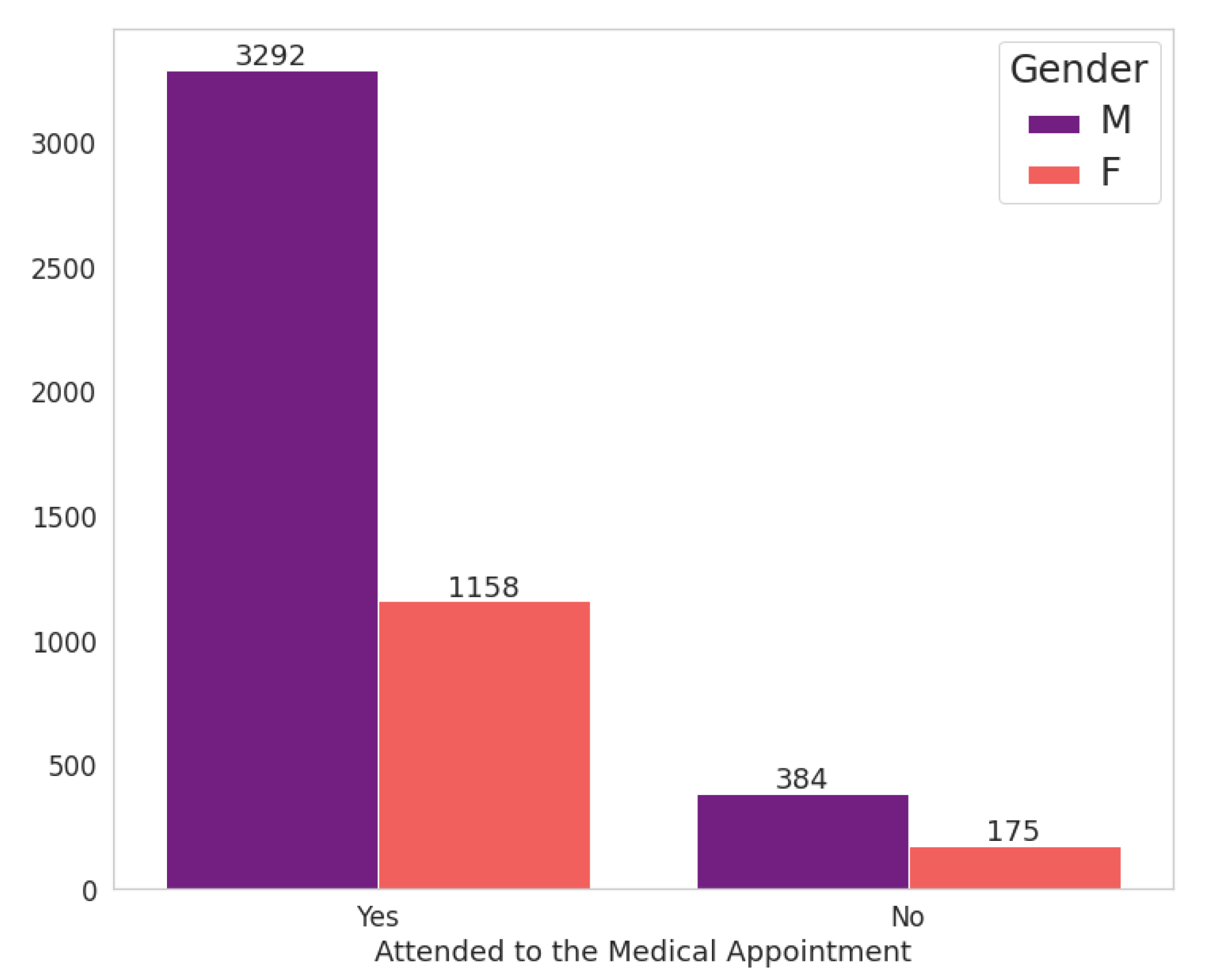
Figure 6 shows the relationship between the patient’s gender attribute and the fact that he (or she) attends the scheduled appointment. It should be noted that the proportion of consultations by women is much lower than that of men, 1333 and 3676 consultations for women and men, respectively. However, the amount of abstentions by women exceeds that of men, with female patients being responsible for 13.13% of abstentions against 10.45% for males.
Concerning the age of patients, we extracted two age categories for analysis: patients under 18 years old were labelled as “Minor Age” and the others as “Adult”. It is observed in
Figure 7 that there is an imbalance about these categories, with appointments for younger people being much more prevalent. Adults represent only 19% of consultations carried out at the specialized centre.
We also note that most of the data collected are from patients under 18 years old. It may reveal some characteristics of the behaviour of these patients that are not exclusively related to the patient who will receive care. In many cases, underage patients need someone close to accompany them in medical care. This fact implies a behavioural analysis of the patient and their companion. In this study, we did not collect data related to this issue.
We extracted the “appointment month” attribute from the existing column labelled “appointment date”.
Figure 8 shows that the month with the highest number of scheduled appointments is the month of September, followed by the months of October and August. In addition, the month with the fewest medical appointments is November. However, May, July and April are responsible for the highest abstentions from scheduled appointments. In May alone, the number of patients who scheduled medical appointments at the specialized centre and did not show up totalled more than 16% of the number of medical appointments.
As presented in
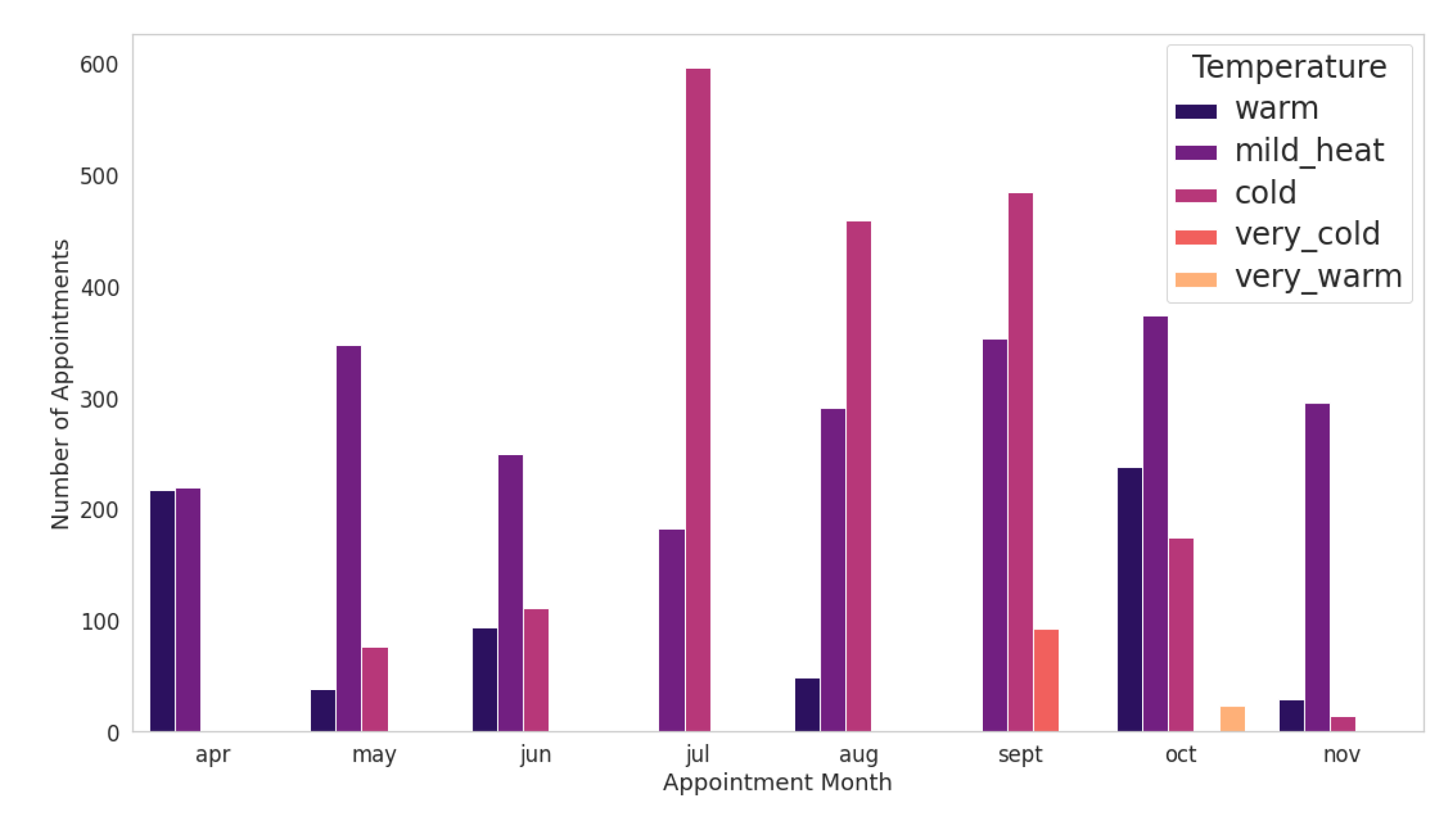
Section 2.2, we included climate data in the original dataset.
Figure 9 shows a way to visualize the relationship between weather conditions and the probability of the patient not attending the scheduled medical care. From
Figure 9, we observe that in autumn and winter, temperatures tend to be lower in the city of Itajaí, region of the medical centre.
In July, the number of patients who did not attend the scheduled appointment reached more than 15%. This fact may be related to the average temperature this month being the lowest in the year. However, based on
Figure 10, it is not possible to establish a direct relationship between the patient’s behaviour and their abstention from rain strength on the appointment day.
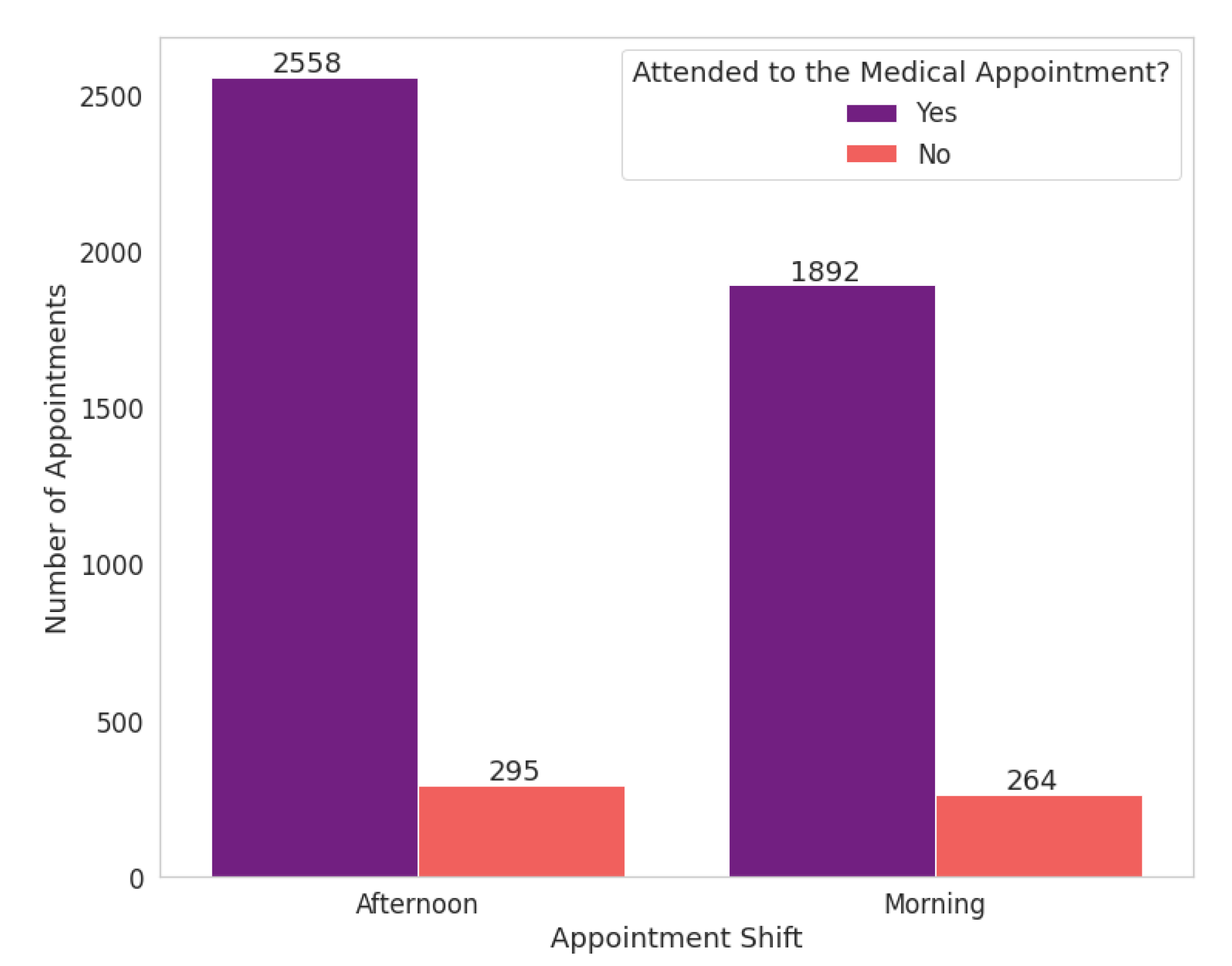
We extracted the appointment shifts based on the appointment time and divided them into “morning” and “afternoon” shifts. The morning shift refers to the period until midnight and the afternoon shift from this time on. Scheduled appointment times at the health centre range from 7 a.m. to 6:20 p.m. In the analyzed data, there are 35 different scheduled times; the time of 8:40 a.m. had the highest number of medical appointments.
The no-show proportion is similar for both shifts, in which 12.24% for the morning shift and 10.34% for the afternoon shift.
Figure 11 and
Figure 12 show that the absolute number of abstentions based on appointment times has low variability. When the highest frequency of scheduled medical appointments, the number of no-shows drops to around 9%, about 3% lower than the total number of abstentions for the morning.
In this way, although the hours most frequently present fewer abstentions, we can infer that the patients’ profile has not impacted the appointments during business hours. It is relevant to clarify that the focus diseases at the study’s medical centre mainly concern patients with motor disabilities. For this reason, possibly, they already have a routine with different hours.
3. Related Work
Logistic regression (LR) and Decision Trees (DTs) are the most commonly used techniques to predict missing attendance. Based on the literature review performed by [
31], Dervin et al. [
32] was the first author to use multiple LR to identify no-shows in 1978. They used ten predictors obtained from a small sample of 291 family practice centre patients but had disappointing results. They were only able to achieve an accuracy of 67.4% in a sample with an attendance rate of 73% [
31]. In contrast, the first work using DTs to identify no-shows was Dove and Schneider [
33] in 1981. The study analyzed whether the use of individual characteristics of the patient was better than considering the average rate of the clinic to predict missing appointments.
Many researchers have been exploring different techniques to improve the accuracy of predictive models in medical no-show contexts. The results confirm that the impact of understanding the patient’s behaviour related to his absence in a medical appointment has positive effects. Another aspect to note is that depending on the medical speciality, patients have different behaviours and should be accounted for when developing predictive models.
The authors of [
5] presented one approach focused on features specific to the radiology environment. Data from the radiology information system (RIS) was fused with patient income estimated from the United States census data. Logistic regression models were developed to predict no-show risk among scheduled radiology appointments in a hospital setting. After the validation process, the no-show prediction model yielded an AUC of 0.770. The cited work could strengthen radiology scheduling systems that do not have capability to predict no-show presence but have as main drawbacks its computational cost of train a predictive model in a large dataset and not validate the predictive model in other similar contexts.
In [
18], is presented a feature engineering approach to predict a patient’s risk of clinic no-show. The authors applied text mining techniques in order to extract useful information from the records collected. They build a no-show XGBoost model with the 15 top features and achieve an AUC of 0.793. Moreover, the authors describe the insights gained, and discuss modelling considerations on the trade-offs between model accuracy and complexity of deployment. Although the model developed in this work had good ability to identify clinic no-shows, it was based on a premise enterprise data warehouse that could be hardly adapted to other environments.
In the other three studies, the authors used the same public dataset to build their predictive models. The public dataset refers to medical appointments scheduled in public hospitals in the city of Vitória, in the state of Espírito Santo, Brazil. The authors of [
34] started from data cleaning and processing, exploratory analysis and finally had the highest accuracy on the test set with the Decision Tree algorithm. Similarly, in [
20] the authors explore the dataset following the same machine learning steps and obtained the same accuracy for both Decision Tree and Random Forest algorithms, 0.6 AUC ROC. Lastly, the work [
35] also built a solution based on the Decision Tree algorithm. However, a scheduling system was implemented such that the overall model detects whether a patient has a risk of missing an appointment with a 95% accuracy, upon which it automatically enables the risky patient’s schedule slot for overbooking and notifies medical staff or administration to contact them accordingly [
35]. Despite all these studies being based on a dataset from the public health system in Brazil, there is a lack of information in how this dataset was collected, pre-processed and even if its under any ethical and data confidentiality protocol.
Authors in [
36] develop a machine learning model for predicting no-shows in paediatric outpatient clinics. Three machine-learning algorithms (logistic regression, JRip, and Hoeffding tree) were compared and all models have precision and recall of around 90%. As a result, they found the most important features that impact the no-show rate in a paediatric clinic context: patient location, age group, nationality, appointment time, department, and clinic subspeciality. This work has some findings in its data explorations for underage patients in a paediatric clinic but lacks in exploring other than the traditional classifiers.
In [
37], a predictive model was developed to determine the risk-increasing and risk-mitigating factors associated with missing appointments. Then the model was used to assign a risk score to patients on an appointment basis across a range of medical specialities. Machine learning models were applied to different specialities and the performance varied by area: F1 score ranging from 0.4 to 0.61. Rheumatology is a speciality that there must be other factors that influence the no-show rates because only a 0.31 F1 score was reached. A key strength of this study is that it has included records from every medical speciality for an entire country, Wales. Nevertheless, only variables presented in the original dataset was considered and the influence of variables, such as weather or the impact of other events, were not taken into consideration for the predictive model.
The work presented in [
38] shows that the most important features in the prediction models developed were history of no-shows, appointment location and speciality. Information as age, day of the week, time of appointment, gender and nationality did not have a significant impact on the results. As a result, both JRip and Hoeffding Trees algorithms yielded a reasonable degree of accuracy. Then, this study shows that the higher the rate of a previous no-shows, the higher the chances that a patient will commit a no-show on subsequent visits.
A comparison was obtained between the model developed in this study and the related works considered. In
Table 1, we can see that the related works have distinct no-show rates, and the number of data from patients collected and data provenance vary significantly. These factors can influence the model’s accuracy in many ways. Different from the studies mentioned above that used a dataset from Brazil, this work collected an anonymized dataset from a public health centre, ensures the correctness of the samples and approved and authorized the usage of the data by the university Ethics Committee, to follow all restrictions of the General Data Protection Law. Related to performance measures, we can verify that none of the described works has the accuracy achieved in the model performed in this study. Moreover, this work is relevant as it provides a new look at the no-show problem in Brazil and can help restructure our public policies.
4. Model Building
In ML, classification problems are a form of supervised learning. These types of algorithms have multiple predictors and also a variable of interest responsible for guiding the analysis [
39]. On the other hand, unsupervised learning has only predictors (covariates) available and focuses on identifying patterns in data sets containing data points that are neither classified nor labelled.
In this study, the choice of algorithms was made based on the nature of the analyzed data and in the main goal to be achieved. As mentioned in
Section 3, LR and DTs are the most used algorithms to predict missing attendance, a binary classification problem. There are many other algorithms targeting classification problems, as support vector machines (SVMs) and Naive Bayes, but they are not suitable for this study based on this dataset characteristics. For example, SVMs are effective in high dimensional spaces and has as drawback not directly provide probability estimates, which implies in calculate using an expensive k-fold cross-validation. Then, the classification algorithms taken into consideration in this work are:
Logistic Regression classifier;
Decision tree classifier;
Random forest classifier.
This paper made use of the open-source scikit-learn (SKLearn) (
https://scikit-learn.org/stable/, accessed on 25 November 2021) library to develop supervised learning models. SKLearn library implements various ML algorithms and model performance analysis functions using the Python programming language. In the scope of this paper, we define a classification model as an algorithm implemented by a pre-defined function from the SKLearn library, which takes a distinct possible set of parameters.
Based on the overall steps presented in
Figure 13, the specific modeling steps for the proposed machine learning application are as follows:
- 1.
Collect and pre-process the data.
- 2.
Split data into a training set, and a testing set using holdout technique, described in
Section 4.2.
- 3.
Apply the three selected algorithms in the training set data to build a candidate model.
- 4.
Compute the candidate model score based on the testing set, to validate the model in unseen data.
- 5.
Check whether accuracy is greater than 90% in each trained model. If performance is less than 90%, then the proposed model is reevaluated, otherwise is picked as a candidate model.
4.1. Class Imbalance
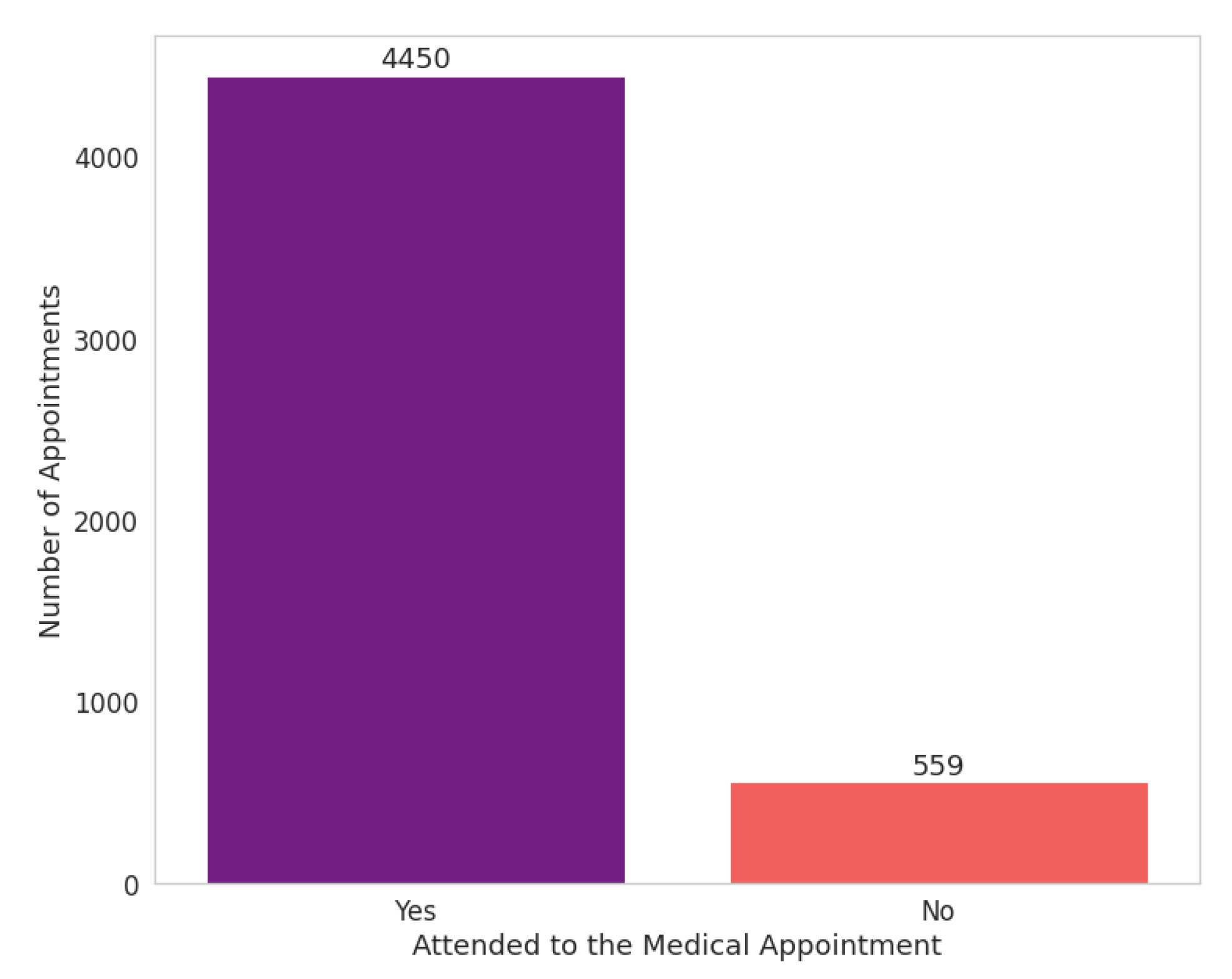
Upon inspecting the percentage distribution of the records between the “yes” (or “no”) attribute in the target variable “attended”, we find a considerable imbalance between both classes. An imbalanced classification problem is well-known, in which the distribution is biased.
Figure 14 shows 90% of the dataset’s records are labelled as “yes” and 10% are labelled as “no”.
Imbalanced classifications are a challenge for predictive modelling as most of the ML algorithms used for classification were designed based on the assumption of an equal number of examples for each class. This model generally results in poor predictive performance, specifically for the minority class. Thus, the problem is more sensitive to classification errors for the minority class than the majority class [
40].
To solve the problem of class imbalance, and after testing several different undersampling and oversampling algorithms, the Synthetic Minority Oversampling Technique (SMOTE) algorithm provided by the Imbalanced-learn (imblearn) (
https://imbalanced-learn.org/stable/references/generated/imblearn.over_sampling.SMOTE.html, accessed on 25 November 2021) library yielded the most considerable performance improvement. Not only did SMOTE solved the issue of class imbalance, but it also improved the classification performance metrics, mainly in precision and recall measures.
Figure 15 shows the target class after applying the oversampling algorithm.
4.2. Holdout and Cross Validation
The model must be trained on a consistent number of observations to refine its prediction ability to train the model to classify new patterns. If possible, two distinct datasets are the best choice: one for training and a second to be used as a test. In this case, as two dedicated datasets were not available, the original dataset was split in one part for training (70%) and another used for testing (30%), called the holdout method [
41].
The
train_test_split function, available in the SKLearn library, splits the data in both training and testing subsets. In the dataset split step, we need to keep the same distribution of target variables within both the training and test datasets. It is necessary to avoid that a random subdivision can change the proportion of the classes present in the training and test datasets from that in the original. Thus, even after the process of oversampling described in
Section 4.1, we apply the parameter “stratify” to the
train_test_split function to preserve the proportion of classes.
We applied the cross-validation technique to prevent overfitting problems and to estimate the performance of the model. According to [
42], in this technique, a dataset is randomly divided into
k disjoint folds of approximately equal size, and each fold is in turn used to test the model derived by a classification algorithm from the other
fold. Then, the performance of the classification algorithm is evaluated using the average of the
k accuracies resulting from the
k-fold cross-validation. There is no defined rule for choosing
k, although splitting the data into 5 or 10 parts is more common.
Figure 16 shows an overview of the cross-validation method.
5. Results and Discussion
This section presents the results obtained after performing the data pre-processing, adjusting the class imbalance using SMOTE oversampling, performing feature selection, and tuning algorithms hyperparameters per classifier. The results illustrate the performance obtained when testing the models mentioned in
Section 4 of this paper via multiple, defined metrics. To report on and evaluate model performance, we applied the following performance metrics [
44]:
- 1.
Accuracy: a simple ratio of total correct predictions over total wrong predictions.
- 2.
Precision (Positive predictive value): the ratio of correctly predicted instances per class to all predictions made for that same class.
- 3.
Recall (Sensitivity): the ratio of the correctly predicted instances per class to the total amount of actual instances labelled to that class.
- 4.
F1-score: a harmonic mean of recall and precision.
These results are acquired by drawing a confusion matrix for each classifier and then taking the average of the results. The confusion matrix enables visualization of the metrics, where the diagonal elements represent the number of points for which the predicted label is equal to the true label, while off-diagonal elements are those that are mislabelled by the classifier. After training all the three algorithms and fitting the Random Forest model with the test data, we obtained the confusion matrix shown in
Figure 17.
In the considered case study, we are interested in predicting the high number of patients who could not attend medical appointments by minimizing the incidence of false negatives. Thus, we selected the Random Forest classifier as the best classification algorithm able to achieve the objective of the analysis. In
Table 2, we summarize the classification report of the Random Forest model, which is related to precision, recall, and F1-score statistical metrics.
After the holdout process in the oversampled data described in
Section 4.2, we trained and tested the algorithm with 5963 and 2937 instances, respectively. The Random Forest algorithm correctly classified 2703 out of the total amount of test instances. Thus, the classifier obtained:
The highest true positive rate of approximately 92%, correctly predicting 1363 out of 1469 of the patients who do not attend the scheduled appointment;
The lowest false positive rate of approximately 0.07%. It only failed to detect 106 patients who had attended the appointment, obtaining the best recall score of 0.91.
The recall was identified as the most relevant performance metric to ensure the minimum number of false negatives (patients who may potentially attend the appointment but are not classified as such by the system) to a lack of precision resulted in considerable numbers of false positives. The Area Under the Curve (AUC) of Receiver Characteristic Operator (ROC) curve is an often-used performance metric for classification problems. It is one way to assess the rate of observed positives predicted as positives (sensitivity) and the proportion of observed negatives predicted as negatives (specificity). As closest to 1 the AUC is, better the model is at distinguishing between patients who will attend and not attend the appointment.
When developing a machine learning model, it is equally important not only have an accurate, but also an interpretable model. Often, apart from wanting to know what our model’s prediction is, we also wonder which features are most important in determining the result. By obtaining a better understanding of the model, it is possible not only verify it being correct but also work on improving the model by focusing only on the important features.
To evaluate the importance of features in a Random Forest model there are predominantly two methods: impurity and permutation feature importance. The main difference between them is that impurity-based feature importance can be misleading for high cardinality features (many unique values), whereas permutation feature importance overcomes this limitation. In contrast, the computation for full permutation importance is more costly. Besides that, as our dataset has not several features, we compute the importance of each feature in the Random Forest model employing permutation importance technique. The results can be shown in
Figure 18 and
Figure 19.
The attributes that most influence the model’s prediction are the appointment’s month (especially September, July and August) and whether or not the patient was contacted before the appointment. This can reinforce the previous data analysis that indicated that in rainy or cooler days patients tend to miss their medical appointments. On the other hand, when the patient is encouraged to confirm their scheduled appointment few days before by a contact from the health centre, their chance to miss their appointment falls drastically. However, despite the importance of these features, even after removing the other features from the dataset and generating a new model with the same algorithm with the most relevant attributes, the models had the same performance.
A key strength of this study is to elucidate a new way to reduce costs and improve patient care in Brazilian health care system. Without the SUS, the 78% of the population that does not have private insurance would not have had proper access to health services. In a large health system as in Brazil, the impact of solutions that use machine learning to improve the access to the services is huge. While most studies focus on the private health system, this study has included records from the public health care system in Brazil. Besides that, the dataset analyzed was restricted mainly to patients with motor disabilities and underage patients. Solutions involving treatment of patient data privacy should also be considered, as described in [
45,
46]. This can be challenging because is a sample with very specific characteristics and maybe could not be properly generalized to other health specialities. Although, as a starting point for validation of predictive models for medical no-show problem, this work can be valuable.
6. Conclusions
This study aimed to build a no-show classification model for patients and investigate the meaningful features that signal that a patient will not attend the scheduled medical appointment. To achieve the results, we applied some ML techniques to identify the factors that may contribute to the absenteeism of the patients and, above all, to predict the likelihood of individual patients not attending the scheduled appointments.
After analyse the performance metrics, the Random Forest model seemed to be a good choice to be the final model for the available dataset. It revealed the best recall rate (0.91) and achieved an overall false-negative rate equal to 0.08% of the total observations. The proposed predictor and analysis results demonstrate that the attributes that can influence the patient’s attendance in a medical consultation are the lower weather temperature and the appointment time. However, many other factors may implicitly influence the patient’s no-show that could not be inferred from the analyzed dataset.
The results obtained from the data analysis represent a starting point in the development of efficient patient no-show classifiers in Brazil. In particular, this work can help the improvement of solutions to the public health system with the help of machine learning techniques. For future studies, we are in the process of collecting a larger dataset that includes records from every medical appointment made by the public health system in southern Brazil. The availability of additional information on patients and medical appointments may help to improve the ability of the model to learn new behaviours.


 ,
, 


