
Quantitative Assessment of Forest–Tundra Patch Dynamics in Polar Urals Due to Modern Climate Change


1
Institute of Physics and Technology, Ural Federal University, 19 Mira Street, 620002 Yekaterinburg, Russia
2
Institute of Forest and Natural Resource Management, Ural State Forest Engineering University, Sibirskiy Trakt, 37, 620100 Yekaterinburg, Russia
3
Institute of Natural Sciences and Mathematics, Ural Federal University, 19 Mira Street, 620002 Yekaterinburg, Russia
*
Author to whom correspondence should be addressed.
Forests 2023, 14(12), 2340; https://doi.org/10.3390/f14122340
Submission received: 9 October 2023
/
Revised: 22 November 2023
/
Accepted: 23 November 2023
/
Published: 29 November 2023
(This article belongs to the Special Issue Forest Coverage and Spatial Distribution of Tree Species under Regional and Global Changes)
Abstract
:The spatial and temporal dynamics of the Siberian larch (Larix sibirica Ledeb.) at the upper limit of its growth on the south-eastern macroslope of the Rai-Iz massif (Polar Urals, Russia) during the second half of the 20th to the beginning of the 21st century were analyzed. Current climate changes were accompanied by increased stand density on previously wooded parts of the mountain slopes and the appearance of new forest generations in lightly wooded or unforested parts of the studied area. Our original method for the automated recognition of boundaries among the key phytocoenohoras (closed forest, open forest, light forest, and tundra with single trees) is universally applicable and improves objectivity in selecting boundaries for these phytocoenohora types. With regard to the total area of the study site, the area of closed forest, open forest, and light forest, respectively, increased from 2.9% to 6.8%, from 9.6% to 13.1%, and from 7.5% to 15.6%, while the area of tundra lots with single trees decreased from 79.9% to 64.5%. Phytocoenohora type replacement in the course of the study period was characterized by a transition from forms with lower density to higher-density forms. Changes in the opposite direction were not discovered. Natural wind protection barriers for young larch tree generations included hummocks and groups of grown trees. The process of gradual tundra and forest tundra forestation then began on the leeward side of the barrier close to seed-producing trees.
1. Introduction
Vegetation at the upper and northern limits of its habitat is a sensitive indicator of climate condition changes; therefore, multiple researchers use mountainous and northern territories as monitoring sites to assess early biota responses to climate change [1,2,3,4,5,6,7]. One of the indicators for changes occurring in wooded tundra biocoenoses is the quantitative assessment of the value and speed of horizontal and vertical vegetation boundary shifts [8,9,10,11,12].
The complexity of assessing climatogenic changes that occur in forest and forest tundra biocenoses near the upper treeline based upon the changes in the spatial distribution of the trees is determined by several causes. These include methodological problems with selecting vegetation cover boundaries, as the cover simultaneously possesses discretion and continuity properties. The appearance of sharp boundaries is a special case of the ecotone concept and, as a rule, is due to contrasting environmental conditions. Natural boundaries are rarely sharp and, in general, human-related boundaries are sharper then natural ones [13]. Besides this, every transitional zone represented by a polygonal object can be reduced to a boundary, i.e., a linear object, if the said simplification allows one to penetrate deeper into the essence of the researched phenomena. Differences in terminology and the implied meanings of terms cause misunderstanding among researchers and can become a problem while comparing results obtained by different authors. For example, it is often impossible to perform quantitative comparisons for different regions when using treeline spatial position changes as an indicator of tree vegetation response to climate change due to the fact that publications do not specify the meaning of treeline implied by the authors [14]. At the same time, some researchers consider that the “treeline” term is intuitively clear and does not require additional explanation. Jobbagy and Jackson [15] were forced to exclude publications without clear definitions while comparing data on forest boundaries from different sources. This approach was substantiated by differences in both the characteristics and their critical (threshold) values required to draw boundaries and the understanding of what constitutes a boundary itself.
The “upper treeline” can represent an ecotone extending from the dense forest boundary to the physiological limit of tree growth [14,16], one of the transitional-zone boundaries [17], or a line that is located in the intermediary position between the upper boundary of a dense forest and an upper boundary of tree species growth [18].
It is possible to specify two families of methods used to solve the problem of boundary recognition: clustering algorithms designed to form groups (areas) that are uniform with regard to a selected criterion, and boundary recognition methods that define change areas of vegetation cover parameters that are important in the opinion of the researcher [19]. The method used in this work can be assigned to the first of the above method families.
In the case of using clustering methods, boundaries are formed as a by-product among the selected areas belonging to different spatial clusters. The implementation of methods for selecting change areas may include the analysis of the first or second partial derivatives of the measured variables by the spatial coordinates [20]. A substantial portion of boundary recognition algorithms were developed and are used for digital image analysis [21,22].
The representation of an upper treeline as a solid line often requires a certain level of generalization, partially due to isolated clumps of trees separate from the main forest massif. Therefore, for this type of boundary representation, improved visibility lowers the precision of the shift size quantitative assessment.
The purpose of this study was twofold: (1) to demonstrate an effective method for mapping and analyzing woody vegetation cover change close to the upper limit of growth and (2) to highlight the climate-driven changes occurring in the upper treeline ecotone of the study area in the Polar Urals over a time interval of more than fifty years.
2. Materials and Methods
2.1. Study Area
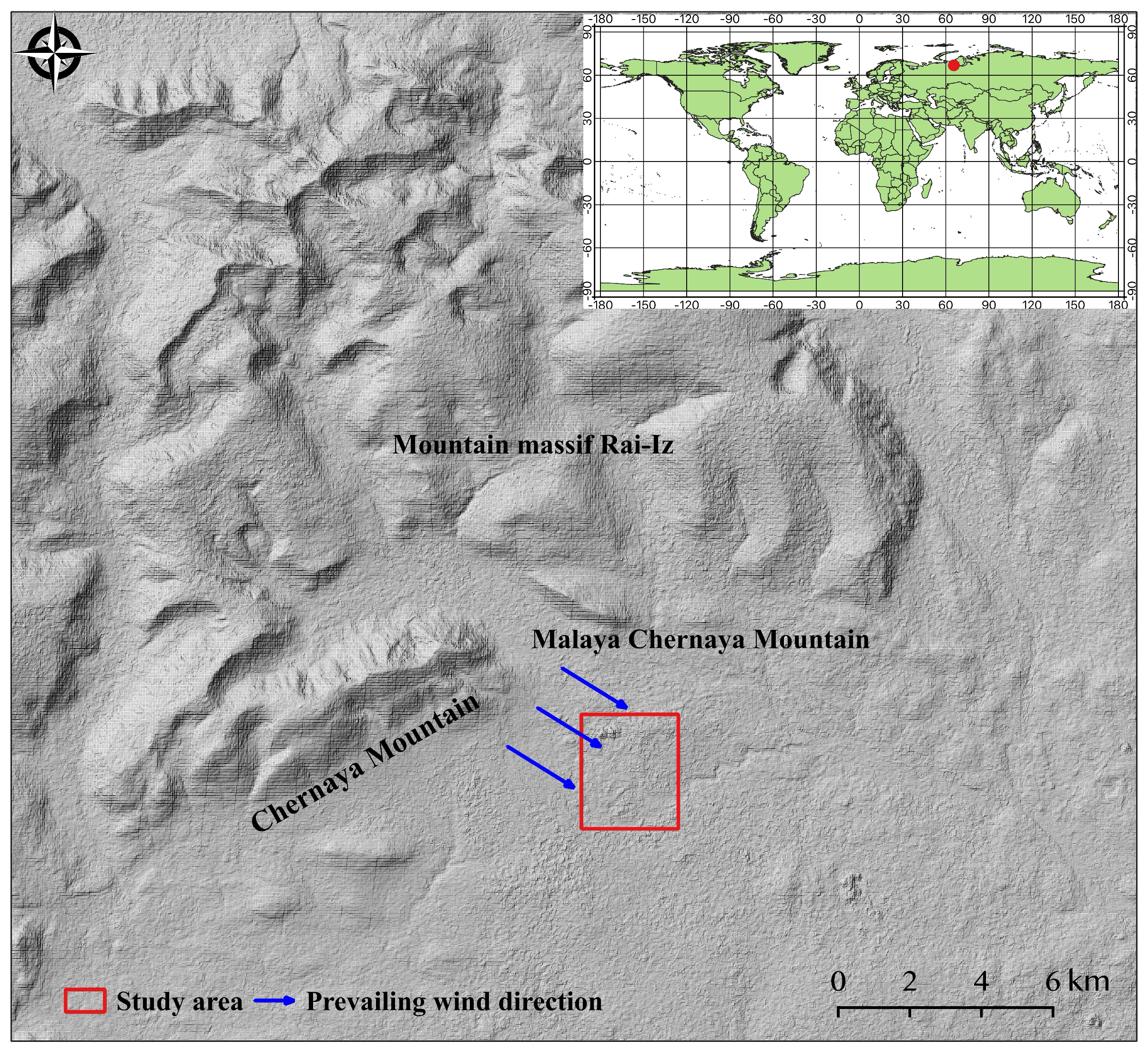
The study area (66°3028–66°4742 N, 65°4928–65°3359 E) was located on the southeastern slope of the Pai-Iz massif (Polar Urals, Russia). The surface of the area was formed by a glacier in the course of the last global glaciation, which ended about 10 Kya [23]. From the west, the area is limited by the Yengaiu river, the right bank of which in this area was formed by a right lateral moraine. The eastern boundary of the site follows the left lateral moraine. Glaciation caused a large number of ridges, knolls, and depressions within the study area. The upper part of a glacier was located on the Rai-Iz massif (Figure 1), which is composed of peridotites.
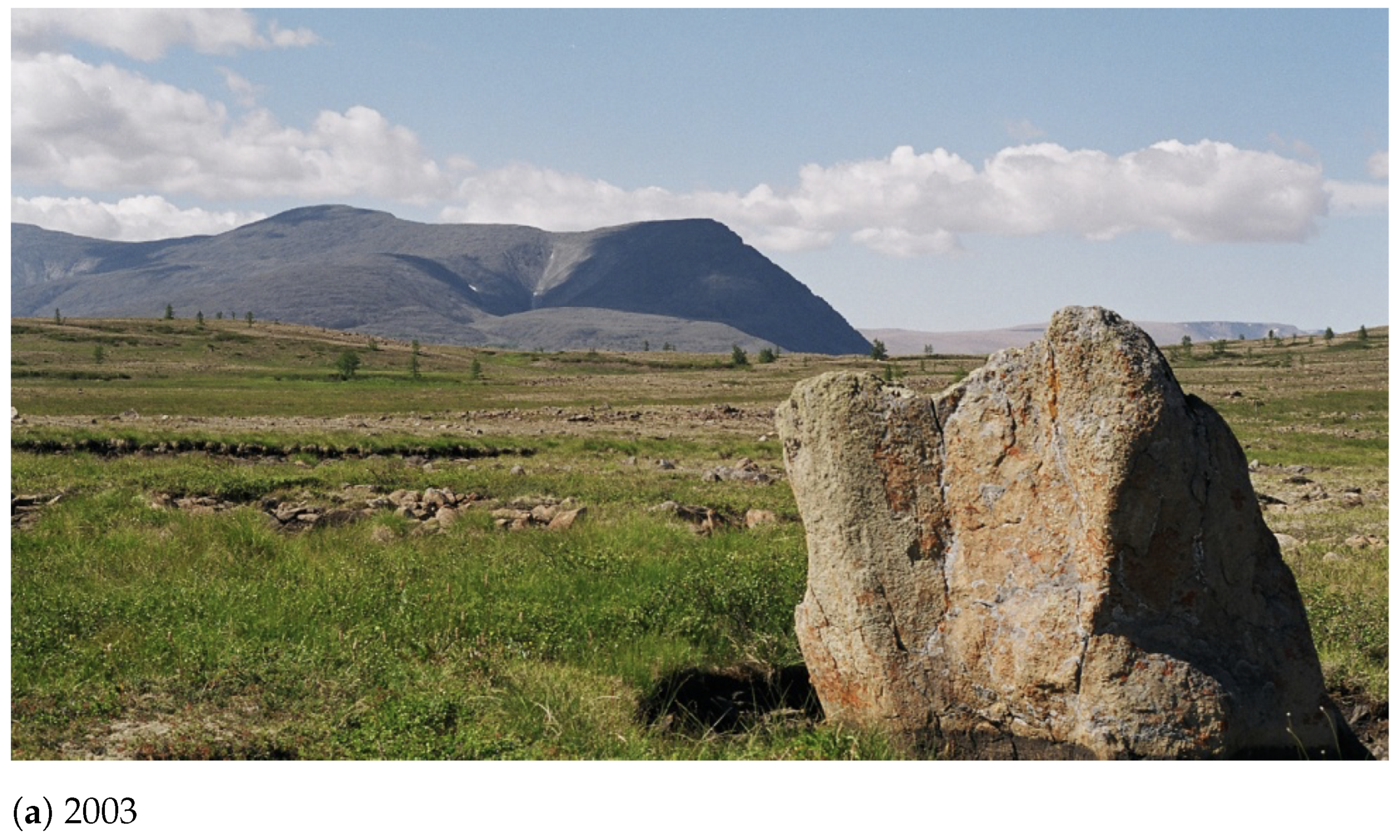
While moving, the ice masses traveled between two mountains composed of gabbro—the Chernaya and Malaya Chernaya mountains. The large relief formed along the glacier path in this location facilitated the portage, mixing, and accumulation of two ultrabasic rock types, namely yellow-orange-type peridotites and grey gabbro, on the site (Figure 2).
The upper treeline ecotone is dominated by pure Siberian larch (Larix sibirica Ledeb.) forests. The lower part of the ecotone features open larch forests and forests with admixed Siberia spruce (Picea obovata Ledeb.) and mountain birch (Betula tortuosa Ledeb.). The undergrowth features dwarf birch (Betula nana L.) and Siberian juniper (Juniperus sibirica L.).
2.2. Ground Measurements
Nine circular forest plots with a radius equal to 11 m were identified in the study area. Measurements were made to determine the location of each individual Siberian larch: trees, undergrowth, and sprouts. The following biometrical characteristics were determined for each specimen of Siberian larch: diameter at root collar, DBH, and maximum radius of crown projection calculated on the basis of the crown length measured in two orthogonal directions. The height of the large trees was determined using a Suunto clinometer (Suunto Inc., Vantaa, Finland), and small trees, undergrowth, and sprouts were measured using a measurement tape.
2.3. Tree Recognition
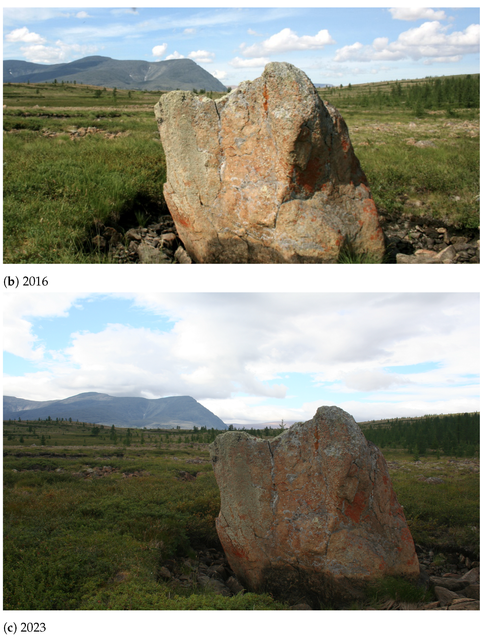
The research included the recognition and digitalization of the trees present in images from the 1960s and 2015. Trees that were not present in the 1960s images but appeared in 2015 represented new generations of Siberian larch. Figure 3 features fragments of a 1964 aerial photo and 2015 satellite image, allowing an assessment of their resolving power for tree recognition.
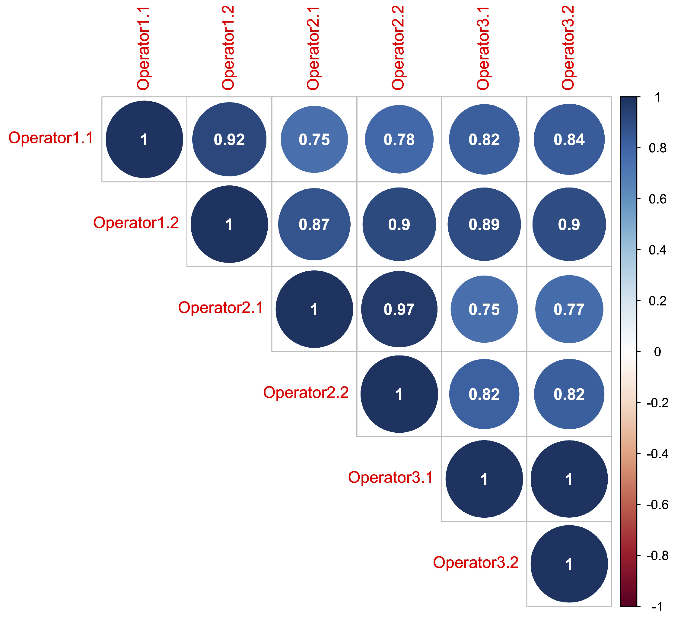
Within each of the nine forest plots, three operators twice performed tree recognition based on satellite images. After this, an agreement analysis was performed for the results of the tree recognition using first and second recognition variants for all operators, and among the operators using the Spearman correlation coefficient. The results of the agreement analysis of tree recognition by the operators for the test sites are shown in Figure 4. The time interval between the attempts was no shorter than four hours. All the values of the Spearman coefficient were valid at the level of 0.05 or above. Variance analysis was also performed for the number of trees found by the operators. The lowest variance in the number of trees was found between operators 1 and 2.
A study area map with the forest plot locations and distribution of trees in the early 1960s and early 21st century is shown in Figure 5.
2.4. Forest–Tundra Patch Delineation
The previously performed large-scale mapping of forest–tundra biocoenoses using the ocular estimation method [8,9] employed an approach based on selecting phytocoenohoras—areas that were relatively homogenous in terms of one or several vegetation components and/or the specifics of forest growth conditions. The current work used tree density as a criterion for distinguishing patches of closed forest, open forest, light forest, and tundra with single trees. In his field work, S.G. Shiyatov [8] used the average distance between the trees as a threshold value. Sites were considered dense forest if the average distance among the trees was less than 7–10 m; for woodlands, the values of this parameter ranged from 10 to 30 m; for sparse stands they ranged from 30 to 60 m; and for tundra with isolated trees the values were over 60 m.
In the current work, the authors used threshold values corresponding to the midpoints of the ranges described above to distinguish the following types: closed forest (up to and including 8.5 m); open forest (8.5–25 m); light forest (25–55 m); and tundra with single trees (over 55 m).
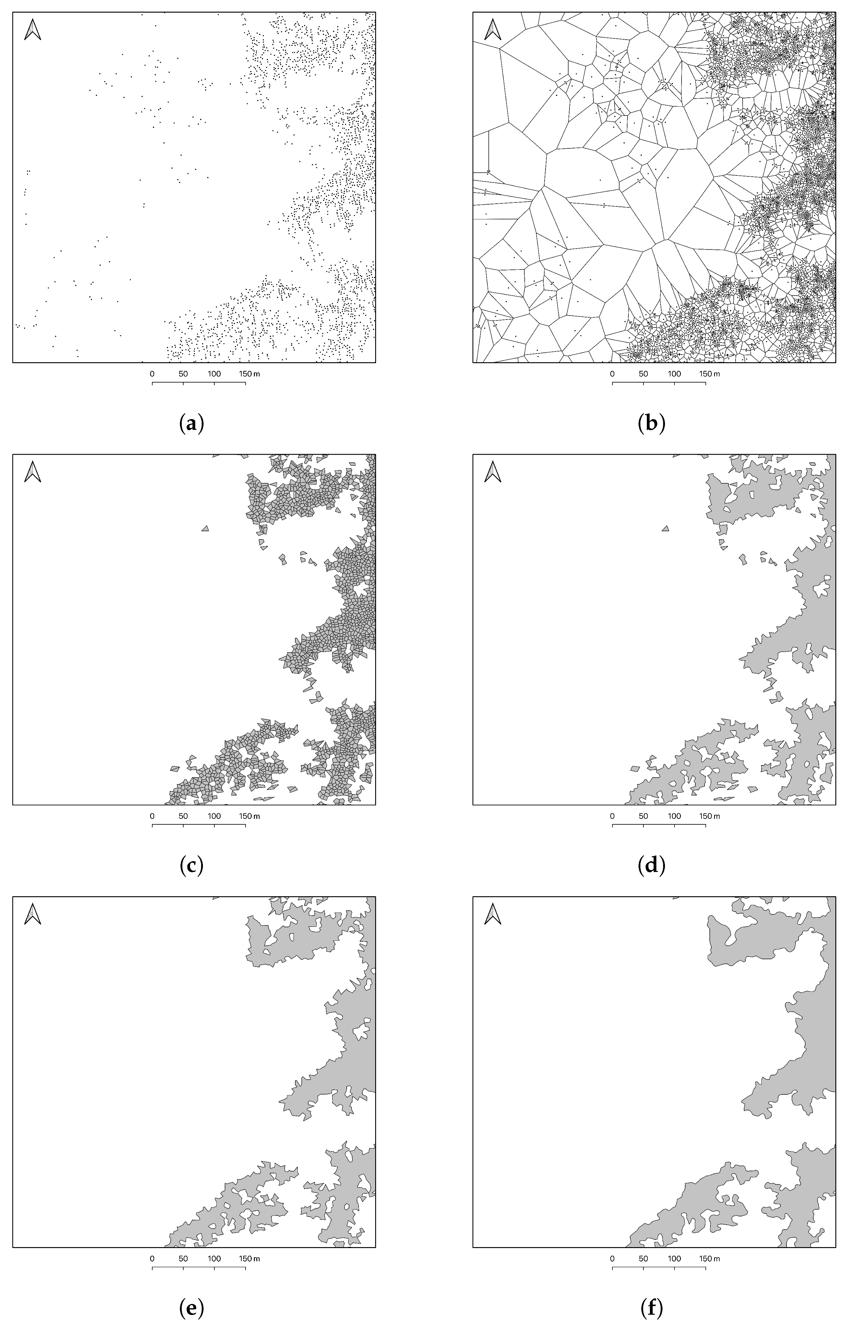
In order to create maps of the phytocoenohoras in the early 1960s and 2015, the authors used a developed method. Figure 6 shows maps illustrating the key steps of the method. Step 1 included using a layer of points (Figure 6a) describing the location of the trees to create a layer of Voronoi polyhedrons (Figure 6b). Step 2 included selecting cells representing one phytocoenohora type using cell areas (Figure 6c). The next step included merging cells into larger polygons by removing internal boundaries (Figure 6d) and subsequently filtering by the area value (Figure 6e). Filtering was required to exclude small-area polygons and prevent the occurrence of degenerated cases. For example, if a merged polygon displayed properties of a forest, but its area was too small, meaning that it contained a small number of trees, it could not be considered a closed forest. The final step included the smoothing of polygonal boundaries, which allowed the removal of polyline fragments that appeared at the nexus of three or more Voronoi polyhedrons (Figure 6f). The results of applying the described method included maps of phytocoenohora types for the 1960s and 2015.
Figure 6.
Main steps of selecting phytocoenohora types for “closed forest” type: (a)—distribution of the trees on the site (see area of interest in Figure 5); (b)—breaking area of interest into Voronoi polygons; (c)—selecting cells belonging to the same phytocoenohora type using area values; (d)—joining cells into larger polygons by removing internal boundaries; (e)—deleting small-area polygons to exclude degenerated cases; (f)—smoothing polygon boundaries.

The sources of larch tree location data in the study area included halftone aerial photographs taken in 1962 and 1964 and a high-resolution satellite image taken in 2015. All images were georeferenced using QGIS (https://qgis.org/, accessed on 2 November 2022). The spatial resolution of the aerial and satellite images allowed us to decipher trees taller than four meters. Digitalization was used to form vector-based layers of points in QGIS, where each dot corresponded to tree positions in 1962/1964 and 2015 (Figure 5). Data processing was performed using R software v. 4.1.2. (the R Foundation, Austria, Vienna) (https://www.r-project.org/, accessed on 2 November 2023).
3. Results
The far central part of Figure 2 demonstrates an increase in the size of existing trees and the appearance of new trees in parts of the mountain tundra within the past 20 years. The tree location data obtained in the course of deciphering aerial images from 1962 and 1964 and the 2015 satellite image demonstrated that the number of trees within the study almost doubled from early 1960 to 2015 (from 14,377 to 28,344).
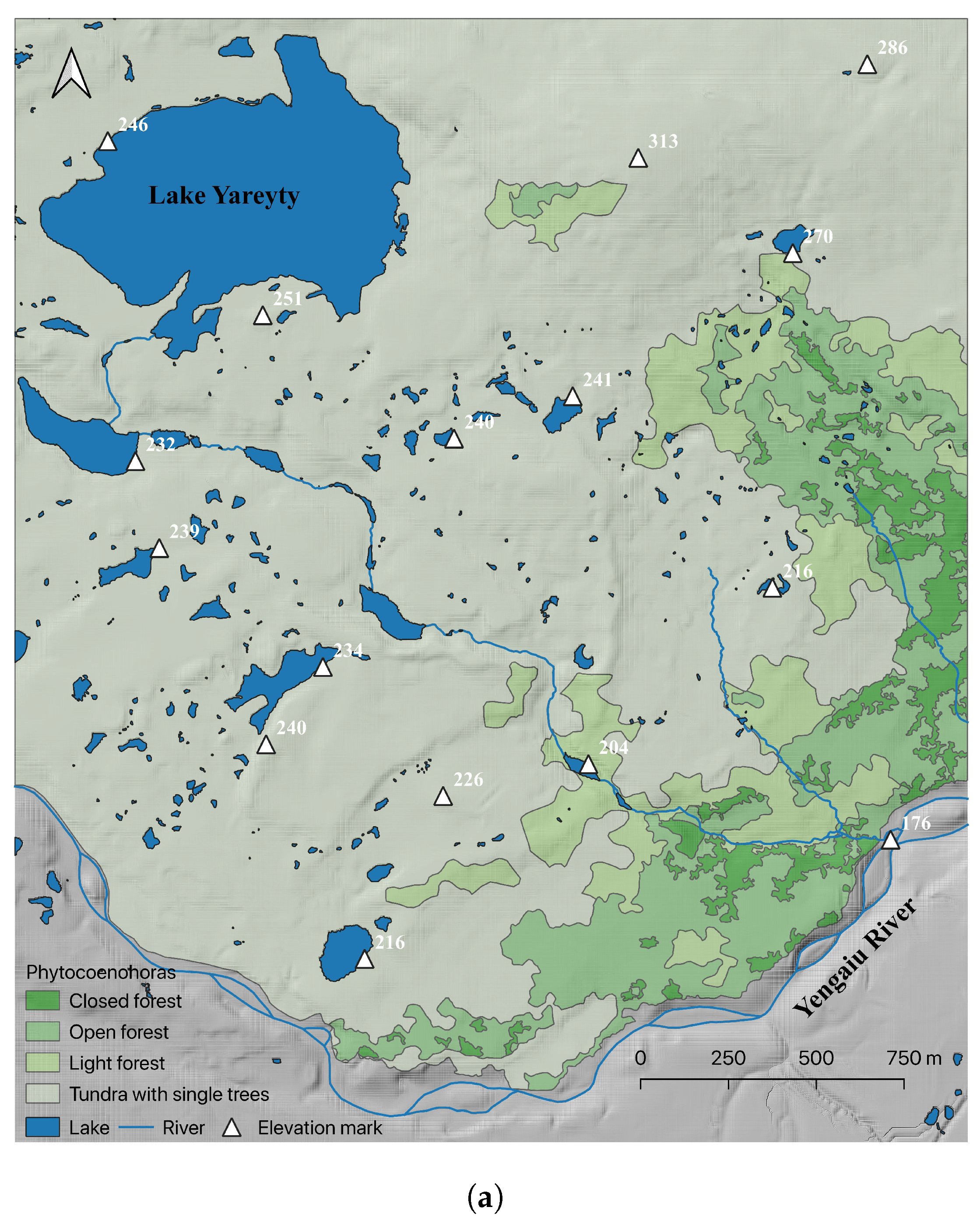
Figure 7 displays distribution maps of the main phytocoenohora types in the study area for the early 1960s (Figure 7a) and for 2015 (Figure 7b), developed using the previously described method. The area of closed forest during this period increased by 28.1 hectares (from 21.5 to 49.6 ha), that of open forest by 25.7 ha (from 70.5 to 96.2 ha), and that of light forest by 59.1 ha (from 55.3 to 114.4 ha). The area of tundra with single trees decreased by 112.9 ha (from 585.7 to 472.8 to). Considering the percentage of the total study area, the shares of closed forest, open forest, and light forest increased from 2.9% to 6.8%, from 9.6% to 13.1%, and from 7.5% to 15.6%, respectively, while the share of tundra with single trees decreased from 79.9% to 64.5% (Table 1).
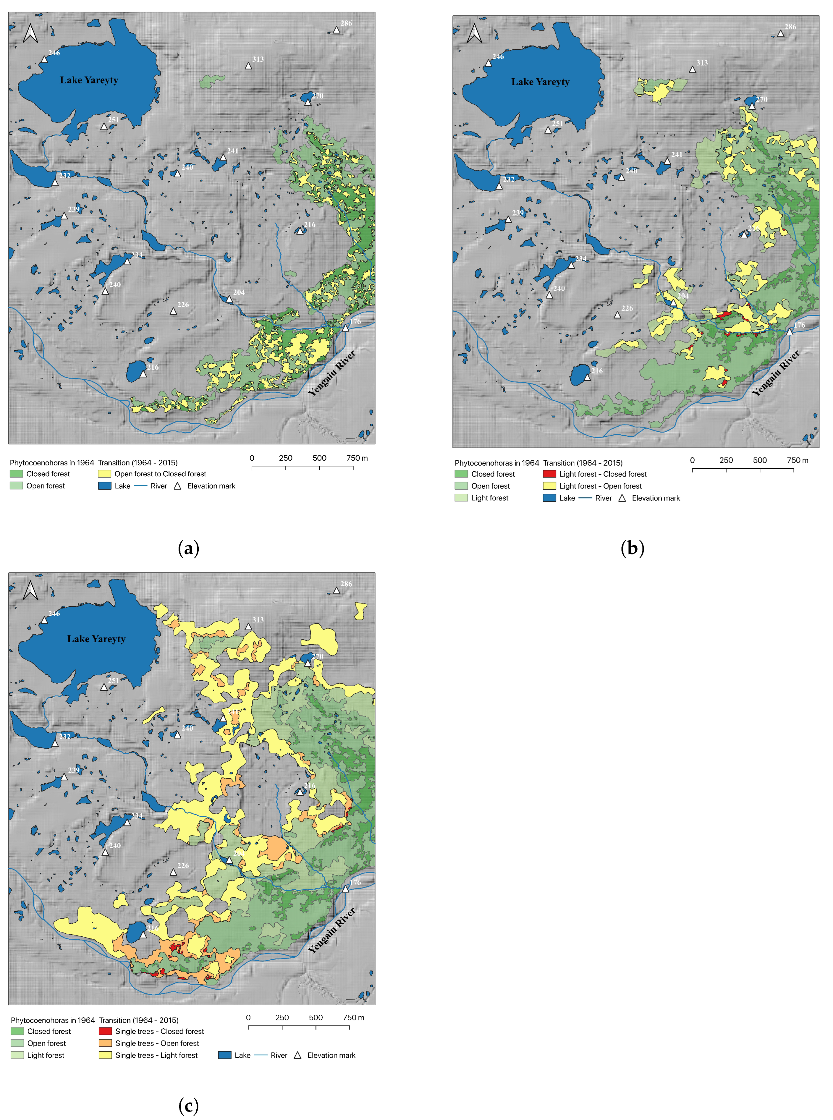
Figure 8 includes maps that describe the transitions from one phytocoenohora type to another from the early 1960s until 2015. Table 2 contains data on the ratio of the total area of the lots occupied by each phytocoenohora type at the beginning and at the end of the period in question. Over all, the phytocoenohora type transitions occurring from the early 1960s to 2015 can be described as moving from lower-density types to higher-density ones. At the same time, the areas of the lots featuring transitions between neighboring types, e.g., “open forest–closed forest”, “light forest–open forest”, or “tundra with single trees–light forest”, were bigger than those of the lots with more radical transitions, for example, “tundra with single trees–closed forest” and “light forest–closed forest”. Figure 8 demonstrates that lots displaying the latter transitions were mainly located in the southern part of the study area. Backward transitions, e.g., from closed forest to open forest, light forest, or tundra with single trees, were not found for the period in question.
4. Discussion
A comparative analysis of the number of trees for the early 1960s and 2015 demonstrated that local climate warming in the Polar Urals [24] facilitated both the appearance of a young Siberian larch generation and the survival of new trees in previously deforested or sparsely forested parts of the tundra as well as in lots where trees grew before. Several methodological issues arise in the course of the formalized description and representation of changes occurring within upper-treeline ecotones. These issues are due to the fact that ecotone characteristics depend upon the level of detail used in ecotone studies [25,26,27]. This is caused by the properties of vegetation, which itself represents a complex multiscale phenomenon. A consideration of these specifics in ecological research, including the use of abstraction, is crucial for understanding the dependencies and processes related to vegetation [13,16,28].
Upper-treeline representation in the form of a line describing the beginning and end of the period of interest allows the implementation of methods for the automated evaluation of horizontal and vertical shifts using “algebra of maps” geoinformation system functions [9,29]. The limitations of this approach reveal themselves on sites with a low density of trees. In this case, the representation of the forest boundary as a continuous line is complicated or even impossible, sometimes due to the presence of pockets—fragments of forest, open forest, or light forest that are located at a distance from the large wooded lots. At the same time, the spatial superposition of the layers with phytocoenohora types representing the beginning and end of the period in question allows the localization of phytocoenohora type transition areas. The suggested method for mapping phytocoenohora types in the upper-treeline ecotone has no limitations similar to those described above. It is highly universal and decreases the subjectivity of selecting vegetation cover units. This method for selecting and mapping phytocoenohora types allowed us to illustrate the characteristic effects and spatial patterns in the distribution and spread of trees into barren or sparsely wooded parts of the study area. The characteristic trend for the mountain massifs of the Northern Urals and Siberia, as well as North America, features the expansion of Larix species into mountain tundra and an increase in the tree density of wooded slope areas [3,6,30]. The maps shown in Figure 8 allowed us to assess the specifics of these processes in the study area. Generally, the “open forest–closed forest” transition could be characterized as the infilling of the openings within the closed forest, open forest, or their combination (Figure 8a). The “light forest–closed forest” and “tundra with single trees–closed forest” transitions also occurred in small patches surrounded by tree stands with a relatively high density (Figure 8b and Figure 8c). The scale of Siberian larch expansion into treeless or sparsely wooded parts of the mountain tundra, representing a “shift” in vegetation boundaries, could be observed on lots with a “light forest–open forest” transition (Figure 8b) and a transition from tundra with single trees to light forest or open forest (Figure 8c). The approach for assessing changes in the upper-treeline ecotone described in this work corresponds to a certain degree with an approach based upon selecting areas of the expansion, retraction, and stable population of trees on sites close to the upper treeline in the Pyrenees [31], however, we used a higher level of detail in our work.
Under a certain combination of microclimatic factors, larch can survive under unfavorable conditions in its creeping form, changing into the stem form with an improvement in the environmental conditions [32]. This means that the considered patches could be refuges where Siberian larch survived the unfavorable cooling period. This could explain the formation and increase in size of open forest and light forest patches far away from the patches of phytocoenohoras forming a relatively continuous band of open forest and closed forest (Figure 7).
The appearance of the seedlings and their survival under harsh soil and climatic conditions close to the upper treeline is driven by a complex combination of environmental factors [33,34,35]. It was previously found that wind and snow have a critical impact on tree survival and growth in this region. The blowing of snow away from the upper parts of landforms causes deep soil freezing, which has a negative impact on young trees. For example, research into the effects of snow depth on soil temperature in the circumpolar tundra-to-forest transition zone of the Canadian north-east demonstrated that the soil in the forests did not freeze until January, with a following temperature decline to a minimum of −1 degree centigrade in March. In tundra, the soil froze down to 9 centimeters in mid-November, with the temperature dropping in March to a minimum below −11 °C, which was about 10 °C below the values observed for the forest [36]. This was explained by the fact that the snow in the forest was 1.5–2 times deeper than in the tundra. Snow accumulation in the leeward parts of hills, knolls, and ridges can cause a later thaw and therefore shorten the vegetation period by several days or even weeks. Besides this, young trees suffer from snow-induced mechanical damage in cold periods.
Due to the substantial impacts of the north-western wind and snow on the survival and growth of trees, the formation of lots with trees occurs in stages through the development of biogroups and clumps of trees around grown larch exemplars, protecting younger trees from snow-related mechanical damage and facilitating snow accumulation, limiting the negative impacts of low soil and air temperatures on young trees [35,37]. Later on, an increase in tree density lowers the wind speed, which causes the formation of large snowdrifts on the leeward sides and has negative impacts on the survival of seedlings and young trees. As a result, open spots are formed, which are later populated with trees after the tree barrier shifts against the prevailing wind direction.
These specifics of the changing microclimatic conditions are displayed through the formation of tree bands [38,39]. As the tree barrier moves in the direction of the prevailing winds, the band of snowdrifts forming on the leeward side shifts in the same direction. In this case, the snow depth in the lots with previously excessive (for larch survival) snow accumulation gradually decreased, and conditions became more favorable for larch survival and growth. The same role is played by landforms. Ridges and knolls formed by glaciers and large stones can also protect young larch trees from wind and snow. At the same time, trees attach to the middle of ridge slopes in wind shadow areas, where conditions are more optimal in terms of soil freezing (snow accumulates, but not in excessive amounts) and decreased snow-related mechanical damage (lower wind speeds). Figure 7b displays sparsely wooded lots surrounded by areas with a higher tree density. It can be expected that in the future these openings will be gradually populated by Siberian larch.
5. Conclusions
Maps of the locations of key phytocoenohora types (closed forest, open forest, light forest, and tundra with single trees) in the study area located on the south-eastern macroslope of the Rai-Iz massif (Polar Urals, Russia) for the early 1960s and 2015 were produced using data from aerial and satellite images, processed via an original method for the automated recognition of lots with a relatively uniform density of larch trees. It was found that in the past half-century, the number of trees in the study area almost doubled. The relative area of lots belonging to the tundra with single trees phytocoenohora decreased by 15.4% due to the increase in the areas of light forest (8.1%), open forest (3.5%), and closed forest (3.8%). At the same time, the transition from open forest to closed forest mainly occurred on sites within the forest-covered territory, so the process could be described as “infilling”. The replacement of the tundra with single trees and light forest phytocoenohora types with open forest represented the expansion of larch into the mountain tundra. The grown trees provided natural protection from wind and snow for younger trees. This explained the formation of biogroups and clumps of trees around the grown larch exemplars, followed by their joining with neighboring groups or clumps. When trees formed a barrier protecting young generations from the negative impacts of snow-related mechanical damage, new tree generations appeared on patches at the leeward side of these barriers. Then, Siberian larch gradually filled the “openings”.
Author Contributions
Conceptualization, V.F. and A.M.; formal analysis, V.F.; methodology, V.F. and A.M.; data curation, A.M. and V.F.; software, V.F.; visualization, V.F.; project administration, A.M. and V.F.; writing—original draft, A.M. and V.F.; writing—review and editing, V.F. and A.M. All authors have read and agreed to the published version of the manuscript.
Funding
This research was collaboratively funded by the Russian Ministry for Science and Education (project No. FEUG-2023-0002). The approach for analyzing patches of phytoenochora transition was developed within the framework of the Russian Ministry for Science and Education (project No. FEUZ-2023-0023).
Data Availability Statement
The data are provided in the article.
Conflicts of Interest
The authors declare no conflict of interest.
References
- Shiyatov, S.G. Reconstruction of climate and the upper timberline dynamics since AD 745 by tree-ring data in the Polar Ural Mountains. In Proceedings of the International Conference on Past, Present and Future Climate, Helsinki, Finland, 22–25 August 1995; pp. 144–147. [Google Scholar]
- Kullman, L. Tree line population monitoring of Pinus sylvestris in the Swedish Scandes, 1973–2005: Implications for tree line theory and climate change ecology. J. Ecol. 2007, 95, 41–42. [Google Scholar] [CrossRef]
- Hagedorn, F.; Shiyatov, S.G.; Mazepa, V.S.; Devi, N.M.; Grigor’ev, A.A.; Bartish, A.A.; Fomin, V.V.; Kapralov, D.S.; Terent’ev, M.; Bugman, H.; et al. Treeline advances along the Urals mountain range—Driven by improved winter conditions? Glob. Chang. Biol. 2014, 20, 3530–3543. [Google Scholar] [CrossRef] [PubMed]
- Hellmann, L.; Agafonov, L.; Ljungqvist, F.C.; Churakova (Sidorova), O.; Düthorn, E.; Esper, J.; Hülsmann, L.; Kirdyanov, A.V.; Moiseev, P.; Myglan, V.S.; et al. Diverse growth trends and climate responses across Eurasia’s boreal forest. Environ. Res. Lett. 2016, 11, 074021. [Google Scholar] [CrossRef]
- Pellizzari, E.; Camarero, J.J.; Gazol, A.; Granda, E.; Shetti, R.; Wilmking, M.; Moiseev, P.; Pividori, M.; Carrer, M. Diverging shrub and tree growth from the Polar to the Mediterranean biomes across the European continent. Glob. Chang. Biol. 2017, 23, 3169–3180. [Google Scholar] [CrossRef] [PubMed]
- Mamet, S.D.; Brown, C.D.; Trant, A.J.; Laroque, C.P. Shifting global Larix distributions: Northern expansion and southern retraction as species respond to changing climate. J. Biogeogr. 2019, 46, 30–44. [Google Scholar] [CrossRef]
- Seastedt, T.R.; Oldfather, M.F. Climate change, ecosystem processes and biological diversity responses in high elevation communities. Climate 2021, 9, 87. [Google Scholar] [CrossRef]
- Shiyatov, S.G. Rates of Change in the Upper Treeline Ecotone in the Polar Ural Mountains. Pages News 2003, 11, 8–10. [Google Scholar] [CrossRef]
- Shiyatov, S.G.; Terent’ev, M.M.; Fomin, V.V.; Zimmermann, N.E. Altitudinal and horizontal shifts of the upper boundaries of open and closed forests in the Polar Urals in the 20th century. Russ. J. Ecol. 2007, 38, 223–227. [Google Scholar] [CrossRef]
- Kharuk, V.I.; Ranson, K.J.; Im, S.T.; Vdovin, A.S. Spatial distribution and temporal dynamics of high-elevation forest stands in southern Siberia. Glob. Ecol. Biogeogr. 2010, 19, 822–830. [Google Scholar] [CrossRef]
- Petrov, I.A.; Kharuk, V.I.; Dvinskaya, M.L.; Im, S.T. Reaction of coniferous trees in the Kuznetsk Alatau alpine forest-tundra ecotone to climate change. Contemp. Probl. Ecol. 2015, 8, 423–430. [Google Scholar] [CrossRef]
- Hansson, A.; Dargusch, P.; Shulmeister, J. A review of modern treeline migration, the factors controlling it and the implications for carbon storage. J. Mt. Sci. 2021, 18, 291–306. [Google Scholar] [CrossRef]
- Kark, S.; van Rensburg, B.J. Ecotones: Marginal or central areas of transition? Isr. J. Ecol. Evol. 2006, 52, 29–53. [Google Scholar] [CrossRef]
- Chiu, C.-A.; Lee, M.-F.; Tzeng, H.-Y.; Liao, M.-C. A concise scheme of vegetation boundary terms in subtropical high mountains. Afr. J. Agric. Res. J. Ecol. Evol. 2014, 9, 1560–1570. [Google Scholar] [CrossRef]
- Jobbágy, E.G.; Jackson, R.B. Global controls of forest line elevation in the northern and southern hemispheres. Glob. Ecol. Biogeogr. 2000, 9, 253–268. [Google Scholar] [CrossRef]
- Holtmeier, F.-K.; Broll, G. Treelines—Approaches at Different Scales. Sustainability 2017, 9, 808. [Google Scholar] [CrossRef]
- Smith, W.K.; Germino, M.J.; Hancock, T.E.; Johnson, D.M. Another perspective on altitudinal limits of alpine timberlines. Tree Physiol. 2003, 23, 1101–1112. [Google Scholar] [CrossRef] [PubMed]
- Körner, C. A re-assessment of high elevation treeline positions and their explanation. Oecologia 1998, 115, 445–459. [Google Scholar] [CrossRef]
- Jain, A.K.; Murty, M.N.; Flynn, P.J. Data clustering: A review. ACM Comput. Surv. 1999, 31, 264–323. [Google Scholar] [CrossRef]
- Fortin, M.-J. Edge Detection Algorithms for Two-Dimensional Ecological Data. Ecology 1993, 75, 956–965. [Google Scholar] [CrossRef]
- Fortin, M.J.; Drapeau, P. Delineation of Ecological Boundaries: Comparison of Approaches and Significance Tests. Oikos 1995, 72, 323–332. [Google Scholar] [CrossRef]
- Gonzalez, R.C.; Woods, R.E. Digital Image Processing, 4th ed.; Pearson: New York, NY, USA, 2018; pp. 812–902. [Google Scholar]
- Clarke, C.L.; Edwards, M.E.; Gielly, L.; Ehrich, D.; Hughes, P.D.M.; Morozova, L.M.; Haflidason, H.; Mangerud, J.; Svendsen, J.I.; Alsos, I.G. Persistence of arctic-alpine flora during 24,000 years of environmental change in the Polar Urals. Sci. Rep. 2020, 9, 19613. [Google Scholar] [CrossRef] [PubMed]
- Shalaumova, Y.V.; Fomin, V.V.; Kapralov, D.S. Spatiotemporal dynamics of the Urals’ climate in the second half of the 20th century. Russ. Meteorol. Hydrol. 2010, 35, 107–114. [Google Scholar] [CrossRef]
- Gosz, J.R. Ecotone Hierarchies. Ecol. Appl. 1993, 3, 369–376. [Google Scholar] [CrossRef] [PubMed]
- Fortin, M.-J.; Olson, R.J.; Ferson, S.; Iverson, L.; Hunsaker, C.; Edwards, G.; Klemas, V. Issues related to the detection of boundaries. Landsc. Ecol. 2000, 15, 453–466. [Google Scholar] [CrossRef]
- Hufkens, K.; Scheunders, P.; Ceulemans, R. Ecotones in vegetation ecology: Methodologies and definitions revisited. Ecol. Res. 2009, 24, 977–986. [Google Scholar] [CrossRef]
- Bateson, G. Mind and Nature: A Necessary Unity, 3rd ed.; E. P. Dutton: New York, NY, USA, 1979; pp. 16–229. [Google Scholar]
- Singh, C.P.; Panigrahy, S.; Thaplya, A.; Kimothi, M.M.; Soni, P.; Parihar, J.S. Monitoring the alpine treeline shift in parts of the Indian Himalayas using remote sensing. Curr. Sci. 2012, 102, 559–562. [Google Scholar]
- Kirdyanov, A.V.; Hagedorn, F.; Knorre, A.A.; Fedotova, E.V.; Vaganov, E.A.; Naurzbaev, M.M.; Moiseev, P.A.; Rigling, A. 20th century tree-line advance and vegetation changes along an altitudinal transect in the Putorana Mountains, northern Siberia. Boreas 2012, 41, 56–67. [Google Scholar] [CrossRef]
- Aulló-Maestro, I.; Gómez, C.; Hernández, L.; Camarero, J.J.; Sánchez-González, M.; Cañellas, I.; Vázquez de la Cueva, A.; Montes, F. Monitoring montane-subalpine forest ecotone in the Pyrenees through sequential forest inventories and Landsat imagery. Ann. For. Sci. 2023, 80, 32. [Google Scholar] [CrossRef]
- Devi, N.; Hagedorn, F.; Moiseev, P.; Bugmann, H.; Shiyatov, S.; Mazepa, V.; Rigling, A. Expanding forests and changing growth forms of Siberian larch at the Polar Urals treeline during the 20th century. Glob. Chang. Biol. 2008, 14, 1581–1591. [Google Scholar] [CrossRef]
- Holtmeier, F.K.; Broll, G. Treeline research-from the roots of the past to present time. A review. Forests 2020, 11, 38. [Google Scholar] [CrossRef]
- Cudlín, P.; Klopčič, M.; Tognetti, R.; Máliš, F.; Alados, C.L.; Bebi, P.; Grunewald, K.; Zhiyanski, M.; Andonowski, V.; Porta, N.L.; et al. Drivers of treeline shift in different European mountains. Clim. Res. 2017, 73, 135–150. [Google Scholar] [CrossRef]
- Mathisen, I.E.; Mikheeva, A.; Tutubalina, O.V.; Aune, A.; Hofgaard, A. Fifty years of tree line change in the Khibiny Mountains, Russia: Advantages of combined remote sensing and dendroecological approachesy. Appl. Veg. Sci. 2014, 17, 6–16. [Google Scholar] [CrossRef]
- Lackner, G.; Domine, F.; Nadeau, D.; Lafaysse, M.; Lackner, G.; Domine, F.; Nadeau, D.; Lafaysse, M.; Dumont, M.; Lackner, G.; et al. Snow properties at the forest—Tundra ecotone: Predominance of water vapor fluxes even in deep, moderately cold snowpacks. Cryospherei 2022, 16, 3357–3373. [Google Scholar] [CrossRef]
- Kharuk, I.V.; Im, S.T.; Dvinskaya, M.L.; Ranson, K.J. Climate-induced mountain tree-line evolution in southern Siberia. Scand. J. For. Res. 2010, 25, 446–454. [Google Scholar] [CrossRef]
- Fomin, V.V.; Shiyatov, S.G. Factors determining the phenomena in the upper tree line ecotone in the Polar Urals mountains. For. Russ. Econ. Them 2021, 16, 42–51. [Google Scholar] [CrossRef]
- Holtmeier, F.-K. Relocation of snow and its effects in the treeline ecotone—With special regard to the Rocky mountains, the Alps and Northern Europe. Cryospherei 2005, 136, 343–373. [Google Scholar]
Figure 1.
Study area.

Figure 2.
Repeated landscape photos. On the far left is Chernaya mountain; photos (a,c) include fragments of the Rai-Iz massif (far center). Photo (a) was taken by S.G. Shiyatov on 14 June 2003, photo (b) by A.P. Mihailovich on 14 July 2016, and photo (c) by V.V. Fomin on 9 August 2023.
Figure 2.
Repeated landscape photos. On the far left is Chernaya mountain; photos (a,c) include fragments of the Rai-Iz massif (far center). Photo (a) was taken by S.G. Shiyatov on 14 June 2003, photo (b) by A.P. Mihailovich on 14 July 2016, and photo (c) by V.V. Fomin on 9 August 2023.


Figure 3.
Fragments of 1964 aerial photo (a) and 2015 satellite image (b).

Figure 4.
Correlation matrix with Spearman coefficient values used to assess agreement of tree recognition by three operators. The first digit represents the operator, and the second digit the recognition variant used by this operator. All coefficient values were valid at the level of 0.05 or above.

Figure 5.
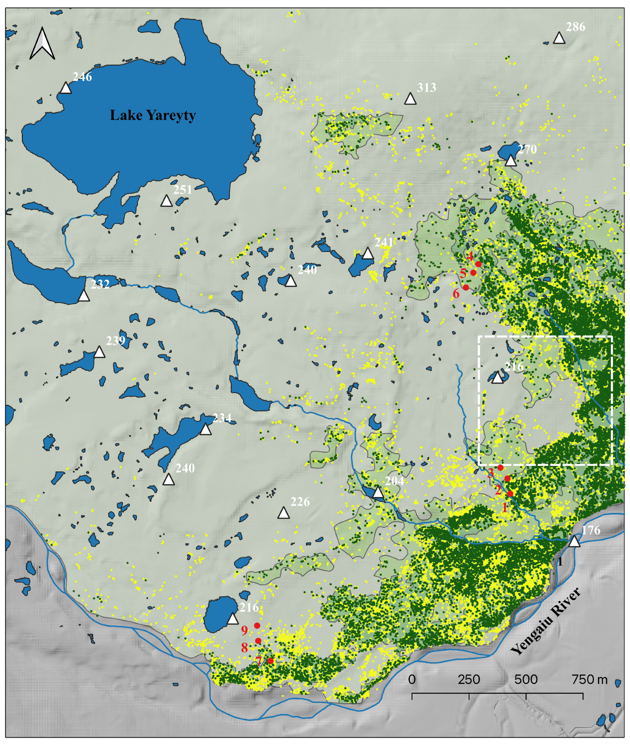
Study area map including shaded relief and elevation marks. Green dots indicate trees in the early 1960s, yellow dots indicate new trees identified in the satellite image of 2015, and red dots indicate forest plots. The rectangle formed by the white dotted line represents the area of interest shown in Figure 6, illustrating the stages of the algorithm for allocating areas of a certain type of phytocenochora.
Figure 5.
Study area map including shaded relief and elevation marks. Green dots indicate trees in the early 1960s, yellow dots indicate new trees identified in the satellite image of 2015, and red dots indicate forest plots. The rectangle formed by the white dotted line represents the area of interest shown in Figure 6, illustrating the stages of the algorithm for allocating areas of a certain type of phytocenochora.

Figure 7.
Maps of the main phytocoenohora types (closed forest, open forest, light forest, and tundra with single trees) present in the study area for the early 1960s (a) and 2015 (b).
Figure 7.
Maps of the main phytocoenohora types (closed forest, open forest, light forest, and tundra with single trees) present in the study area for the early 1960s (a) and 2015 (b).


Figure 8.
Maps describing spatial location of the lots featuring phytocoenohora type transitions from 1960s to 2015: (a) from open forest to closed forest; (b) from light forest to closed forest and from light forest to open forest; (c) from tundra with single trees to closed forest, open forest, or light forest.


Table 1.
Areas occupied by different phytocoenohora types within the study area in 1964 and 2015.
| Area, ha/ % | |||
|---|---|---|---|
| Phytocoenohora | 1964 | 2015 | Δ (2015–1964) |
| Closed forest | 21.5/2.9 | 49.6/6.8 | 28.1/3.8 |
| Open forest | 70.5/9.6 | 96.2/13.1 | 25.7/3.5 |
| Light forest | 55.3/7.5 | 114.4/15.6 | 59.1/8.1 |
| Tundra with single trees | 585.7/79.9 | 472.8/64.5 | −112.9/−15.4 |
Table 2.
Areas of different phytocoenohora types in 1964 and 2015: transition (no transition) areas.
Table 2.
Areas of different phytocoenohora types in 1964 and 2015: transition (no transition) areas.
| Phytocoenohora Types | |||
|---|---|---|---|
| Num | 1964 | 2015 | Area, ha |
| 1 | Closed forest | Closed forest | 21.5 |
| 2 | Open forest | Closed forest | 25.8 |
| 3 | Open forest | Open forest | 44.7 |
| 4 | Light forest | Closed forest | 1.1 |
| 5 | Light forest | Open forest | 28.1 |
| 6 | Light forest | Light forest | 26.1 |
| 7 | Tundra with single trees | Closed forest | 1.2 |
| 8 | Tundra with single trees | Open forest | 23.4 |
| 9 | Tundra with single trees | Light forest | 88.3 |
| 10 | Tundra with single trees | Tundra with single trees | 472.8 |
Disclaimer/Publisher’s Note: The statements, opinions and data contained in all publications are solely those of the individual author(s) and contributor(s) and not of MDPI and/or the editor(s). MDPI and/or the editor(s) disclaim responsibility for any injury to people or property resulting from any ideas, methods, instructions or products referred to in the content. |
© 2023 by the authors. Licensee MDPI, Basel, Switzerland. This article is an open access article distributed under the terms and conditions of the Creative Commons Attribution (CC BY) license (https://creativecommons.org/licenses/by/4.0/).
Share and Cite
MDPI and ACS Style
Mikhailovich, A.; Fomin, V. Quantitative Assessment of Forest–Tundra Patch Dynamics in Polar Urals Due to Modern Climate Change. Forests 2023, 14, 2340. https://doi.org/10.3390/f14122340
AMA Style
Mikhailovich A, Fomin V. Quantitative Assessment of Forest–Tundra Patch Dynamics in Polar Urals Due to Modern Climate Change. Forests. 2023; 14(12):2340. https://doi.org/10.3390/f14122340
Chicago/Turabian StyleMikhailovich, Anna, and Valery Fomin. 2023. "Quantitative Assessment of Forest–Tundra Patch Dynamics in Polar Urals Due to Modern Climate Change" Forests 14, no. 12: 2340. https://doi.org/10.3390/f14122340
Note that from the first issue of 2016, this journal uses article numbers instead of page numbers. See further details here.