
Supporting Operational Tree Marking Activities through Airborne LiDAR Data in the Frame of Sustainable Forest Management


Laboratory of Forest Management and Remote Sensing, School of Forestry and Natural Environment, Aristotle University of Thessaloniki, 54124 Thessaloniki, Greece
*
Author to whom correspondence should be addressed.
Forests 2023, 14(12), 2311; https://doi.org/10.3390/f14122311
Submission received: 4 October 2023
/
Revised: 16 November 2023
/
Accepted: 21 November 2023
/
Published: 24 November 2023
(This article belongs to the Special Issue Application of Laser Scanning Technology in Forestry)
Abstract
:Implementing adaptation and mitigation strategies in forest management constitutes a primary tool for climate change mitigation. To the best of our knowledge, very little research so far has examined light detection and ranging (LiDAR) technology as a decision tool for operational cut-tree marking. This study focused on investigating the potential of airborne LiDAR data in enhancing operational tree marking in a dense, multi-layered forest over complex terrain for actively supporting long-term sustainable forest management. A detailed tree registry and density maps were produced and evaluated for their accuracy using field data. The derived information was subsequently employed to estimate additional tree parameters (e.g., biomass and tree-sequestrated carbon). An integrated methodology was finally proposed using the developed products for supporting the time- and effort-efficient operational cut-tree marking. The results showcased the low detection ability (R2 = 0.15–0.20) of the trees with low DBH (i.e., regeneration and understory trees), while the dominant trees were accurately detected (R2 = 0.61). The stem biomass was accurately estimated, presenting an R2 of 0.67. Overall, despite some products’ low accuracy, their full and efficient exploitability within the aforementioned proposed methodology has been endeavored with the aim of actively contributing to long-term sustainable forest management.
1. Introduction
Forests’ existence and health strongly depend on climate change and its’ ever-increasing global impacts [1]. The elevated temperature and reduced precipitation affect forest growth and productivity while increasing the occurrence and intensity of extreme wildfires, which result in additional loss of forest cover worldwide [2]. Scientific predictions suggest that global warming and subsequent severe drought will have further catastrophic impacts on forest ecosystems [3]. In addition, it is widely recognized that climate change mitigation cannot be accomplished without the contribution of forests since they constitute a large carbon sink, storing 90% of the total carbon (C) in natural terrestrial ecosystems [4]. As such, climate change’s speed makes implementing adaptation and mitigation strategies in forest management highly important [5]. In fact, sustainable forest management is a primary tool for forest conservation and, consequently, preserving an environment suitable for human life.
An integral part of sustainable forest management is the forest management plan, conducted for a given forest area every 5 to 20 years [6]. Forest inventory is the first step for creating a comprehensive forest management plan [7] and is used—among others—for cut-tree marking (i.e., marking of trees to be harvested), a vital activity defining the forest management success and, thus, the future stand development [8,9]. Traditionally, selective tree marking, applied to multi-layered forests, is performed through labor-intensive and time-consuming fieldwork, including walking through the forested area to measure and identify the trees suitable for harvest. The typical tree-marking measurements include the diameter at breast height (DBH) and height estimation, which can be directly transformed into volume or biomass using allometric equations [10]. The difficulty in obtaining the necessary field-based information further increases in case areas of intense topography require inspection.
The use of remote sensing technology has provided an alternative solution for monitoring the forest environment and constitutes a valuable tool for developing forest inventories worldwide [11,12,13]. Light detection and ranging (LiDAR) sensors are successfully employed for this task since they can penetrate forest canopies and provide a three-dimensional representation of the Earth’s surface and its’ objects. Several studies have focused on using airborne laser scanning (ALS) data for accurate forest tree detection, leading to highly accurate results [14,15,16,17,18,19]. Actually, the ability of ALS-derived data to accurately identify tree tops and heights has provided researchers with the possibility to employ the tree detection results as reference/validation data [20]. Therefore, LiDAR technology enables the generation of a detailed tree registry over an entire forest area, providing accurate positional information on each individual tree. Except for the efficient cut-tree marking, the precise geographical location and height of ALS-detected trees constitute a fundamental source of information for the estimation of additional, vital for sustainable management, tree attributes, such as the diameter at breast height (DBH), the tree biomass (e.g., foliage and branches biomass), the tree sequestrated carbon and the potential surface fuel load (SFL, the dry weight of woody and non-woody organic material potentially created in case of logging a tree) [14,21,22]. As such, forest managers can use the additional estimated tree parameters to further assess the carbon- and SFL-related ecological impacts arising from each harvesting activity.
Despite the advantageous capabilities of LiDAR over other sensor types (e.g., optical and synthetic aperture radar (SAR)), high tree detection accuracy is not always a given. In fact, the effectiveness of forest tree detection through ALS data is inextricably linked to the LiDAR point cloud density and forest vegetation type and structure [23,24]. For instance, ALS-based tree detection has been proven to be more accurate in coniferous stands than in deciduous ones, while complex forest structures characterized by the intense presence of understory vegetation, high overstory tree density, or intense topography can significantly hinder the efficient detection of single trees [14,24]. Therefore, existing relevant research has been mostly conducted in specific parts of single-layered forests, plantations, or terrain of low relief, where forest conditions allow reliable identification of tree tops [14,17,20,23,25].
Although cut-tree marking activities play a pivotal role in the comprehensive management of forests at a global level, to the best of our knowledge, very few researchers have examined LiDAR data potential as a decision tool for operational cut-tree marking activities. The work of Contreras et al. (2012) constitutes a typical example of such application, where the effectiveness of thinning treatments was evaluated through modeling of tree-level fuel connectivity using LiDAR technology with the aim of reducing crown fire potential [26]. The developed methodology was demonstrated using an ALS-derived stem map, and according to the authors, it can form the basis for further research and applications within the framework of sustainable forest management. In addition, in 2013, Contreras and Chung developed a computerized approach for optimizing tree removal information derived from ALS data [27]. In this work, the aim of the ALS data application also included the reduction of crown fire potential, which, according to the results, can be achieved by employing the proposed developed methodology.
In order to fill the abovementioned literature gaps, the aim of the present study was to investigate the potential of LiDAR technology in enhancing operational tree marking activities in a dense coniferous forest characterized by uneven-aged structure and intense terrain for the purpose of actively supporting sustainable forest management in the long-term. The present study constitutes among the first known endeavors to employ ALS-derived information for developing a tree registry covering an entire forest area to support sustainable forest management activities at an operational level.
More specifically, we developed a detailed ALS-derived tree registry and tree density maps covering the entire extent of the forest. The products were validated for their accuracy using field measurements and incorporated into an integrated methodology for time- and effort-efficient cut-tree marking. The information provided by the produced tree registry was subsequently employed for the estimation of the total and the tree components’ (i.e., stem, foliage, branches, bark, and deadwood) biomass, the tree sequestrated carbon, and the potential total, woody and non-woody SFL, which are essential for forest and fire management planning as well as for climate change mitigation.
2. Materials and Methods
2.1. Study Area
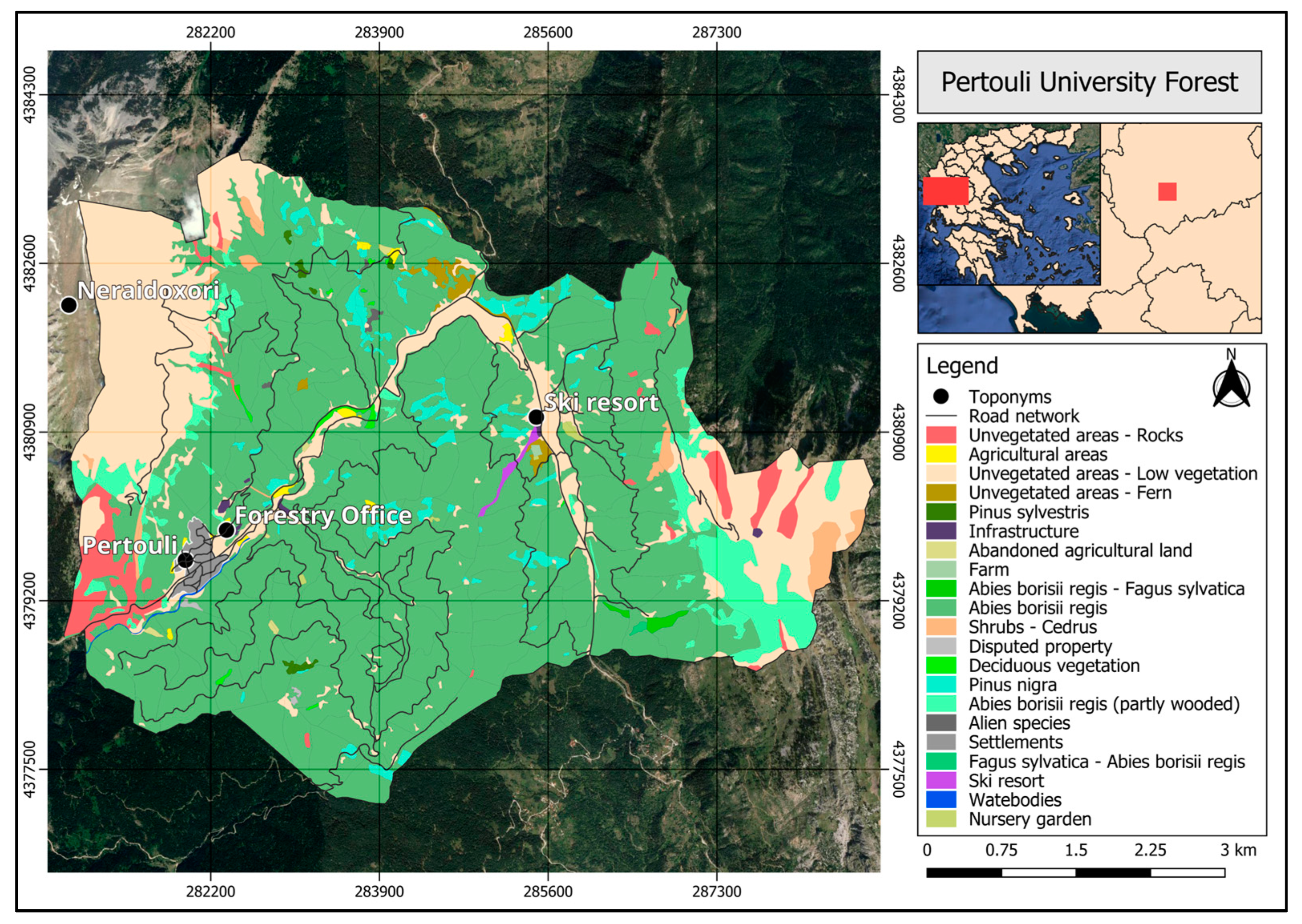
The study area is the Pertouli University Forest, located in the Pindos Mountain Range of Central Greece (latitude 39°32′–39°35′ and longitude 21°33′–21°38′) (Figure 1). The forest is managed by the Aristotle University of Thessaloniki and serves research and educational activities. The altitude of the area ranges between 1100 m and 2073 m above mean sea level, and the climate is characterized as transitional, Mediterranean-Mid-European (i.e., rainy, cold winters and dry, warm summers). The forest occupies an area of 3296.59 ha, most of which (i.e., 2427.62 ha) is covered with pure natural hybrid Abies borisii regis (Abies alba Mill. X Abies cephalonica Loud.) stands. This species forms a tall, coniferous, uneven-aged structured forest with a dense understory due to its shade-tolerant properties. A total of 130.74 ha of the remaining area is covered by non-vegetated areas within the forest, 555.40 ha by mountain pastures, 114 ha by lowland grasslands, and 68.83 ha are occupied by agricultural areas and settlements.
2.2. Dataset Description
2.2.1. Airborne LiDAR Data
The remote sensing data employed in the present study are composed of ALS-derived point clouds covering the entire area of the Pertouli University Forest. In particular, the ALS data were acquired in October of 2018 using a RIEGL VQ-1560i-DW laser scanner (RIEGL Laser Measurement Systems GmbH, Riedenburgstraße 48, A-3580 Horn, Austria) mounted on an airplane at an average altitude of 2243 m above the terrain. The point cloud is characterized by a very high point density (i.e., approximately 83 points/m2), a pulse spacing of 0.13 m, and a ground-to-total returns percentage of 27% (i.e., 24 points/m2). In addition, aerial photographs were acquired using a Phase One IXU_1000RS (Copenhagen, Denmark) with a Rodenstock 50 mm (Munich, Germany) sensing (i.e., a spatial resolution of 10 cm) simultaneously with the ALS data over the entire study area.
2.2.2. Ground Inventory Data
The in situ data were collected in October 2019 by measuring specific variables of individual fir trees, including the diameter at breast height (DBH), the tree height, and the crown radius. In particular, the DBH of each tree was measured using a Haglof Mantax Blue caliper, while the measurements of the tree heights included the use of a Blume–Leiss altimeter. Given the precision (i.e., 0.5 m) of the Blume–Leiss altimeter and potential measurement errors of random nature (e.g., leaning trees or branches obscurement due to dense canopy), the tree height was measured at least three times for each tree, and the average value was set as reference [28]. The crown radius was recorded using a laser distance meter (i.e., Leica Disto D2) through the radius measurement across the four main axes of each tree. The final crown radius for each individual tree was calculated using the arithmetic mean of all four measured radii. As a result, a total of 300 trees were registered, and their data were homogenized for further analysis. It is worth mentioning that the selected trees were representative samples characterized by different social statuses and attributes. The aforementioned field data were used to apply the methodology described in Section 2.3.
Additionally, positional measurements were conducted during the same time period in 38 sample plots of 1000 sq. m. each (rectangle 40 m × 25 m) covered by pure dense Abies borisii regis stands. In particular, the locations of the plots’ corners were recorded using a handheld GNSS with an average horizontal positional accuracy of 3 m. The specific plot dimensions are based on the sampling method applied for managing the forest, one of the two methods (fixed-area plots of size 40 m × 25 m or Bitterlich plots) employed for the forest management plans development in Greece. These plot measurements were used for the accuracy assessment of the generated products.
2.3. LiDAR Data Processing
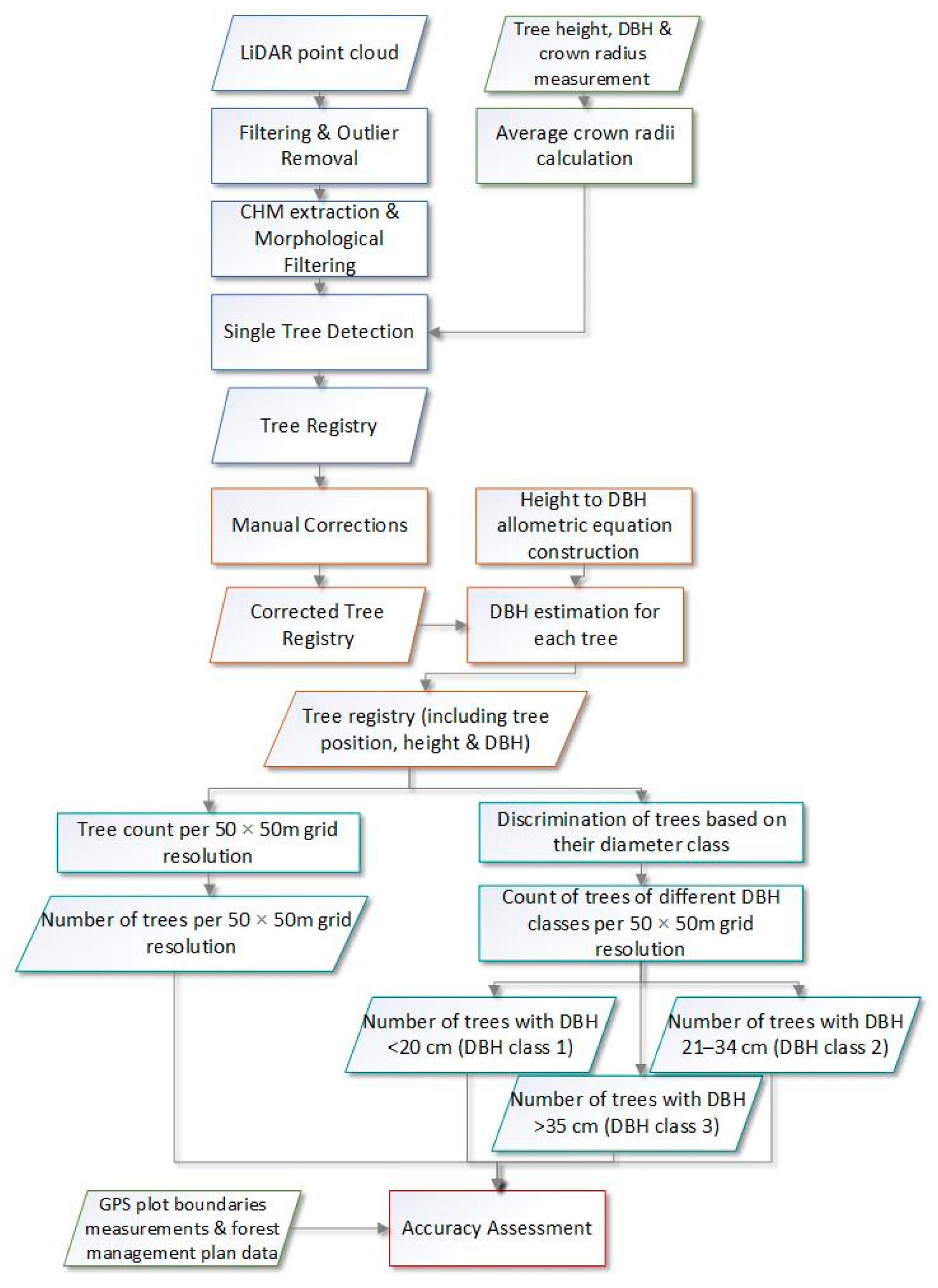
The methodology employed in the present study was composed of two processing parts. The first one includes the ALS data processing for the generation of a detailed tree registry for the entire study area, including the height and DBH information for each individual tree, as well as four tree density maps at 50 m resolution, providing the number of all trees and the number of trees characterized by three different DBH classes (i.e., class 1: ≤20 cm, class 2: 21–34 cm, and class 3: ≥35 cm). In accordance with common forest practice, the information provided by the aforementioned products is essential for conducting all activities related to cut-tree marking [29].
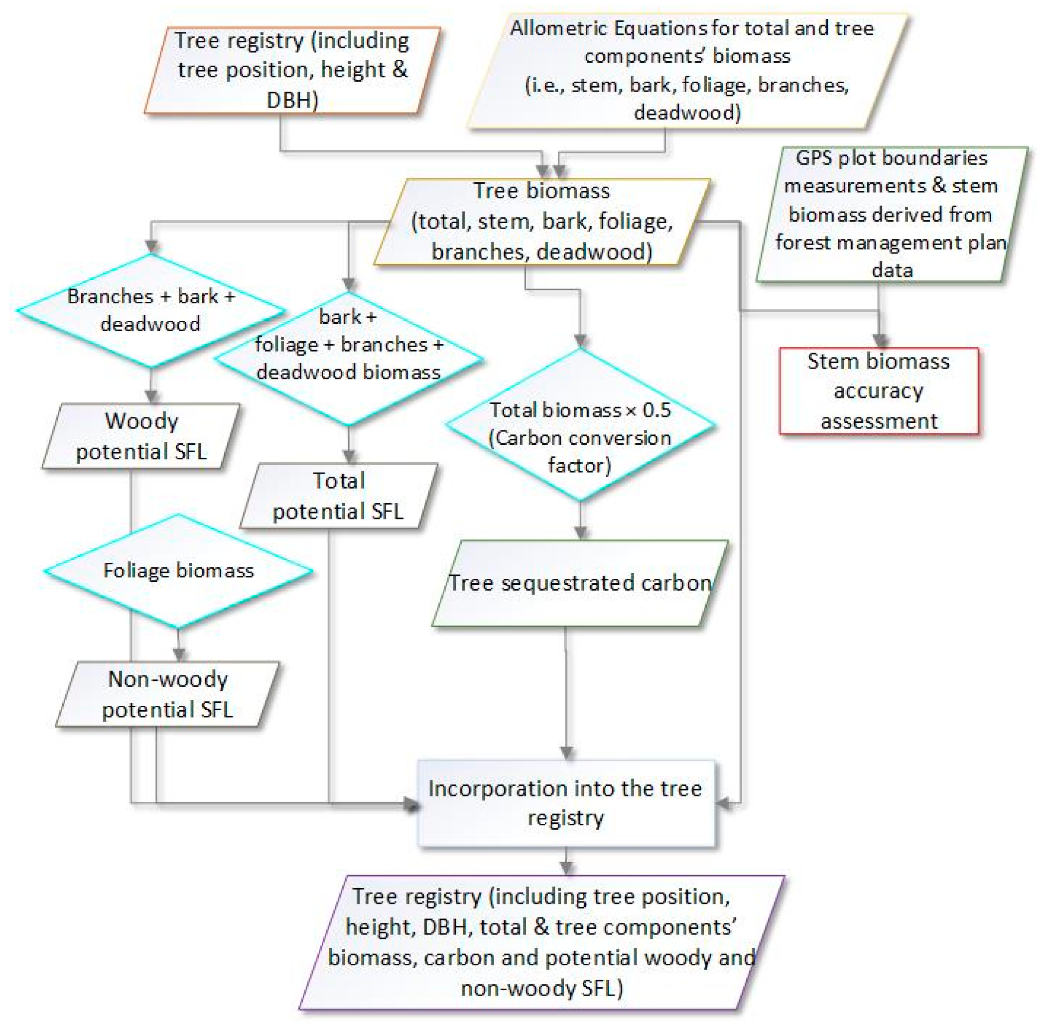
The second part of the employed methodology refers to estimating additional tree parameters using the information provided by the tree registry (i.e., tree height and DBH). These tree parameters include the total stem, bark, foliage, branches, and deadwood tree biomass, the sequestrated carbon, and the total woody and non-woody potential SFL. The estimated information is essential for forest and fire managers to evaluate carbon and SFL-related ecological impacts after each harvesting activity.
The workflow of the entire methodology is presented in the following flowcharts (Figure 2 and Figure 3).
2.3.1. Tree Registry Generation
The ALS point cloud was initially filtered for noise removal with the statistical outliers removal algorithm using the default parameters [30]. According to this method, points having more than three times the standard deviation of the cloud’s average distance were removed [31]. The points of the filtered cloud were labeled as ground and non-ground using the cloth simulation algorithm [32]. Subsequently, the ground points were interpolated using the k-nearest neighbor approach with an inverse distance weighting, constructing the digital terrain model (DTM) [33]. The produced DTM was eventually used to eliminate the terrain effects, resulting in a height-normalized point cloud.
The canopy height model (CHM) was generated using the pit-free algorithm, significantly improving the tree detection accuracy in high- and low-density ALS point clouds [34]. In addition, morphological erosion with a cross-shaped structuring element was applied to enhance the severability of all trees due to the complex canopy structure. The resolution of both rasters (i.e., DTM and CHM) was set to 0.5 m, which was defined based on the nominal point spacing of the ALS data [35].
Although a handful of methods have been developed for tree detection [15,36,37,38,39], most studies rely on local maxima detection of CHM. More specifically, a moving window is used to determine the positions and height of the detected trees based on the local maxima filter. The window size was set to 5.75 m, two times the average crown radius measured in the field. Each tree’s position (i.e., X, Y coordinates and altitude) and height were stored, while the detected tree tops below three meters in height were removed from the produced tree registry.
2.3.2. Tree Registry Evaluation and Manual Correction
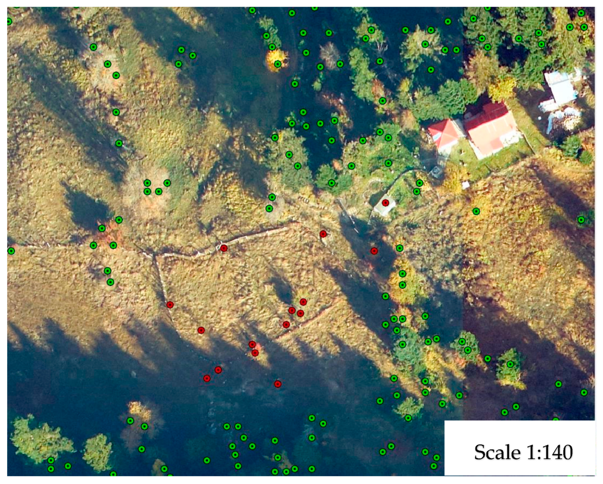
Following the generation of the tree registry for the entire Pertouli University Forest, the product was visually inspected and manually corrected wherever required. In particular, aerial photographs of very high spatial resolution (i.e., 10 cm), acquired simultaneously with the ALS point cloud, were employed to inspect the developed tree registry and its’ modification. The detected errors originated from the presence of rocks, buildings, pillars, cables, and other artificial surfaces, wrongly considered trees by the employed tree detection algorithm. Therefore, the points (i.e., tree tops) generated over the aforementioned areas were removed from the tree registry. Figure 4 illustrates a typical example of an area where several points were wrongly created over artificial surfaces and subsequently removed for the generation of the final product.
Finally, the corrected tree registry was subset to the boundaries of the Abies borisii regis-covered area.
2.3.3. Height to DBH Conversion Equation
The next processing step included the incorporation of the DBH into the produced tree registry, which constitutes one of the most vital pieces of information to be provided to the local forest managers during the cut-tree marking period. Given the limited ability of ALS to detect stems and provide direct DBH measurements, a log-transformed linear model was developed (Equation (1)) to derive the DBH from each detected tree, using the tree height and DBH data collected on the field.
where DBH is the diameter at the breast height of each tree, and are the intercept and scaling coefficient, respectively, and is the residual error.
The constructed allometric equation was applied to each tree included in the developed tree registry using the already incorporated tree height information. The resulting DBH was finally integrated into the tree registry to generate the final product. The prediction performance of the constructed allometric equation was evaluated based on the relative square error (RSE), R2, and adjusted R2 (adjR2).
2.3.4. Estimation of Tree Parameters
A set of allometric equations, developed by Georgopoulos et al. [22,24], was employed to calculate total and tree components’ biomass. The aforementioned equations were specifically developed for fir species, using each tree’s DBH and height to estimate each individual’s stem, bark, branches, and needles biomass. Although tree volume is identified as the main decision factor for cut-tree marking activities, biomass, and sequestered carbon are considered the most important parameters in sustainable and adaptive forest management [40]. Therefore, a series of biomass and carbon-related parameters (i.e., sequestered carbon, potential SFL, potential woody SFL, and potential non-woody SFL) was estimated for each tree, providing valuable information about the carbon stock emissions and the ecological impact of the harvesting activities in the ecosystem.
The total SFL represents the full weight of the harvesting residues that will potentially remain in the forest, and it is estimated as the sum of all biomass components except the stem. In addition, the SFL was further discriminated into woody and non-woody, referring to the woody biomass components (bark, branches, deadwood) and foliage, respectively. Finally, the sequestered carbon for each tree was calculated by multiplying the total aboveground biomass by the carbon conversion factor (i.e., 0.5).
2.3.5. Tree Density Maps Generation
The last part of the analysis process included the generation of four tree-density products, which provided additional necessary information to the forest manager and field worker during cut-tree marking. Initially, the number of trees was calculated per 50 m × 50 m grid resolution using the developed tree registry, leading to the generation of the general tree density map. Next, the calculation of the number of trees was performed using the DBH information included in the registry. As a result, three additional products were produced, each of which included the number of trees belonging to one of the three DBH classes (i.e., class 1: <20 cm, class 2: 21–34 cm, and class 3: >35 cm) on a 50 m × 50 m grid resolution.
2.3.6. Accuracy Assessment
Quantitative accuracy assessment was performed for all four tree density maps and the stem biomass estimations, derived from the tree registry information (i.e., height and DBH) and applying an existing allometric equation [24]. On the contrary, since the tree registry product was thoroughly examined and manually corrected, its validation was not considered necessary at this point.
The reference data employed for the accuracy evaluation of the general tree density map include the GPS measurements of the 38 plot boundaries (as described in Section 2.2.2) as well as the forest management plan for the year 2018. Each plot’s boundaries were used to delineate the respective boundaries on the tree registry. Next, the number of trees in total and per DBH class was calculated based on the tree tops included within each delineated plot. The resulting tree number and the estimated stem biomass per tree were compared with the respective parameters provided by the forest management plan.
In particular, three standard goodness-of-fit metrics were calculated for the quantitative assessment of the products’ performance, namely the coefficient of determination (R2) (Equation (2)), the adjusted coefficient of determination (Adj.R2) (Equation (3)) and the relative squared error (RSE) (Equation (4)).
where is the observed value for plot , is the estimated value for plot , is the mean observed value, and is the number of plots.
3. Results
In the present work, we employed ALS data covering a dense, uneven-aged structured, coniferous forest to generate products essential for operational cut-tree marking activities to actively support long-term sustainable forest management. Specifically, five products were generated in accordance with the needs of the local forest managers responsible for the related field work in our study area. The products include a tree registry of the forest covered by the Abies borisii regis species, a tree density map of a 50 m resolution as well as three additional density maps illustrating the number of trees of the individual DBH classes (i.e., class 1: ≤20 cm, class 2: 21–34 cm, and class 3: ≥35 cm) on a 50 m × 50 m grid resolution. Finally, we propose a workflow (described in detail in Section 4) for practically employing the generated products during and post-cut-tree marking activities.
3.1. Height to DBH Allometric Equation
3.2. Tree Registry and Tree Density Maps
The products derived from the ALS data analysis are presented in Figure 5, Figure 6, Figure 7, Figure 8 and Figure 9. The produced tree registry was initially composed of 882,771 individuals, including all forest species. However, since selective tree logging in our study area is performed only on the Abies borisii regis species, the points representing the tops of other tree species, such as black and Scots pine (Pinus nigra and Pinus silvestris) and beech (Fagus moesiaca), were removed from the initial tree registry. In total, 94,554 points were removed, resulting in the generation of a tree registry composed of 789,816 fir tops (Figure 5). The tree height included in the registry ranges from 3 to 35 m.
Except for the height and DBH information incorporated into the tree registry, ten additional tree parameters were estimated, namely the stem, deadwood, needles, branches, bark and total aboveground biomass, sequestered carbon, potential total, and woody and non-woody SFL derived from the harvesting procedures (Table 2). These parameters are essential for the adaptive management of forest ecosystems, providing accurate quantification of the harvest residues and carbon losses.
The general tree density map is illustrated in Figure 6, providing information on the number of trees per a 2500 sq. m. area. The minimum number of trees in the fir-covered forest is one, and the respective maximum value is 174. The areas of low tree density are mainly located at the forest boundaries as well as within the surroundings of the road network. On the contrary, the densest forest stands can be found at the higher parts of the forest, namely above the altitude of 1200 m.
The three remaining tree density products are depicted in Figure 7, Figure 8 and Figure 9, presenting the number of trees within 2500 sq. m. of the three DBH classes, respectively. Specifically, the results show that trees with a DBH of class 1 (i.e., ≤20 cm.) are mostly located at high altitudes in the Eastern and Western parts of the forest (Figure 6). Trees with a DBH of class 2 (i.e., 21–34 cm.) mostly cover the southern part of the forest, while trees of class 3 DBH (≥35 cm.) can be almost equally found throughout the entire area.
3.3. Accuracy Assessment Results
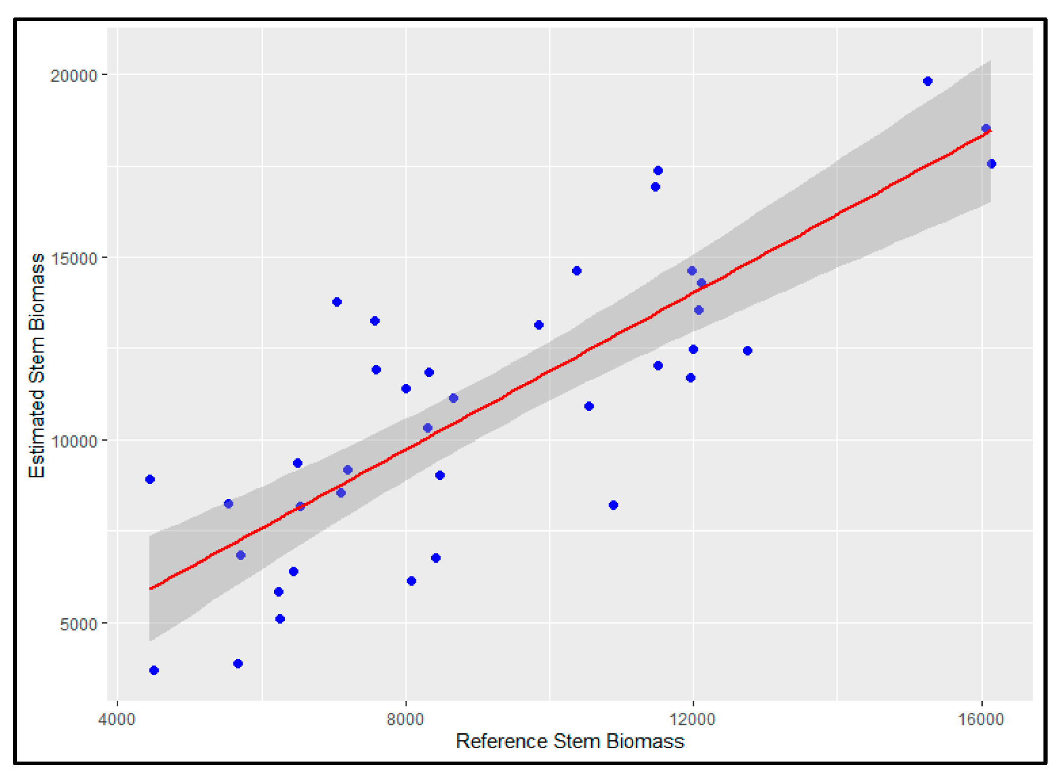
Table 3 presents the results of the accuracy assessment process performed for the four tree density maps and the stem biomass estimated using the height, and the DBH provided using the produced tree registry. More specifically, the R2, AdjR2, and RSE for the general tree density map were calculated to be 0.14, 0.12, and 5.72, respectively. Furthermore, the goodness-of-fit statistics showcase R2 values ranging from 0.15 to 0.61 for the tree density maps referring to the three different DBH classes (i.e., class 1: ≤20 cm, class 2: 21–34 cm, and class 3: ≥35 cm). In particular, the R2 and Adj. R2 have been calculated to be 0.15 and 0.12, 0.20 and 0.18, and 0.61 and 0.60 for DBH classes 1, 2, and 3, respectively, while the RSE reached 5.09 for DBH class 1, 5.21 for DBH class 2, and 5.15 for DBH class 3. As for the accuracy of the estimated stem biomass, the employed allometric equation achieved an R2 value of 0.67, an AdjR2 of 0.66, and an RSE of 1813.
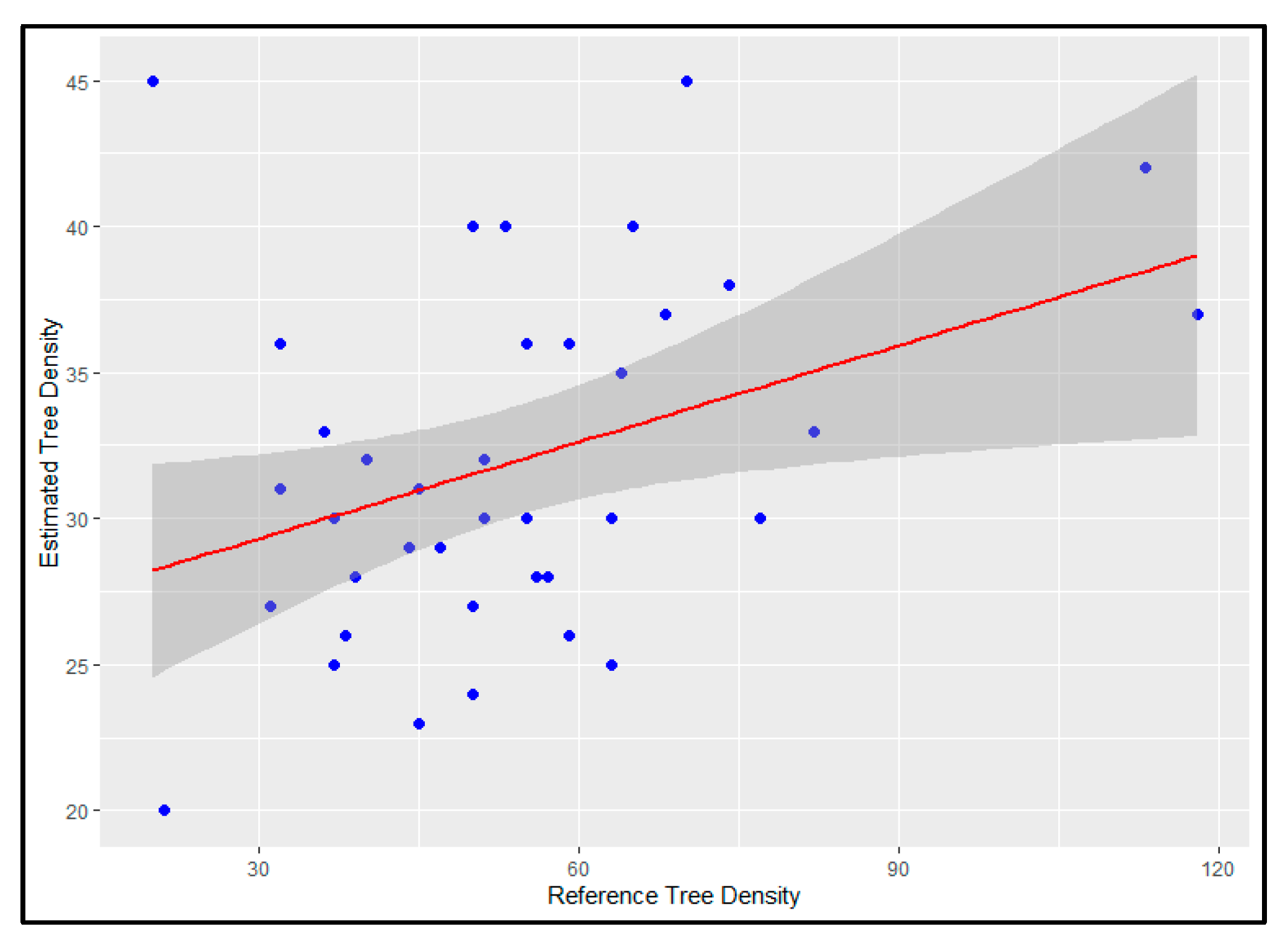
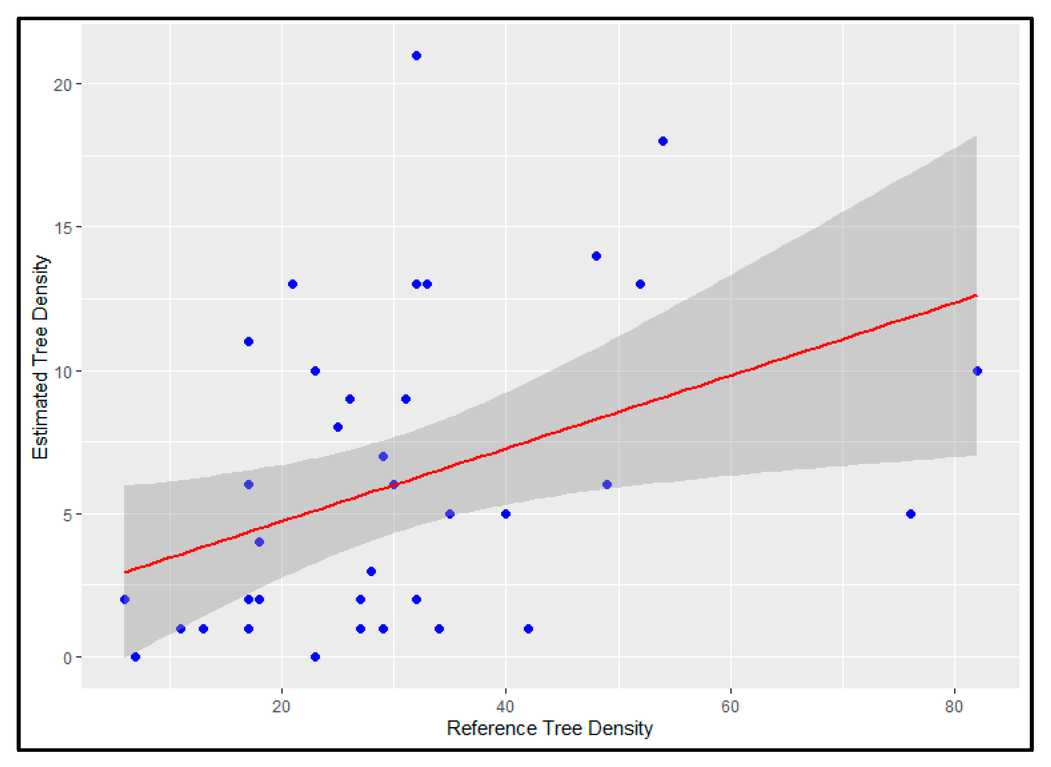
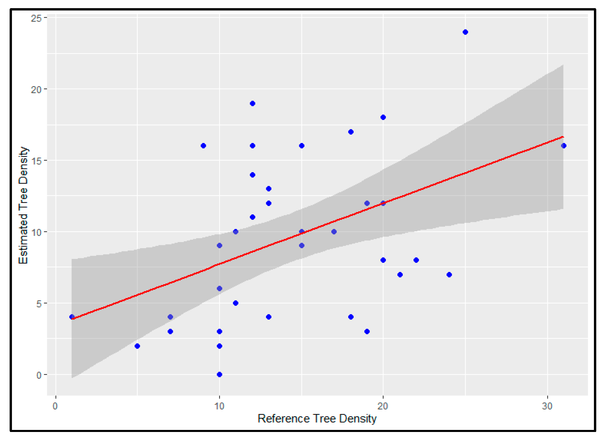
Further examination of the aforementioned results (Table 2) can also be performed through the reference versus estimated values depicted in Figure 10, Figure 11, Figure 12, Figure 13 and Figure 14. The scatterplots presented in Figure 10, Figure 11 and Figure 12 showcase that the tree density (i.e., number of trees) most accurately estimated (R2 = 0.61) is the one including the trees of DBH class 3 (i.e., ≥35 cm), while the general tree density map and the one including trees of DBH class 1 are characterized by the highest estimation error (R2 = 0.14 and R2 = 0.15, respectively). The satisfying estimation accuracy of the tree stem biomass (R2 = 0.67) is also illustrated in the respective scatterplot (Figure 14), which shows no significant over and underestimation errors.
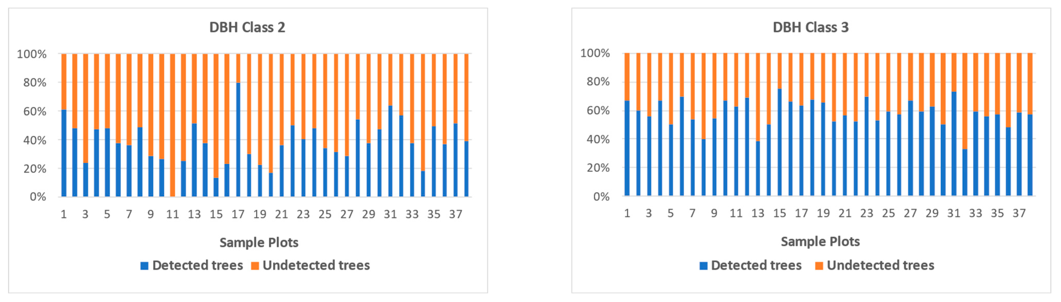
Finally, for the sake of comprehensible results presentation, the percentage of detected and undetected trees in each sample is illustrated in the following stacked bar graphs (Figure 15). The comparison of the graphs confirms the aforementioned results related to the accuracy of the tree density maps.
4. Discussion
A series of ALS-derived products were generated in this work to be employed by forest managers and/or field workers and facilitate the yearly operational cut-tree marking activities within our study area (i.e., Pertouli University Forest). Considering the forest managers’ needs and according to common forest practice, we also propose a workflow for the practical employment of the results during and post-cut-tree marking activities. This study constitutes among the first known applications of ALS data for developing a tree registry covering an entire forest to be applied in the context of operational tree-marking and long-term sustainable forest management.
The LiDAR analysis performed to produce the tree registry and density maps (Figure 4, Figure 5, Figure 6, Figure 7 and Figure 8) were based on the most widely and successfully employed techniques. In fact, the very high point cloud density allowed the implementation of some of the well-established processing algorithms, such as point cloud classification, cloth simulation, and local maxima filter, ensuring the highest possible validity of the resulting products [25,39,41]. The results were assessed for their accuracy using data collected on the field.
The tree detection errors created in the registry product were visually identified. These errors can be attributed to the complex multi-layered structure of the forest [15] and were manually corrected through photo interpretation of the very high-resolution aerial imagery acquired along with the ALS point cloud data. The manual correction, although time-consuming, was the only direct method for the accuracy of the tree registry to reach the highest level possible.
The accuracy assessment of the tree density maps was performed with the use of field data. The results (Table 1 and Figure 10, Figure 11, Figure 12 and Figure 13) indicate that as the trees’ DBH increases, the tree detection algorithm’s performance also increases. More specifically, trees characterized by DBH ≤ 20 cm (i.e., DBH class 1) mostly belong to the understory vegetation since Abies borisii regis constitutes a shade-tolerant species. This means that these trees frequently remain undetected by the LiDAR sensor. Nevertheless, despite the low accuracy of the product, it provides valuable information for cut-tree marking. In fact, the higher number of detected DBH class 1 trees indicates the higher detection capability of the LiDAR sensor, which can be attributed to the fact that the examined area is not covered by dense overstory. As such, it can be confidently assumed that the area is covered by natural regeneration and, considering that falling trees can severely damage it, such areas are not considered suitable for harvest. Therefore, the information provided by the respective tree density map can be ancillary used during the process of cut-tree marking for the proper selection of the harvesting area. With regard to the trees with DBH from 21 to 34 cm (i.e., class 2) (co-dominant trees), they present intense competition with the ones of DBH ≥ 35 cm (i.e., class 3) (dominant tree). Hence, similar to the DBH class1 trees, the co-dominant trees are usually located underneath the canopy of the dominant ones and are difficult to identify using the LiDAR sensor. In summary, trees of DBH classes 1 and 2 often remain undetected due to the unevenly aged structure of the forest, which led to the low accuracy of the respective tree density maps.
Contrary to the DBH classes 1 and 2, the dominant trees were accurately detected from the ALS point cloud, which is depicted both by the goodness-of-fit statistics (Table 1) and the comparison scatterplot (Figure 13). In fact, this product provides the most significant information for cut-tree marking since dominant trees of high commercial value are mostly selected for harvesting in the framework of economic-oriented management. Finally, as expected, the general tree density map incorporates the accuracy of all three aforementioned density maps, which results in an R2 of 0.61 compared with the reference data.
Despite the inability of ALS technology to detect each and every tree in a multi-layered forest and complex terrain, which resulted in the low accuracy of some of the generated products, we endeavored their full and efficient exploitability within the framework of operational cut-tree marking and long-term sustainable forest management. In particular, we propose a workflow methodology that focuses on the appropriate use of the products so that each fieldwork is completed promptly and efficiently.
More specifically, the forest manager is recommended to use a GIS mobile application, which can serve as a complementary tool for forest management since it enables faster and more accurate (compared to the use of study) field data collection, reliable data analysis, and an efficient real-time update of the collected sddata whenever required [40,42]. For decades, researchers have been developing mobile GIS applications for a variety of environmental field surveys, including forest tree measurements [42,43,44,45,46]. Nowadays, a number of mobile GIS applications exist, either open-source or proprietary, such as QField (https://qfield.org/, accessed on 1 October 2023), ArcGIS Field Maps (https://www.esri.com/en-us/arcgis/products/arcgis-field-maps/overview, accessed on 1 October 2023), and ArcGIS Survey123 (https://survey123.arcgis.com/, accessed on 1 October 2023), which provide users with all the aforementioned possibilities during fieldwork.
Prior to fieldwork and based on the information provided by the forest management plan, a specific forest compartment (the respective map is provided in the context of the forest management plan) is defined as the area suitable for harvesting. Next, the manager is required to consult the forest management plan about the amount of timber volume (i.e., the number of trees and their specific DBH class/classes) that needs to be deducted from the selected forest compartment. Based on this information, the areas with the highest tree density of the DBH class/classes of interest should be located using the DBH-related tree density maps (Figure 7, Figure 8 and Figure 9). Based on the general tree density map (Figure 6) and expert knowledge, the manager can then locate the sub-areas characterized by a sufficient tree density, ensuring that the scheduled harvesting will not impact the forest’s sustainability. Next, the field worker will use the ALS-derived tree registry (Figure 5) to select the trees suitable for harvest on the site based on their geographical position, height, and visual assessment. The completion of the harvesting process can be followed by the update of the tree registry by removing the points that represent the tops of the deducted trees. Moreover, the additionally estimated tree parameters, i.e., the total and the tree components’ (stem, foliage, branches, bark, and deadwood) biomass, the tree sequestrated carbon, and the potential total, woody, and non-woody SFL can serve as a basis for the assessment of the post-harvesting carbon and potential SFL-related ecological impacts. Finally, except for the cut-tree marking process, the tree registry product can be used in a variety of forest applications, such as diseases and potential risk records.
Following the above-described cut-tree marking methodology, the expert is directly provided with the necessary knowledge about tree distribution and characteristics using the ALS-derived spatial layers. The proposed methodology also enables the quick and accurate definition of the area suitable for harvesting and, thus, ensures the reduced required man effort compared to the traditional method of cut-tree marking. In fact, following the selection of the area densely covered by the trees of interest, the field worker can identify the location of the trees of interest within the 2500 sq. m. area through access to all the necessary information about the essential characteristics (i.e., DBH and height) of each tree using the tree registry product. Moreover, the forest manager and the field worker are provided with the possibility of a straightforward digital update of the forest tree registry after the performed harvesting. As such, the products generated within the context of this work and the employed GIS technology can support sustainable forest management for a long-term time period. Overall, the proposed methodology can be applied to any other forest where selective harvesting is being performed in its management framework.
Nevertheless, although the present study has reached its aim, some unavoidable limitations exist. Specifically, the high density of the forest canopy can cause errors in the GPS measurement made by the marker. However, these errors can be manually corrected through the employed GIS mobile app. Although the development of the proposed methodology was based on the current specific needs of the local forest managers and field workers, no tree-marking activities have yet been performed in the Pertouli University Forest. Additionally, the presented results are experimental, and all findings are intended for research purposes in the current state. Therefore, if needed, the methodology will be applied, evaluated, and adjusted during the next scheduled marking period (i.e., spring 2024).
Finally, it is worth noting that, except for the cut-tree marking activities, the tree registry developed within the context of the present study can be employed in various applications related to the forest’s sustainable management. More specifically, this ALS-derived product can be utilized for the detailed record of diseases per individual tree and for other potential risks/disasters related to biotic and abiotic factors. Last but not least, the tree registry can serve for the prediction and post-harvesting estimation of the forest’s carbon stock prior to and after harvesting, respectively, in the context of carbon-oriented management.
5. Conclusions
This study’s primary focus was examining the potential of ALS data in enhancing operational tree-marking activities in a dense coniferous forest characterized by an unevenly aged structure and intense terrain to actively support long-term sustainable forest management. A comprehensive tree registry and tree density maps were developed, covering the entire extent of the forest. In addition, a methodology was proposed, following standard forest practices, to effectively make use of the ALS-derived products during cut-tree marking activities. The aim was to streamline and optimize the process of conducting cut-tree marking activities, saving time and effort. It is worth mentioning that the developed ALS-derived tree registry constitutes among the first known that cover an entire forest area and aim at being employed in the context of operational sustainable forest management. More specifically, the conclusions that can be drawn from our study are the following:
- The tree registry was manually corrected, resulting in the highest possible accuracy of the product itself and its derivatives (i.e., tree density maps);
- The trees of DBH ≤ 20 cm (class 1) and DBH 21–34 cm (class 2) were not accurately detected due to the multi-layered structure of the forest. On the contrary, the DBH ≥ 35 cm trees were reliably identified since they are the dominant ones and fully detectable using the LiDAR sensor;
- Despite the LiDAR sensor’s low detection capability in areas with high tree density and small DBH classes, the map indicates the absence of co-dominant or dominant trees and the strong presence of regeneration. This provides the user with the ability to directly decide whether the respective area is considered suitable for harvest, as falling trees can severely damage regeneration trees during logging;
- The tree density map of DBH class 3 demonstrates high reliability, which is of utmost importance as this information is commonly used during cut-tree marking activities;
- Among the tree parameters that were additionally estimated and incorporated into the tree registry descriptive information, the stem biomass was assessed for its accuracy through its comparison with the respective data provided by the forest management plan (2018). The results showcased that the stem biomass was reliably estimated, presenting an R2 value of 0.67;
- Except for cut-tree marking and harvesting activities, all products generated within the context of this work can be employed for various other environmental management purposes, such as the development and adoption of climate mitigation and adaptation strategies, as well as monitoring biotic and abiotic components of forest ecosystems;
- Considering the common forest practice, the present work provides detailed guidelines for using the produced products (tree registry and tree density maps) to facilitate the process of selective cut-tree marking in terms of time and effort efficiency;
- The presented methods, results, and findings are experimental, and the methodology will be applied and evaluated during the next scheduled marking period by the University Forest Service (i.e., spring 2024).
Future research will involve the application of the developed methodology and the ALS-derived products in the field, their evaluation, and appropriate adjustment, if required, according to the forest manager’s needs. The ALS data employed in this study will also be examined for their potential to accurately delineate the crown of each individual tree over the entire forest. This will enable the accurate estimation of the forest gaps area created after the deduction of each tree, which can provide forest managers with valuable knowledge related to the natural regeneration and succession of the forest.
Author Contributions
Conceptualization, N.G. and I.Z.G.; methodology, N.G. and A.S.; software, N.G.; validation, N.G. and I.Z.G.; formal analysis, N.G.; investigation, N.G. and A.S.; resources, I.Z.G.; data curation, N.G. and A.S.; writing—original draft preparation, A.S.; writing—review and editing, N.G., A.S. and I.Z.G.; visualization, N.G. and A.S.; supervision, I.Z.G.; project administration, I.Z.G.; funding acquisition, I.Z.G. All authors have read and agreed to the published version of the manuscript.
Funding
This study was funded by the University Forest Administration and Management Fund of the Aristotle University of Thessaloniki (Greece) within the context of the project “Exploitation of LiDAR data for the production of forest parameters to support forest management at local level” (98730). Airborne LiDAR data acquisition was also funded by the University Forest Administration and Management Fund of the Aristotle University of Thessaloniki (Greece) (http://uniforest.auth.gr/, accessed on 22 November 2023).
Data Availability Statement
No new data were created or analyzed in this study. Data sharing is not applicable to this article.
Conflicts of Interest
The authors declare no conflict of interest. The funders had no role in the design of the study, in the collection, analyses, or interpretation of data, in the writing of the manuscript, nor in the decision to publish the results.
References
- Nunes, L.J.R.; Meireles, C.I.R.; Pinto Gomes, C.J.; Almeida Ribeiro, N.M.C. Forest Management and Climate Change Mitigation: A Review on Carbon Cycle Flow Models for the Sustainability of Resources. Sustainability 2019, 11, 5276. [Google Scholar] [CrossRef]
- Ma, W.; Zhou, X.; Liang, J.; Zhou, M. Coastal Alaska Forests under Climate Change: What to Expect? For. Ecol. Manag. 2019, 448, 432–444. [Google Scholar] [CrossRef]
- Pörtner, H.-O.; Roberts, D.C.; Adams, H.; Adler, C.; Aldunce, P.; Ali, E.; Begum, R.A.; Betts, R.; Kerr, R.B.; Biesbroek, R. Climate Change 2022: Impacts, Adaptation and Vulnerability; IPCC: Geneva, Switzerland, 2022. [Google Scholar]
- Harris, N.L.; Gibbs, D.A.; Baccini, A.; Birdsey, R.A.; De Bruin, S.; Farina, M.; Fatoyinbo, L.; Hansen, M.C.; Herold, M.; Houghton, R.A.; et al. Global Maps of Twenty-First Century Forest Carbon Fluxes. Nat. Clim. Chang. 2021, 11, 234–240. [Google Scholar] [CrossRef]
- Thomas, J.; Brunette, M.; Leblois, A. The Determinants of Adapting Forest Management Practices to Climate Change: Lessons from a Survey of French Private Forest Owners. For. Policy Econ. 2022, 135, 102662. [Google Scholar] [CrossRef]
- Latterini, F.; Stefanoni, W.; Venanzi, R.; Tocci, D.; Picchio, R. GIS-AHP Approach in Forest Logging Planning to Apply Sustainable Forest Operations. Forests 2022, 13, 484. [Google Scholar] [CrossRef]
- Pichler, G.; Poveda Lopez, J.A.; Picchi, G.; Nolan, E.; Kastner, M.; Stampfer, K.; Kühmaier, M. Comparison of Remote Sensing Based RFID and Standard tree Marking for Timber Harvesting. Comput. Electron. Agric. 2017, 140, 214–226. [Google Scholar] [CrossRef]
- Eberhard, B.; Hasenauer, H. Tree Marking versus Tree Selection by Harvester Operator: Are There Any Differences in the Development of Thinned Norway Spruce Forests? Int. J. For. Eng. 2021, 32, 42–52. [Google Scholar] [CrossRef]
- Rainey, J. Digital Technology Enhances Tree Marking Effectiveness in Meeting Restoration Objectives in Southwestern Ponderosa Pine. Ph.D. Thesis, Northern Arizona University, Flagstaff, AZ, USA, 2021. [Google Scholar]
- Zianis, D.; Xanthopoulos, G.; Kalabokidis, K.; Kazakis, G.; Ghosn, D.; Roussou, O. Allometric Equations for Aboveground Biomass Estimation by Size Class for Pinus Brutia Ten. Trees Growing in North and South Aegean Islands, Greece. Eur. J. For. Res. 2011, 130, 145–160. [Google Scholar] [CrossRef]
- Saukkola, A.; Melkas, T.; Riekki, K.; Sirparanta, S.; Peuhkurinen, J.; Holopainen, M.; Hyyppä, J.; Vastaranta, M. Predicting Forest Inventory Attributes Using Airborne Laser Scanning, Aerial Imagery, and Harvester Data. Remote Sens. 2019, 11, 797. [Google Scholar] [CrossRef]
- Latifi, H.; Heurich, M. Multi-Scale Remote Sensing-Assisted Forest Inventory: A Glimpse of the State-of-the-Art and Future Prospects. Remote Sens. 2019, 11, 1260. [Google Scholar] [CrossRef]
- Hamedianfar, A.; Mohamedou, C.; Kangas, A.; Vauhkonen, J. Deep Learning for Forest Inventory and Planning: A Critical Review on the Remote Sensing Approaches so far and Prospects for Further Applications. For. Int. J. For. Res. 2022, 95, 451–465. [Google Scholar] [CrossRef]
- Latella, M.; Sola, F.; Camporeale, C. A Density-Based Algorithm for the Detection of Individual Trees from LiDAR Data. Remote Sens. 2021, 13, 322. [Google Scholar] [CrossRef]
- Eysn, L.; Hollaus, M.; Lindberg, E.; Berger, F.; Monnet, J.-M.; Dalponte, M.; Kobal, M.; Pellegrini, M.; Lingua, E.; Mongus, D.; et al. A Benchmark of Lidar-Based Single Tree Detection Methods Using Heterogeneous Forest Data from the Alpine Space. Forests 2015, 6, 1721–1747. [Google Scholar] [CrossRef]
- Wang, X.-H.; Zhang, Y.-Z.; Xu, M.-M. A Multi-Threshold Segmentation for Tree-Level Parameter Extraction in a Deciduous Forest Using Small-Footprint Airborne LiDAR Data. Remote Sens. 2019, 11, 2109. [Google Scholar] [CrossRef]
- Dai, W.; Yang, B.; Dong, Z.; Shaker, A. A New Method for 3D Individual Tree Extraction Using Multispectral Airborne LiDAR Point Clouds. ISPRS J. Photogramm. Remote Sens. 2018, 144, 400–411. [Google Scholar] [CrossRef]
- Li, W.; Guo, Q.; Jakubowski, M.K.; Kelly, M. A New Method for Segmenting Individual Trees from the Lidar Point Cloud. Photogramm. Eng. Remote Sens. 2012, 78, 75–84. [Google Scholar] [CrossRef]
- Kaartinen, H.; Hyyppä, J.; Yu, X.; Vastaranta, M.; Hyyppä, H.; Kukko, A.; Holopainen, M.; Heipke, C.; Hirschmugl, M.; Morsdorf, F.; et al. An International Comparison of Individual Tree Detection and Extraction Using Airborne Laser Scanning. Remote Sens. 2012, 4, 950–974. [Google Scholar] [CrossRef]
- Goldbergs, G.; Maier, S.; Levick, S.; Edwards, A. Efficiency of Individual Tree Detection Approaches Based on Light-Weight and Low-Cost UAS Imagery in Australian Savannas. Remote Sens. 2018, 10, 161. [Google Scholar] [CrossRef]
- Kandare, K.; Ørka, H.O.; Chan, J.C.-W.; Dalponte, M. Effects of Forest Structure and Airborne Laser Scanning Point Cloud Density on 3D Delineation of Individual Tree Crowns. Eur. J. Remote Sens. 2016, 49, 337–359. [Google Scholar] [CrossRef]
- Georgopoulos, N.; Gitas, I.Z.; Korhonen, L.; Antoniadis, K.; Stefanidou, A. Estimating Crown Biomass in a Multilayered Fir Forest Using Airborne LiDAR Data. Remote Sens. 2023, 15, 2919. [Google Scholar] [CrossRef]
- Vauhkonen, J.; Ene, L.; Gupta, S.; Heinzel, J.; Holmgren, J.; Pitkänen, J.; Solberg, S.; Wang, Y.; Weinacker, H.; Hauglin, K.M.; et al. Comparative Testing of Single-Tree Detection Algorithms Under Different Types of Forest. For. Int. J. For. Res. 2012, 85, 27–40. [Google Scholar] [CrossRef]
- Georgopoulos, N.; Gitas, I.Z.; Stefanidou, A.; Korhonen, L.; Stavrakoudis, D. Estimation of Individual Tree Stem Biomass in an Uneven-Aged Structured Coniferous Forest Using Multispectral LiDAR Data. Remote Sens. 2021, 13, 4827. [Google Scholar] [CrossRef]
- Leite, R.V.; Amaral, C.H.D.; Pires, R.D.P.; Silva, C.A.; Soares, C.P.B.; Macedo, R.P.; Silva, A.A.L.D.; Broadbent, E.N.; Mohan, M.; Leite, H.G. Estimating Stem Volume in Eucalyptus Plantations Using Airborne LiDAR: A Comparison of Area- and Individual Tree-Based Approaches. Remote Sens. 2020, 12, 1513. [Google Scholar] [CrossRef]
- Contreras, M.A.; Parsons, R.A.; Chung, W. Modeling Tree-Level Fuel Connectivity to Evaluate the Effectiveness of Thinning Treatments for Reducing Crown Fire Potential. For. Ecol. Manag. 2012, 264, 134–149. [Google Scholar] [CrossRef]
- Contreras, M.A.; Chung, W. Developing a Computerized Approach for Optimizing Individual Tree Removal to Efficiently Reduce Crown Fire Potential. For. Ecol. Manag. 2013, 289, 219–233. [Google Scholar] [CrossRef]
- Yan, F.; Ullah, M.R.; Gong, Y.; Feng, Z.; Chowdury, Y.; Wu, L. Use of a No Prism Total Station for Field Measurements in Pinus Tabulaeformis Carr. Stands in China. Biosyst. Eng. 2012, 113, 259–265. [Google Scholar] [CrossRef]
- Pommerening, A.; Pallarés Ramos, C.; Kędziora, W.; Haufe, J.; Stoyan, D. Rating Experiments in Forestry: How Much Agreement Is There in Tree Marking? PLoS ONE 2018, 13, e0194747. [Google Scholar] [CrossRef]
- Carrilho, A.C.; Galo, M.; Santos, R.C. Statistical Outlier Detection Method for Airborne Lidar Data. Int. Arch. Photogramm. Remote Sens. Spat. Inf. Sci. 2018, XLII–1, 87–92. [Google Scholar] [CrossRef]
- Campbell, M.J.; Eastburn, J.F.; Mistick, K.A.; Smith, A.M.; Stovall, A.E.L. Mapping Individual Tree and Plot-Level Biomass Using Airborne and Mobile Lidar in Piñon-Juniper Woodlands. Int. J. Appl. Earth Obs. Geoinf. 2023, 118, 103232. [Google Scholar] [CrossRef]
- Zhang, W.; Qi, J.; Wan, P.; Wang, H.; Xie, D.; Wang, X.; Yan, G. An Easy-to-Use Airborne LiDAR Data Filtering Method Based on Cloth Simulation. Remote Sens. 2016, 8, 501. [Google Scholar] [CrossRef]
- Tu, J.; Yang, G.; Qi, P.; Ding, Z.; Mei, G. Comparative Investigation of Parallel Spatial Interpolation Algorithms for Building Large-Scale Digital Elevation Models. PeerJ Comput. Sci. 2020, 6, e263. [Google Scholar] [CrossRef] [PubMed]
- Khosravipour, A.; Skidmore, A.K.; Isenburg, M.; Wang, T.; Hussin, Y.A. Generating Pit-free Canopy Height Models from Airborne Lidar. Photogramm. Eng. Remote Sens. 2014, 80, 863–872. [Google Scholar] [CrossRef]
- Kodors, S. Point Distribution as True Quality of LiDAR Point Cloud. Balt. J. Mod. Comput. 2017, 5, 362–378. [Google Scholar] [CrossRef]
- Vega, C.; Hamrouni, A.; El Mokhtari, S.; Morel, J.; Bock, J.; Renaud, J.-P.; Bouvier, M.; Durrieu, S. PTrees: A Point-Based Approach to Forest Tree Extraction from Lidar Data. Int. J. Appl. Earth Obs. Geoinf. 2014, 33, 98–108. [Google Scholar] [CrossRef]
- Hu, X.; Chen, W.; Xu, W. Adaptive Mean Shift-Based Identification of Individual Trees Using Airborne LiDAR Data. Remote Sens. 2017, 9, 148. [Google Scholar] [CrossRef]
- Reitberger, J.; Schnörr, C.; Krzystek, P.; Stilla, U. 3D Segmentation of Single Trees Exploiting Full Waveform LIDAR Data. ISPRS J. Photogramm. Remote Sens. 2009, 64, 561–574. [Google Scholar] [CrossRef]
- Rutzinger, M.; Pratihast, A.K.; Elberink, S.J.O.; Vosselman, G. Detection and Modelling of 3D Trees from Mobile Laser Scanning Data. In Proceedings of the ISPRS Commission V Mid-Term Symposium, Close Range Image Measurement Techniques, Newcastle, UK, 21–24 June 2010; pp. 520–525. [Google Scholar]
- Jeefoo, P. Wildfire Field Survey using Mobile GIS Technology in Nan Province. In Proceedings of the 2019 Joint International Conference on Digital Arts, Media and Technology with ECTI Northern Section Conference on Electrical, Electronics, Computer and Telecommunications Engineering (ECTI DAMT-NCON), Nan, Thailand, 30 January–2 February 2019; pp. 98–100. [Google Scholar]
- Ekhtari, N.; Glennie, C.; Fernandez-Diaz, J.C. Classification of Airborne Multispectral Lidar Point Clouds for Land Cover Mapping. IEEE J. Sel. Top. Appl. Earth Obs. Remote Sens. 2018, 11, 2068–2078. [Google Scholar] [CrossRef]
- İşcan, F.; Güler, E. Developing a Mobile GIS Application Related to the Collection of Land Data in Soil Mapping Studies. Int. J. Eng. Geosci. 2021, 6, 27–39. [Google Scholar] [CrossRef]
- Nowak, M.M.; Dziób, K.; Ludwisiak, Ł.; Chmiel, J. Mobile GIS Applications for Environmental Field Surveys: A State of the Art. Glob. Ecol. Conserv. 2020, 23, e01089. [Google Scholar] [CrossRef]
- Fan, G.; Chen, F.; Li, Y.; Liu, B.; Fan, X. Development and Testing of a New Ground Measurement Tool to Assist in Forest GIS Surveys. Forests 2019, 10, 643. [Google Scholar] [CrossRef]
- Poorazizi, E.; Alesheikh, A.; Behzadi, S. Developing a Mobile GIS for Field Geospatial Data Acquisition. Asian Netw. Sci. Inf. J. Appl. Sci. 2008, 8, 3279–3283. [Google Scholar] [CrossRef]
- Tsou, M.-H. Integrated Mobile GIS and Wireless Internet Map Servers for Environmental Monitoring and Management. Cartogr. Geogr. Inf. Sci. 2004, 31, 153–165. [Google Scholar] [CrossRef]
Figure 1.
Map of the Pertouli University Forest, including toponyms, road network, and a vegetation cover map (vegetation map source: forest management plan, year 2018).
Figure 1.
Map of the Pertouli University Forest, including toponyms, road network, and a vegetation cover map (vegetation map source: forest management plan, year 2018).

Figure 2.
Flowchart of the workflow followed for the production of the tree registry and the four tree density maps (i.e., one for the total number of trees per 50 m resolution and the rest for the number of trees of each DBH class (class 1: ≤20 cm, class 2: 21–34 cm, and class 3: ≥35 cm)).
Figure 2.
Flowchart of the workflow followed for the production of the tree registry and the four tree density maps (i.e., one for the total number of trees per 50 m resolution and the rest for the number of trees of each DBH class (class 1: ≤20 cm, class 2: 21–34 cm, and class 3: ≥35 cm)).

Figure 3.
Flowchart of the workflow followed for estimating ten tree parameters, in addition to the tree height and DBH, presented in Figure 2. These parameters include the following: total stem, bark, foliage, branches, deadwood tree biomass, tree sequestrated carbon, and total woody and non-woody potential SFL (surface fuel load).

Figure 4.
A subset of the generated tree registry before and after the manual correction (red and green points). The red points represent the wrongly generated tree tops over the illustrated artificial surfaces (e.g., fence and building) and removed to derivate the final tree registry product. The green points represent the correctly identified tree tops, which composed the final tree registry. The background constitutes one of the aerial photographs taken during the ALS data acquisition.

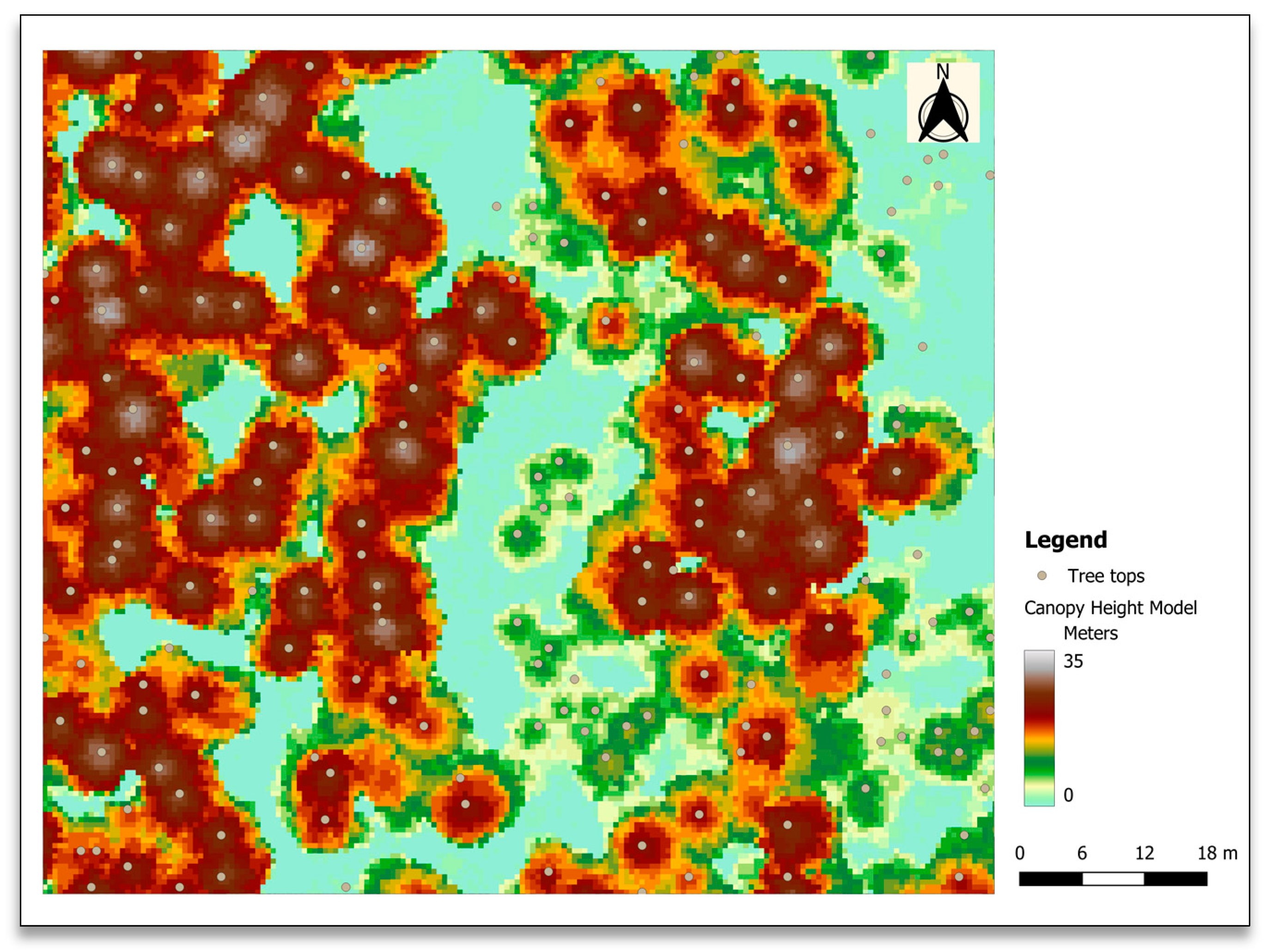
Figure 5.
A subset of the generated tree registry for the Pertouli University Forest (Greece), including the Abies borisii regis tops (points), which indicate their exact geographic position. The canopy height model (CHM), also produced using ALS data, serves as the map background depicting the tree height as a continuous surface.

Figure 6.
The tree density map depicting the number of trees per 2500 sq. m. over the area covered by the Abies borisii regis species, which is the one undergoing harvesting activities on a yearly basis.
Figure 6.
The tree density map depicting the number of trees per 2500 sq. m. over the area covered by the Abies borisii regis species, which is the one undergoing harvesting activities on a yearly basis.

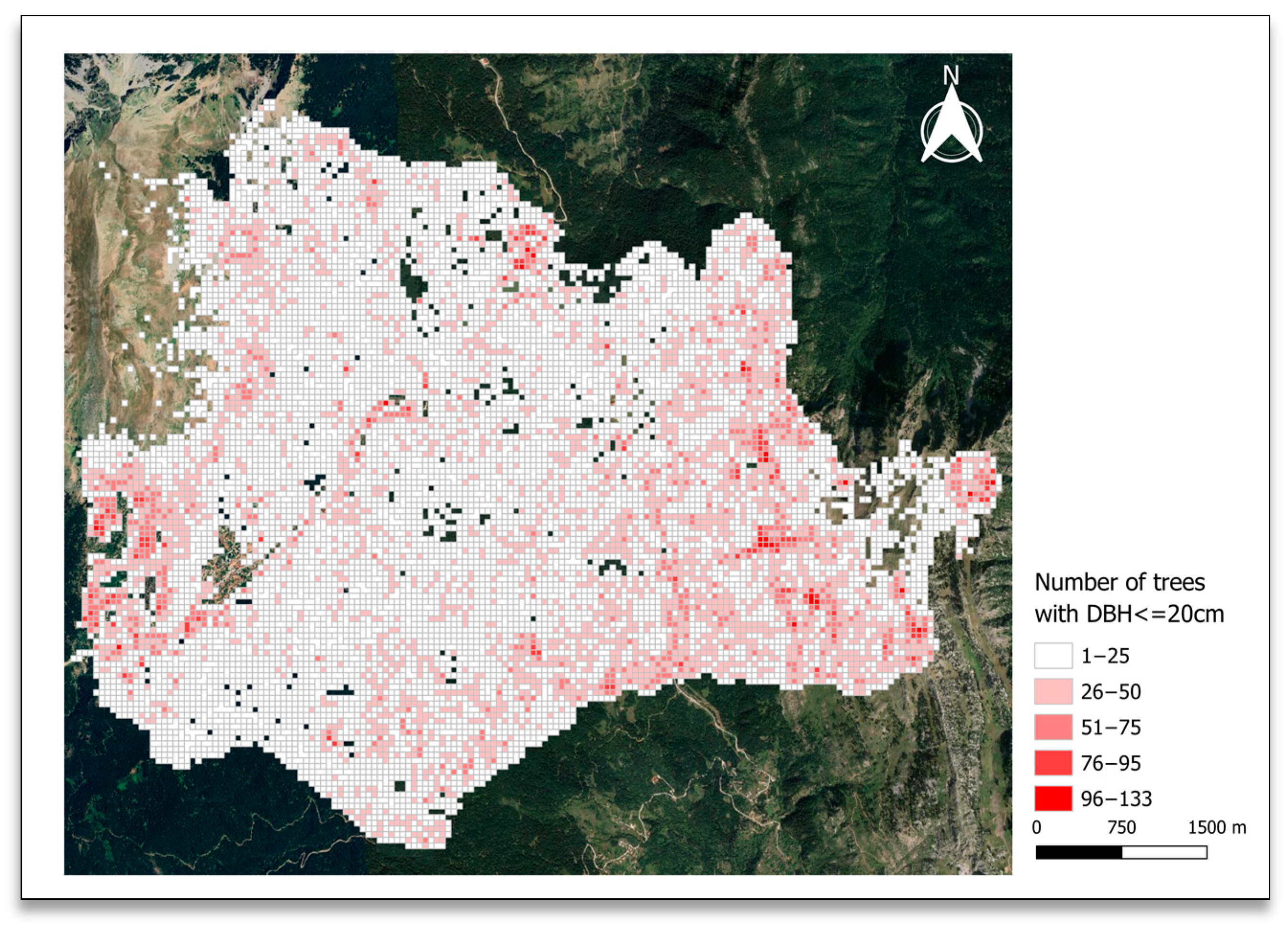
Figure 7.
The tree density map depicting the number of trees with a DBH ≤ 20 cm per 2500 sq. m. over the area covered by the Abies borisii regis species, which is the one undergoing harvesting activities yearly.
Figure 7.
The tree density map depicting the number of trees with a DBH ≤ 20 cm per 2500 sq. m. over the area covered by the Abies borisii regis species, which is the one undergoing harvesting activities yearly.

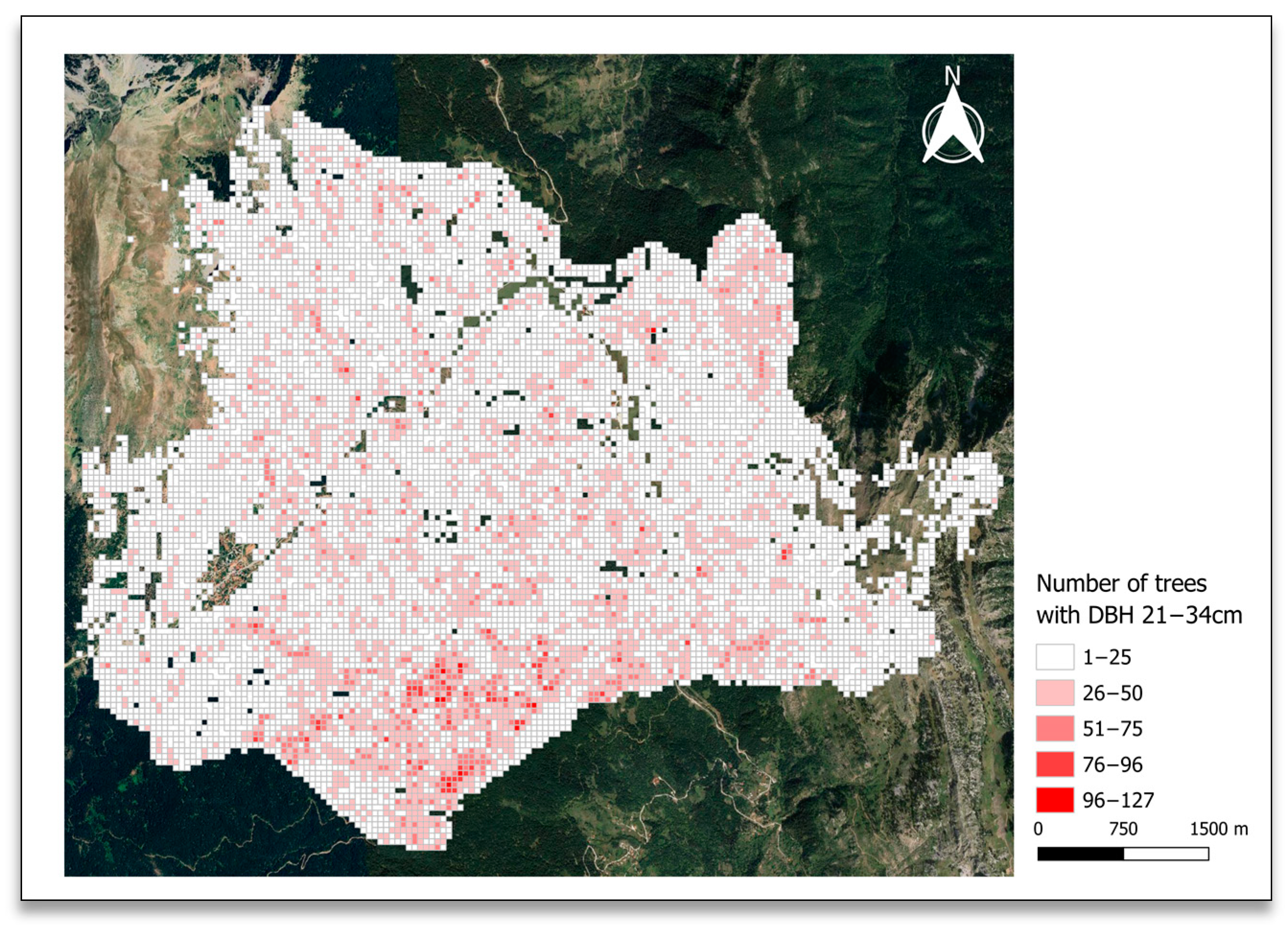
Figure 8.
The tree density map depicting the number of trees with a DBH from 21 to 34 cm per 2500 sq. m. over the area covered by the Abies borisii regis species, which is the one undergoing harvesting activities on a yearly basis.
Figure 8.
The tree density map depicting the number of trees with a DBH from 21 to 34 cm per 2500 sq. m. over the area covered by the Abies borisii regis species, which is the one undergoing harvesting activities on a yearly basis.

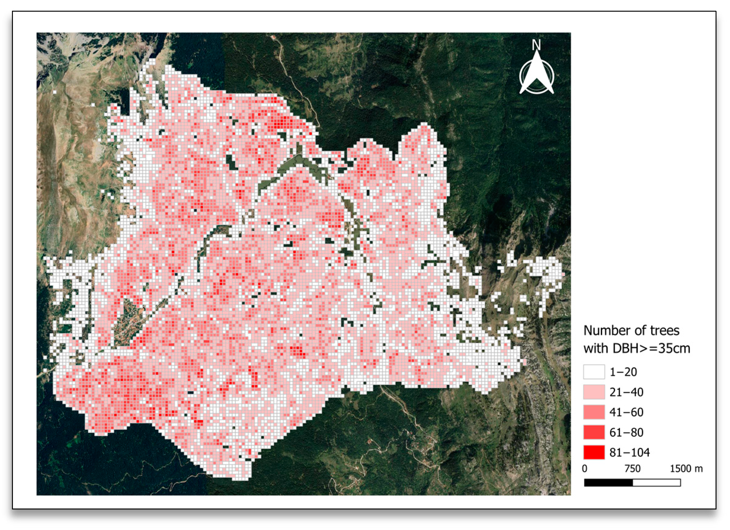
Figure 9.
The tree density map depicting the number of trees with a DBH ≥ 35 cm per 2500 sq. m. over the area covered by the Abies borisii regis species, which is the one undergoing harvesting activities on a yearly basis.
Figure 9.
The tree density map depicting the number of trees with a DBH ≥ 35 cm per 2500 sq. m. over the area covered by the Abies borisii regis species, which is the one undergoing harvesting activities on a yearly basis.

Figure 10.
The reference versus estimated density of the general tree density map produced using the ALS-derived tree registry, which includes trees of DBH (diameter at breast height) classes (i.e., class 1: ≤20 cm, class 2: 21–34 cm, and class 3: ≥35 cm). The red line represents the regression line, while the grey area illustrates the standard error.

Figure 11.
The reference versus estimated density of the tree density map produced using the ALS-derived tree registry, which includes trees of the DBH (diameter at breast height) class 1 (i.e., ≤20 cm). The red line represents the regression line, while the grey area illustrates the standard error.

Figure 12.
The reference versus estimated density of the tree density map produced using the ALS-derived tree registry, which includes trees of the DBH (diameter at breast height) class 2 (i.e., 21–34 cm). The red line represents the regression line, while the grey area illustrates the standard error.

Figure 13.
The reference versus estimated density of the general tree density map produced using the ALS-derived tree registry, which includes trees of the DBH (diameter at breast height) class 3 (i.e., ≥35 cm). The red line represents the regression line, while the grey area illustrates the standard error.

Figure 14.
The reference versus the stem biomass estimated using the tree height and diameter at breast height (DBH) provided by the produced ALS-derived tree registry. The red line represents the regression line, while the grey area illustrates the standard error.
Figure 14.
The reference versus the stem biomass estimated using the tree height and diameter at breast height (DBH) provided by the produced ALS-derived tree registry. The red line represents the regression line, while the grey area illustrates the standard error.

Figure 15.
Graphs illustrating the percentage of detected and undetected trees in each sample plot as a result of the accuracy assessment of the general tree density map, which includes all DBH classes (i.e., all trees) and the three tree density maps, each of which includes trees of an individual DBH class (i.e., DBH class 1, DBH class 2, and DBH class 3, respectively).


Table 1.
Parameters, residual standard error (RSE), R2, adjusted R2, and p-values for the DBH estimation based on the tree height. Parameters a and b are the intercept and the scaling coefficient, respectively.
Table 1.
Parameters, residual standard error (RSE), R2, adjusted R2, and p-values for the DBH estimation based on the tree height. Parameters a and b are the intercept and the scaling coefficient, respectively.
| Equation | Parameters | RSE | R2 | AdjR2 | p-Value |
|---|---|---|---|---|---|
| Tree Height to DBH | a = −4.01594 b = 1.06188 | 0.1956 | 0.8834 | 0.8795 | 1.53 × 10⁻¹⁵ |
Table 2.
The maximum, minimum, and average values of the additional tree parameters were estimated with the use of the generated ALS-derived tree registry (tree height and DBH) and species-specific allometric equations over the entire forest region covered by the Abies borisii-regis species.
Table 2.
The maximum, minimum, and average values of the additional tree parameters were estimated with the use of the generated ALS-derived tree registry (tree height and DBH) and species-specific allometric equations over the entire forest region covered by the Abies borisii-regis species.
| Parameters | Maximum | Minimum | Average |
|---|---|---|---|
| Stem biomass | 4907.16 | 6.27 | 525.41 |
| Dead branches biomass | 13.33 | 0.05 | 2.41 |
| Needles biomass | 1.65 | 0.0009 | 0.17 |
| Branches biomass | 233.63 | 0.19 | 31.91 |
| Bark biomass | 129.54 | 0.37 | 16.51 |
| Total biomass | 5285.33 | 6.89 | 576.44 |
| Sequestrated carbon | 2642.67 | 3.44 | 288.22 |
| Potential total SFL | 378.17 | 0.62 | 51.02 |
| Potential woody SFL | 5283.68 | 6.89 | 576.26 |
| Potential non-woody SFL | 1.65 | 0.0009 | 0.17 |
Table 3.
The goodness-of-fit statistical measures obtained from the comparison of the four produced tree density maps (illustrating the total and per DBH class number of trees at a 50 m × 50 m spatial resolution) and the estimated stem biomass for each tree with the respective parameters of the forest management plan of the year 2018. DBH class 1 includes the trees with a DBH ≤ 20 cm, DBH class 2 refers to trees with a DBH between 21 and 34 cm, and DBH class 3 includes the trees of a DBH ≥ 35 cm.
| Variable | R2 | AdjR2 | RSE |
|---|---|---|---|
| Tree density (total) | 0.14 | 0.12 | 5.72 |
| Tree density (DBH class 1) | 0.15 | 0.12 | 5.09 |
| Tree density (DBH class 2) | 0.20 | 0.18 | 5.21 |
| Tree density (DBH class 3) | 0.61 | 0.60 | 5.15 |
| Stem biomass | 0.67 | 0.66 | 1813 |
Disclaimer/Publisher’s Note: The statements, opinions and data contained in all publications are solely those of the individual author(s) and contributor(s) and not of MDPI and/or the editor(s). MDPI and/or the editor(s) disclaim responsibility for any injury to people or property resulting from any ideas, methods, instructions or products referred to in the content. |
© 2023 by the authors. Licensee MDPI, Basel, Switzerland. This article is an open access article distributed under the terms and conditions of the Creative Commons Attribution (CC BY) license (https://creativecommons.org/licenses/by/4.0/).
Share and Cite
MDPI and ACS Style
Georgopoulos, N.; Stefanidou, A.; Gitas, I.Z. Supporting Operational Tree Marking Activities through Airborne LiDAR Data in the Frame of Sustainable Forest Management. Forests 2023, 14, 2311. https://doi.org/10.3390/f14122311
AMA Style
Georgopoulos N, Stefanidou A, Gitas IZ. Supporting Operational Tree Marking Activities through Airborne LiDAR Data in the Frame of Sustainable Forest Management. Forests. 2023; 14(12):2311. https://doi.org/10.3390/f14122311
Chicago/Turabian StyleGeorgopoulos, Nikos, Alexandra Stefanidou, and Ioannis Z. Gitas. 2023. "Supporting Operational Tree Marking Activities through Airborne LiDAR Data in the Frame of Sustainable Forest Management" Forests 14, no. 12: 2311. https://doi.org/10.3390/f14122311
Note that from the first issue of 2016, this journal uses article numbers instead of page numbers. See further details here.