
Improving the Gross Primary Production Estimate by Merging and Downscaling Based on Deep Learning


1
Key Laboratory of Ecosystem Carbon Source and Sink, School of Atmospheric Science & Remote Sensing, Wuxi University, Wuxi 214105, China
2
National Climate Center, China Meteorological Administration, Beijing 100081, China
3
Shandong Climate Center, Jinan 250031, China
*
Author to whom correspondence should be addressed.
Forests 2023, 14(6), 1201; https://doi.org/10.3390/f14061201
Submission received: 24 April 2023
/
Revised: 25 May 2023
/
Accepted: 8 June 2023
/
Published: 9 June 2023
(This article belongs to the Special Issue Applications of Artificial Intelligence in Forestry)
Abstract
:A reliable estimate of the gross primary productivity (GPP) is crucial for understanding the global carbon balance and accurately assessing the ability of terrestrial ecosystems to support the sustainable development of human society. However, there are inconsistencies in variations and trends in current GPP products. To improve the estimation accuracy of GPP, a deep learning method has been adopted to merge 23 CMIP6 data to generate a monthly GPP merged product with high precision and a spatial resolution of 0.25°, covering a time range of 1850–2100 under four climate scenarios. Multi-model ensemble mean and the merged GPP (CMIP6DL GPP) have been compared, taking GLASS GPP as the benchmark. Compared with the multi-model ensemble mean, the coefficient of determination between CMIP6DL GPP and GLASS GPP was increased from 0.66 to 0.86, with the RMSD being reduced from 1.77 gCm−2d−1 to 0.77 gCm−2d−1, which significantly reduced the random error. Merged GPP can better capture long-term trends, especially in regions with dense vegetation along the southeast coast. Under the climate change scenarios, the regional average annual GPP shows an upward trend over China, and the variation trend intensifies with the increase in radiation forcing levels. The results contribute to a scientific understanding of the potential impact of climate change on GPP in China.
1. Introduction
Global climate change, especially the impact of climate warming on the human living environment, has attracted more and more attention [1]. With the continuous development of the global industry, the use of fossil fuels is increasing. This process releases large amounts of carbon dioxide and changes the proportions of greenhouse gases, causing global climate problems such as the intensification of the greenhouse effect. The gross primary productivity (GPP), formed by terrestrial vegetation through photosynthesis to fix CO2 and energy in the biosphere, is the initial stage of entering the carbon cycle process and the basis of the ecosystem carbon cycle [2]. Terrestrial ecosystems can influence global climate change through the carbon cycle [3]. Therefore, the research on the carbon cycle of global terrestrial ecosystems has received widespread attention and has become a hot spot in global change research [4].
An essential indicator of terrestrial ecosystem carbon cycle research is GPP. The gross primary productivity, that is, the total photosynthetic uptake or carbon assimilation by plants, is a key component of terrestrial carbon balance [5]. It is the main driving factor of the terrestrial carbon sink, which is responsible for absorbing about 30% of anthropogenic carbon dioxide emissions [6]. In general, it can be said that GPP plays a vital role in the global carbon cycle [7,8,9,10]. Characterizing the spatiotemporal changes and trends of GPP is essential for a deeper understanding of the carbon cycle between terrestrial ecosystems and the atmosphere [11]. Therefore, quantifying the GPP is crucial to understand the impact of climate change and atmospheric carbon dioxide concentration changes on the terrestrial carbon cycle [12,13]. The accurate estimation of GPP at regional and even global scales contributes to a more comprehensive and in-depth understanding of ecosystem functions and the global carbon cycle [14]. However, with the intensification of climate change, there is significant uncertainty in estimating GPP [15].
In recent decades, significant progress has been made in estimating GPP, and many global GPP datasets have been published [16]. These products differ in GPP estimates in different ecosystems and external environments, with advantages and disadvantages in various studies [17,18,19]. Data-driven GPP estimation is the primary tool for GPP research and model evaluation. It mainly includes the following three types. The first type uses eddy covariance (EC) technology to obtain flux tower observation and upscaling [20]. Process-based models such as the Community Land Model (CLM) are commonly considered in the revision of GPP products [21]. However, the distribution of flux towers is sparse and uneven, and the coverage period is different and limited [22], which makes the derivation of global GPP complicated. When estimating GPP products by scaling up, there will be a more significant deviation near the sparse flux tower [22]. The second type is the machine learning (ML) method that uses satellites and other meteorological data as input [23,24,25,26,27,28]. ML products are widely used for benchmarking and depend more on the spatial representation of flux sites [15,24]. The third type is based on the principle of light use efficiency (LUE), which is used to derive the GPP based on optical remote sensing variables [22,27,29,30,31]. LUE products are good at detecting the spatial distribution pattern of GPP; however, they usually perform poorly in seasonal estimation and overestimate GPP under dry and cold conditions [28,32,33,34,35]. At the regional and even global scale, the land surface model (LSM) and ecosystem model [36,37,38] are also effective methods to simulate GPP. The process models consider plant physiological and ecological processes, which have solid theoretical significance and can simulate future productivity changes. LSM products are more consistent in spatiotemporal distribution and better in response to climate change, but various model parameters, input data, and model structures cause more significant uncertainty [15,39,40]. Especially in large-scale applications, the accuracy of the model is affected to some extent [41].
However, the current GPP products rely on assumptions. They are based on different estimation models so that no GPP product group can perform consistently better in diverse ecosystems and external conditions [42]. In particular, there is significant uncertainty in CMIP6 datasets under future climate change scenarios. The uncertainties in climate prediction are relevant to the modelling of GPP, although they are independent of the estimation method of GPP. As a result, the changes and trends obtained from different GPP products are often various [43], leading to unconvincing research results of a single GPP product [44]. Therefore, to overcome the limitations of a single dataset of GPP products, the question of how to effectively merge multiple datasets has been raised. Studies have shown that the multi-model ensemble mean is better than the single model in estimating GPP [17,45]. Traditionally, the IPCC report shows that the average value of multiple models is the best. Empirical evidence from various modelling fields indicates that the multi-model ensemble mean eliminates at least some deviations from the single model, which can produce better predictions or values closer to observation [46,47,48,49]. However, the simple multi-model ensemble mean depends on the assumption that the uncertainty of each dataset is the same [50]. However, this assumption is not reasonable from the differences between datasets.
On the other hand, the spatial resolutions between prediction CMIP6 GPP datasets are generally low and mismatched. At present, bilinear interpolation is widely used for downscaling. Super-Resolution Convolution Neural Network [51] is a pioneering work of image super-resolution reconstruction. It makes people pay attention to the deep learning convolution neural network, the performance of which is superior to the traditional super-resolution. A neural network called Ynet [52] combines image super-resolution and data merging technology, which has been further used for soil moisture data merging with excellent results [53]. It establishes the relationship between reference data and multi-model datasets in the historical period to generate a merged GPP product with the distribution characteristics of reference data. Furthermore, GPP-merged data in the projection period under multiple climate scenarios can be obtained based on 23 CMIP6 model projections if the relationship built during the historical period is applied to the projection period. The evaluation in the historical period shows that the quality of the merged data is significantly improved compared with the multi-model ensemble mean, indicating that the merged data are reliable. Therefore, the variation trends in GPP under multiple climate scenarios in the future were further analyzed based on the merged data.
This study aims to produce an improved high-resolution merged GPP dataset by adopting a new method to combine the advantages of 23 CMIP6 GPP datasets, without relying on any prior knowledge, to analyze the long-term variation trends in GPP under multiple climate scenarios in the future based on the improved merged data. Based on the historical CMIP6 GPP data, the deep learning method called Ynet [52] neural network is used to train the deep learning model with merging and downscaling functions. The 23 groups of monthly GPP datasets are integrated into this high-resolution long-series dataset called CMIP6DL GPP. The period and the spatial resolution are 1850–2100 and 0.25 degrees. The future projection period includes four climate change scenarios, such as SSP1-2.6, SSP2-4.5, SSP3-7.0, and SSP5-8.5. The performance of the merged product has been evaluated based on eddy covariance tower GPP data, and the effectiveness of the merging method has been discussed. Finally, the variation trends of GPP over China under future climate change scenarios have been analyzed based on CMIP6DL GPP.
2. Materials and Methods
2.1. Study Area
This study takes China as the research region. The climate characteristics of China are complex and various, with a monsoon climate in the east, a temperate continental climate in the northwest, and an alpine climate in the Qinghai–Tibet Plateau. In general, the climate in China is characterized by a monsoon climate with a high temperature, a rainy summer and cold winter with little rain. The high-temperature period is consistent with the rainy period in the study region. There is apparent spatial heterogeneity in GPP due to the differences in topography, vegetation types, and hydrothermal conditions in the different areas [54]. The growth of vegetation is closely related to the climate of the region where it is located. Therefore, according to the Coben climate division and the classic climate division of China, China is divided into four climatic parts for regional analysis: the arid, semi-arid, semi-humid, humid, and Qinghai–Tibet Plateau regions.
2.2. GLASS GPP Data
Global Land Surface Satellite (GLASS) gross primary production (GPP) is a global surface remote sensing product with a long time series and high precision based on multi-source remote sensing data and ground observation [45]. The Bayesian multi-algorithm integration method integrates eight widely used light use efficiency (LUE) models, including CASA, CFix, CFlux, EC-LUE, MODIS, VPM, VPRM, and two-leaf. The spatial and temporal resolution of GLASS GPP are 5 km and eight days, from 1982 to 2018. The unit of the data is gCm−2d−1. The development and validation of the algorithm are based on the data from global fluxnet, which contains nine types of terrestrial ecosystems, such as evergreen broad-leaved forest, evergreen coniferous forest, deciduous broad-leaved forest, mixed forest, temperate grassland, tropical savanna, shrub, farmland, and tundra. GLASS GPP can be downloaded from http://www.geodata.cn (accessed on 23 April 2023).
2.3. CMIP6 GPP Data
The monthly GPP data from 23 available CMIP6 models are used in the study, with the unit of kgCm−2s−1. The period is over 1850–2100, including the historical and future projection period. More specifically, the projection period of 2015–2100 contains the four most interesting scenarios: SSP1-2.6, SSP2-4.5, SSP3-7.0, and SSP5-8.5. The model and GLASS GPP data are first uniformly interpolated to 2° due to the inconsistent spatial resolution. Meanwhile, it is necessary to unify the unit of model simulation data and GLASS GPP to gCm−2d−1. The first member, r1i1p1f1, is selected if possible (r1i1p1f2 is used if unavailable). CMIP6 GPP can be downloaded from https://esgf-node.llnl.gov/projects/cmip6/ (accessed on 9 June 2023). The information on the 23 models used is listed in the Table 1 below.
2.4. Deep Learning Network
In this study, a GPP-merged product conforming to the distribution characteristics of the GLASS GPP dataset is developed by merging the simulated data of CMIP6 models. A neural network named Ynet [51] is adopted in the data merging part, which combines data merging and image super-resolution technology. The deep learning model establishes relationships between the reference and the CMIP6 GPP data in the historical period and is then applied in future projections. Compared with the multi-model ensemble mean, the merged data have higher accuracy and spatial resolution over 1850–2100 in China. The multi-model ensemble mean is a simple average of the simulation results of the 23 CMIP6 models. It uses the simplest strategy of assuming that all 23 model data have the same uncertainty; thus, the multi-model ensemble mean is a simple average of each model. The merged data in this study are generated based on the deep learning method, which compensates for this deficiency. The novelty of the deep learning method used in this study is that it combines data merging and image super-resolution technology, which combines the advantages of 23 CMIP6 GPP datasets without relying on any prior knowledge.
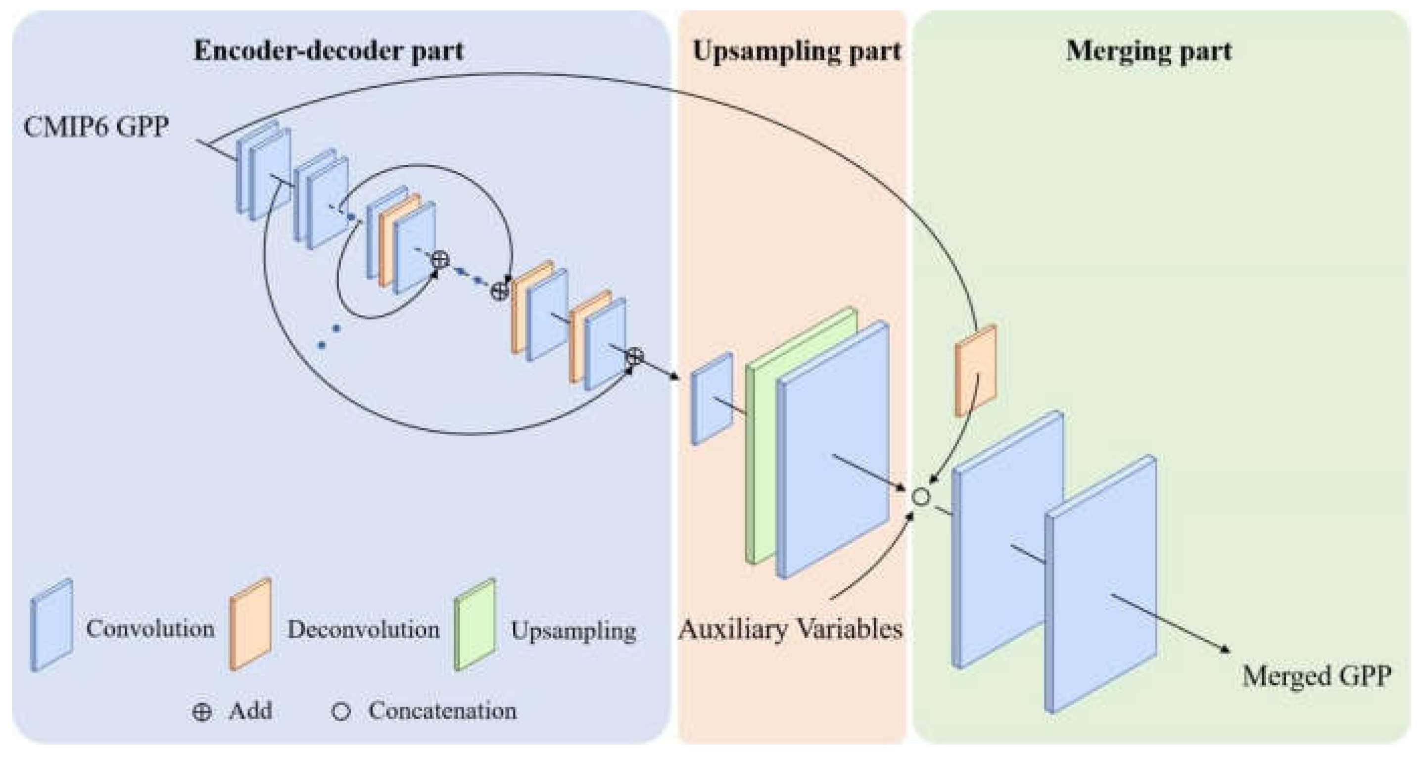
The model architecture is shown in Figure 1. This structure consists of three parts. The first part is a symmetric encoder-decoder structure with a skip connection. Similar to the residual encoder-decoder network, this structure solves the problem of gradient disappearance when the error calculated by the loss function in the model training process is propagated back. This structure captures the abstract features of low-resolution images with noise and outputs a “cleaner” image, which can be regarded as a feature extractor. In addition to the 30 convolutional layers, this part also contains 15 deconvolution layers. It may introduce “checkerboard artefacts”, resulting in lower image output quality [55]. Therefore, to reduce the problem, a convolutional layer is added after each deconvolution layer to compensate for upsampling. Specifically, this part’s input to the model is low-resolution CMIP6 GPP. The second part of the model is upsampling, which is mainly used for downscaling. It consists of one upper sampling layer using bilinear interpolation and two convolution layers with the same feature depth as the input channel. As in the first part, the last two convolution layers were added to eliminate the checkerboard effect.
The third part is data merging, which consists of three input datasets, including upsampling output, auxiliary data, and unsampled CMIP6 GPP. The three datasets calculated by the two convolution layers are joined to obtain high-resolution data. Among them, auxiliary data are used to help improve the results, which remained constant throughout different months over the training and testing periods. The loss function can be calculated according to the following formula:
Among them, θ is the network parameter that needs to be optimized. f(Xi, θ) represents the learned function. In addition, n is the total number of training samples. X and Y represent the input data and the target at position i.
2.5. Evaluation Indicators
The evaluation indicators, including mean absolute error (MAE), root mean square deviation (RMSD), unbiased root mean square deviation (ubRMSD), and coefficient of determination (r2), have been used to assess the performance of the merged data objectively and find out if it captures the distribution characteristics of the reference data. The calculation formulae are as follows:
where n represents the total number of samples. Mi and Ri represent the merged and reference data at i, respectively. and represent the average of the merged and reference data.
2.6. Deep Learning Merging Model Training
Statistical analysis (Figure S1) shows that GPP data belong to heavy-tail distribution. The characteristic of the skewed distribution data is that there are more samples with little influence and fewer samples with substantial impact. The concrete manifestation in GPP data is that the number of pixels near the value of 0 is far more than that of other values. In addition, the larger the value, the smaller the number of pixels. Such datasets will make the deep learning network perform well in the low-value range, while the efficiency is relatively low in the high-value range, resulting in overall reduced accuracy. Therefore, the log1p function converts GPP data to make it more obedient to Gaussian distribution during data preprocessing.
The period from 1982 to 2014, when CMIP6 GPP data and GLASS GPP data coincide, was selected to establish the relationship between input data and reference data using the deep learning network. The GPP data simulated by 23 CMIP6 models and the reference data in the same month were matched as a group, totaling 396 samples. All samples were divided into three datasets according to time: training (1982–2010), validation (2011–2012), and test dataset (2013–2014). The number of iterations and the initial learning rate were 150 times and 1 × 10⁻⁴ during the training stage, respectively.
Figure 2 shows loss function curves for training and validation datasets. As shown in the figure, the loss reduced sharply in the first ten iterations of the training process. Subsequently, it shows a fluctuant reduction. The model is stable after 77 iterations, with a decreased loss. Loss no longer changes after 112 iterations, indicating that the model has been trained.
3. Results
3.1. Quality Evaluation of Merging Results
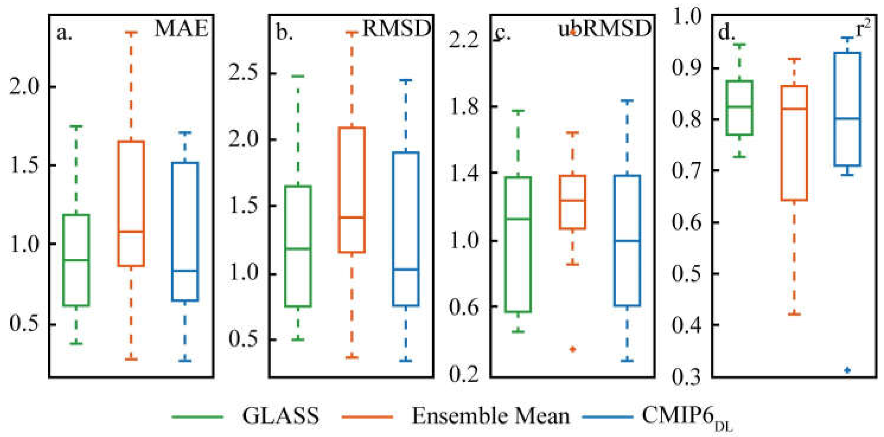
The trained merging model has been tested. The results of comparing GLASS GPP, CMIP6DL GPP, and multi-model ensemble mean with fluxnet data in China are shown in Figure 3. However, the results only represent the accuracy of the ten sites, as there are only ten unevenly distributed flux towers in China. As can be seen from the figure, all three datasets have a wide distribution range in the four indicators. The distribution range in MAE, RMSD and r2 of the multi-model ensemble mean is wider than that of the other two datasets, indicating that it has a higher uncertainty. Although the distribution range is relatively small on ubRMSD, many outliers exist in the multi-model ensemble mean. The uncertainty of CMIP6DL GPP is lower compared with the multi-model ensemble mean, while the median performs the best in MAE, RMSD, and ubRMSD. The merged data have improved overall (Figure 3a–c), indicating that data are closer to the actual value than the multi-model ensemble mean.
Table 2 shows the model’s performance on the test dataset taking GLASS GPP as the benchmark, with the results showing that the merged GPP has improved in the aspect of the four indices and has a higher accuracy in China as a whole compared with the multi-model ensemble mean.
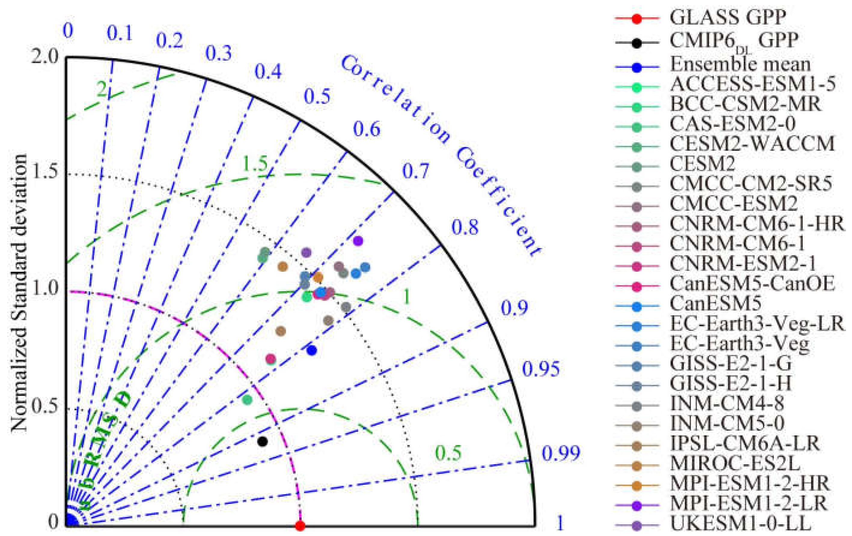
The normalized Taylor diagram obtained by calculating correlation coefficients, ubRMSD, and standard deviation ratios is used to evaluate further the CMIP6DL GPP, CMIP6 GPP, and muti-model ensemble mean. GLASS GPP has been used as the reference due to its relatively low uncertainties. Figure 4 shows the distribution of correlation coefficient, ubRMSD, and standard deviation ratio between 25 datasets (including CMIP6DL GPP, the multi-model ensemble mean, and 23 CMIP6 datasets) and the reference data in 2013–2014. As shown in Figure 4, the red dot represents GLASS GPP. Since it is used as reference data, the correlation coefficient and standard deviation ratio are equal to 1, and ubRMSD is 0. The black dot represents CMIP6DL GPP data, which is the closest to the red dot in the figure, indicating that the overall performance of CMIP6DL GPP data is better than that of all datasets simulated by other models. The correlation coefficient of all CMIP6 GPP is less than 0.82, and ubRMSD is greater than 0.5. There are significant differences among the 23 model data, of which CAS-ESM2-0 performs the best, even better than the multi-model ensemble mean. The multi-model ensemble mean is still superior to most single CMIP6 data, though it is affected by the high error of model data. In general, CMIP6DL GPP data perform the best in all aspects.
To evaluate the spatial accuracy of the merged data, the spatial absolute error distributions of CMIP6DL GPP, the multi-model ensemble mean, and GLASS GPP are plotted, respectively. Figure 5a shows the MAE between CMIP6DL GPP and GLASS GPP in the test dataset, with the results showing that the regions with MAE less than 0.5 account for 73.91%. The errors in Northwest, Northeast, and North China are generally minor, less than 0.21 gCm−2d−1. However, the effects of CMIP6DL GPP in Central China and the eastern part of Southwest China are not ideal, with the error ranging from 0.5 to 1.5 gCm−2d−1, with a total of 7.4% of the regional errors being even more significant than 1 gCm−2d−1. Relatively large errors mainly occur in Yunnan Province, with two-thirds of the regional errors being more significant than 0.5 gCm−2d−1. Figure 5b shows MAE between the multi-model ensemble mean and GLASS GPP. Except for Northwest China, the error in most regions is beyond 1 gCm−2d−1. Specifically, the regions with an error greater than 1 gCm−2d−1 account for 45.17%, even more significant than 2 gCm−2d−1 in Central, East, and South China. In summary, CMIP6DL GPP generated by merging the model Ynet is highly reliable.
3.2. Assessment of the Variations in the Merged GPP
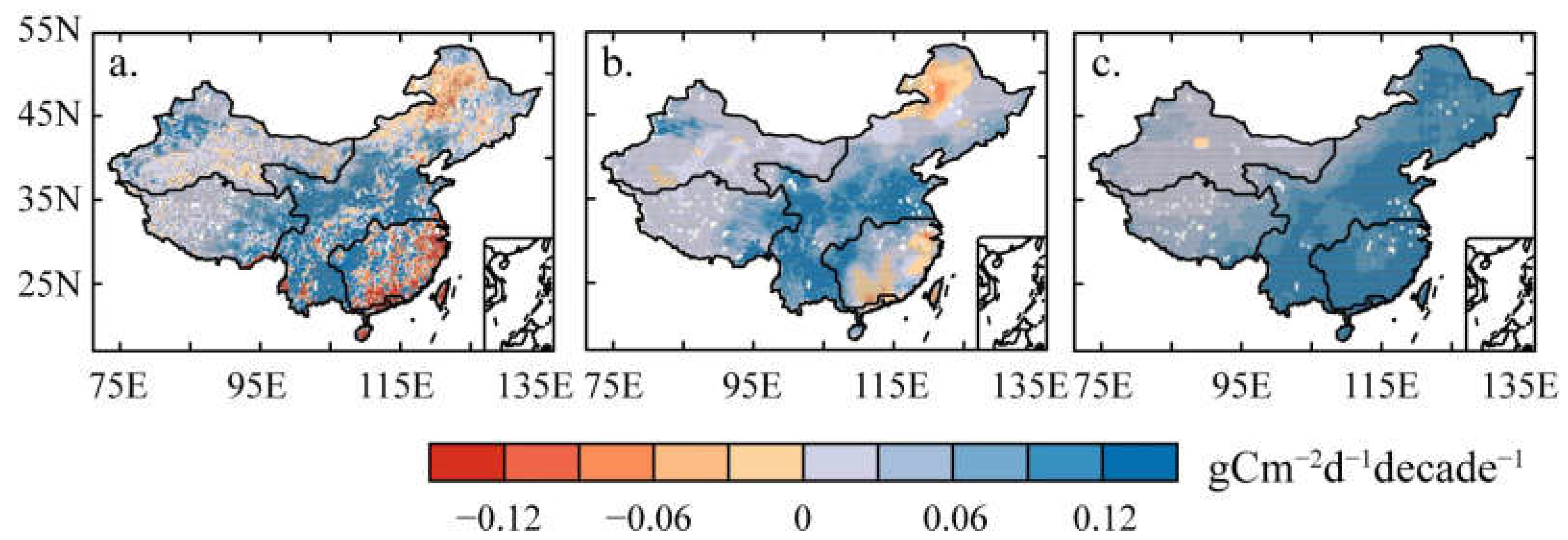
GLASS GPP is a dataset generated by the light use efficiency model integrating CO2, radiation, and vapor pressure deficit (VPD), providing a reliable long-term GPP estimation. Figure 6 shows the long-term changes in GLASS GPP, CMIP6DL GPP, and multi-model ensemble mean from 1982 to 2014. As shown in Figure 6a, the variations in GLASS GPP are not apparent and almost remain unchanged in the northwest arid regions. There is an increasing trend in Central China and a significant decrease in the eastern part of Inner Mongolia, the southern part of East China, and South China. The long-term changes in the multi-model ensemble mean are shown in Figure 6c. There is a sharp increasing trend throughout China, except for the western regions. The characteristics of the decrease in the southern coastal areas and Inner Mongolia are not captured, which is inconsistent with the spatial characteristics of the variations in GPP over China. Figure 6b describes the spatial distribution of the long-term variations of the merged GPP data, similar to GLASS GPP. However, the variations are gentler than the reference data since the deep learning merging model is built using a convolution neural network with a “smoothing” effect. That is, it is impossible for the deep learning merging model to learn the extreme value. Compared with the multi-model ensemble mean, the data quality has been significantly improved in eastern Inner Mongolia and South China, dramatically increasing the merged dataset’s reliability in the projection period.
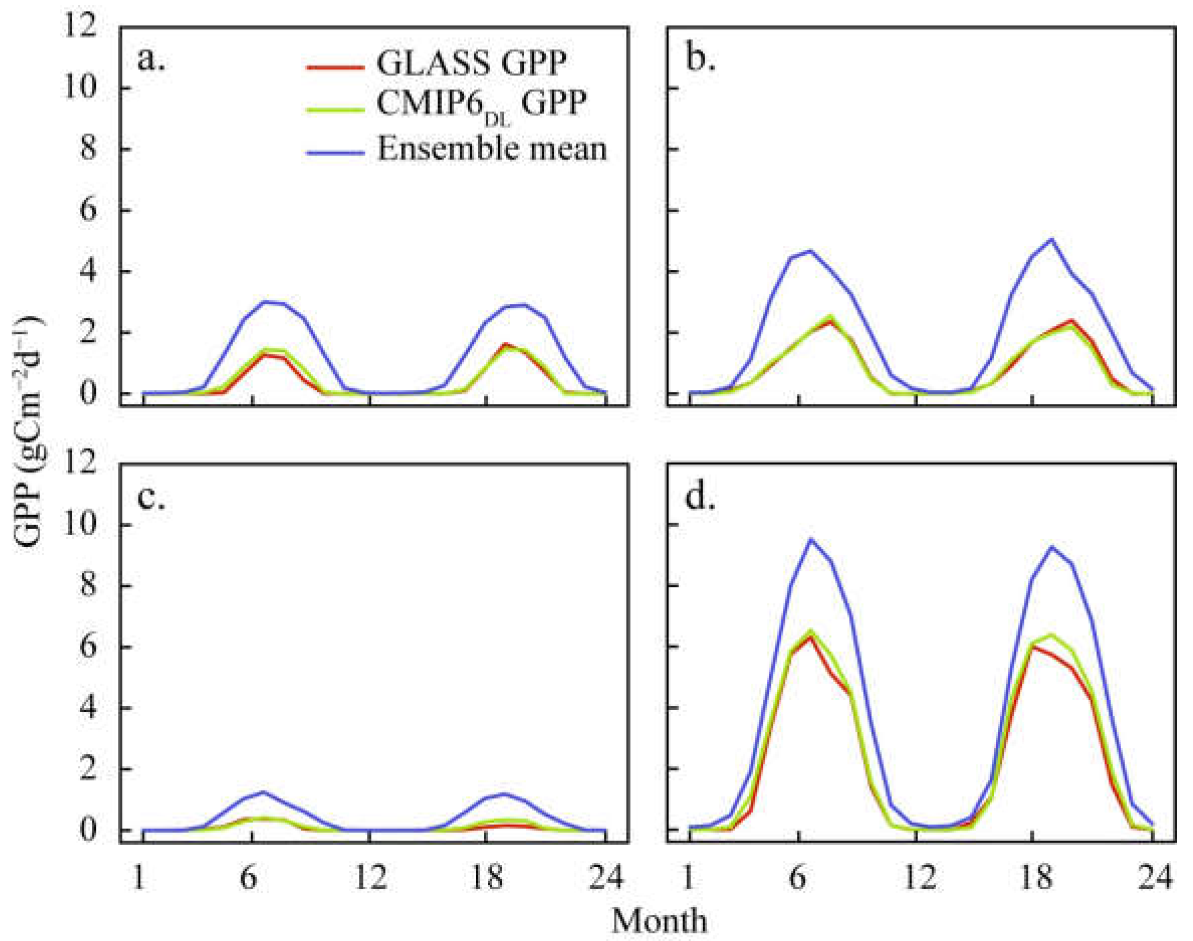
To evaluate the differences in the merged results in the time dimension, the grids are randomly selected in four climatic regions over China (arid, semi-arid and semi-humid, humid region, and Qinghai–Tibet Plateau) to test the time series. As can be seen from Figure 7, there are similar seasonal fluctuations in the three datasets. The fluctuation range of the test dataset is highly consistent in the CMIP6DL GPP and the reference data, while it is more significant in the multi-model ensemble mean. GPP has consistently been overestimated throughout the period in the multi-model ensemble mean. As the GPP increases, the error of the multi-model ensemble mean increases. Specifically, the high value of GPP is concentrated in June and July, when the error of the multi-model ensemble mean is the largest. The impacts of temperature, water, solar radiation, and vegetation growth are the main causes of seasonal variation. The temperature, precipitation, vegetation leaf area, and solar radiation of each region reach the highest values during in the year in summer, and then gradually decrease. The comprehensive impact of these factors ultimately leads to an inverted U-shaped change in the average monthly GPP of each vegetation coverage area.
3.3. Temporal and Spatial Distribution of Merged GPP in Historical Period
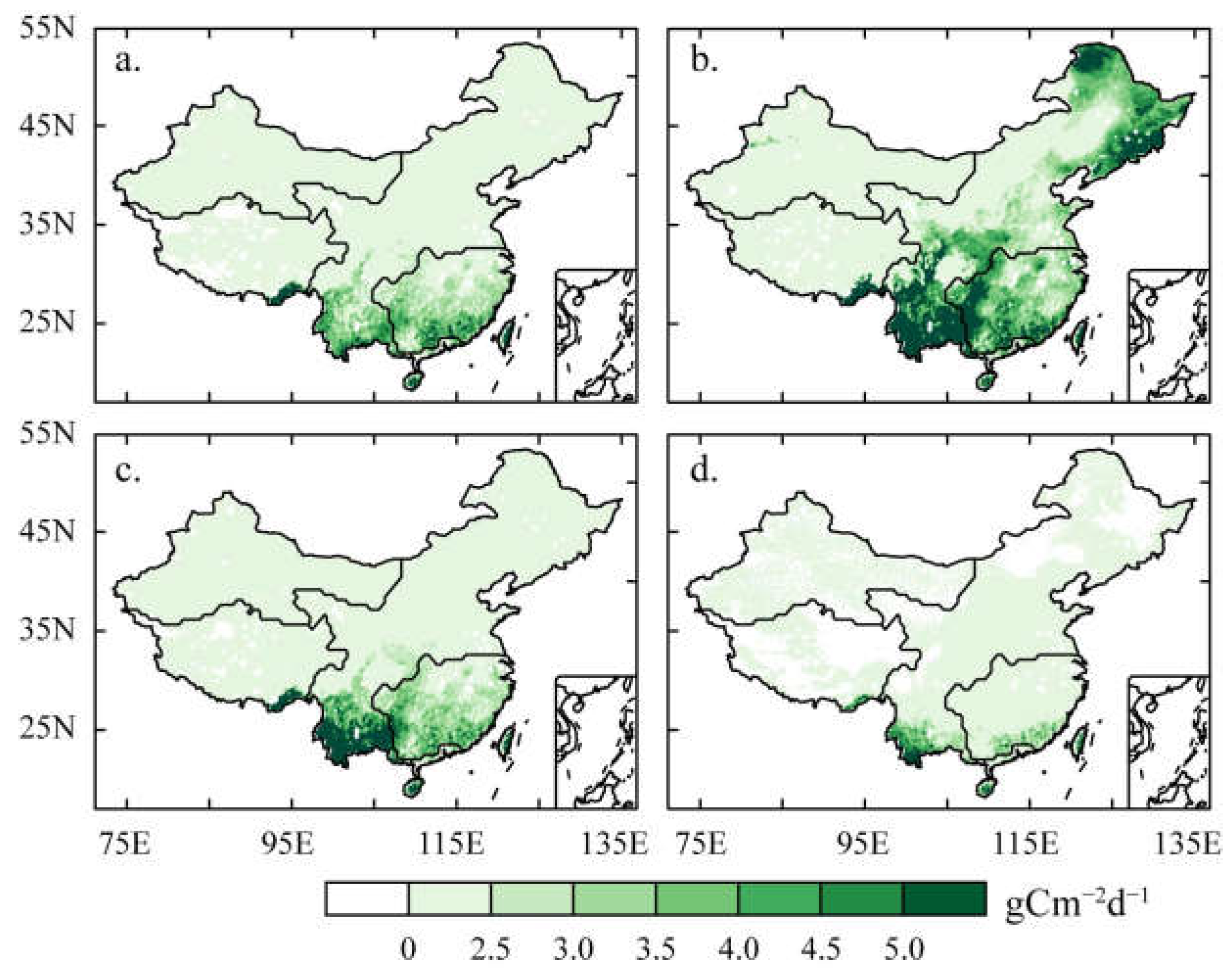
The GPP data over the historical period (1850–2014) and the four climate scenarios (SSP1-2.6, SSP2-4.5, SSP3-7.0, SSP5-8.5) are merged using the trained deep learning merging model based on the data simulated by 23 CMIP6 models. The spatial distribution of GPP in different seasons is shown in Figure 8 to study the seasonal variation characteristics during the historical period (1850–2014). There is a significant spatial distribution gradient of GPP in various seasons in China, mainly due to land use and cover conditions and temperature and water environmental factors. In southern China, the climate is warm and humid, with the best hydrothermal conditions, sufficient sunlight and high light utilization efficiency, high vegetation coverage, and the highest GPP in the growing season. GPP is high in northeast forest regions in summer. However, photosynthesis is inhibited by low temperature in other seasons, resulting in relatively low GPP. In the deserts of the northwest, most areas of the Qinghai–Tibet Plateau, and the grasslands in central and western Inner Mongolia, the plant growing season is relatively short due to water stress and low-temperature constraints, which leads to low productivity and even the lowest GPP. Overall, GPP decreases from southeast to northwest and coastal to inland, consistent with current research results [56,57,58,59]. The spatial distribution of GPP is highly compatible with precipitation in summer, indicating that precipitation is an important factor affecting the distribution of GPP in China. In addition, the GPP near the Tianshan Mountains in Xinjiang is relatively high in summer. The prevailing westerly winds from the Atlantic Ocean and the airflow from the Arctic Ocean encounter the uplift of mountain slopes and generate intense precipitation, which promotes a high vegetation coverage in the west and northwest of the Tianshan Mountains [60]. At the same time, the high mountain snowmelt in the Tianshan Mountains also plays a promoting role.
The spatial distribution of GPP during the four seasons is significantly different, mainly due to the comprehensive influences of the monsoon climate and vegetation type. Throughout the whole year, GPP is the highest in summer (June to August), followed by spring (March to May), autumn (September to November), and the lowest in winter, which entirely fits within the ecological definition of the GPP itself. In spring, the high value of GPP is concentrated in the area south of 28° N. As the summer monsoon moves northward, the temperature in most parts increases, with the average GPP in the historical period reaching 13.6 gCm−2d−1. The spatial distribution of GPP is highly affected by hydrothermal conditions. Thus, the high value is mainly distributed in Yunnan and Guizhou. In autumn, the spatial distribution is similar to that in spring due to the decrease in temperature in northern China. GPP is mostly lower than 1 gCm−2d−1 in winter, and even 0 in some regions. Due to the minimum precipitation and temperature in winter, most of the vegetation is in the non-growing season, which makes the vegetation coverage the lowest, resulting in the lowest GPP throughout the year. Although crops are sown in the north, they grow slowly due to the low temperature. On the contrary, the GPP in southern Yunnan remains high even in winter (Figure 8d).
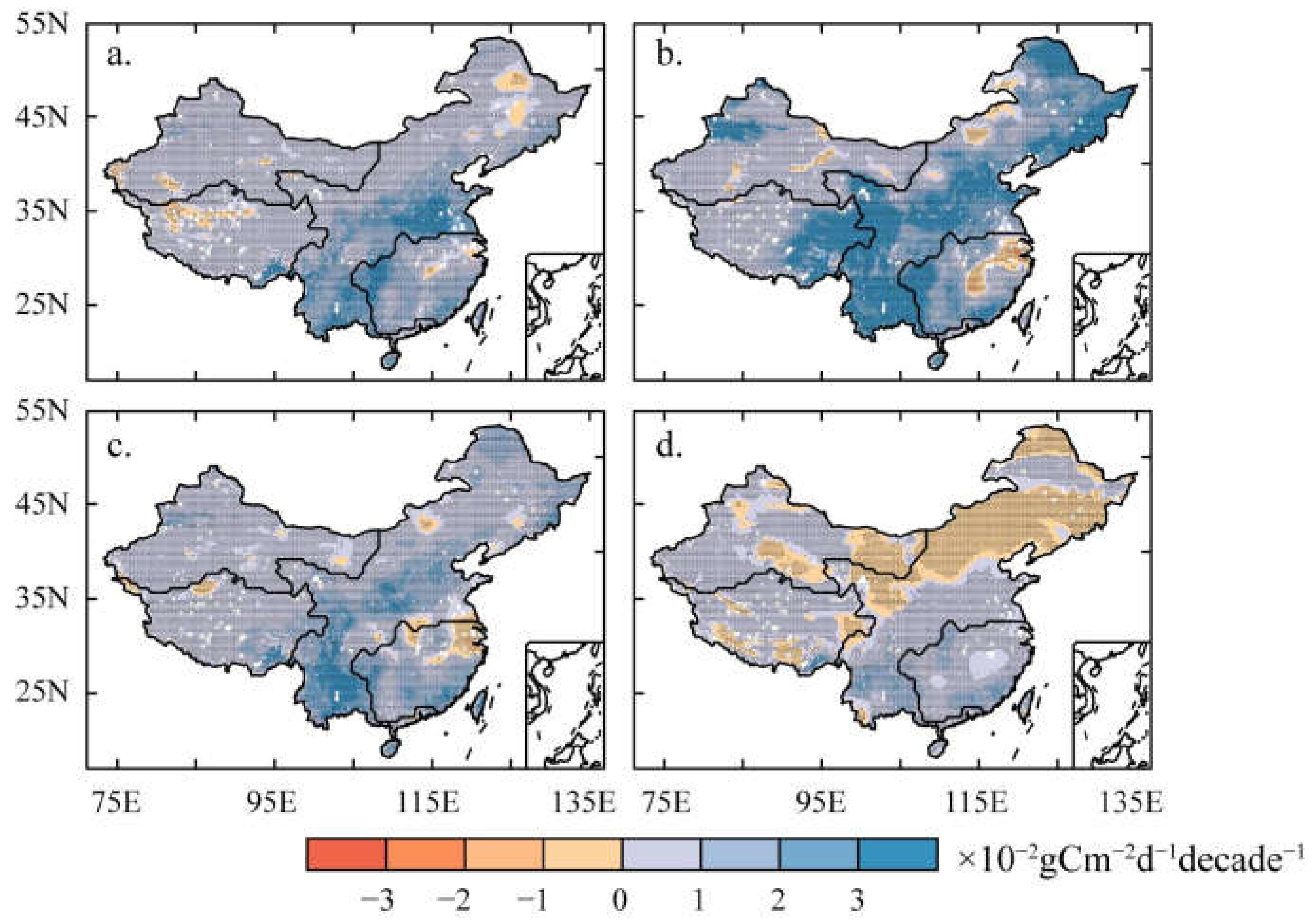
The global climate has undergone significant changes in the past few decades, including frequent extreme climate disasters and sustained warming. Ecosystems and terrestrial carbon sinks will be significantly affected by climate change. On the other hand, GPP is greatly influenced by human activity [61]. Although large-scale afforestation benefits vegetation restoration and increases GPP, population growth and rapid economic development have exacerbated urbanization and disrupted the balance of terrestrial ecosystems. These human interventions significantly impact the formation of GPP dynamics [62,63]. Figure 9 shows the spatial distribution of variation trends in GPP in all seasons over China during the historical period (1850–2014). There are increasing trends in most regions; however, changes in these trends exhibit significant heterogeneity in space and time. The trend is the strongest in summer, followed by spring and autumn, and the most gentle in winter. In summer, the variation trend of GPP in more than one-third of the regions is relatively large, concentrated in Northeast China, the south of North China, and the southwest regions. The annual mean value of GPP in these regions is significant, with the variation trends also being substantial. It is mainly related to the superior local water and heat conditions and the suitable climate environment, which results in the overall growth of vegetation. The GPP in the south of Central China and East China shows a weak decreasing trend. It is mainly due to the increase in temperature in the southern region since the 1990s, which increases the frequency of heat waves and drought events [64,65]. There is a negative impact on the terrestrial carbon cycle, resulting in a decline in GPP. Compared with summer, the regions with a substantial increase in autumn tend to reduce; meanwhile, the trend is gentler. In spring, the increasing trends concentrate in Anhui and Guizhou. In winter, there is a trend of widespread decline in Inner Mongolia, Jilin, and Liaoning, accounting for 31.57% of the whole region, while there is an increasing trend in some regions in the south.
3.4. Long-Term Changes in Merged GPP in Projection Period under Multiple Climate Scenarios
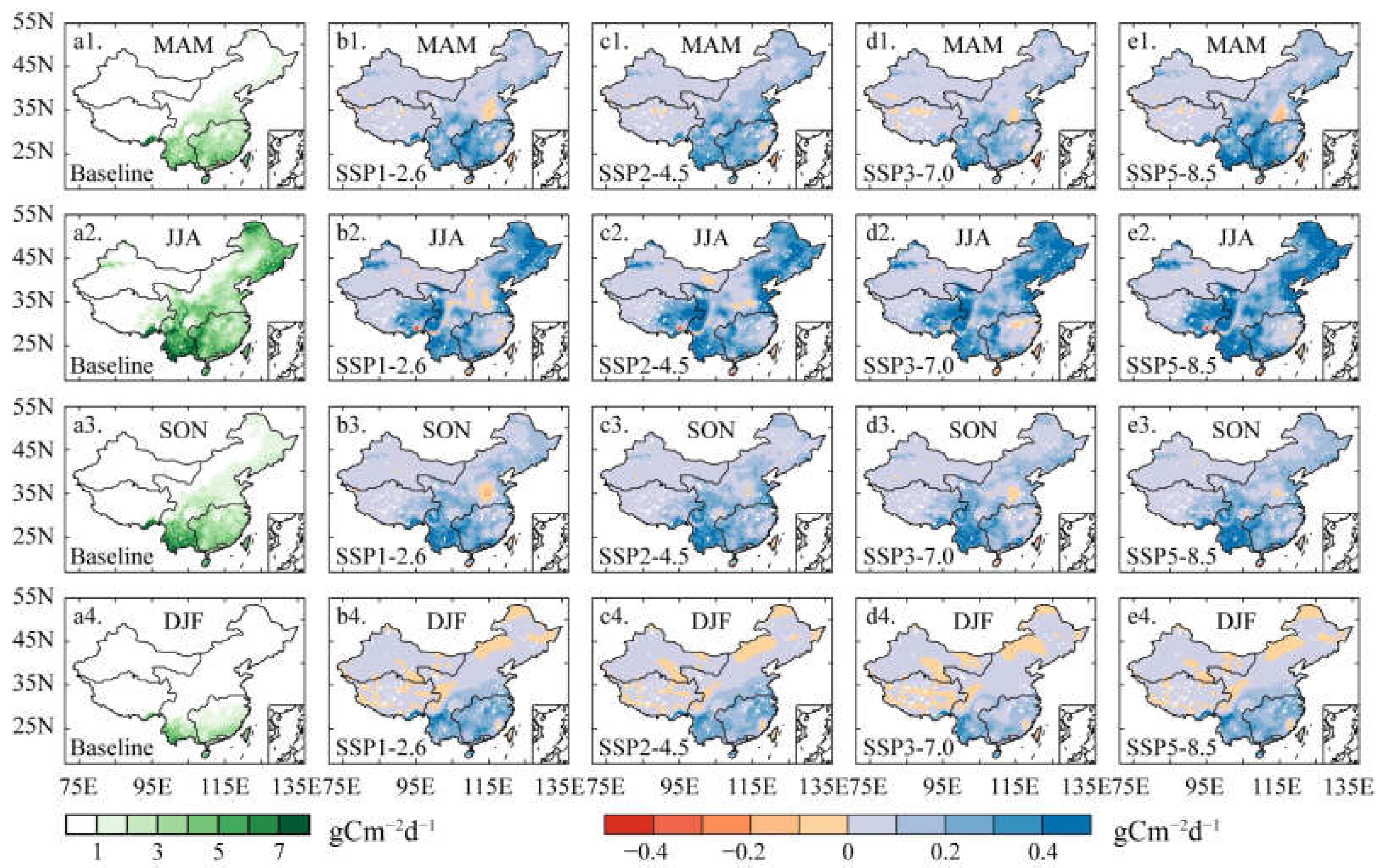
To explore the difference between the changes in GPP in the near future (2021–2040) and the far future (2071–2100), the spatial distribution of the multi-year mean of GPP in each season under different climate scenarios in historical baseline, near, and far future is described in Figure 10 and Figure S2, respectively. Among them, the distributions under different scenarios in the future describe the change in the multi-year mean compared with that during baseline. The positive value represents the increase in GPP, while the negative one represents the decrease. Figure 10a1–a4 shows that the spatial distribution of the mean annual GPP in each season of the baseline GPP increased significantly in the four seasons compared with the seasonal average over the period 1850–2014 (Figure 8). In spring, the average annual GPP greater than 2 gCm−2d−1 occupied 22.93% of the region, concentrated in the south of 30° N. In summer, the area with an annual average GPP of more than 2 gCm−2d−1 doubled compared with spring, reaching 48.97%, with the maximum yearly peak at 14.19 gCm−2d−1. There are similar peaks and spatial distribution in autumn and spring, while it remains almost the same in winter.
There are significant seasonal differences in the variations in GPP based on the historical baseline under multiple scenarios in the near future. In spring, GPP increases in most eastern regions, and rises more with the enhancement of radiation forcing levels. However, GPP decreased significantly in the east of the plain of Henan Province under the high emission scenario. In summer, GPP increased substantially in nearly half of the regions of the country, including the Northeast, North, Southwest, and south of Northwest China. GPP accelerated with the increase in radiation forcing levels, with more than 20% of the regions having values greater than 0.4 gCm−2d−1 under SSP5-8.5. In autumn, it increased significantly in Yunnan, while there was a slight weakening trend in the north of Henan. The spatial characteristics distribution maintains consistency under multiple climate scenarios. Winter is the only season when GPP decreases in a large area. Under the four scenarios, the GPP in 21% of regions is lower than the baseline, mainly distributed in the west, Inner Mongolia, and Heilongjiang. The reduction in GPP is the same under different scenarios. Except for the decrease in GPP in Fujian, it generally increases in the south.
The change in GPP becomes increasingly intense with the enhancement of radiative forcing levels in the far future, as seen from Figure S2. The variations in GPP are studied with the Heihe–Tengchong line as the boundary. In spring, it can be found that GPP increases more as radiative forcing levels are enhanced in the eastern part of the dividing line. The area with an increase of more than 0.8 gCm−2d−1 rises from 0.62% to 23.99%. The change in the west of the boundary is gentle, with an average rise of 0.09 gCm−2d−1. The area of GPP increasing by more than 0.8 gCm−2d−1 expands from 0.62% to 23.99% of the regions. The change in the western part of the dividing line is relatively gentle, with an average increase of 0.09 gCm−2d−1. Summer is the peak photosynthesis season for plants in northern ecosystems compared to other seasons, leading to a more extensive range and broader areas of increase. GPP increases in about 94% of the regions under SSP1-2.6 relative to the baseline. With the enhancement of radiation forcing levels, the rise of GPP in Northeast, North, and the east of Southwest China becomes more and more intense, while that in Henan is turning from decrease to increase. The magnitude of the increase is further accelerated under SSP5-8.5. The reduction in GPP in Henan in autumn only occurs in the low-emission scenario, which differs from spring. In winter, GPP reduces in parts of the west and northeast regions, roughly similar to the scenario in the near future (Figure 10b1–e4). There is a considerable area reduction in GPP in the eastern part of the Qinghai–Tibet Plateau under the SSP1-2.6 scenario. With the increase in radiation forcing levels, the area of GPP reduction gradually decreases. GPP increased south of 30° N, with the maximum increase reaching 2.48 gCm−2d−1 in Yunnan under the SSP5-8.5 scenario. Compared with the near future, GPP growth will be more dramatic in the far future.
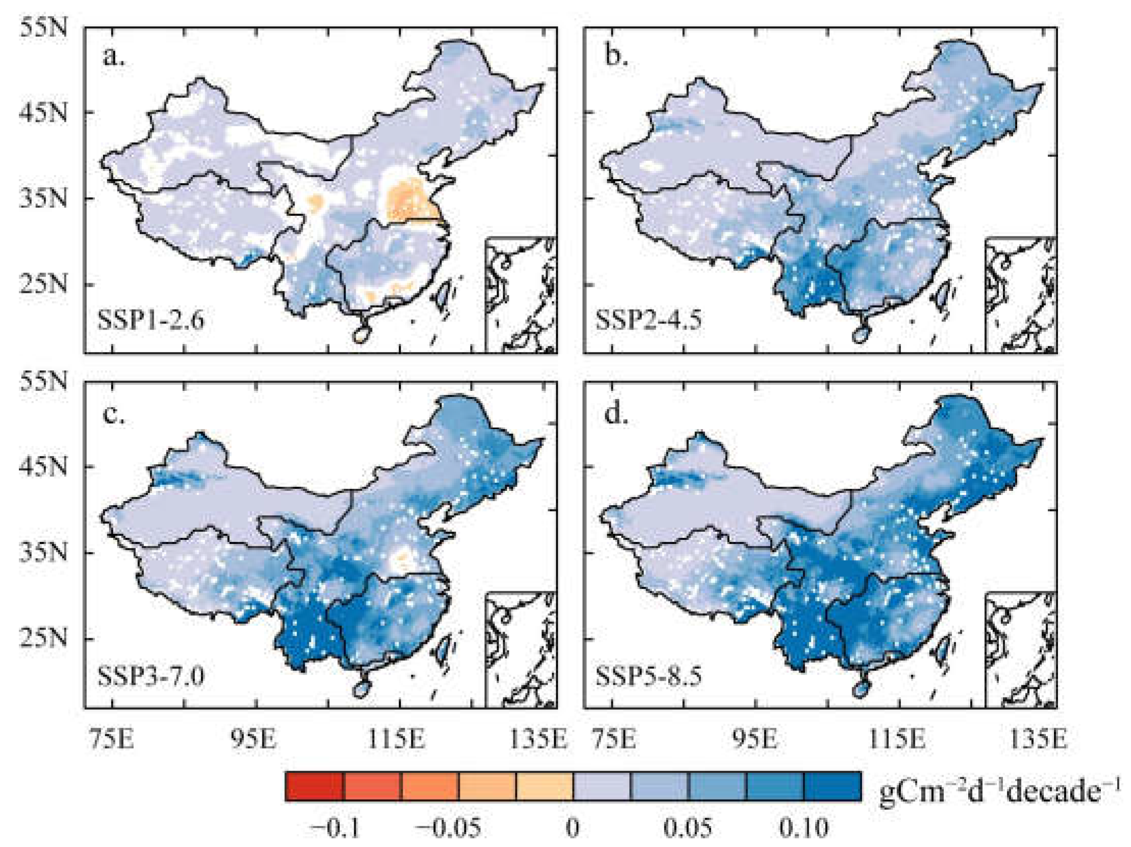
The multi-year variations in GPP in each pixel can better reflect the characteristics of spatial changes in addition to the regional average. Figure 11 describes the spatial distribution of GPP variation trends in China under four scenarios from 2015 to 2100. GPP generally shows an increasing trend in the projection period, with the trend becoming more and more intense as the radiation forcing levels increase. There is no significant change in GPP in the northwest arid regions under different scenarios, which maintains a low growth. A slight decreasing trend can be observed visually at the junction of Shandong, Henan, Jiangsu, and Anhui provinces under the SSP1-2.6 scenario, which is related to the environmental effects of aerosols [66]. The spatial pattern of GPP variations under the medium and high emission scenario is similar, with GPP increasing in each pixel. Likewise, the variation trends become more intense as radiative forcing levels increase. The most significant increase in GPP occurs in Yunnan and Guizhou under SSP2-4.5, SSP3-7.0, and SSP5-8.5. The regions where GPP is more sensitive to radiation forcing levels are concentrated in the southwest, the east of the northwest, and the northeast. GPP increases rapidly as radiative forcing levels increase. It is found that the increase in the high-emission scenario is even four times that of the low-emission scenario.
Considering the characteristics of the future variations in GPP, it is divided into three periods for analysis, including 2021–2040 (near future), 2041–2070 (medium future), and 2071–2100 (far future) due to the long projection period of the merged data. As can be seen from Figure S3, the increasing trend of GPP turns into a decreasing trend as time goes on under the SSP1-2.6 scenario. In the near future, GPP shows a significant increasing trend except for the junction of Shandong, Jiangsu, Henan, and Anhui provinces. In the medium future, the changes in average regional GPP are relatively stable, though there are scattered pixels with increasing and decreasing trends of GPP across the country. In the far future, the regions with reduced trends of GPP nationwide account for about 93% of the country. Under the low emission scenario, the air temperature rises first and remains stable in the far future, while the carbon dioxide emissions begin to decrease in 2020 [67]. This shows that GPP is greatly affected by air temperature. The amount of carbon dioxide directly affects vegetation’s carbon sequestration when the temperature is stable, leading to GPP decline. GPP increases in the near future under the SSP2-4.5 scenario; however, the variation trends slow down over time. Under SSP3-7.0 and SSP5-8.5 scenarios, GPP increased over time in all regions, with the trends strengthening gradually.
4. Discussion
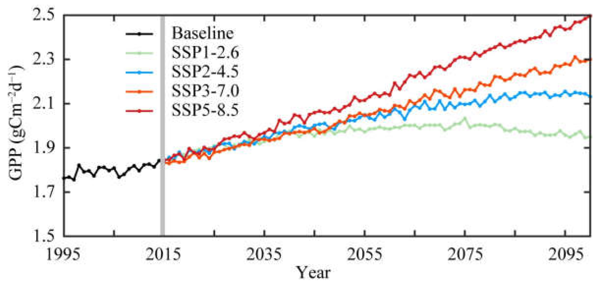
It can be seen from Figure 10 and Figure S2 that the variations in GPP in the north and south of China are opposite in winter while increasing in all regions in spring, summer, and autumn. However, this cannot reflect the impact of the reduction in winter on the change in the average GPP across the country. Therefore, Figure 12 shows the inter-annual changes in GPP in China under the historical baseline and different scenarios in the future. The thick grey line represents the line between the baseline and the future. GPP shows an increasing trend from 1.76 gCm−2d−1 to 1.84 gCm−2d−1 from 1995 to 2014. It may result from a combination of factors such as appropriate climate change, the fertilization effect of CO2, nitrogen deposition, and human activities such as afforestation and agricultural irrigation [68,69,70,71]. From 2015 to 2035, GPP increases steadily yearly with similar increasing trends under the four scenarios. From 2036, the difference in the variations in GPP in the four scenarios is noticeable. Among them, the variation speed of GPP is the fastest under SSP5-8.5, with the average reaching 2.49 gCm−2d−1 at the end of the 21st century. The second fastest occurs under SSP3-7.0, which is slightly slower than that of the high-emission scenario. The annual average is roughly the same before 2055 as under SSP2-4.5. However, the gap between the two scenarios gradually increases from 2067, when the growth rate under SSP2-4.5 slows down. From 2081 to 2100, it is almost stable and begins declining slowly in 2097. Among the four scenarios, GPP decreases significantly only in the SSP1-2.6 scenario. Although there is a decreasing trend at the end of the century under the SSP2-4.5 scenario (Figure 12), GPP shows an overall increasing trend in each pixel over the period 2015–2100 (Figure 11b). More specifically, it keeps increasing, as do the other three scenarios in the near future, followed by a slight fluctuation around 1.96 gCm−2d−1 for a long time in the medium term. It is worth noting that GPP declines significantly in the far future, especially from 2075 onwards. Meteorological factors are the dominant factors in the interannual variation in global GPP. In the context of climate warming, the frequent occurrence of extreme events such as high temperatures and droughts is expected to impact vegetation growth, leading to fluctuations in ecosystem GPP. According to the definition of severe climate, the Intergovernmental Panel on Climate Change [72] pointed out that climate change has led to changes in the frequency, intensity, spatial scope, duration, and time of extreme climate, which may have an unprecedented impact on the terrestrial carbon cycle. In addition, due to global warming, climate change is expected to further increase the frequency, persistence, and intensity of extreme weather in the mid to late 21st century [73,74,75], making the impact of future climate change on terrestrial ecosystems even more uncertain [76,77].
Large-scale studies using merged GPP can reduce the uncertainty of terrestrial ecosystem carbon cycle research. However, the merging process will also introduce certain uncertainties, mainly affected by input errors, scale effects, and merging algorithms. Input errors are caused by the CMIP6 datasets, GLASS GPP, and flux tower observation GPP. Although model simulation provides an essential research tool for the carbon cycle of large-scale terrestrial ecosystems, there are still significant differences in the simulation results of the models at regional and global scales due to the differences in the structure, parameter settings, input data, and spatial resolution of each CMIP6 model. Schaefer et al. [5] compared GPP simulation differences in North America across 26 models to explore the responses of different model structures and environmental factors to simulations based on data from 39 flux stations. Zhang et al. [78] studied the impact of different parameter settings and meteorological data in the CEVSA2 model on the GPP simulation results in the Changbai Mountain region of China from 2003 to 2005, indicating that the GPP difference caused by parameter setting in the model is 5% to 8%. The reference data GLASS GPP is generated by integrating multiple algorithms using the Bayesian integration method, reducing the uncertainty of a single algorithm. However, there are differences in spatial scales between ground and satellite data, and the algorithm fails to distinguish potential differences in photosynthesis between C3 and C4 crops. In addition, the problem of mixed pixels can also affect the accuracy of GLASS GPP estimation [79]. The GPP observed by the flux tower is considered the benchmark, while the high heterogeneity of the ground can also make the representativeness of the flux station data poor. Therefore, significant uncertainties in the GPP benchmark lead to a lack of consensus on the global GPP distribution [15,80]. Chen et al. [81] showed that the flux-tower-estimated GPP represents 50% to 60% of the actual situation in the case of surface heterogeneity. There is still a problem of insufficient spatial representation compared to the range of flux contribution areas assumed by eddy covariance.
The mismatch between the spatial resolution of the model and the floor area of the flux tower causes the uncertainty imposed by scale effects. Even with the same model and source of input data, the simulation results may still be different due to spatial heterogeneity caused by different spatial resolutions [1]. At the regional scale, improving spatial resolution can reduce the uncertainty of GPP simulation [82]. However, in practical applications, models often need to simulate large-scale and long-time series data. When considering factors such as simulation time, data storage capacity, and analysis difficulty, they often reduce the spatial resolution to improve simulation efficiency. In GPP estimation at different spatial scales, there will be different judgments on the coverage type, leading to incorrect maximum light energy utilization, further resulting in errors. In mid- and low-resolution GPP remote sensing products, most of the pixels under heterogeneous ground surfaces are mixed. For example, there is a significant difference between MODIS surface coverage with 1 km and global 30 m resolution. At different scales, heterogeneity characteristics have an important impact on surface vegetation parameter characteristics [83]. Taking the mixed pixel of forest and grassland as an example, there is a significant difference in the a priori maximum light energy utilization rate between the two types. It may bring about significant errors using a single type of maximum weak energy utilization rate to replace pixel values. Wang et al. [1] discussed the impact of two spatial resolutions of 1 km and 8 km input data on GPP simulation, with the results showing that the difference was mainly due to the difference in LAI caused by mixed pixels within the range of 8km. The difference in simulation results with different spatial resolutions at forest stations was more significant than that at grassland stations. Therefore, it is feasible to appropriately reduce spatial resolution to improve the model’s simulation efficiency. However, it is necessary to minimize the error of low spatial resolution in the GPP simulation of forest ecosystems and growing seasons.
In the long sequence data merging, considering time information can effectively enhance model learning capabilities and improve the quality of merged data, which helps to reduce the data uncertainty in the projection period. Since the deep learning merging model focuses more on spatial features and no individual modules can capture temporal characteristics, the temporal information is not fully utilized. In addition, there are other factors contributing to uncertainties. For example, complex vegetation structures, significant dry and wet seasons, and cloud cover can also bring uncertainties [84]. In highly productive regions, methods based on optical remote sensing often underestimate GPP due to the saturation of reflectance measurements in high-density canopy [85]. In addition, optical remote sensing is strongly affected by cloud cover, resulting in data gaps and high uncertainty in areas with frequent cloud cover and high GPP, such as tropical forests [16].
5. Conclusions
In this study, a GPP-merged dataset with high resolution in China has been developed using the deep learning method. It combines the advantages of 23 CMIP6 GPP datasets without relying on any prior knowledge. The lower resolution of the multi-model data has been improved to 0.25° of the merged GPP. From the perspective of evaluation indicators, the performance of merged data is superior to the others in all aspects. In China, the error has been kept at a low level. The merged dataset has significantly improved in temporal and spatial dimensions compared with every single model and the multi-model mean. The merged data are closer to the actual value than the multi-model mean according to the fluxnet data. The merged data greatly reduce the uncertainties and improve the reliability of GPP estimation in the projection period. A further analysis of the spatiotemporal change pattern of GPP in China has resulted in the following findings.
During the baseline, GPP is the highest in summer, followed by spring and autumn, and the lowest in winter due to the combined effects of factors such as the monsoon climate and vegetation types. GPP exhibits significant spatial heterogeneity due to differences in topography, vegetation types, and hydrothermal conditions in different regions. Generally, GPP increases gradually from the northwest inland to the southeast coast. GPP in the southern part of Yunnan remains high in winter. According to the long-term variation trends, GPP is increasing in most regions of China. It is worth noting that the characteristics of the decrease in the southern coastal areas and Inner Mongolia are not captured by the multi-model ensemble mean; however, they are captured by the merged GPP. There are seasonal differences in the variations in GPP relative to the baseline under different scenarios in the future projection period, while the variations are almost the same across different scenarios in the near future. In summer, GPP increased rapidly with the increase in radiation forcing levels. In winter, GPP decreases in a large region mainly distributed in the west, Inner Mongolia, and Heilongjiang. The long-term variation trends of GPP in China under different scenarios are significantly different. The growth rate of GPP has reached the maximum under the SSP5-8.5 scenario since 2036. The increasing trend becomes slightly slower under the SSP3-7.0 scenario than under the high-emission scenario. Furthermore, GPP decreased significantly under the SSP1-2.6 scenario. The annual GPP in each pixel in China shows an increasing trend, which is more intense with the increase in radiation forcing levels. GPP changes from increasing to decreasing over time, since GPP is affected by temperature and carbon dioxide under the SSP1-2.6 scenario. Under the SSP2-4.5 scenario, GPP will increase in the near future; however, the trend will slow down as time goes by. Under the SSP3-7.0 and SSP5-8.5 scenarios, GPP increases with time; the increasing trend rises gradually.
Supplementary Materials
The following supporting information can be downloaded at https://www.mdpi.com/article/10.3390/f14061201/s1, Figure S1: The probability density distribution of GLASS GPP during 1982–2014, Figure S2: Spatial distribution of the multi-annual mean GPP in far future (2071–2100) relative to baseline under (a1–a4) SSP 1-2.6, (b1–b4) SSP2-4.5, (c1–c4) SSP 3-7.0, (d1–d4), and SSP 5-8.5 in (a1–d1) spring, (a2–d2) summer, (a3–d3) autumn, and (a4–d4) winter, Figure S3: Spatial distribution of the variation trends of annual average GPP under four climate scenarios in the near, middle, and far future, with the dot indicating passing significance test at 5% level.
Author Contributions
Conceptualization, J.L. and G.W.; methodology, J.L. and D.F.; software, J.L. and D.F.; validation, D.F. and I.K.N.; formal analysis, J.L.; investigation, J.L.; resources, D.F.; data curation, I.K.N.; writing—original draft preparation, J.L.; writing—review and editing, J.L. and G.W.; visualization, J.L.; supervision, G.W.; project administration, J.L. and G.W.; funding acquisition, J.L. and G.W. All authors have read and agreed to the published version of the manuscript.
Funding
This research was funded by China Meteorological Administration Innovation Development Project (CXFZ2023J071) and the Wuxi University Research Start-up Fund for Introduced Talents (2023r041).
Data Availability Statement
Data are available from https://doi.org/10.6084/m9.figshare.22004504.v1 (accessed on 23 April 2023).
Conflicts of Interest
The authors declare no conflict of interest. The funders had no role in the design of the study; in the collection, analyses, or interpretation of data; in the writing of the manuscript; or in the decision to publish the results.
References
- Wang, M.; Zhou, L.; Wang, S.; Wang, X.; Sun, L. An analysis of the Gross Primary Productivity simulation difference resulting from the spatial resolution. Geogr. Res. 2016, 35, 617–626. [Google Scholar]
- Zhang, X.; Wang, H.; Yan, H.; Ai, J. Analysis of spatio-temporal changes of gross primary productivity in China from 2001 to 2018 based on Remote Sensing. Acta Ecol. Sin. 2021, 41, 6351–6362. [Google Scholar]
- Ito, A.; Inatomi, M.; Huntzinger, D.N.; Schwalm, C.; Michalak, A.M.; Cook, R.; King, A.W.; Mao, J.; Wei, Y.; Post, W.M.; et al. Decadal trends in the seasonal-cycle amplitude of terrestrial CO2 exchange resulting from the ensemble of terrestrial biosphere models. Tellus B Chem. Phys. Meteorol. 2016, 68, 28968. [Google Scholar] [CrossRef]
- Chen, M.; Rafique, R.; Asrar, G.R.; Bond-Lamberty, B.; Ciais, P.; Zhao, F.; Reyer, C.P.O.; Ostberg, S.; Chang, J.; Ito, A.; et al. Regional contribution to variability and trends of global gross primary productivity. Environ. Res. Lett. 2017, 12, 105005. [Google Scholar] [CrossRef]
- Schaefer, K.; Schwalm, C.R.; Williams, C.; Arain, M.A.; Barr, A.; Chen, J.M.; Davis, K.J.; Dimitrov, D.; Hilton, T.W.; Hollinger, D.Y.; et al. A model-data comparison of gross primary productivity: Results from the North American Carbon Program site synthesis. J. Geophys. Res. Biogeosci. 2012, 117, G03010. [Google Scholar] [CrossRef] [Green Version]
- Friedlingstein, P.; O’Sullivan, M.; Jones, M.W.; Andrew, R.M.; Hauck, J.; Olsen, A.; Peters, G.P.; Peters, W.; Pongratz, J.; Sitch, S.; et al. Global Carbon Budget 2020. Earth Syst. Sci. Data 2020, 12, 3269–3340. [Google Scholar] [CrossRef]
- Damm, A.; Elbers, J.A.N.; Erler, A.; Gioli, B.; Hamdi, K.; Hutjes, R.; Kosvancova, M.; Meroni, M.; Miglietta, F.; Moersch, A.; et al. Remote sensing of sun-induced fluorescence to improve modeling of diurnal courses of gross primary production (GPP). Glob. Chang. Biol. 2010, 16, 171–186. [Google Scholar] [CrossRef] [Green Version]
- Guo, L.; Gao, J.; Ma, S.; Chang, Q.; Zhang, L.; Wang, S.; Zou, Y.; Wu, S.; Xiao, X. Impact of spring phenology variation on GPP and its lag feedback for winter wheat over the North China Plain. Sci. Total Environ. 2020, 725, 138342. [Google Scholar] [CrossRef] [PubMed]
- Wang, S.; Quan, Q.; Meng, C.; Chen, W.; Luo, Y.; Niu, S.; Yang, Y. Experimental warming shifts coupling of carbon and nitrogen cycles in an alpine meadow. J. Plant Ecol. 2021, 14, 541–554. [Google Scholar] [CrossRef]
- Zhang, Z.; Zhang, Y.; Porcar-Castell, A.; Joiner, J.; Guanter, L.; Yang, X.; Migliavacca, M.; Ju, W.; Sun, Z.; Chen, S.; et al. Reduction of structural impacts and distinction of photosynthetic pathways in a global estimation of GPP from space-borne solar-induced chlorophyll fluorescence. Remote Sens. Environ. 2020, 240, 111722. [Google Scholar] [CrossRef]
- Cheng, Y.-B.; Zhang, Q.; Lyapustin, A.I.; Wang, Y.; Middleton, E.M. Impacts of light use efficiency and fPAR parameterization on gross primary production modeling. Agric. For. Meteorol. 2014, 189–190, 187–197. [Google Scholar] [CrossRef]
- Baldocchi, D.; Ryu, Y.; Keenan, T. Terrestrial Carbon Cycle Variability. F1000research 2016, 5, 2371. [Google Scholar] [CrossRef] [Green Version]
- Nemani, R.R.; Keeling, C.D.; Hashimoto, H.; Jolly, W.M.; Piper, S.C.; Tucker, C.J.; Myneni, R.B.; Running, S.W. Climate-driven increases in global terrestrial net primary production from 1982 to 1999. Science 2003, 300, 1560–1563. [Google Scholar] [CrossRef] [Green Version]
- Speckman, H.N.; Frank, J.M.; Bradford, J.B.; Miles, B.L.; Massman, W.J.; Parton, W.J.; Ryan, M.G. Forest ecosystem respiration estimated from eddy covariance and chamber measurements under high turbulence and substantial tree mortality from bark beetles. Glob. Chang. Biol. 2015, 21, 708–721. [Google Scholar] [CrossRef]
- Anav, A.; Friedlingstein, P.; Beer, C.; Ciais, P.; Harper, A.; Jones, C.; Murray-Tortarolo, G.; Papale, D.; Parazoo, N.C.; Peylin, P.; et al. Spatiotemporal patterns of terrestrial gross primary production: A review. Rev. Geophys. 2015, 53, 785–818. [Google Scholar] [CrossRef] [Green Version]
- Wild, B.; Teubner, I.; Moesinger, L.; Zotta, R.-M.; Forkel, M.; van der Schalie, R.; Sitch, S.; Dorigo, W. VODCA2GPP—A new, global, long-term (1988–2020) gross primary production dataset from microwave remote sensing. Earth Syst. Sci. Data 2022, 14, 1063–1085. [Google Scholar] [CrossRef]
- Chen, Y.; Gu, H.; Wang, M.; Gu, Q.; Ding, Z.; Ma, M.; Liu, R.; Tang, X. Contrasting Performance of the Remotely-Derived GPP Products over Different Climate Zones across China. Remote Sens. 2019, 11, 1855. [Google Scholar] [CrossRef] [Green Version]
- Pei, Y.; Dong, J.; Zhang, Y.; Yang, J.; Zhang, Y.; Jiang, C.; Xiao, X. Performance of four state-of-the-art GPP products (VPM, MOD17, BESS and PML) for grasslands in drought years. Ecol. Inform. 2020, 56, 101052. [Google Scholar] [CrossRef]
- Zheng, Y.; Shen, R.; Wang, Y.; Li, X.; Liu, S.; Liang, S.; Chen, J.M.; Ju, W.; Zhang, L.; Yuan, W. Improved estimate of global gross primary production for reproducing its long-term variation, 1982–2017. Earth Syst. Sci. Data 2020, 12, 2725–2746. [Google Scholar] [CrossRef]
- Gu, Y.; Wylie, B.K.; Howard, D.M.; Phuyal, K.P.; Ji, L. NDVI saturation adjustment: A new approach for improving cropland performance estimates in the Greater Platte River Basin, USA. Ecol. Indic. 2013, 30, 1–6. [Google Scholar] [CrossRef]
- Lawrence, D.M.; Fisher, R.A.; Koven, C.D.; Oleson, K.W.; Swenson, S.C.; Bonan, G.; Collier, N.; Ghimire, B.; van Kampenhout, L.; Kennedy, D.; et al. The Community Land Model Version 5: Description of New Features, Benchmarking, and Impact of Forcing Uncertainty. J. Adv. Model. Earth Syst. 2019, 11, 4245–4287. [Google Scholar] [CrossRef] [Green Version]
- Jung, M.; Schwalm, C.; Migliavacca, M.; Walther, S.; Camps-Valls, G.; Koirala, S.; Anthoni, P.; Besnard, S.; Bodesheim, P.; Carvalhais, N.; et al. Scaling carbon fluxes from eddy covariance sites to globe: Synthesis and evaluation of the FLUXCOM approach. Biogeosciences 2020, 17, 1343–1365. [Google Scholar] [CrossRef] [Green Version]
- Jung, M.; Reichstein, M.; Bondeau, A. Towards global empirical upscaling of FLUXNET eddy covariance observations: Validation of a model tree ensemble approach using a biosphere model. Biogeosciences 2009, 6, 2001–2013. [Google Scholar] [CrossRef] [Green Version]
- Jung, M.; Reichstein, M.; Margolis, H.A.; Cescatti, A.; Richardson, A.D.; Arain, M.A.; Arneth, A.; Bernhofer, C.; Bonal, D.; Chen, J.; et al. Global patterns of land-atmosphere fluxes of carbon dioxide, latent heat, and sensible heat derived from eddy covariance, satellite, and meteorological observations. J. Geophys. Res. 2011, 116, 1–16. [Google Scholar] [CrossRef] [Green Version]
- Stocker, B.D.; Zscheischler, J.; Keenan, T.F.; Prentice, I.C.; Penuelas, J.; Seneviratne, S.I. Quantifying soil moisture impacts on light use efficiency across biomes. New Phytol. 2018, 218, 1430–1449. [Google Scholar] [CrossRef] [PubMed] [Green Version]
- Tramontana, G.; Ichii, K.; Camps-Valls, G.; Tomelleri, E.; Papale, D. Uncertainty analysis of gross primary production upscaling using Random Forests, remote sensing and eddy covariance data. Remote Sens. Environ. 2015, 168, 360–373. [Google Scholar] [CrossRef]
- Tramontana, G.; Jung, M.; Schwalm, C.R.; Ichii, K.; Camps-Valls, G.; Ráduly, B.; Reichstein, M.; Arain, M.A.; Cescatti, A.; Kiely, G.; et al. Predicting carbon dioxide and energy fluxes across global FLUXNET sites with regression algorithms. Biogeosciences 2016, 13, 4291–4313. [Google Scholar] [CrossRef] [Green Version]
- Wei, S.; Yi, C.; Fang, W.; Hendrey, G. A global study of GPP focusing on light-use efficiency in a random forest regression model. Ecosphere 2017, 8, e01724. [Google Scholar] [CrossRef]
- O’Sullivan, M.; Smith, W.K.; Sitch, S.; Friedlingstein, P.; Arora, V.K.; Haverd, V.; Jain, A.K.; Kato, E.; Kautz, M.; Lombardozzi, D.; et al. Climate-Driven Variability and Trends in Plant Productivity Over Recent Decades Based on Three Global Products. Glob. Biogeochem. Cycles 2020, 34, e2020GB006613. [Google Scholar] [CrossRef]
- Gilabert, M.; Sánchez-Ruiz, S.; Moreno, Á. Annual Gross Primary Production from Vegetation Indices: A Theoretically Sound Approach. Remote Sens. 2017, 9, 193. [Google Scholar] [CrossRef] [Green Version]
- Alemohammad, S.H.; Fang, B.; Konings, A.G.; Aires, F.; Green, J.K.; Kolassa, J.; Miralles, D.; Prigent, C.; Gentine, P. Water, Energy, and Carbon with Artificial Neural Networks (WECANN): A statistically-based estimate of global surface turbulent fluxes and gross primary productivity using solar-induced fluorescence. Biogeosciences 2017, 14, 4101–4124. [Google Scholar] [CrossRef] [PubMed] [Green Version]
- Chen, J.M.; Mo, G.; Pisek, J.; Liu, J.; Deng, F.; Ishizawa, M.; Chan, D. Effects of foliage clumping on the estimation of global terrestrial gross primary productivity. Glob. Biogeochem. Cycles 2012, 26, 1–18. [Google Scholar] [CrossRef] [Green Version]
- Ryu, Y.; Baldocchi, D.D.; Kobayashi, H.; van Ingen, C.; Li, J.; Black, T.A.; Beringer, J.; van Gorsel, E.; Knohl, A.; Law, B.E.; et al. Integration of MODIS land and atmosphere products with a coupled-process model to estimate gross primary productivity and evapotranspiration from 1 km to global scales. Glob. Biogeochem. Cycles 2011, 25, GB4017. [Google Scholar] [CrossRef] [Green Version]
- Yuan, W.; Liu, S.; Liang, S.; Tan, Z.; Liu, H.; Young, C. Estimations of Evapotranspiration and Water Balance with Uncertainty over the Yukon River Basin. Water Resour. Manag. 2012, 26, 2147–2157. [Google Scholar] [CrossRef]
- Yuan, W.; Liu, S.; Dong, W.; Liang, S.; Zhao, S.; Chen, J.; Xu, W.; Li, X.; Barr, A.; Andrew Black, T.; et al. Differentiating moss from higher plants is critical in studying the carbon cycle of the boreal biome. Nat. Commun. 2014, 5, 4270. [Google Scholar] [CrossRef] [Green Version]
- Dunne, J.P.; John, J.G.; Adcroft, A.J.; Griffies, S.M.; Hallberg, R.W.; Shevliakova, E.; Stouffer, R.J.; Cooke, W.; Dunne, K.A.; Harrison, M.J.; et al. GFDL’s ESM2 Global Coupled Climate–Carbon Earth System Models. Part I: Physical Formulation and Baseline Simulation Characteristics. J. Clim. 2012, 25, 6646–6665. [Google Scholar] [CrossRef] [Green Version]
- Gent, P.R.; Danabasoglu, G.; Donner, L.J.; Holland, M.M.; Hunke, E.C.; Jayne, S.R.; Lawrence, D.M.; Neale, R.B.; Rasch, P.J.; Vertenstein, M.; et al. The Community Climate System Model Version 4. J. Clim. 2011, 24, 4973–4991. [Google Scholar] [CrossRef] [Green Version]
- Sun, Z.; Wang, X.; Zhang, X.; Tani, H.; Guo, E.; Yin, S.; Zhang, T. Evaluating and comparing remote sensing terrestrial GPP models for their response to climate variability and CO2 trends. Sci. Total Environ. 2019, 668, 696–713. [Google Scholar] [CrossRef]
- Bentsen, M.; Bethke, I.; Debernard, J.B.; Iversen, T.; Kirkevåg, A.; Seland, Ø.; Drange, H.; Roelandt, C.; Seierstad, I.A.; Hoose, C.; et al. The Norwegian Earth System Model, NorESM1-M—Part 1: Description and basic evaluation of the physical climate. Geosci. Model Dev. 2013, 6, 687–720. [Google Scholar] [CrossRef] [Green Version]
- Williams, M.; Richardson, A.D.; Reichstein, M.; Stoy, P.C.; Peylin, P.; Verbeeck, H.; Carvalhais, N.; Jung, M.; Hollinger, D.Y.; Kattge, J.; et al. Improving land surface models with FLUXNET data. Biogeosciences 2009, 6, 1341–1359. [Google Scholar] [CrossRef] [Green Version]
- Beer, C.; Reichstein, M.; Tomelleri, E.; Ciais, P.; Jung, M.; Carvalhais, N.; Rodenbeck, C.; Arain, M.A.; Baldocchi, D.; Bonan, G.B.; et al. Terrestrial gross carbon dioxide uptake: Global distribution and covariation with climate. Science 2010, 329, 834–838. [Google Scholar] [CrossRef] [Green Version]
- Bo, Y.; Li, X.; Liu, K.; Wang, S.; Zhang, H.; Gao, X.; Zhang, X. Three Decades of Gross Primary Production (GPP) in China: Variations, Trends, Attributions, and Prediction Inferred from Multiple Datasets and Time Series Modeling. Remote Sens. 2022, 14, 2564. [Google Scholar] [CrossRef]
- Zhang, Y.; Ye, A. Would the obtainable gross primary productivity (GPP) products stand up? A critical assessment of 45 global GPP products. Sci. Total Environ. 2021, 783, 146965. [Google Scholar] [PubMed]
- Song, L.; Li, Y.; Ren, Y.; Wu, X.; Guo, B.; Tang, X.; Shi, W.; Ma, M.; Han, X.; Zhao, L. Divergent vegetation responses to extreme spring and summer droughts in Southwestern China. Agric. For. Meteorol. 2019, 279, 107703. [Google Scholar] [CrossRef]
- Yuan, W.; Liu, S.; Yu, G.; Bonnefond, J.-M.; Chen, J.; Davis, K.; Desai, A.R.; Goldstein, A.H.; Gianelle, D.; Rossi, F.; et al. Global estimates of evapotranspiration and gross primary production based on MODIS and global meteorology data. Remote Sens. Environ. 2010, 114, 1416–1431. [Google Scholar] [CrossRef] [Green Version]
- Alexandrov, G.A. CMIP6 simulations of GPP growth satisfy the constraint imposed by increasing CO2 seasonal-cycle amplitude. IOP Conf. Ser. Earth Environ. Sci. 2020, 606, 012003. [Google Scholar] [CrossRef]
- Eyring, V.; Cox, P.M.; Flato, G.M.; Gleckler, P.J.; Abramowitz, G.; Caldwell, P.; Collins, W.D.; Gier, B.K.; Hall, A.D.; Hoffman, F.M.; et al. Taking climate model evaluation to the next level. Nat. Clim. Chang. 2019, 9, 102–110. [Google Scholar] [CrossRef] [Green Version]
- Ichii, K.; Suzuki, T.; Kato, T.; Ito, A.; Hajima, T.; Ueyama, M.; Sasai, T.; Hirata, R.; Saigusa, N.; Ohtani, Y.; et al. Multi-model analysis of terrestrial carbon cycles in Japan: Limitations and implications of model calibration using eddy flux observations. Biogeosciences 2010, 7, 2061–2080. [Google Scholar] [CrossRef] [Green Version]
- Knutti, R.; Furrer, R.; Tebaldi, C.; Cermak, J.; Meehl, G.A. Challenges in Combining Projections from Multiple Climate Models. J. Clim. 2010, 23, 2739–2758. [Google Scholar] [CrossRef] [Green Version]
- Ershadi, A.; McCabe, M.F.; Evans, J.P.; Chaney, N.W.; Wood, E.F. Multi-site evaluation of terrestrial evaporation models using FLUXNET data. Agric. For. Meteorol. 2014, 187, 46–61. [Google Scholar] [CrossRef]
- Dong, C.; Loy, C.C.; Tang, X. Accelerating the Super-Resolution Convolutional Neural Network; Springer International Publishing: Cham, Germany, 2016. [Google Scholar]
- Liu, Y.; Ganguly, A.R.; Dy, J. Climate Downscaling Using YNet: A Deep Convolutional Network with Skip Connections and Fusion. In Proceedings of the 26th ACM SIGKDD International Conference on Knowledge Discovery & Data Mining, Virtual Event, CA, USA, 6–10 July 2020; Association for Computing Machinery: Virtual Event, CA, USA, 2020; pp. 3145–3153. [Google Scholar]
- Feng, D.; Wang, G.; Wei, X.; Amankwah, S.O.Y.; Hu, Y.; Luo, Z.; Hagan, D.F.T.; Ullah, W. Merging and Downscaling Soil Moisture Data From CMIP6 Projections Using Deep Learning Method. Front. Environ. Sci. 2022, 10, 425. [Google Scholar] [CrossRef]
- Cao, Y.J.; Song, Z.H.; Wu, Z.T.; Du, Z.Q. Spatio-temporal dynamics of gross primary productivity in China from 1982 to 2017 based on different datasets. Chin. J. Appl. Ecol. 2022, 33, 2644–2652. [Google Scholar]
- Odena, A.; Dumoulin, V.; Olah, C. Deconvolution and Checkerboard Artifacts. Distill 2016, 1, e3. [Google Scholar] [CrossRef]
- Zan, M.; Zhou, Y.; Ju, W.; Zhang, Y.; Zhang, L.; Liu, Y. Performance of a two-leaf light use efficiency model for mapping gross primary productivity against remotely sensed sun-induced chlorophyll fluorescence data. Sci. Total Environ. 2018, 613–614, 977–989. [Google Scholar] [CrossRef] [PubMed]
- Jia, B.; Luo, X.; Cai, X.; Jain, A.; Huntzinger, D.N.; Xie, Z.; Zeng, N.; Mao, J.; Shi, X.; Ito, A.; et al. Impacts of land use change and elevated CO2 on the interannual variations and seasonal cycles of gross primary productivity in China. Earth Syst. Dyn. 2020, 11, 235–249. [Google Scholar] [CrossRef] [Green Version]
- Li, X.; Liang, S.; Yu, G.; Yuan, W.; Cheng, X.; Xia, J.; Zhao, T.; Feng, J.; Ma, Z.; Ma, M.; et al. Estimation of gross primary production over the terrestrial ecosystems in China. Ecol. Modell. 2013, 261–262, 80–92. [Google Scholar] [CrossRef]
- Yan, H.; Wang, S.Q.; Wang, J.B.; Cao, Y.; Xu, L.L.; Wu, M.X.; Cheng, L.; Mao, L.X.; Zhao, F.H.; Zhang, X.Z.; et al. Multi-model analysis of climate impacts on plant photosynthesis in China during 2000–2015. Int. J. Climatol. 2019, 39, 5539–5555. [Google Scholar] [CrossRef]
- Chen, X.; Fu, B.; Shi, P.; Guo, Q. Vegetation dynamics in response to climate change in Tianshan, Central Asia from 2000 to 2016. Arid Land Geogr. 2019, 42, 162–171. [Google Scholar]
- Zhang, Y.; Zhang, C.; Wang, Z.; Chen, Y.; Gang, C.; An, R.; Li, J. Vegetation dynamics and its driving forces from climate change and human activities in the Three-River Source Region, China from 1982 to 2012. Sci. Total Environ. 2016, 563–564, 210–220. [Google Scholar] [CrossRef]
- Luo, L.; Ma, W.; Zhuang, Y.; Zhang, Y.; Yi, S.; Xu, J.; Long, Y.; Ma, D.; Zhang, Z. The impacts of climate change and human activities on alpine vegetation and permafrost in the Qinghai-Tibet Engineering Corridor. Ecol. Indic. 2018, 93, 24–35. [Google Scholar] [CrossRef]
- Jiang, Y.; Guo, J.; Peng, Q.; Guan, Y.; Zhang, Y.; Zhang, R. The effects of climate factors and human activities on net primary productivity in Xinjiang. Int. J. Biometeorol. 2020, 64, 765–777. [Google Scholar] [CrossRef]
- Jia, J.; Hu, Z. Spatial and Temporal Features and Trend of Different Level Heat Waves Over China. Adv. Earth Sci. 2017, 32, 546–559. [Google Scholar]
- Ye, D.; Yin, J.; Chen, Z.; Zheng, Y.; Wu, R. Spatiotemporal Change Characteristics of Summer Heatwaves in China in 1961–2010. Clim. Chang. Res. 2013, 9, 15–20. [Google Scholar]
- Gao, M. Environmental Effect Condition (Air Temperature) of Aerosols on Gross Primary Productivity of Vegetation. Int. J. Ecol. 2020, 09, 210–222. [Google Scholar] [CrossRef]
- Zhou, B.; Qian, J. Changes of weather and climate extremes in the IPCC AR6. Clim. Chang. Res. 2021, 17, 713–718. [Google Scholar]
- Piao, S.; Sitch, S.; Ciais, P.; Friedlingstein, P.; Peylin, P.; Wang, X.; Ahlstrom, A.; Anav, A.; Canadell, J.G.; Cong, N.; et al. Evaluation of terrestrial carbon cycle models for their response to climate variability and to CO2 trends. Glob. Chang. Biol. 2013, 19, 2117–2132. [Google Scholar] [CrossRef] [PubMed] [Green Version]
- Lu, C.; Tian, H.; Liu, M.; Ren, W.; Xu, X.; Chen, G.; Zhang, C. Effect of nitrogen deposition on China’s terrestrial carbon uptake in the context of multifactor environmental changes. Ecol. Appl. 2012, 22, 53–75. [Google Scholar] [CrossRef] [PubMed]
- Ouyang, Z.; Zheng, H.; Xiao, Y.; Polasky, S.; Liu, J.; Xu, W.; Wang, Q.; Zhang, L.; Xiao, Y.; Rao, E.; et al. Improvements in ecosystem services from investments in natural capital. Science 2016, 352, 1455–1459. [Google Scholar] [CrossRef] [PubMed]
- Yuan, W.; Li, X.; Liang, S.; Cui, X.; Dong, W.; Liu, S.; Xia, J.; Chen, Y.; Liu, D.; Zhu, W. Characterization of locations and extents of afforestation from the Grain for Green Project in China. Remote Sens. Lett. 2014, 5, 221–229. [Google Scholar] [CrossRef]
- IPCC. Managing the Risks of Extreme Events and Disasters to Advance Climate Change Adaption; IPCC: Cambridge, UK, 2012; p. 582. [Google Scholar]
- IPCC. Climate Change 2013: The Physical Science Basis. Contribution of Working Group I to the Fifth Assessment Report of the Intergovernmental Panel on Climate Change; IPCC: Cambridge, UK; New York, NY, USA, 2013; p. 1535. [Google Scholar]
- Niu, X.; Wang, S.; Tang, J.; Lee, D.-K.; Gutowski, W.; Dairaku, K.; McGregor, J.; Katzfey, J.; Gao, X.; Wu, J.; et al. Ensemble evaluation and projection of climate extremes in China using RMIP models. Int. J. Climatol. 2018, 38, 2039–2055. [Google Scholar] [CrossRef]
- Sui, Y.; Lang, X.; Jiang, D. Projected signals in climate extremes over China associated with a 2 °C global warming under two RCP scenarios. Int. J. Climatol. 2018, 38, e678–e697. [Google Scholar] [CrossRef]
- Samaniego, L.; Thober, S.; Kumar, R.; Wanders, N.; Rakovec, O.; Pan, M.; Zink, M.; Sheffield, J.; Wood, E.F.; Marx, A. Anthropogenic warming exacerbates European soil moisture droughts. Nat. Clim. Chang. 2018, 8, 421–426. [Google Scholar] [CrossRef] [Green Version]
- Yao, R.; Wang, L.; Huang, X.; Chen, X.; Liu, Z. Increased spatial heterogeneity in vegetation greenness due to vegetation greening in mainland China. Ecol. Indic. 2019, 99, 240–250. [Google Scholar] [CrossRef]
- Zhang, L.; Yu, G.; Gu, F.; He, H.; Zhang, L.; Han, S. Uncertainty analysis of modeled carbon fluxes for a broad-leaved Korean pine mixed forest using a process-based ecosystem model. J. For. Res. 2012, 17, 268–282. [Google Scholar] [CrossRef]
- Yu, T.; Sun, R.; Xiao, Z.; Zhang, Q.; Liu, G.; Cui, T.; Wang, J. Estimation of Global Vegetation Productivity from Global LAnd Surface Satellite Data. Remote Sens. 2018, 10, 327. [Google Scholar] [CrossRef] [Green Version]
- Parazoo, N.C.; Bowman, K.; Fisher, J.B.; Frankenberg, C.; Jones, D.B.; Cescatti, A.; Perez-Priego, O.; Wohlfahrt, G.; Montagnani, L. Terrestrial gross primary production inferred from satellite fluorescence and vegetation models. Glob. Chang. Biol. 2014, 20, 3103–3121. [Google Scholar] [CrossRef] [PubMed]
- Chen, B.; Coops, N.C.; Fu, D.; Margolis, H.A.; Amiro, B.D.; Black, T.A.; Arain, M.A.; Barr, A.G.; Bourque, C.P.A.; Flanagan, L.B.; et al. Characterizing spatial representativeness of flux tower eddy-covariance measurements across the Canadian Carbon Program Network using remote sensing and footprint analysis. Remote Sens. Environ. 2012, 124, 742–755. [Google Scholar] [CrossRef]
- Cai, W.; Yuan, W.; Liang, S.; Zhang, X.; Dong, W.; Xia, J.; Fu, Y.; Chen, Y.; Liu, D.; Zhang, Q. Improved estimations of gross primary production using satellite-derived photosynthetically active radiation. J. Geophys. Res. Biogeosci. 2014, 119, 110–123. [Google Scholar] [CrossRef]
- Yu, W.; Li, J.; Liu, Q.; Zeng, Y.; Yin, G.; Zhao, J.; Xu, B. Extraction and Analysis of Land Cover Heterogeneity over China. Adv. Earth Sci. 2016, 31, 1067–1077. [Google Scholar]
- Lin, S.; Li, J.; Liu, Q. Overview on estimation accuracy of gross primary productivity with remote sensing methods. J. Remote. Sens. 2018, 22, 234–254. [Google Scholar]
- Turner, D.P.; Ritts, W.D.; Cohen, W.B.; Gower, S.T.; Running, S.W.; Zhao, M.; Costa, M.H.; Kirschbaum, A.A.; Ham, J.M.; Saleska, S.R.; et al. Evaluation of MODIS NPP and GPP products across multiple biomes. Remote Sens. Environ. 2006, 102, 282–292. [Google Scholar] [CrossRef]
Figure 1.
Deep-learning model structure [52].
Figure 1.
Deep-learning model structure [52].

Figure 2.
Loss function curves for the training and the validation dataset.

Figure 3.
(a) MAE (b) RMSD (c) ubRMSD (d) r2 between GLASS GPP, CMIP6DL GPP, the multi-model ensemble mean, and observations over China. Blue “+” represents outlier of CMIP6DL, orange “+” represents outlier of Ensemble Mean.
Figure 3.
(a) MAE (b) RMSD (c) ubRMSD (d) r2 between GLASS GPP, CMIP6DL GPP, the multi-model ensemble mean, and observations over China. Blue “+” represents outlier of CMIP6DL, orange “+” represents outlier of Ensemble Mean.

Figure 4.
Normalized Taylor plots of CMIP6DL GPP, GLASS GPP, the multi-model ensemble mean, and 23 CMIP6 models for the test dataset.
Figure 4.
Normalized Taylor plots of CMIP6DL GPP, GLASS GPP, the multi-model ensemble mean, and 23 CMIP6 models for the test dataset.

Figure 5.
(a) MAE between GLASS GPP and CMIP6DL GPP, (b) MAE between GLASS GPP and multi-model ensemble mean in the test dataset (2013–2014).
Figure 5.
(a) MAE between GLASS GPP and CMIP6DL GPP, (b) MAE between GLASS GPP and multi-model ensemble mean in the test dataset (2013–2014).

Figure 6.
Long-term variation trends of (a) GLASS GPP, (b) CMIP6DL GPP, and (c) multi-model ensemble mean from 1982 to 2014, with the dot indicating passing significance test at 5% level.
Figure 6.
Long-term variation trends of (a) GLASS GPP, (b) CMIP6DL GPP, and (c) multi-model ensemble mean from 1982 to 2014, with the dot indicating passing significance test at 5% level.

Figure 7.
Time series of GPP of test dataset in (a) arid region, (b) semi-arid and semi-humid region, (c) Qinghai–Tibet Plateau, and (d) humid region.
Figure 7.
Time series of GPP of test dataset in (a) arid region, (b) semi-arid and semi-humid region, (c) Qinghai–Tibet Plateau, and (d) humid region.

Figure 8.
Spatial distribution characteristics of GPP in (a) MAM, (b) JJA, (c) SON, (d) DJF over China in the historical period (1850–2014).
Figure 8.
Spatial distribution characteristics of GPP in (a) MAM, (b) JJA, (c) SON, (d) DJF over China in the historical period (1850–2014).

Figure 9.
Spatial distribution of GPP variation trends in (a) MAM, (b) JJA, (c) SON, and (d) DJF over China during the historical period (1850–2014), with the dot indicating passing significance test at 5% level.
Figure 9.
Spatial distribution of GPP variation trends in (a) MAM, (b) JJA, (c) SON, and (d) DJF over China during the historical period (1850–2014), with the dot indicating passing significance test at 5% level.

Figure 10.
Spatial distribution of the multi-annual mean CMIP6DL GPP in (a1–a4) baseline (1995–2014) and near future (2021–2040) under (b1–b4) SSP1-2.6, (c1–c4) SSP2-4.5, (d1–d4) SSP3-7.0, and (e1–e4) SSP5-8.5 relative to baseline in (a1–e1) MAM, (a2–e2) JJA, (a3–e3) SON, and (a4–e4) DJF.
Figure 10.
Spatial distribution of the multi-annual mean CMIP6DL GPP in (a1–a4) baseline (1995–2014) and near future (2021–2040) under (b1–b4) SSP1-2.6, (c1–c4) SSP2-4.5, (d1–d4) SSP3-7.0, and (e1–e4) SSP5-8.5 relative to baseline in (a1–e1) MAM, (a2–e2) JJA, (a3–e3) SON, and (a4–e4) DJF.

Figure 11.
Spatial distribution of the variation trends of annual average CMIP6DL GPP under (a) SSP1-2.6, (b) SSP2-4.5, (c) SSP3-7.0, and (d) SSP5-8.5 from 2015 to 2100. Shaded values have passed the significance test at the 5% level.
Figure 11.
Spatial distribution of the variation trends of annual average CMIP6DL GPP under (a) SSP1-2.6, (b) SSP2-4.5, (c) SSP3-7.0, and (d) SSP5-8.5 from 2015 to 2100. Shaded values have passed the significance test at the 5% level.

Figure 12.
Inter-annual variations in CMIP6DL GPP at baseline (1995–2014) and in the future (2015–2100) under climate scenarios over China.
Figure 12.
Inter-annual variations in CMIP6DL GPP at baseline (1995–2014) and in the future (2015–2100) under climate scenarios over China.


Table 1.
Detailed information on 23 models used in this study.
| Model Name | Institution | Variant Label | Resolution (Longitude × Latitude) |
|---|---|---|---|
| ACCESS-ESM1-5 | CSIRO, Australia | r1i1p1f1 | 1.875° × 1.25° |
| BCC-CSM2-MR | BCC, China | r1i1p1f1 | 1.125° × 1.125° |
| CAS-ESM2-0 | CAS, China | r1i1p1f1 | 1.4062° × 1.4062° |
| CESM2 | NCAR, USA | r1i1p1f1 | 1.25° × 0.9424° |
| CESM2-WACCM | NCAR, USA | r1i1p1f1 | 1.25° × 0.9424° |
| CMCC-CM2-SR5 | CMCC, Italy | r1i1p1f1 | 1.25° × 0.9424° |
| CMCC-ESM2 | CMCC, Italy | r1i1p1f1 | 1.25° × 0.9424° |
| CNRM-CM6-1 | CNRM, France | r1i1p1f2 | 1.4° × 1.4° |
| CNRM-CM6-1-HR | CNRM, France | r1i1p1f2 | 1.4° × 1.4° |
| CNRM-ESM2-1 | CNRM, France | r1i1p1f1 | 0.5° × 0.5° |
| CanESM5-CanOE | CCCMA, Canada | r1i1p2f1 | 2.8125° × 2.8125° |
| CanESM5 | CCCMA, Canada | r1i1p1f1 | 2.8125° × 2.8125° |
| EC-Earth3-Veg-LR | EC-Earth-Consortium, EU | r1i1p1f1 | 0.7031° × 0.7031° |
| EC-Earth3-Veg | EC-Earth-Consortium, EU | r1i1p1f1 | 0.7031° × 0.7031° |
| GISS-E2-1-G | NASA, USA | r1i1p1f2 | 2.5° × 2° |
| GISS-E2-1-H | NASA, USA | r1i1p1f2 | 2.5° × 2° |
| INM-CM4-8 | INM, Russia | r1i1p1f1 | 2° × 1.5° |
| INM-CM5-0 | INM, Russia | r1i1p1f1 | 2° × 1.5° |
| IPSL-CM6A-LR | IPSL, France | r1i1p1f1 | 2.5° × 1.2676° |
| MIROC-ES2L | MIROC, Japan | r1i1p1f2 | 2.8125° × 2.8125° |
| MPI-ESM1-2-HR | MPI-M, Germany | r1i1p1f1 | 0.9375° × 0.9375° |
| MPI-ESM1-2-LR | MPI-M, Germany | r1i1p1f1 | 1.875° × 1.875° |
| UKESM1-0-LL | MOHC, UK | r1i1p1f2 | 1.875° × 1.25° |
Table 2.
Mean absolute error (MAE), root mean square deviation (RMSD), unbiased root mean square difference (ubRMSD), and coefficient of determination (r2) between merged GPP, the multi-model ensemble mean, and GLASS GPP.
Table 2.
Mean absolute error (MAE), root mean square deviation (RMSD), unbiased root mean square difference (ubRMSD), and coefficient of determination (r2) between merged GPP, the multi-model ensemble mean, and GLASS GPP.
| MAE | RMSD | ubRMSD | r2 | |
|---|---|---|---|---|
| CMIP6DL GPP | 0.3575 | 0.7691 | 0.7668 | 0.8556 |
| Ensemble mean | 1.2378 | 1.7664 | 1.5137 | 0.6632 |
Disclaimer/Publisher’s Note: The statements, opinions and data contained in all publications are solely those of the individual author(s) and contributor(s) and not of MDPI and/or the editor(s). MDPI and/or the editor(s) disclaim responsibility for any injury to people or property resulting from any ideas, methods, instructions or products referred to in the content. |
© 2023 by the authors. Licensee MDPI, Basel, Switzerland. This article is an open access article distributed under the terms and conditions of the Creative Commons Attribution (CC BY) license (https://creativecommons.org/licenses/by/4.0/).
Share and Cite
MDPI and ACS Style
Lu, J.; Wang, G.; Feng, D.; Nooni, I.K. Improving the Gross Primary Production Estimate by Merging and Downscaling Based on Deep Learning. Forests 2023, 14, 1201. https://doi.org/10.3390/f14061201
AMA Style
Lu J, Wang G, Feng D, Nooni IK. Improving the Gross Primary Production Estimate by Merging and Downscaling Based on Deep Learning. Forests. 2023; 14(6):1201. https://doi.org/10.3390/f14061201
Chicago/Turabian StyleLu, Jiao, Guofu Wang, Donghan Feng, and Isaac Kwesi Nooni. 2023. "Improving the Gross Primary Production Estimate by Merging and Downscaling Based on Deep Learning" Forests 14, no. 6: 1201. https://doi.org/10.3390/f14061201
Note that from the first issue of 2016, this journal uses article numbers instead of page numbers. See further details here.