Impact of Environmental Gradients on Phenometrics of Major Forest Types of Kumaon Region of the Western Himalaya

Abstract

Understanding ecosystem functional behaviour and its response to climate change necessitates a detailed understanding of vegetation phenology. The present study investigates the effect of an elevational gradient, temperature, and precipitation on the start of the season (SOS) and end of the season (EOS), in major forest types of the Kumaon region of the western Himalaya. The analysis made use of the Normalised Difference Vegetation Index (NDVI) time series that was observed by the optical datasets between the years 2001 and 2019. The relationship between vegetation growth stages (phenophases) and climatic variables was investigated as an interannual variation, variation along the elevation, and variation with latitude. The SOS indicates a delayed trend along the elevational gradient (EG) till mid-latitude and shows an advancing pattern thereafter. The highest rate of change for the SOS and EOS is 3.3 and 2.9 days per year in grassland (GL). The lowest rate of temporal change for SOS is 0.9 days per year in mixed forests and for EOS it is 1.2 days per year in evergreen needle-leaf forests (ENF). Similarly, the highest rate of change in SOS along the elevation gradient is 2.4 days/100 m in evergreen broadleaf forest (EBF) and the lowest is −0.7 days/100 m in savanna, and for EOS, the highest rate of change is 2.2 days/100 m in EBF and lowest is −0.9 days/100 m in GL. Winter warming and low winter precipitation push EOS days further. In the present study area, due to winter warming and summer dryness, despite a warming trend in springseason or springtime, onset of the vegetation growth cycle shows a delayed trend across the vegetation types. As vegetation phenology responds differently over heterogeneous mountain landscapes to climate change, a detailed local-level observational insight could improve our understanding of climate change mitigation and adaptation policies.

1. Introduction

Variability in climate models is linked to variations in vegetation dynamics, which can affect ecosystem processes, such as water and carbon exchange, water and energy fluxes, and species interactions. Land surface phenology (LSP) became an increasingly significant field of study in recent years due to its ability to track how land ecosystems adapt to environmental changes on scales ranging from local to global. Phenology is the study of the yearly cycles that plants go through in their many stages of growth [1]. Climate change with significant impact on plant phenology, directly altering carbon flow, dynamic nutrient balance, biodiversity, and related feedback to the climate system [1,2]. Because phenological processes are subject to change in climate, it is important to keep an eye on them in order to mitigate the impact. Due to its substantial impact on the balance of terrestrial ecosystems, the onset of the vegetation growing season is considered the most consistent and effective climate change indicator. Understanding the causes, consequences, and variability of changes in phenology is crucial for predicting the future trajectories of ecological communities [3,4,5,6,7,8]. Changes in plant phenology associated with climate change are observed around the world. What is little known is whether and how phenological responses to global warming will vary from year to year, season to season, habitat to habitat, and one species to another.

Forest phenology is a systematic process of green-up, maturity, and green-down events. These events are called SOS, and EOS are used to monitor short- and long-term responses to climatic variations [9,10]. For the Himalayan forests ecosystem, an accurate determination of seasonal phenological events is essential to understanding the patterns of response to physiographic and climatic variables [11,12]. Phenological field observations are only made in a few places and over a short period. Using satellite remote sensing data, a different strategy was created that enables explicit spatio-temporal observation on a broad scale [1,13,14], making it an effective tool for the efficient modelling of forest biophysical parameters. NDVI and EVI (enhanced vegetation index), two of the most often used remotely sensed indices, were utilised to track the phenological and seasonal variation in vegetation growth [5,7]. Quantification of forest phenology is widely used to determine forest health and seasonal variation in forest canopy response to climate change. Several studies in recent years demonstrated the sensitivity of different phenological parameters (i.e., SOS and LOS) of vegetation to the climate change response of forest vegetation [15,16,17,18]. Global and regional scale forest phenology is primarily derived from remotely sensed satellite data often called LSP that provides wall-to-wall coverage [12,19,20,21]. LSP studies mainly focus on trend analysis, which represents the gradual changes in phenological metrics, however, there are considerable variabilities, such as the reversal of trends in the long-term phenological dynamics [22,23]. Interannual variations in phenology are greatly affected by topography and climate. Altitudinal gradient has varying effects on the seasonality of dominant tree species and, in turn, affects the productivity and functioning of the ecosystem. Temperature and precipitation directly impact the onset of greening and senescence of the leaf and the length of the season. Precipitation-controlled tropical dry climate can push green-up onset by a month and by half a month in temperature-controlled temperate climate [24,25]. Time series analysis of the phenological patterns is a strong and realistic tool. In order to get usable statistical data features, such as autocorrelation, trend, or biophysical variables, it is necessary to reconstruct, model, and analyse the data using a number of techniques [26].

The LSP is calculated using a variety of logistic functions, with the metrics extraction algorithm, the considered phenological metrics, and the appropriate parameter numbers being the main differences. To extract SOS and EOS dates from vegetation indices (VIs) time series from satellite data, a number of approaches were devised. The number of seasons is calculated using the local maxima and minima of the curve to define the change of state as in prior techniques [27,28,29]. A season is determined when three successive local minima, maxima, and minimum points are found. This search has to be modified with certain constraints in order to reduce contributions from undesired artifacts at low frequencies. Using a prominent threshold in decomposition and analysis of time series software (DATimeS), these faulty estimations may be minimized. As a consequence, peaks that do not exceed the set prominence value are automatically rejected as noise. DATimeS chooses the largest local maxima/minima when the value is greater than zero for separation. Following the breakdown of the time series, each rising season is investigated using established threshold approaches to detect complicated phenological occurrences (e.g., SOS and EOS) [15,30,31,32].

Most of the phenological studies in the Himalayas are conducted considering the whole Himalayas as a unit or by taking field plots or small field plots in a particular vegetation type. The present study investigates the upshift of the phenophases over the year and along the elevational gradient for the dominant vegetation types. The present study aims to assess (i) the spatial patterns of phenophases between and within the vegetation types, (ii) quantify the temporal trends of phenometrics, and (iii) understand the climatic attributions of the phenometric changes.

2. Material and Methods

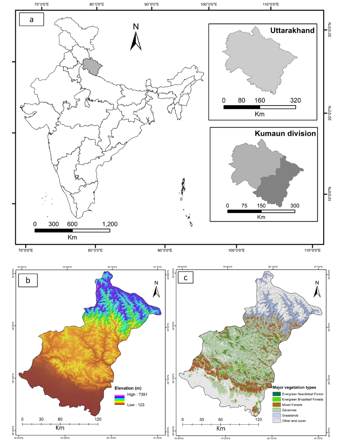
2.1. Study Area

The Kumaon region of the western Himalayas was chosen as the study area, as it offers one of the most diverse biogeographical regions in the Indian Himalayan region. The Kumaun division of Uttarakhand (Figure 1) covers an area of 21,034 km², and is located between latitudes 28°44′ N to 30°49′ N and longitudes 78°45′ E to 81°05′ E with elevations ranging from 200 m to 6000 m above mean sea level (amsl).

The area comes under the humid subtropical climate zone of Koppen’s classification. As per the International Geosphere–Biosphere Programme (IGBP) classification scheme, the dominant vegetation types of Kumaon Himalaya are need-leaf evergreen, broadleaf evergreen, broadleaf deciduous, and mixed forest along with savanna type vegetation and grassland.

The annual mean temperature remains around 13 °C. The hottest month is June (18.3 °C) and the coldest month is January (6.4 °C). The mean annual rainfall is around 1500 mm, where November is the driest (50 mm) and July remains the wettest (500 mm) month. The monthly average relative humidity ranges from 46 percent (in April) to 93 percent (in September), with the yearly average relative humidity coming at 65.9 percent (in August). The species composition and distribution greatly vary along the altitudinal, temperature, and rainfall gradient.

2.2. Datasets

2.2.1. Earth Observation Datasets

The International Geosphere–Biosphere Programme (IGBP) land cover data of coarse (1 km) spatial resolution are used to identify and delineate the forest types of the study area. ALOS PALSER 12.5 m digital elevation data are used to generate an elevation profile and three vegetation indices products of MODIS (LAI, NDVI, EVI) are used to identify and compare the phenological indicator. The MCD12Q1 version 6 data product provides yearly global land cover type data under six different classification schemes. The land cover classes are obtained using yearly metrics as inputs to the random forest classifier, followed by supervised decision tree classification and post-processing of the map results based on Hidden Markov Models, which significantly reduce interannual variability in the product. In the present study land cover class type, one was used, which has 17 classes, including natural vegetation, human-altered, and non-vegetated. This product also includes layers of seasonal cycles, as the beginning of the vegetation’s growth, maturity, and senescence [33]. JAXA provided (ALOS PALSAR) the Digital Elevation Model (DEM) at 12.5 m data that were downloaded from NASA Earth Data’s ASF Data search platform. All the tiles were mosaicked and masked using the boundary of the study area.

2.2.2. Meteorological Datasets

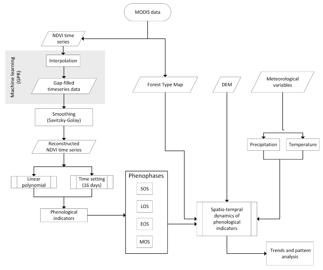
The Integrated Multi-Satellite Retrievals for GPM (IMERG) is used as precipitation data. IMERG is a single algorithm that gives precipitation estimates by merging data from all GPM constellation passive microwave devices. GPM-M data were utilised in this work [34,35]. MODIS11A1 version 6 product data, which offers daily per-pixel land surface temperature and emissivity at 1 km spatial resolution, was used to obtain temperature data. The daily data were acquired utilising the Google Earth Engine (GEE) platform, using an elevation zone-wise shape file. In the R environment, monthly mean values are generated from daily mean temperature data.

2.3. Methodology

In the present investigation, we used DATimeS coupled with Savitzky–Golay (SG), and simplified least square fit convolution to extract the phenophases (SOS and LOS) from MODIS datasets for major vegetation types and used SOS and EOS for the final analysis (Figure 2). Afterwards, a correlation between phenophases and climatic variables (temperature and precipitation) was analyzed.

2.3.1. Retrieval of Vegetation Index and Vegetation Map

The MCD12Q1 version 6 data product was used to extract a vegetation type map, which includes ENF, EBF, MF, savanna, and grassland, which are the major vegetation types present in the study area. The elevation data were masked using individual forest-type layers and further divided into four equal elevation gradient zones (H1, H2, H3, and H4). The MOD13A1 version 6 product derived from daily, atmosphere-corrected, bidirectional surface reflectance, provides two vegetation indices (NDVI, EVI) at 16-day intervals, and 500 m × 500 m pixel size; it provides high sensitivity over dense vegetation with a minimum canopy soil variation. Then, the mean NDVI values for each zone of the study vegetation type were obtained from GEE. LSP and phenometrics were then extracted from smoothed MODIS NDVI time series data from 2001 to 2019. NDVI can be calculated by the NIR and red reflectance [36] as:

$$\mathrm{NDVI}=\frac{\mathrm{NIR}-\mathrm{RED}}{\mathrm{NIR}+\mathrm{RED}}$$

(1)

where:

RED = MODIS band 1 surface reflectance

NIR = MODIS band 2 surface reflectance

2.3.2. Time Series Smoothing and Gap Filling

The MODIS NDVI product data are temporarily composited using a prominence threshold approach to filter out the noisy and erroneous points. A prominence of peak is defined as the shortest vertical distance a signal must travel on either side of the peak before either rising to a level higher than the peak again or reaching an endpoint. This distance may be measured in either direction from the peak. Peaks that do not surpass the present prominence value are thus automatically dismissed as noise.

The GPR approach typically depicts the relationship between input samples and output observations, where the use of an additive Gaussian noise with zero mean function encodes that each location has equal probability. The covariance matrix function is to use a kernel function called K to encode the similarity between each combination of the input sample Xi and Xj. The covariance design is extremely important since it needs to consider the key characteristics of the variables to be modelled. Due to its capacity to correctly estimate smoothly changing functions and also take into account asymmetries in the feature space, the asymmetric square exponential (SE) kernel performs well when vegetation indices are to be retrieved from earth observation data [37,38,39]. The SE kernel is used in the present study and defined as follows:

$$k(x_i,x_j={\sigma }_s^{2}exp\left(-\frac{1}{2}{\displaystyle \sum }_{b=1}^D{\left[\frac{x_i\left(b\right)-x_j\left(b\right)}{{\sigma }_b}\right]}^2\right)$$

(2)

where ${\sigma }_s^2$ denotes the output variance and ${\sigma }_b$ is connected to the dispersion of the training information along the input dimension b in such a manner that the inverse of ${\sigma }_b$ defines the significance of dataset b in the prediction process. Once the noise variance ${\sigma }_n^2$ and the kernel’s free parameters are chosen, the covariance matrix is fully determined. These terms, which are referred to as the hyperparameters of the GPR model, may all be written as $\theta =\left\{{\sigma }_s^2, {\sigma }_{}^2, {\sigma }_n^2\right\}$, where $\sigma$= [${\sigma }_1, \dots , {\sigma }_D$].

$$\log p\left(y|x, f\right)=-\frac{1}{2}{y}^T{\left(\mathsf{{\rm K}}+{\sigma }_n^2{\mathsf{{\rm I}}}_N\right)}^{-1}y-\frac{1}{2}\log \left|\mathsf{{\rm K}}+{\sigma }_n^2{\mathsf{{\rm I}}}_N\right|-\frac{n}{2}\log \pi$$

(3)

where N = number of training samples, K = covariance matrix, and y = training output

The first part in Equation (3) is effectively a data-fit term, the second one is a complexity penalty, and the last term is merely a normalizing constant. The maximisation of the log-likelihood method is used to optimise the hyperparameter in the present study. Training the GPR is the common name for this optimisation process [37,38,40,41].

Following that, the data sets were smoothed using the Savitzky–Golay filter (SG filter), and a time series were reconstructed using the DATimeS tool. The SG filter has a balancing ability to decrease noise while keeping the integrity of the NDVI time series. For NDVI time series smoothing, the general equation for the simplified least-squares convolution is:

$$Y_i{}^{*}=\frac{{{\displaystyle \sum }}_{i=-m}^{i=m}{C}_i{Y}_{j+i}}{N}$$

(4)

where

Y = NDVI value (original),

Y* = NDVI value (resultant),

Ci = coefficient for the i^th NDVI value of the filter (smoothing window), and

N = convoluting number of integers.

Finally, phenological events are obtained from the smoothed time series in order to establish the exact timing of the transition between the various phases of plant development. Only SOS and EOS were taken into consideration in the present study. In this study, to obtain phenological events, the use of a polynomial model with a defined degree and the Savitzky–Golay generalised moving average with the filter coefficient being determined by an unweighted linear least-squares regression [39].

2.3.3. Forest Phenological Variables

The geographical area under investigation is very heterogeneous in nature. The elevational gradient for each vegetation type varies differentially. The threshold-based method is adapted to determine the land surface phenology of the Kumaon forest. According to earlier studies [30,42,43,44,45] the threshold value varies with the forest type and altitudinal gradients and ranges between 0.2 and 0.3. To make a balanced approach across the altitudinal gradient and forest types, a 25% amplitude is used as the threshold to determine SOS and EOS. The SOS NDVI value for the given vegetation type was quantified using the following equation

$${\mathrm{NDVI}}_{start}={\mathrm{NDVI}}_{min}+\left({\mathrm{NDVI}}_{max}-{\mathrm{NDVI}}_{min}\right)\ast 0.25$$

(5)

$${\mathrm{NDVI}}_{end}={\mathrm{NDVI}}_{min}+\left({\mathrm{NDVI}}_{max}-{\mathrm{NDVI}}_{min}\right)\ast 0.25.$$

(6)

The double logistic curve fitting is then used to calculate the SOS and EOS, which can be calculated for any given day using the aforementioned threshold value.

2.3.4. Trend and Correlation Analysis

The trend analysis of the phenological variables is done using the linear regression method. Least square fit algorithm is frequently used to analyse the trend and growth patterns of the vegetation. Further, the correlations between phenometrics and climatic variables are assessed using a linear regression approach. All the statistical analysis is done using the R software package.

The relationship between climatic variables and phenometrics (SOS and EOS) is accomplished using multivariate regression analysis. This step is performed in R statistical software. The equation used in this approach is:

$$Y={\beta }_0+{\beta }_1{X}_1+{\beta }_2{X}_2+\in$$

(7)

where β₀ = model intercept, β₁ β₂ = coefficients, X₁, X₂ = covariates, and ∈ = random error.

3. Results

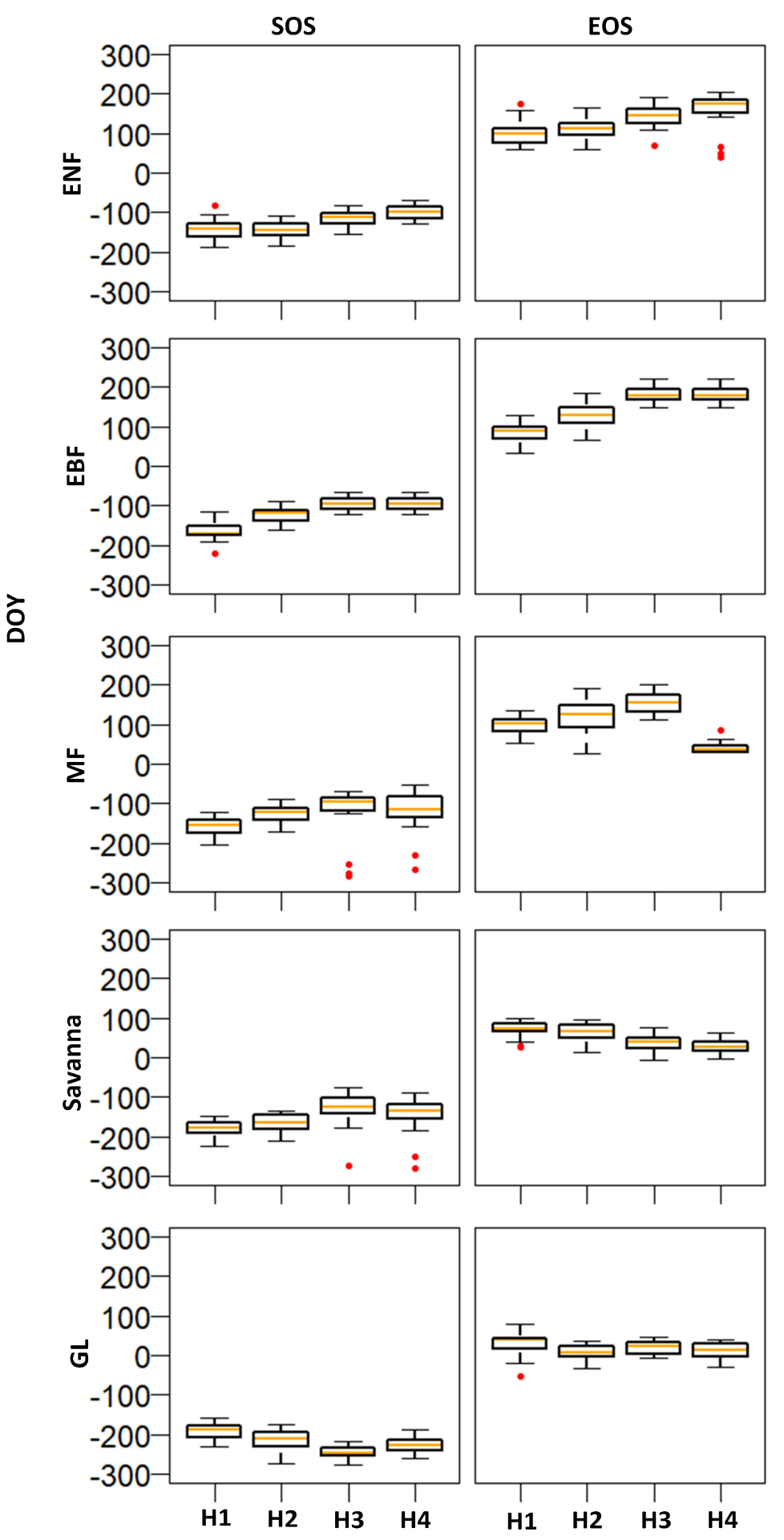
3.1. Spatial Patterns of Phenometrics

Seasonal patterns of plant phenology greatly vary with the vegetation type, latitude, and elevation. The occurrence of SOS varies greatly along the elevation gradient. It even varies considerably within the vegetation type, along the gradient. Both ENF and EBF show a delay (positive) trend in both SOS and EOS. The MF and Savanna show a mixed trend where initially it shows a delayed trend, however, at higher reaches, it starts advancing. GL shows an advancement (negative) trend for both SOS and EOS. Figure 3 exhibits the average SOS and EOS day of the year and its spatial distribution along the elevational gradient. The study shows a consistent pattern in the spatial distribution of phenophases across the vegetation types (Figure 3). The SOS and EOS show a delayed trend for ENF, EBF, and MF. Savanna shows a mixed type of pattern for SOS, where initially it shows a delayed trend up to 2600m and then it becomes reversed and starts advancing (negative) with a rate of 0.7 d/100 m, and the pattern stays similar for the EOS (

Table 1. Spatial distribution of phenometrics trend within vegetation types.

	ENF (1300–2250 m)	EBF (500–2250 m)	MF (800–3000 m)	Savanna (1500–3300 m)	GL (2000–4000 m)
SOS (days/100 m)	1.5	2.4	1.1	1.6 and −0.7	−1.2
EOS (days/100 m)	1.8	2.2	1.9	−1.4	−0.9

). GL shows advancement for SOS, but EOS does not show any significant shift. The highest rate of change in SOS was reported in EBF (2.4 d/100 m) and the lowest rate in the savanna (−0.7 d/100 m). For EOS, the highest rate was in EBF (2.2 d/100 m), but the lowest was in GL (−0.9 d/100 m).

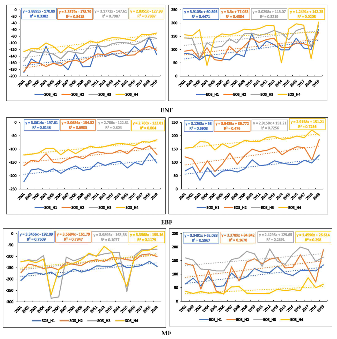
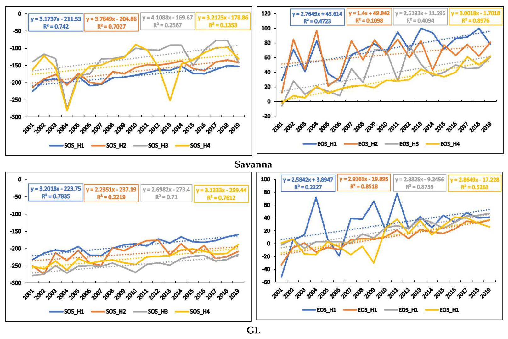
3.2. Interannual Variations in Phenometrics

SOS shows a delay (positive) trend across the vegetation types, the highest rate of change was reported in the upper reaches of grassland (3.3 DY⁻¹) and the lowest in the upper reaches of mixed forest (0.9 DY⁻¹) (Figure 4). Similarly, the EOS shows a varying degree of change across the vegetation types and along the elevation gradient. The lowest rate was reported in ENF (1.2 DY⁻¹) and the highest in GL (2.9 DY⁻¹).

Table 2. Interannual distribution of phenometrics trend in major vegetation types.

	ENF		EBF		MF		Savanna		GL
Elevation Zones	SOS DY−1	EOS DY−1	SOS DY−1	EOS DY−1	SOS DY−1	EOS DY−1	SOS DY−1	EOS DY−1	SOS DY−1	EOS DY−1
H1	2.6	2.9	2.7	2.1	2.0	2.4	2.5	2.8	2.6	2.6
H2	1.8	2.3	1.2	2.9	1.9	2.4	2.5	2.5	3.1	2.9
H3	1.6	2.0	1.2	1.9	1.3	1.9	2.4	2.1	3.7	2.9
H4	1.2	1.2	1.2	1.9	0.9	2.2	2.1	2.0	3.3	2.9

shows the rate of change in interannual variations in SOS and EOS. The overall trend in SOS and EOS is not consistent, but shows a decreasing rate of change along with the increasing elevation (Figure 4).

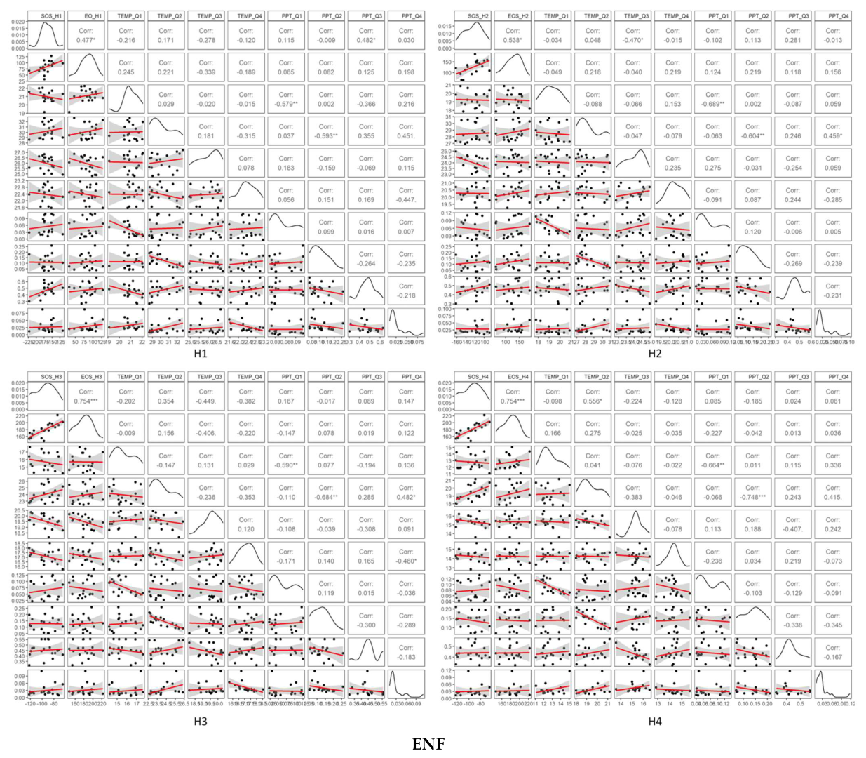
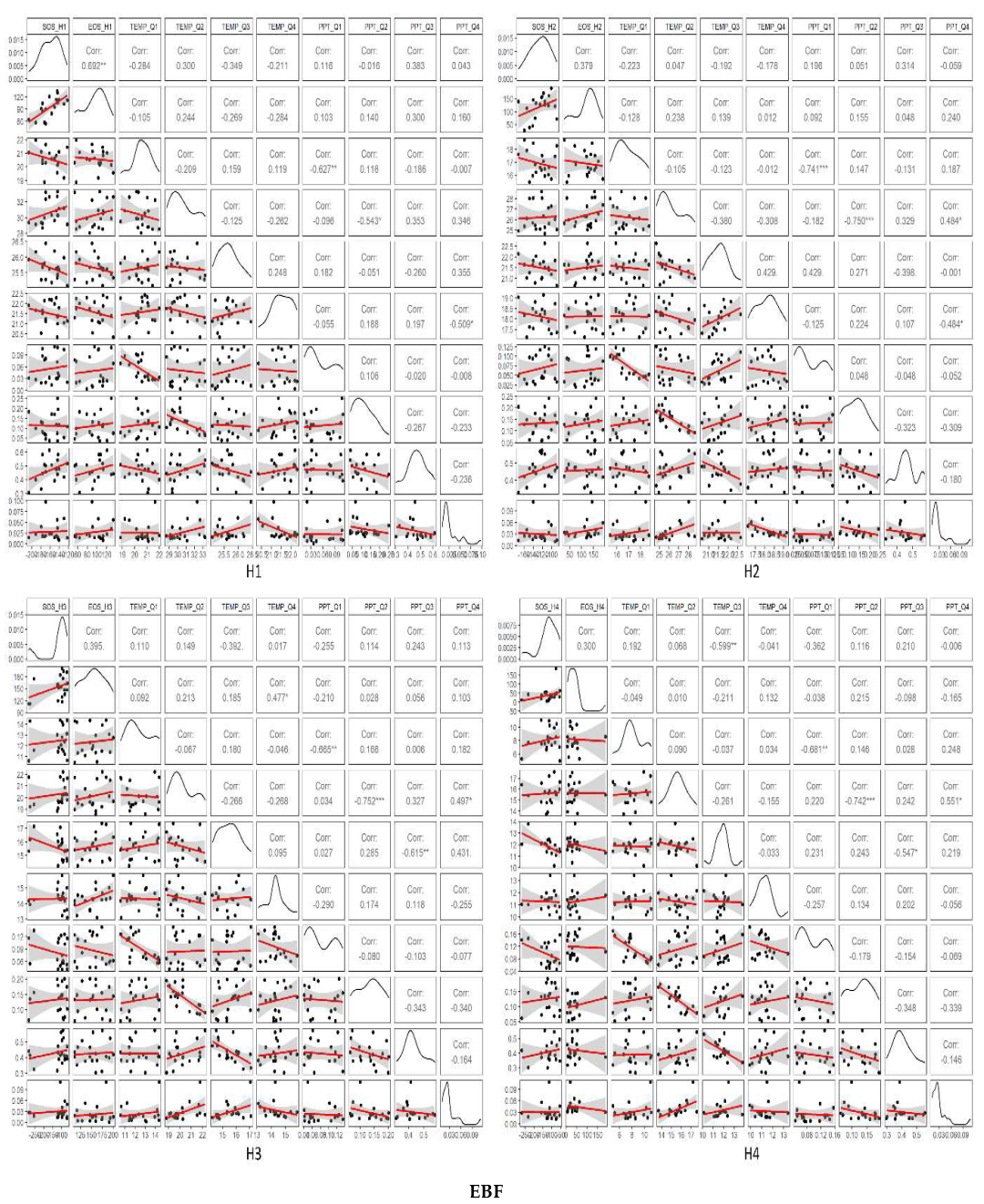
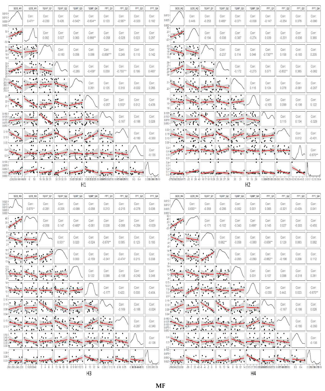
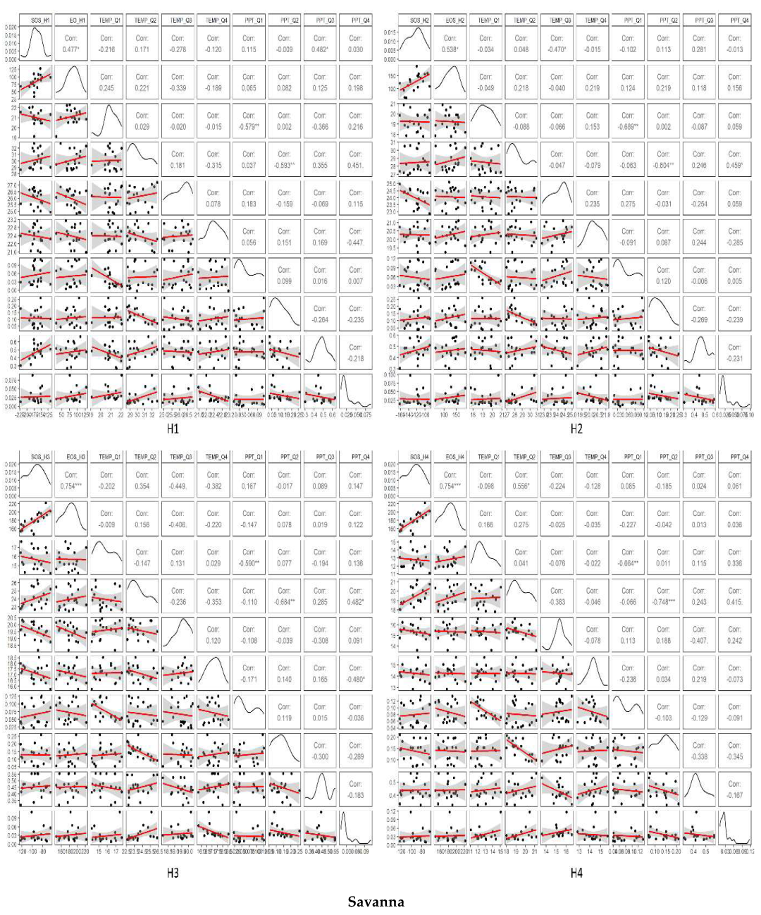
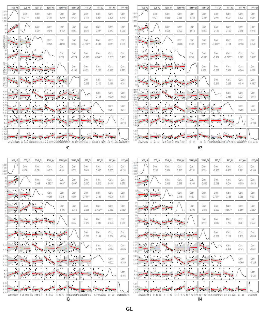
3.3. Temporal Trends of Climatic Variables and the Relationship between Phenometrics and Climatic Variables

In this work, phenometrics were used to analyse the temporal and spatial relationships between LSP and climatic variables. The association between phenological phases and temperature was investigated with the help of partial correlation analysis and multivariate linear regression. This was performed after the precipitation factor was taken into account. In a similar manner, partial correlation analysis was used in order to evaluate the correlations between phenological phases and precipitation after the temperature was adjusted. The correlations between phenometrics and climatic variables were performed using quarterly (Q1, Q2, Q3 and Q4) data of climatic variables. The relationship between temperature and precipitation in the spring (April, May, and June) season, which also coincides with, or is called the preseason period, and winter + autumn (October to March), was assessed using a multivariate linear regression model. The different vegetation types show variable responses towards climatic variables (Figure 5). SOS of most of the vegetation types shows a negative correlation with the spring temperature, while a positive correlation was observed with the precipitation. Temperature shows a moderate to good negative correlation (R > −0.5, p < 0.05) with SOS in preseason months. The SOS of the major vegetation type shows a positive correlation with precipitation. EOS exhibits a significant positive correlation with winter temperature and precipitation and is the most unpredictable at high altitudes and areas with varied species diversity.

4. Discussion

Climate change altered the dynamics of phenological events in areas from tropical to temperate regions. Many plant species show advancement in their spring phases because of climate change. Strong winter warming, on the other hand, could inhibit required winter chilling, perhaps delaying spring phenology. This phenomenon is particularly noticeable in areas where temperatures are rapidly rising and where vegetation is very temperature-responsive.

4.1. Driving Factors for Phenometrics Changes

Spatial and temporal distribution was evaluated across five major vegetation types of Kumaon Himalaya spanning two decades (2001–2019). The mean SOS and EOS time varies across vegetation types and also with latitude and elevation. The onset of vegetative stages showed a shift from June to July at lower reaches to July to August as we moved to the higher elevation, which shows a negative correlation with the general climate change-induced trend. However, in the upper savanna and alpine region, it shows an advanced onset of the season, a positive correlation with the temperature elevation trend. According to recent studies [46,47,48,49], temperature is not the primary governing factor for seasonal behavior along the elevational gradient, but rather the temperature lapse rate due to the elevation gradient, which controls vegetation behavior along the EG in heterogeneous mountainous regions.Our study is also following with these findings and shows a differential behaviour of both SOS and EOS over EG; whereas in MF, Savanna and GL show differential behaviour towards the climatic variable along the EG, even within the vegetation type, because of their large distributional range and topography. As we move upward (lower and middle elevation) it shows a delayed trend in the MF; at higher elevation, it shows a reversal of trend and starts advancing thereafter. Similar results were observed in savanna and GL, they show an advancing trend throughout its EG. These abrupt changes in higher elevation are perhaps influenced by the premature availability of precipitation due to early snowmelt, governed by an increase in soil and ambient temperature. For temporal distribution, all the major vegetation types follow the trends observed in spatial distribution, but the rate of change remains low on the temporal scale in comparison to the spatial scale. This again proves the dominance of lapse rate due to EG across the vegetation types.

4.2. Phenological Changes with Different Gradients

Flowering durations tended to be delayed as elevation increased (−0.07 to 2.2 days/100 m), which is consistent with findings from the Himalayan subalpine environments (0.014 days m1, [46]). The perception that most species show advanced spring phenology was supported by research on phenology changes [47,48,49,50]. However, a significant number (~25%) of species in all of these investigations deviates from this pattern and exhibited trends toward delayed spring phenology. To address this, we divided the elevational gradient into four equal vertical zones to know the change patterns along the altitudinal gradient within the vegetation types. Except for mixed forest and savanna, all the vegetation types show a delayed trend that is in agreement with the findings of various studies in the northern hemisphere [51,52,53]. However, the trends in mixed forest and savanna show the reversal of trends at higher altitudes within the vegetation types. This is because of the weakened temperature effect on higher altitudes. The vertical zones H3 and H4 of mixed forest and savanna, which are overlapped with the grassland show a similar trend as of grassland vegetation. This happens because of the altitude-induced lapse rate, which compensates the climate change-induced warming and reverses the trend at higher altitudes. A few recent studies also observed the trend reversal in grassland and savanna vegetation types at higher altitudes, which supports our findings [52]. These outcomes are not contradictory, but rather show that the change in temperature is generally influenced by the altitudinal gradient in mountainous systems. As the altitude increases the temperature drops constantly and in response, the time to attain accumulated growth temperature for different vegetation types gets altered [53,54,55].

The spring phenology variations indicate that the responses of plants to the warming are not linear and vary by vegetation type and local climatic behaviour [56]. Most temperate and subtropical plants’ spring phases are determined by winter cold and spring heat [57,58,59] Warming in the spring slows spring phenology, whereas warming in the winter delays chilling needs. The surprising tendency of budburst delay in vegetative events is most likely driven by higher temperatures and low precipitation in winter and the hot dry spring season. Temperature (especially the maximum temperature) increases the rate of evapotranspiration during the driest months of the year, eventually increasing loss of soil water content and further reducing the turgor pressures required to expand developing cells [55], potentially delaying the development of leaves. This is perhaps one of the reasons for delayed SOS in addition to winter warming. If there was more water, an optimal thermal condition would reduce plant heat buildup and enhance budburst, and low rainfall and high temperature would delay the budburst.

In the present study, the phenophases show a delayed trend in ENF, EBF, MF, savanna, and GL SOS despite the spring heating, which does not endorse the general trend shown by most of the studies in various parts of the world. The preseason shows a negative correlation with the SOS, which is in agreement with the general trends reported worldwide. The preseason months show a constant increase in temperature and a decline in precipitation in the study period. The dryer conditions created by low precipitation and high temperature further complicate spring phenology’s responses to climate change. In general, the majority of the species vegetative growth and reproductive stages are known to depend on available moisture, whereas blooming and fruiting in plants appear to be related to ambient temperature [57]. The observations in the present study do not confirm the general trend of advancement reported in various studies. Despite the continuous warming of the spring season and phenology-advancing effect [58,59,60,61] of rising temperature in spring, this part of the western Himalayas shows a delayed start of the season. A similar trend was also reported by Delbart et al., 2006, [61]. The increasing temperature in October to march and low precipitation in the same time frame [62], coupled with unfavourable hot and dry conditions in spring, pushed forward the onset of the growing season. The temperature of October, November, February, and March shows a warming trend in the last two decades. The delaying impact could be a result of reduced winter chill, causing plants’ vernalisation requirements to be met later.

Among all the vegetation types, mixed forest shows a differential trend pattern and does not show agreement with the general trend obtained in the study. Remote sensing modelling of phenology works on several trees and site conditions blended together in a pixel, and that leads to no selection of site characteristics and microclimatic conditions of trees or nearby forest areas. The use of a mix of coniferous and broadleaf species proved to affect phenology data, and this is well investigated. The drop in vegetation indices in pixels with a high percentage of coniferous species is expected to be slower near the end of the season in fall than in pixels with pure deciduous broadleaved species, making estimating the date of phenological events more unclear, as was reported in this study [63,64].

Our findings show a delayed trend in EOS date in the Kumaon Himalaya from 2001 to 2019, which is in agreement with the findings of earlier research in the Northern Hemisphere [65], temperate China [66,67,68], Europe [69], and North America [66]. The EOS date shows a delayed trend by a rise in preseason temperature, which was similar to findings from prior research using satellite data and field investigations [67]. This is because of the fact that warming in the summer and autumn boosts photosynthetic activity, slows chlorophyll degradation during leaf senescence in the fall, and hence delays leaf senescence. In all the (ENF, EBF, MF, savanna, and GL) regions, preseason precipitation was likewise inversely linked with the EOS. During the preseason, soil moisture will rapidly increase as precipitation increases, enhancing vegetation photosynthesis via altering vegetation carboxylation. The vegetation will develop more quickly and finish the growing season preschedule [68]. However, in the study area under investigation, precipitation shows a negative trend and as result delays the EOS, which is in confirmation with earlier works.

5. Conclusions

The present study unfolded those disparities in phenology changes caused by climate change in major vegetation types of Himalayan Forest ecosystems. We emphasised how different major vegetation types respond to changes in climatic variables at spatial and temporal scales. This study highlighted the necessity for rigorous research into plant phenology in understudied Himalayan forests. Warmer ecosystems control phenology differently than better-studied temperate systems; prediction of spring phenology changes in warmer ecosystems that overlook late summer and early fall temperatures might be misleading. Subtropical plants bloom all year and respond to temperature changes differently than temperate plants. However, subtropical and temperate forests, respond to climate change differently. This study tried to bring some new insight into the field of plant phenology, as there were not many area-specific or vegetation-specific studies on Himalayan ecosystems to study the climate-induced changes along the elevational gradient. For improving our fundamental knowledge of forest ecology and for influencing management and policy choices related to climate and conservation, it is crucial to understand the differences in the mechanisms that govern phenology in forest ecosystems. This research is therefore required to better comprehend climate-driven phenological shifts and forecast future changes in tropical and subtropical environments, which are essential to the environment, ecosystems, and conservation. Awareness of the consequences of climate change on vegetation phenology and ecosystem processes will require an understanding of these changes. The results of this study indicate the importance of the elevation gradient and its relationship with climatic variables among and within the vegetation types. Further research with robust ground truth data and long-term meteorological data from the ground station using better spatial resolution data sets would be helpful in understanding the variations in phenological patterns and complex interaction between climatic variables, elevation, and phenophases.

References

1. Wang, X.; Gao, Q.; Wang, C.; Yu, M. Spatiotemporal patterns of vegetation phenology change and relationships with climate in the two transects of East China. Glob. Ecol. Conserv. 2017, 10, 206–219. [Google Scholar] [CrossRef]
2. Wang, X.; Xiao, J.; Li, X.; Cheng, G.; Ma, M.; Che, T.; Dai, L.; Wang, S.; Wu, J. No Consistent Evidence for Advancing or Delaying Trends in Spring Phenology on the Tibetan Plateau. J. Geophys. Res. Biogeosci. 2017, 122, 3288–3305. [Google Scholar] [CrossRef] [Green Version]
3. Richardson, A.D.; Hollinger, D.Y.; Dail, D.B.; Lee, J.T.; Munger, J.W.; O’keefe, J. Influence of spring phenology on seasonal and annual carbon balance in two contrasting New England forests. Tree Physiol. 2009, 29, 321–331. [Google Scholar] [CrossRef]
4. Piao, S.; Cui, M.; Chen, A.; Wang, X.; Ciais, P.; Liu, J.; Tang, Y. Altitude and temperature dependence of change in the spring vegetation green-up date from 1982 to 2006 in the Qinghai-Xizang Plateau. Agric. For. Meteorol. 2011, 151, 1599–1608. [Google Scholar] [CrossRef]
5. Cong, N.; Wang, T.; Nan, H.; Ma, Y.; Wang, X.; Myneni, R.B.; Piao, S. Changes in satellite-derived spring vegetation green-up date and its linkage to climate in China from 1982 to 2010: A multimethod analysis. Glob. Chang. Biol. 2013, 19, 881–891. [Google Scholar] [CrossRef]
6. Shen, M.; Piao, S.; Cong, N.; Zhang, G.; Jassens, I.A. Precipitation impacts on vegetation spring phenology on the Tibetan Plateau. Glob. Chang. Biol. 2015, 21, 3647–3656. [Google Scholar] [CrossRef] [Green Version]
7. Peng, D.; Wu, C.; Li, C.; Zhang, X.; Liu, Z.; Ye, H.; Luo, S.; Liu, X.; Hu, Y.; Fang, B. Spring green-up phenology products derived from MODIS NDVI and EVI: Intercomparison, interpretation and validation using National Phenology Network and AmeriFlux observations. Ecol. Indic. 2017, 77, 323–336. [Google Scholar] [CrossRef]
8. Wang, X.; Zhou, Y.; Wen, R.; Zhou, C.; Xu, L.; Xi, X. Mapping spatiotemporal changes in vegetation growth peak and the response to climate and spring phenology over northeast China. Remote Sens. 2020, 12, 3977. [Google Scholar] [CrossRef]
9. Liu, Q.; Fu, Y.H.; Zeng, Z.; Huang, M.; Li, X.; Piao, S. Temperature, precipitation, and insolation effects on autumn vegetation phenology in temperate China. Glob. Chang. Biol. 2016, 22, 644–655. [Google Scholar] [CrossRef]
10. Ni, W.; Sun, G.; Pang, Y.; Zhang, Z.; Liu, J.; Yang, A.; Wang, Y.; Zhang, D. Mapping Three-Dimensional Structures of Forest Canopy Using UAV Stereo Imagery: Evaluating Impacts of Forward Overlaps and Image Resolutions with LiDAR Data as Reference. IEEE J. Sel. Top. Appl. Earth Obs. Remote Sens. 2018, 11, 3578–3589. [Google Scholar] [CrossRef]
11. Hmimina, G.; Dufrêne, E.; Pontailler, J.Y.; Delpierre, N.; Aubinet, M.; Caquet, B.; de Grandcourt, A.; Burban, B.; Flechard, C.; Granier, A.; et al. Evaluation of the potential of MODIS satellite data to predict vegetation phenology in different biomes: An investigation using ground-based NDVI measurements. Remote Sens. Environ. 2013, 132, 145–158. [Google Scholar] [CrossRef]
12. Bórnez, K.; Descals, A.; Verger, A.; Peñuelas, J. Land surface phenology from VEGETATION and PROBA-V data. Assessment over deciduous forests. Int. J. Appl. Earth Obs. Geoinf. 2020, 84, 101974. [Google Scholar] [CrossRef]
13. Baldocchi, D.D.; Black, T.A.; Curtis, P.S.; Falge, E.; Fuentes, J.D.; Granier, A.; Gu, L.; Knohl, A.; Pilegaard, K.; Schmid, H.P.; et al. Predicting the onset of net carbon uptake by deciduous forests with soil temperature and climate data: A synthesis of FLUXNET data. Int. J. Biometeorol. 2005, 49, 377–387. [Google Scholar] [CrossRef]
14. Jönsson, P.; Eklundh, L. TIMESAT—A program for analyzing time-series of satellite sensor data. Comput. Geosci. 2004, 30, 833–845. [Google Scholar] [CrossRef] [Green Version]
15. Sobrino, J.A.; Julien, Y. Global trends in NDVI-derived parameters obtained from GIMMS data. Int. J. Remote Sens. 2011, 32, 4267–4279. [Google Scholar] [CrossRef]
16. Richardson, A.D.; Keenan, T.F.; Migliavacca, M.; Ryu, Y.; Sonnentag, O.; Toomey, M. Climate change, phenology, and phenological control of vegetation feedbacks to the climate system. Agric. For. Meteorol. 2013, 169, 156–173. [Google Scholar] [CrossRef]
17. Misra, G.; Asam, S.; Menzel, A. Ground and satellite phenology in alpine forests are becoming more heterogeneous across higher elevations with warming. Agric. For. Meteorol. 2021, 303, 108383. [Google Scholar] [CrossRef]
18. Broich, M.; Huete, A.; Paget, M.; Ma, X.; Tulbure, M.; Coupe, N.R.; Evans, B.; Beringer, J.; Devadas, R.; Davies, K.; et al. A spatially explicit land surface phenology data product for science, monitoring and natural resources management applications. Environ. Model. Softw. 2015, 64, 191–204. [Google Scholar] [CrossRef]
19. Julien, Y.; Sobrino, J.A. Global land surface phenology trends from GIMMS database. Int. J. Remote Sens. 2009, 30, 3495–3513. [Google Scholar] [CrossRef] [Green Version]
20. Zeng, L.; Wardlow, B.D.; Xiang, D.; Hu, S.; Li, D. A review of vegetation phenological metrics extraction using time-series, multispectral satellite data. Remote Sens. Environ. 2020, 237, 11511. [Google Scholar] [CrossRef]
21. Du, J.; Li, K.; He, Z.; Chen, L.; Lin, P.; Zhu, X. Daily minimum temperature and precipitation control on spring phenology in arid-mountain ecosystems in China. Int. J. Climatol. 2020, 40, 2568–2579. [Google Scholar] [CrossRef]
22. Zhang, X.; Zhai, P.; Huang, J.; Zhao, X.; Dong, K. Responses of ecosystem water use efficiency to spring snow and summer water addition with or without nitrogen addition in a temperate steppe. PLoS ONE 2018, 13, e0194198. [Google Scholar] [CrossRef] [Green Version]
23. Zhang, X.; Friedl, M.A.; Schaaf, C.B.; Strahler, A.H. Climate controls on vegetation phenological patterns in northern mid- and high latitudes inferred from MODIS data. Glob. Chang. Biol. 2004, 10, 1133–1145. [Google Scholar] [CrossRef]
24. Wang, Y.; Li, G.; Ding, J.; Guo, Z.; Tang, S.; Liu, R.; Chen, J. A combined GLAS and MODIS estimation of the global distribution of mean forest canopy height. Remote Sens. Environ. 2016, 174, 24–43. [Google Scholar] [CrossRef]
25. Araya, S.; Ostendorf, B.; Lyle, G.; Lewis, M. CropPhenology: An R package for extracting crop phenology from time series remotely sensed vegetation index imagery. Ecol. Inform. 2018, 46, 45–56. [Google Scholar] [CrossRef]
26. Hill, M.J.; Donald, G.E. Estimating spatio-temporal patterns of agricultural productivity in fragmented landscapes using AVHRR NDVI time series. Remote Sens. Environ. 2003, 84, 367–384. [Google Scholar] [CrossRef]
27. Lloyd, D. A phenological classification of terrestrial vegetation cover using shortwave vegetation index imagery. Int. J. Remote Sens. 1990, 11, 2269–2279. [Google Scholar] [CrossRef]
28. White, M.A.; Nemani, R.R. Real-time monitoring and short-term forecasting of land surface phenology. Remote Sens. Environ. 2006, 104, 43–49. [Google Scholar] [CrossRef]
29. Huang, X.; Liu, J.; Zhu, W.; Atzberger, C.; Liu, Q. The optimal threshold and vegetation index time series for retrieving crop phenology based on a modified dynamic threshold method. Remote Sens. 2019, 11, 2725. [Google Scholar] [CrossRef] [Green Version]
30. Friedl, M. MODIS Collection 5 global land cover: Algorithm refinements and characterization of new datasets. Remote Sens. Environ. 2010, 114, 168–182. [Google Scholar] [CrossRef]
31. Sharifi, E.; Steinacker, R.; Saghafian, B. Assessment of GPM-IMERG and other precipitation products against gauge data under different topographic and climatic conditions in Iran: Preliminary results. Remote Sens. 2016, 8, 135. [Google Scholar] [CrossRef] [Green Version]
32. Sun, S.; Song, Z.; Wu, X.; Wang, T.; Wu, Y.; Du, W.; Che, T.; Huang, C.; Zhang, X.; Ping, B.; et al. Spatio-temporal variations in water use efficiency and its drivers in China over the last three decades. Ecol. Indic. 2018, 94, 292–304. [Google Scholar] [CrossRef]
33. Huete, A.; Justice, C.; Liu, H. Development of vegetation and soil indices for MODIS-EOS. Remote Sens. Environ. 1994, 49, 224–234. [Google Scholar] [CrossRef]
34. Noumonvi, K.D.; Oblišar, G.; Žust, A.; Vilhar, U. Empirical approach for modelling tree phenology in mixed forests using remote sensing. Remote Sens. 2021, 13, 3015. [Google Scholar] [CrossRef]
35. Belda, S.; Pipia, L.; Morcillo-Pallarés, P.; Verrelst, J. Optimizing Gaussian Process Regression for Image Time Series Gap-Filling and Crop Monitoring. Agronomy 2020, 10, 618. [Google Scholar] [CrossRef]
36. Belda, S.; Pipia, L.; Morcillo-Pallarés, P.; Rivera-Caicedo, J.P.; Amin, E.; De Grave, C.; Verrelst, J. DATimeS: A machine learning time series GUI toolbox for gap-filling and vegetation phenology trends detection. Environ. Model. Softw. 2020, 127, 104666. [Google Scholar] [CrossRef]
37. Borges, E.F.; Sano, E.E.; Medrado, E. Radiometric quality and performance of TIMESAT for smoothing moderate resolution imaging spectroradiometer enhanced vegetation index time series from western Bahia State, Brazil. J. Appl. Remote Sens. 2014, 8, 083580. [Google Scholar] [CrossRef]
38. García-Haro, F.J.; Campos-Taberner, M.; Muñoz-Marí, J.; Laparra, V.; Camacho, F.; Sánchez-Zapero, J.; Camps-Valls, G. Derivation of global vegetation biophysical parameters from EUMETSAT Polar System. ISPRS J. Photogramm. Remote Sens. 2018, 139, 57–74. [Google Scholar] [CrossRef]
39. Yu, X.; Zhuang, D.; Chen, H.; Hou, X. Forest classification based on MODIS time series and vegetation phenology. Int. Geosci. Remote Sens. Symp. 2004, 4, 2369–2372. [Google Scholar] [CrossRef]
40. Shrestha, U.B.; Gautam, S.; Bawa, K.S. Widespread climate change in the Himalayas and associated changes in local ecosystems. PLoS ONE 2012, 7, e36741. [Google Scholar] [CrossRef]
41. Jönsson, P.; Eklundh, L. Seasonality extraction by function fitting to time-series of satellite sensor data. IEEE Trans. Geosci. Remote Sens. 2002, 40, 1824–1832. [Google Scholar] [CrossRef]
42. Myneni, R.B.; Keeling, C.D.; Tucker, C.J.; Asrar, G.; Nemani, R.R. Increased plant growth in the northern high latitudes from 1981 to 1991. Nature 1997, 386, 698–702. [Google Scholar] [CrossRef]
43. Li, H.; Jiang, J.; Chen, B.; Li, Y.; Xu, Y.; Shen, W. Pattern of NDVI-based vegetation greening along an altitudinal gradient in the eastern Himalayas and its response to global warming. Environ. Monit. Assess. 2016, 188, 186. [Google Scholar] [CrossRef]
44. Wang, X.; Piao, S.; Ciais, P.; Li, J.; Friedlingstein, P.; Koven, C.; Chen, A. Spring temperature change and its implication in the change of vegetation growth in North America from 1982 to 2006. Proc. Natl. Acad. Sci. USA 2011, 108, 1240–1245. [Google Scholar] [CrossRef] [Green Version]
45. Piao, S. Growing season extension and its impact on terrestrial carbon cycle in the Northern Hemisphere over the past 2 decades. Glob. Biogeochem. Cycles 2007, 21, 1–11. [Google Scholar] [CrossRef]
46. Zeng, Z. Regional air pollution brightening reverses the greenhouse gases induced warming-elevation relationship. Geophys. Res. Lett. 2015, 42, 4563–4572. [Google Scholar] [CrossRef]
47. Hart, R.; Salick, J.; Ranjitkar, S.; Xu, J. Herbarium specimens show contrasting phenological responses to Himalayan climate. Proc. Natl. Acad. Sci. USA 2014, 111, 10615–10619. [Google Scholar] [CrossRef] [Green Version]
48. Menzel, A.; Sparks, T.H.; Estrella, N.; Koch, E.; Aaasa, A.; Ahas, R.; Alm-Kübler, K.; Bissolli, P.; Braslavská, O.; Briede, A.; et al. European phenological response to climate change matches the warming pattern. Glob. Chang. Biol. 2006, 12, 1969–1976. [Google Scholar] [CrossRef]
49. Parmesan, C. Influences of species, latitudes and methodologies on estimates of phenological response to global warming. Glob. Chang. Biol. 2007, 13, 1860–1872. [Google Scholar] [CrossRef]
50. Fitter, A.H.; Fitter, R.S.R. Rapid changes in flowering time in British plants. Science 2002, 296, 1689–1691. [Google Scholar] [CrossRef]
51. Pellerin, M.; Delestrade, A.; Mathieu, G.; Rigault, O.; Yoccoz, N.G. Spring tree phenology in the Alps: Effects of air temperature, altitude and local topography. Eur. J. For. Res. 2012, 131, 1957–1965. [Google Scholar] [CrossRef]
52. Shen, M.; Zhang, G.; Cong, N.; Wang, S.; Kong, W.; Piao, S. Increasing altitudinal gradient of spring vegetation phenology during the last decade on the Qinghai-Tibetan Plateau. Agric. For. Meteorol. 2014, 189, 71–80. [Google Scholar] [CrossRef]
53. Du, J.; He, Z.; Piatek, K.B.; Chen, L.; Lin, P.; Zhu, X. Interacting effects of temperature and precipitation on climatic sensitivity of spring vegetation green-up in arid mountains of China. Agric. For. Meteorol. 2019, 269, 71–77. [Google Scholar] [CrossRef]
54. Peng, H.; Xia, H.; Chen, H.; Zhi, P.; Xu, Z. Spatial variation characteristics of vegetation phenology and its influencing factors in the subtropical monsoon climate region of southern China. PLoS ONE 2021, 16, e0250825. [Google Scholar] [CrossRef]
55. Suonan, J.; Classen, A.T.; Sanders, N.J.; He, J.-S. Plant phenological sensitivity to climate change on the Tibetan Plateau and relative to other areas of the world. Ecosphere 2019, 10, e02543. [Google Scholar] [CrossRef]
56. Linkosalo, T.; Lappalainen, H.K.; Hari, P. A comparison of phenological models of leaf bud burst and flowering of boreal trees using independent observations. Tree Physiol. 2008, 28, 1873–1882. [Google Scholar] [CrossRef] [Green Version]
57. Luedeling, E.; Gebauer, J.; Buerkert, A. Climate change effects on winter chill for tree crops with chilling requirements on the Arabian Peninsula. Clim. Chang. 2009, 96, 219–237. [Google Scholar] [CrossRef] [Green Version]
58. Green, P.B.; Cummins, W.R. Growth Rate and Turgor Pressure: Auxin Effect Studies with an Automated Apparatus for Single Coleoptiles 1. Plant Physiol. 1974, 54, 863. [Google Scholar] [CrossRef] [Green Version]
59. Bisht, V.K.; Kuniyal, C.P.; Bhandari, A.K.; Nautiyal, B.P.; Prasad, P. Phenology of plants in relation to ambient environment in a subalpine forest of Uttarakhand, western Himalaya. Physiol. Mol. Biol. Plants 2014, 20, 399–403. [Google Scholar] [CrossRef] [Green Version]
60. Chmielewski, F.M.; Rotzer, T. Response of tree phenology to climate change across Europe. Agric. For. Meteorol. 2001, 108, 101–112. [Google Scholar] [CrossRef]
61. Delbart, N.; Le Toan, T.; Kergoat, L.; Fedotova, V. Remote sensing of spring phenology in boreal regions: A free of snow-effect method using NOAA-AVHRR and SPOT-VGT data (1982-2004). Remote Sens. Environ. 2006, 101, 52–62. [Google Scholar] [CrossRef]
62. Yu, H.; Luedeling, E.; Xu, J. Winter and spring warming result in delayed spring phenology on the Tibetan Plateau. Proc. Natl. Acad. Sci. USA 2010, 107, 22151–22156. [Google Scholar] [CrossRef] [Green Version]
63. Henebry, G.M.; de Beurs, K.M. Remote Sensing of Land Surface Phenology: A Prospectus. In Phenology: An Integrative Environmental Science; Schwartz, M.D., Ed.; Springer Netherlands: Dordrecht, The Netherlands, 2013; pp. 385–411. ISBN 978-94-007-6925-0. [Google Scholar]
64. White, K.; Pontius, J.; Schaberg, P. Remote sensing of spring phenology in northeastern forests: A comparison of methods, field metrics and sources of uncertainty. Remote Sens. Environ. 2014, 148, 97–107. [Google Scholar] [CrossRef]
65. Liu, Q.; Fu, Y.H.; Zhu, Z.; Liu, Y.; Liu, Z.; Huang, M.; Janssens, I.A.; Piao, S. Delayed autumn phenology in the Northern Hemisphere is related to change in both climate and spring phenology. Glob. Chang. Biol. 2016, 22, 3702–3711. [Google Scholar] [CrossRef]
66. Zhao, J.; Wang, Y.; Zhang, Z.; Zhang, H.; Guo, X.; Yu, S.; Du, W.; Huang, F. The variations of land surface phenology in Northeast China and its responses to climate change from 1982 to 2013. Remote Sens. 2016, 8, 400. [Google Scholar] [CrossRef] [Green Version]
67. Tang, H.; Li, Z.; Zhu, Z.; Chen, B.; Zhang, B.; Xin, X. Variability and climate change trend in vegetation phenology of recent decades in the Greater Khingan Mountain area, Northeastern China. Remote Sens. 2015, 7, 11914–11932. [Google Scholar] [CrossRef] [Green Version]
68. Yang, Y.; Guan, H.; Shen, M.; Liang, W.; Jiang, L. Changes in autumn vegetation dormancy onset date and the climate controls across temperate ecosystems in China from 1982 to 2010. Glob. Chang. Biol. 2015, 21, 652–665. [Google Scholar] [CrossRef]
69. Stöckli, R.; Vidale, P.L. European plant phenology and climate as seen in a 20-year AVHRR land-surface parameter dataset. Int. J. Remote Sens. 2004, 25, 3303–3330. [Google Scholar] [CrossRef]
Figure 1. (a). Study area location, (b) elevation gradient, and (c) major vegetation type map.
Forests 13 01973 g001
Figure 2. Flowchart of functions used in the present study.
Forests 13 01973 g002
Figure 3. Phenometrics distribution along the elevation gradient across the vegetation types. The positive and negative values indicate starting in the current year and ending in the next year, respectively. The x-axis labels are the subzones divided along the altitudinal gradient of the vegetation types.
Forests 13 01973 g003
Figure 4. Interannual change trend of phenometrics (SOS and EOS) for years from 2001 to 2019 with different vegetation types.
Forests 13 01973 g004aForests 13 01973 g004b
Figure 5. Relationship between phenometrics (SOS and EOS) and climatic variables (temperature and precipitation). The upper triangle consists of correlation value (R2) with significant (p value), and diagonal axis shows the density and lower triangle scatter plot with regression fit line. Here H1, H2, H3, and, H4 are the subzones divided along the altitudinal gradient of the vegetation types. The level of significance is depicted by asterisk (* p ≤ 0.05, ** p ≤ 0.01, and *** p ≤ 0.001).
Forests 13 01973 g005aForests 13 01973 g005bForests 13 01973 g005cForests 13 01973 g005dForests 13 01973 g005e