Assessing the Dependencies of Scots Pine (Pinus sylvestris L.) Structural Characteristics and Internal Wood Property Variation

Abstract

Wood density is well known to vary between tree species as well as within and between trees of a certain species depending on the growing environment causing uncertainties in forest biomass and carbon storage estimation. This has created a need to develop novel methodologies to obtain wood density information over multiple tree communities, landscapes, and ecoregions. Therefore, the aim of this study was to evaluate the dependencies between structural characteristics of Scots pine (Pinus sylvestris L.) tree communities and internal wood property (i.e., mean wood density and ring width) variations at breast height. Terrestrial laser scanning was used to derive the structural characteristics of even-aged Scots pine dominated forests with varying silvicultural treatments. Pearson’s correlations and linear mixed effect models were used to evaluate the interactions. The results show that varying silvicultural treatments did not have a statistically significant effect on the mean wood density. A notably stronger effect was observed between the structural characteristics and the mean ring width within varying treatments. It can be concluded that single time terrestrial laser scanning is capable of capturing the variability of structural characteristics and their interactions with mean ring width within different silvicultural treatments but not the variation of mean wood density.

1. Introduction

Wood density of a tree species is widely expressed as a value on basic wood density -tables existing in scientific literature where it is determined as an oven-dry mass per green volume (kg m⁻³) even though it is rather well known to have major variation within and between trees [1]. Wood density is predominantly determined by the cell wall thickness and lumen size that are known to vary annually depending on the early- and latewood ratio and to change as the tree ages and grows in size. Especially, the amount of thick-walled latewood tracheids and ring width have shown the highest influence on wood density [1,2]. In addition, the transition from pith towards bark (i.e., between juvenile and mature wood) has shown to be a major source of variation of wood density [1].

Wood density is also known to be a site-specific parameter as a result of each individual tree adapting to its growing environment. Different tree species typically have their unique growth rhythm depending on their need for light (i.e., pioneer or shade tolerant trees), and the plasticity of their crowns [3], but competition from water, nutrients and space causes individual trees to deviate from it and allocate growth differently within a forest [4]. Primary growth of a tree occurs at the apex (tips) of stem, branches and roots increasing their length. Thus, by increasing height and crown area for photosynthesis, trees try to improve their status regarding competition within a forest stand. Secondary growth occurs in cambium or in lateral meristems producing secondary xylem and causing diameter growth of a stem, branches, and roots. Secondary xylem (or sapwood) is responsible for the flow of water between functional parts of a tree, as well as structural support. The properties of the secondary xylem (i.e., wood properties) adapt to the increasing tree size and height, in other words to maintain the transportation of water and carry the increasing weight of the crown. Secondary growth is also strongly affected by competition and especially the spatial distribution of trees (i.e., growth space) causing variation in diameter growth allocation and wood properties in different parts of a stem.

Silviculture is a way to influence the spatial distribution of trees within a forest creating space and increase growth, as well as to select tree individuals with the most desired properties. However, the way trees adapt to changes caused by human interventions (i.e., silvicultural operations) within a forest can vary and create considerably different outcomes of external characteristics of trees even between stands with similar stand establishment procedures. Silvicultural activities may aim to produce high quantities of high quality sawn timber to provide the maximum economical value for the owner and the industry. However, many previous studies suggest that the increased growth has caused reduction in wood quality through affecting several influential wood properties such as wood density and knottiness [5,6,7,8].

Previous research has also shown that wood density can decrease due to acceleration in earlywood formation in relation to latewood caused by increased tree radial growth [9,10]. However, the reduction in wood density through accelerated growth after silvicultural activities is not unambiguous. For example, Mäkinen and Hynynen [11] found only a rather low reduction in wood density after intensive thinning that supports the suggestion by Jaakkola et al. [12] that more intensive thinning than is conventional is required to substantially decrease wood density. Similar findings were reported by Peltola et al. [13] where less than a 2% decrease on average in wood density was observed after heavy thinning. Due to the differences in growth allocation and wood formation within and between years, wood density exhibits variable trends with respect to tree species, age and geographical region [14,15,16,17,18]. For example, Piispanen et al. [18] showed that change in competition status of a tree (suppressed or dominant) in uneven-aged forests resulted in fluctuations of wood density from stem pith towards bark, due to its effects on the maturation of wood properties.

At the moment, the only viable way to measure wood density requires destructive sampling or boring samples from standing trees and laboratory measurements. In addition, the lack of methods to characterize the external architecture of trees and their competition status within a forest has been limiting our understanding on tree growth allocation and wood formation. Therefore, previous research has mainly focused on linking growth characteristics (e.g., diameter increment) to wood density variation [11,13,19,20] and rarely utilized detailed size or shape characteristics, or competition status of a tree. The methodological development within the last two decades using terrestrial laser scanning (TLS) acquired three-dimensional data to describe the external architecture of an individual tree [21,22,23,24,25,26] or tree communities [27,28,29,30,31,32] has reached the point where characterization of tree crown and branch properties [33,34,35,36,37] in addition to the stem taper measurements [21,25,38,39,40] are possible. However, Pyörälä et al. [35,36] concluded that comprehensive branch distribution of a tree remains challenging to capture due to the occlusion effect and increasing distance to the scanner at higher parts of the living crown, thus, reducing the quality of a TLS point cloud. The results in Pyörälä et al. [36] demonstrated that the branch detection accuracy decreases dramatically above living crown base height.

In addition to the characterization of external structural attributes, the benefit of TLS data is its capability to capture details of the competition status and location of individual trees (i.e., spatial distribution) within a forest. However, it is known that forest structure and data acquisition strategy has a significant effect on the comprehensiveness of the point cloud [29,32] and thus affect the outcome of forest characterization. In Liang et al. [29], 18 different state-of-the-art algorithms in detecting and characterizing trees were evaluated using 24 structurally varying sample plots. In addition, Yrttimaa et al. [32] evaluated a newly developed algorithm with 91 sample plots within the same study site as Liang et al. [29]. The results in both studies concluded that the complexity of the forest correlated negatively with tree detection accuracy. In addition, Wilkes et al. [31] suggested that the most uniform point distribution with sufficient point cloud quality could be achieved with a systematic grid (e.g., 10 × 10 m) of scanning locations. Recent results in Yrttimaa et al. [41] suggested that high accuracy in characterizing forest structure can be achieved in managed forest stands due to favorable conditions for TLS data acquisition (i.e., ground vegetation removal). They concluded that stem density (number per hectare) and the proportion of suppressed trees were the main factors affecting outcome.

Recently, the interest in wood density information has increased for example due to the uncertainty it is causing to forest biomass and carbon storage estimation. In addition, wood density and ring width are also important determinants of timber quality creating a need to obtain wood density information over multiple tree communities, landscapes and ecoregions. However, there has been a lack of technologies and methods capable of characterizing tree architecture and the structure of the surrounding forest that could be linked to the wood density variation. Previous studies have shown that tree growth and wood formation processes determine the external tree architecture and variation in tree growth process causes variation to wood density. Additionally, with TLS, it is possible to characterize the structure of tree communities. Therefore, the aim of this study was to evaluate the dependencies between TLS-derived structural characteristics and internal wood property (i.e., mean wood density and ring width) variation at breast height (1.3 m) of Scots pine trees. The main research questions (RQ) were: (RQ1) How do varying silvicultural (i.e., thinning) treatments affect wood property variation of trees and tree communities (RQ1)? What are the most influential characteristics explaining internal wood property variation of the trees and how much of the internal wood property variation can be explained with these characteristics (RQ2)? To explore the research questions the following hypotheses were set: Intensive silvicultural treatment will cause lower and more variable wood density values due to increased tree growth (H1); Increased growth, characterized by indicators describing the structural characteristics of a tree and tree community derived from TLS point clouds, could be used to explain most of the internal wood property variation within and between tree communities (H2).

2. Materials and Methods

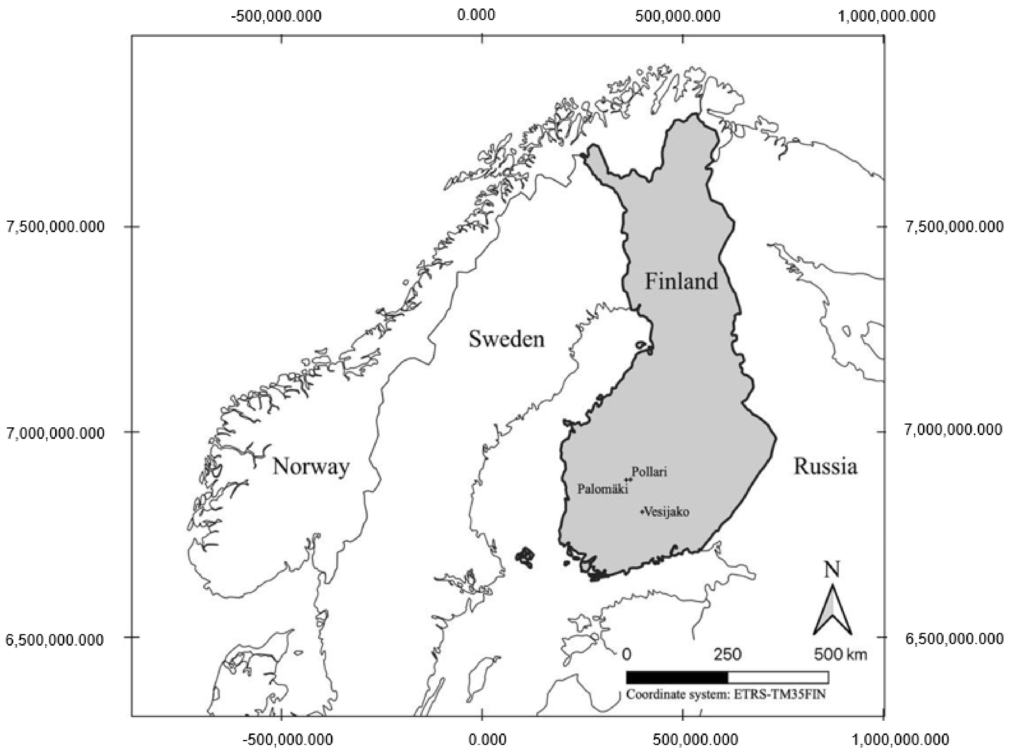
2.1. Study Site

The three study sites were established in southern Finland in 2005 (Palomäki (62°3.6′ N 24°19.9′ E)) and in 2006 (Pollari (62°4.4′ N 24°30.1′ E) and Vesijako (61°21.8′ N 25°6.3′ E)) (Figure 1) and maintained by Natural Resources Institute Finland (Luke). Study sites consist of even-aged (approximately 50 years) Scots pine (Pinus sylvestris L.)-dominated forests. Each study site is characterized as mesic heath forest (i.e., Myrtillus forest site type according to a theory by A. K. Cajander [42]). At the time of establishment, nine rectangular sample plots for each study site (i.e., 27 sample plots in total) with a size varying from 1000 m² to 1200 m² were placed. The experimental design included three thinning types with two different levels of thinning intensity (i.e., moderate and intensive) resulting in six different treatments in total. The three different thinning types were, namely: thinning from below, thinning from above, and systematic thinning. In thinning from below, suppressed and co-dominant trees were removed, whereas in thinning from above mostly dominant trees were removed with the limitation of maintaining regular spatial distribution of trees. In addition, unsound and damaged trees were removed in both thinning treatments. In systematic thinning, only dominant trees were removed and small, suppressed trees were left to grow. Additionally, the regularity of spatial distribution of the remaining trees was not emphasized similarly to other thinning types, although large gaps were avoided. Moderate thinning intensity refers to thinning guidelines applied in Finland [43], whereas intensive thinning intensity resulted in 50% lower remaining basal area (m²/ha) compared to moderate. In addition, one control plot without a thinning treatment for each study site was established.

Field inventory was carried out at the time of establishment and each plot has been re-measured every five or six years with the most recent measurement carried out in October 2018 in Pollari and in April 2019 in Palomäki and Vesijako (

Table 1. Mean forest characteristics of each different thinning treatment and control sample plots at the latest field measurements, i.e., October 2018 for Pollari and April 2019 for Palomäki and Vesijako. D_g = basal area-weighted mean diameter (cm), H_g = basal area-weighted mean height (m), G = mean basal area (m²/ha), V = mean volume (m³/ha) and N = stems per hectare (n/ha). Moderate refers to thinning guidelines applied in Finland [43] whereas intensive resulted in 50% lower remaining basal area (m²/ha) compared to moderate thinning. Control refers to plots without thinning treatments since the establishment.

Forest Attribute	Statistics	Thinning from Below (Moderate/Intensive)	Thinning from Above (Moderate/Intensive)	Systematic Thinning (Moderate/Intensive)	Control
Dg (cm)	Min	21.0/25.5	18.4/19.7	19.0/17.7	18.1
	Mean	23.5/27.5	21.2/22.3	20.6/22.2	21
	Max	25.3/31.1	22.8/24.9	21.6/25.1	23.8
	Std	2.2/3.1	1.9/2.1	1.2/3.0	2.9
Hg (m)	Min	19.4/20.5	19.8/18.1	18.5/16.9	18.2
	Mean	21.7/21.6	21.0/19.5	20.3/20.0	21.4
	Max	23.2/23.5	22.2/20.7	22.2/21.9	24.6
	Std	2.0/1.6	1.1/1.2	1.4/2.2	3.2
G (m2/ha)	Min	26.9/15.4	27.0/15.2	25.0/13.3	33.6
	Mean	28.4/15.9	28.3/16.1	27.5/15.8	37.7
	Max	31.3/16.7	29.2/17.8	29.3/17.7	43.3
	Std	2.5/0.7	0.9/1.2	1.6/1.8	5.1
V (m3/ha)	Min	251.0/151.5	273.8/133.1	245.9/133.8	297.7
	Mean	291.8/160.8	282.5/150.5	267.0/149.3	388.9
	Max	339.7/169.6	289.0/160.8	283.0/162.4	501.2
	Std	44.8/9.1	6.4/12.6	14.4/11.6	103.4
N (stems/ha)	Min	625/215	747/336	804/320	1240
	Mean	705/287	917/446	945/462	1312
	Max	835/340	1229/528	1083/742	1448
	Std	113/65	213/82	111/174	118

). Thus, creating a growth period of 13 growing seasons from the establishment and thinning treatments. The following attributes were recorded for each tree within the sample plots (i.e., tally trees): species, location, diameter-at-breast height (DBH) from two perpendicular directions using steel calibers, crown layer, and possible damage. In addition, at the time of establishment, 22 trees on average from each sample plot were selected as sample trees from which tree height (H), crown base, and the height of the lowest dead branch were recorded with an electronic clinometer during the most recent field measurements. Locally calibrated (using the sample trees) allometric height models were then used to estimate tree heights for the tally trees and stem volume (V) for all the trees was estimated with species-specific volume equations [44].

2.2. Terrestrial Laser Scanning

TLS data acquisition was conducted between September and October 2018 with Trimble TX5 3D laser scanner (Trimble Navigation Limited, USA). Data acquisition strategy consisted of eight scans with two on the opposite sides of a plot center and six scans placed along plot borders. Selected scan resolution resulted in a point distance of 6.3 mm at 10-m distance from the scanner location. One of the eight scans was a central scan into which all other scans were coregistered using artificial reference targets (constant sized spheres with a diameter of 198 mm). The registration was carried out with FARO Scene software (version 2018) resulting in average registration statistics for distance, horizontal and vertical errors of 2.9 mm, 1.3 mm and 2.3 mm, respectively. The acquired point cloud data were further processed into structural characteristics (

Table 2. The final set of derived structural characteristics describing the external tree architecture and competition status.

Group	Feature	Abbreviation
External tree architecture	Height	H
	Diameter at breast height	DBH
	Volume	V
	Height increment	Hgrowth
	Diameter at breast height increment	DBHgrowth
	Volume increment	Vgrowth
	Basal area increment	ggrowth
	Crown height	CrownH
	Crown area	CrownA
	Crown volume	CrownVol
	Crown width	CrownWidth
	Crown length	CrownLength
	Height of the lowest branch	BranchHlow
	Mean branch diameter	BranchDmean
	Maximum branch diameter	BranchDmax
	Standard deviation of branch diameter	BranchDsd
	Mean branch insertion angle	Branchαmean
	Maximum branch insertion angle	Branchαmax
	Standard deviation of branch insertion angle	Branchαsd
	Mean whorl to whorl distance	Whorlmean
	Maximum whorl to whorl distance	Whorlmax
	Standard deviation of whorl-to-whorl distance	Whorlsd
Competition indices	Mean horizontal distance to 3 nearest trees	CI1
	Relative DBH to the distance weighted mean DBH of 3 nearest trees	CI2
	Relative H to the distance weighted mean H of 3 nearest trees	CI3
	Relative CrownWidth to the distance weighted mean CrownWidth of 3 nearest trees	CI4
	Relative CrownA to the distance weighted mean CrownA of 3 nearest trees	CI5
	Relative CrownVol to the distance weighted mean CrownVol of 3 nearest trees	CI6
	Relative DBH to the sample plot mean DBH	CI7
	Relative H to the sample plot mean H	CI8
	Relative CrownWidth to the sample plot mean CrownWidth	CI9
	Relative CrownA to the sample plot mean CrownA	CI10
	Relative CrownVol to the sample plot mean CrownVol	CI11

) describing the external architecture and competition status of individual trees and tree communities using algorithms originally developed by Yrttimaa et al. [45] and Pyörälä et al. [35]. In addition, the point cloud processing method was further modified and validated in Yrttimaa et al. [41] to improve algorithm performance using the same data that are used in this study. Overall, the data processing was twofold:

(1) Individual trees were segmented and points belonging to the stem or crown were separated and used further to derive tree attributes using an openly available point cloud processing algorithm [45]. The algorithm first utilizes raster-based canopy segmentation to improve computations through partitioning data into smaller batches which are then classified into stem or non-stem points with the assumption that stem points have more consistent characteristics (planar, vertical or cylindrical shapes) than non-stem points. Circle fitting with 20 cm vertical intervals to the stem points was then used to estimate the initial taper curve from which clear outliers are omitted using an iterative approach by comparing each diameter measurement to the mean of three previous (or closest at the bottom of the stem) measurements. Then, the missing diameters were interpolated using a cubic spline curve. DBH was measured from the taper curve at the height of 1.3 m while stem volume was estimated from the 10 cm vertical cylinders. Tree height was measured as the distance between the highest and lowest points of each tree. In addition, tree-specific diameter (DBH_growth), height (H_growth), basal area (g_growth) and volume (V_growth) increments for the last 12–13 growth seasons were calculated by the difference of TLS-derived DBH, H, g and V and respective field measured values during the study site establishment.

(2) Points classified as non-stem points (i.e., crown points) were used for deriving crown and branch characteristics with an algorithm developed in Pyörälä et al. [35]. Branches were detected in 15 cm vertical segments along the stem in 5 cm intervals resulting in 10 cm overlap, reducing uncertainties in detection at the edges of each segment. Points from each segment were projected into a horizontal plane and a peak detection method was used to detect branches. Branch diameter was estimated using circle fitting at the base of each branch and height of the branch was derived from the normalized z-coordinate. The branch insertion angle was derived using the longitudinal axis direction. Tree-specific branch diameter and insertion angle measurements were further filtered using a cubic spline curve with smoothing parameter of 0.7, similarly to Pyörälä et al. [35]. Branches were then segmented into whorls using hierarchical cluster analysis where branches within 15 cm distance were clustered belonging to the same whorl. Detected whorls were also filtered using a cubic spline curve with smoothing parameter 0.7 to reduce the effect of non-detected whorls to the calculation of whorl-to-whorl distance as a growth indicator. Living crown height (H_cr) was assumed to be at the height of the largest detected branch diameter similarly to Pyörälä et al. [36]. Crown area (Crown_A) and volume (Crown_Vol) were calculated using 2D and 3D convex hulls in rLiDAR -package [46] of the R-software [47], respectively. Crown width (Crown_Width) was calculated as a mean of maximum crown width in two perpendicular directions. Crown length (Crown_Length) was calculated as a difference of tree H and the height of the lowest branch (Branch_Hlow).

In addition, the following competition indices were calculated to describe immediate (close proximity) and tree community (sample plot) competition: tree-specific mean distance to the three nearest trees, relative DBH, H, Crown_Width, Crown_A and Crown_Vol to the respective distance weighted mean values of three nearest trees, and relative DBH, H, Crown_Width, Crown_A and Crown_Vol to the respective sample plot mean values.

2.3. Wood Density Sample Trees

Wood density samples were collected using an increment borer at a fixed stem height of 1.3 m above the ground in March–April 2019 before the new growing season started. Samples were bored from 15 trees from each treatment (i.e., 5 trees per sample plot and in total 135 trees) based on diameter distribution to represent different tree and stand characteristics. Trees were selected among the sample trees. For each plot, diameter distribution was created, and distribution was divided into five groups to maximize diameter variability within the sample selection. Descriptive statistics of sample tree structural characteristics is shown in

Table 3. Diameter at breast height (DBH), height (H), volume (V) and respective growth statistics for the 135 sample trees between different treatments. Tree-specific diameter (DBH_growth), height (H_growth) and volume (V_growth) increments for the last 12–13 growth seasons were calculated by the difference of TLS-derived DBH, H, g and V and respective field measured values during the study site establishment. Moderate refers to thinning guidelines applied in Finland [43] whereas intensive results in 50% lower remaining basal area (m²/ha) compared to moderate thinning. Control refers to plots without thinning treatments since the establishment.

Forest Attribute	Statistics	Thinning from Below (Moderate/Intensive)	Thinning from Above (Moderate/Intensive)	Systematic Thinning (Moderate/Intensive)	Control
DBH (mm)	Min	13.4/18.0	12.2/14.3	8.4/10.7	10.5
	Mean	23.4/26.0	20.8/21.3	18.7/20.3	18.9
	Max	35.3/35.7	30.0/31.1	30.9/29.2	29.7
	Std	5.6/4.6	5.3/4.7	6.1/5.4	6.5
H (m)	Min	16.7/18.4	16.3/14.9	12.9/13.6	14.5
	Mean	21.6/21.0	20.8/21.3	19.3/18.9	20.2
	Max	23.6/24.4	30.0/31.1	26.0/23.3	26.6
	Std	1.9/1.6	2.1/1.9	3.4/2.7	3.9
V (dm3)	Min	116.6/231.9	94.8/119.5	36.7/61.6	68.2
	Mean	471.7/546.1	368.6/349.3	300.7/326.3	326.4
	Max	1050.8/1107.6	709.5/815.6	890.1/685.2	833.9
	Std	241.0/224.2	195.1/177.2	216.8/182.7	251.7
DBHgrowth (cm)	Min	1.3/3.3	1.0/3.0	0.6/2.7	0.4
	Mean	3.9/6.3	3.6/5.0	3.4/5.7	2.5
	Max	5.8/10.2	6.4/7.9	9.1/10.5	5.6
	Std	1.3/2.0	1.5/1.3	2.1/2.0	1.4
Hgrowth (m)	Min	2.4/2.5	3.6/1.9	1.6/1.9	0.7
	Mean	4.6/4.0	4.9/3.6	4.9/4.0	4.6
	Max	5.8/5.2	6.2/5.7	7.6/6.4	6.9
	Std	0.9/0.8	0.7/1.1	1.4/1.0	1.8
	Min	43.8/91.0	8.6/85.8	16.6/53.6	6.3
Vgrowth (dm3)	Mean	224.7/295.5	183.2/195.0	139.7/208.3	119.7
	Max	524.1/649.8	396.7/446.3	373.7/466.4	252.4
	Std	135.7/140.0	111.5/94.5	94.9/116.6	82.9

. In the field, each wood density sample was placed in a tube, marked (plot and tree id) and frozen to be later analyzed with X-ray microdensitometry. In the X-ray microdensitometry analysis, the samples were first air-dried to a 12% moisture content. Voltage of 30 kV and current of 25 mA with an exposure time of 20 ms were used in scanning. These values have been found to work well with Scots pine samples resulting in accurate identification of tree rings with a minimum width of 0.3 mm [13]. As a result, the smallDensity software provided a wood density profile based on a digital radiographic image from which following information were calculated with macros developed in Peltola et al. [13]: early and late wood widths, annual ring widths, mean intra-ring densities, minimum and maximum wood densities as well as mean density for each annual ring or the whole sample. From these, ring basal area weighted mean values for wood density (WD_g) and mean ring width (RW_mean) between different thinning treatments were calculated to be used in the statistical analysis. The X-ray microdensitometry procedure is described in detail in Peltola et al. [13].

2.4. Statistical Analysis

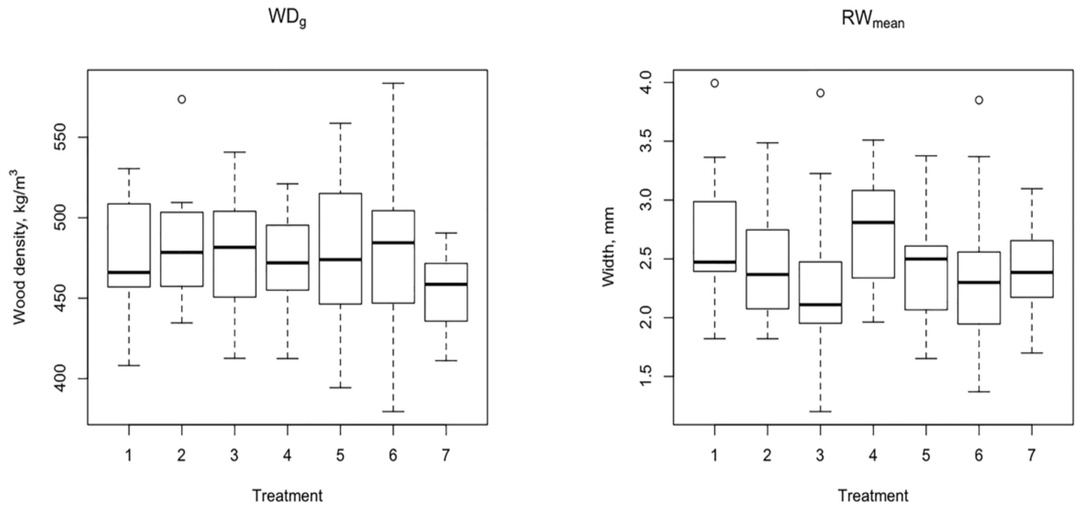
To answer the research questions and evaluate the hypotheses, the analysis was divided into two sections: (1) The variation of WD_g and RW_mean within different silvicultural treatments were assessed by evaluating data variation in boxplot figures that displays the distributional characteristics (i.e., the minimum, the maximum, the sample median, and the first and third quartiles) of each group and possible outliers. Then, a linear mixed-effects model (LME) in package nlme [48] of the R-software [47] was fitted and the analysis of variance was applied in testing the statistically significant differences in the mean wood density attributes (Equation (1)) between the silvicultural treatments to test the hypothesis H1.

y_ij = β_{1... 7} Treatment_k + a_i + c_ij + ϵ_ij

(1)

where y_ij is either WD_g or RW_mean, β₁,…β₇ are fixed parameters, Treatment_k is each silvicultural treatment (including control), i, i = 1, …, M, refers to study site, j, j = 1, …,n_i, to a plot, a_i and c_ij are normally distributed random effects for sample plot j and for sample plot j within study site i, respectively, with mean zero and unknown, unrestricted variance-covariance matrix, and ϵ_ij is a residual error with mean zero and unknown variance. The random effects are independent across study sites and sample plots as well as residual errors which are independent across trees. The effects of a study site and a sample plot within the study sites on the stem attributes were assessed through their variances.

(2) The dependencies between the structural characteristics and WD_g and RW_mean were first investigated based on Pearson’s correlation matrices in the R-software [47]. Then, an LME was fitted, and analysis of variance was applied similarly to the first phase of the analysis. Structural characteristics were added individually as explanatory variables to the fitted models shown in Equation (2). In addition, the fitted models were used to predict WD_g and RW_mean to assess the explanatory power of each structural characteristic through the coefficient of determination (R²) -value.

y_ij = β₁ Growth Characteristic_l + β_2...8 Treatment_k + a_i + c_ij + ϵ_ij

(2)

where y_ij is either WD_g or RW_mean, β₁,…β₈ are fixed parameters, Growth Characteristic_l is each structural characteristic described in Table 2, Treatment_k is each silvicultural treatment (including control), i, i = 1, …, M, refers to study site, j, j = 1, …,n_i, to a plot, a_i and c_ij are normally distributed random effects for sample plot j and for sample plot j within study site i, respectively, with mean zero and unknown, unrestricted variance-covariance matrix, and ϵ_ij is a residual error with mean zero and unknown variance.

3. Results

When evaluating the variation of WD_g between different silvicultural treatments (i.e., thinning type and intensity) to the control plot with no treatment, only a small increase in variation is visible in the box plot figures (Figure 2). The standard deviation of WD_g in the control plot was 27.2 kg/m³ in contrast to it varying between 33.1 kg/m³ to 47.7 kg/m³ depending on the thinning type and intensity (

Table 4. Statistics (minimum, maximum, mean and standard deviation) of ring basal area weighted mean wood density (WD_g) and mean ring width (RW_mean) between different thinning treatments. Moderate refers to thinning guidelines applied in Finland [43] whereas intensive results in 50% lower remaining basal area (m²/ha) compared to moderate thinning. Control refers to plots without thinning treatments since the establishment.

Forest Attribute	Statistics	Thinning from Below (Moderate/Intensive)	Thinning from Above (Moderate/Intensive)	Systematic Thinning (Moderate/Intensive)	Control
WDg (kg/m3)	Min	408.2/412.5	434.6/394.4	412.6/379.5	411.2
	Mean	478.3/473.1	480.4/476.9	476.5/480.6	451.7
	Max	530.5/521.1	573.6/558.7	540.8/583.6	490.5
	Std	33.6/31.3	33.1/45.1	35.7/47.7	27.2
RWmean (mm)	Min	1.8/2.0	1.8/1.7	1.2/1.4	1.7
	Mean	2.7/2.7	2.5/2.4	2.2/2.3	2.4
	Max	4.0/3.5	3.5/3.4	3.9/3.9	3.1
	Std	0.6/0.5	0.5/0.5	0.5/0.6	0.4

). Thinning intensity had a larger impact on the standard deviation of WD_g in thinning from above and systematic thinning, causing an increase of 33.6% to 36.3% in deviation compared to the thinning from below. Overall, the different silvicultural treatments caused a slight increase (21.4–28.9 kg/m³) in the average WD_g compared to the control plot. When evaluating the effect of different silvicultural treatments to RW_mean, results show that thinning from above and systematic thinning tended to decrease the RW_mean when compared to moderate thinning (Table 4). When compared to the control plots, all treatments resulted in slightly increased variation in RW_mean values.

The fitted linear mixed effects models (Equation (1)) and analysis of variance provided quantitative details about the significance of the effect of different silvicultural treatments on the WD_g and RW_mean. Analysis showed that the silvicultural treatments did not have a significant effect (p-values > 0.05) on WD_g. Similarly, only low (below 0.3) correlations were found between WD_g and structural characteristics (

Table 5. Pearson’s correlation coefficients between ring basal area weighted mean wood density (WD_g), mean ring width (RW_mean) and tree structural characteristics (refer to Table 2 for descriptions). * Indicates a statistical significance (i.e., p-value ≤ 0.05). ** Indicates a strong correlation (i.e., correlation > 0.5).

	WDg		RWmean
Characteristic	Correlation	p-Value	Correlation	p-Value
DBH	−0.04	0.67	0.61 **	0.00 *
H	0.16	0.08	0.27	0.00 *
V	−0.04	0.66	0.57 **	0.00 *
DBHgrowth	−0.09	0.31	0.56 **	0.00 *
Hgrowth	0.00	0.99	0.08	0.35
Vgrowth	−0.08	0.37	0.63 **	0.00 *
ggrowth	−0.07	0.42	0.65 **	0.00 *
CrownH	0.08	0.39	0.16	0.08
CrownWidth	0.06	0.49	0.42	0.00 *
CrownA	0.01	0.89	0.42	0.00 *
CrownVol	0.00	0.99	0.45	0.00 *
CrownLength	0.03	0.70	0.36	0.00 *
BranchDMean	0.10	0.28	−0.05	0.54
BranchDsd	−0.10	0.26	−0.03	0.74
Branch⍺mean	−0.24	0.01 *	0.07	0.40
Branch⍺sd	−0.10	0.27	0.00	0.99
WhorlDistmean	0.03	0.70	−0.16	0.06
WhorlDistsd	0.07	0.44	0.00	0.99
CI1	0.00	0.99	0.27	0.00 *
CI2	−0.13	0.14	0.49	0.00 *
CI3	0.13	0.15	0.16	0.08
CI4	0.13	0.13	0.13	0.15
CI5	0.12	0.16	0.08	0.39
CI6	0.11	0.21	0.10	0.25
CI7	−0.11	0.19	0.57 **	0.00 *
CI8	0.07	0.44	0.37	0.00 *
CI9	0.01	0.94	0.37	0.00 *
CI10	−0.04	0.62	0.39	0.00 *
CI11	−0.05	0.56	0.42	0.00 *

). In contrast, a p-value of 0.05 was found with RW_mean indicating that silvicultural treatments have a statistically significant effect on RW_mean. Pearson’s correlation analysis showed higher correlation values between RWmean and structural characteristics than WD_g. Statistical significant (i.e., p-value < 0.05) were found with following characteristics (Table 5): DBH, H, V, DBH_growth, V_growth, g_growth, Crown_Width, Crown_A, Crown_Vol, Crown_Length and competition indices C1–C2, C7–C11. The correlation values varied between 0.36 and 0.65 with these characteristics. The strongest correlations were for volume and basal-area growth.

Even though the LME-analysis showed that there was no statistically significant difference between silvicultural treatments, correlation tables showed a clear variability in the dependencies between the structural characteristics and WD_g within the treatments (Appendix A). When evaluating the correlation between structural characteristics and WD_g in moderate thinnings, negative correlation between −0.35 and −0.47 were found for DBH, H, V, g increment attributes for thinning from below but an opposite correlation between 0.23 to 0.34 was found in thinning from above. In contrast, no strong correlations (i.e., correlation > 0.5) between WD_g and crown characteristics (i.e., Crown_H, Crown_Width, Crown_A, Crown_Vol and Crown_Length) were found. In intensive treatments, the observed correlations were weaker in general. The highest correlation for intensive thinning from below and from above was found for Crown_H (0.53 and −0.41, respectively). The highest correlations between competition indices (i.e., CI1–11, see Table 2 for descriptions) and WD_g were found in the control plot (without any treatment) and the moderate systematic thinning. In the control plots, correlations of 0.37, 0.57 and 0.63 were found for CI1, CI3 and CI8, respectively. In the moderate systematic thinning, correlations between 0.43 and 0.44 were observed for CI4–CI6.

Treatment-wise correlations between RW_mean and structural characteristics were stronger in general compared to the corresponding values for WD_g (see Appendix A). Analysis showed moderate and strong correlations with statistically significant p-values (i.e., p-value < 0.05) within different thinning types and intensities. In general, the stronger correlations tended to be for DBH, V, DBH_growth, V_growth, g_growth and competition indices related to tree community (i.e., plot-level). Thinning from above tended to have lower correlations compared to thinning from below or systematic thinning. However, between intensive thinnings, this trend was not visible. The weakest correlations observed within the control plot were for g_growth (0.36).

To evaluate the statistical significance of each structural characteristic on the WD_g and RW_mean, LME models and analysis of variance were applied. The analysis showed (

Table 6. The p-values and coefficient of determination (R²) of the fitted linear mixed effects models (Equation (2)) and analysis of variance where ring basal area weighted mean wood density (WD_g) and mean ring width (RW_mean) were used as response variables and each tree structural characteristics (refer to Table 2 for descriptions) as predictor variables. * Indicates a statistical significance (i.e., p-value ≤ 0.05).

	WDg		RWmean
Characteristic	p-Value	R2	p-Value	R2
DBH	0.24	0.29	0.00 *	0.60
H	0.23	0.27	0.00 *	0.40
V	0.23	0.29	0.00 *	0.56
DBHgrowth	0.16	0.28	0.00 *	0.51
Hgrowth	0.31	0.29	0.52	0.21
Vgrowth	0.16	0.29	0.00 *	0.54
ggrowth	0.18	0.29	0.00 *	0.59
CrownH	0.52	0.27	0.03 *	0.25
CrownWidth	0.53	0.27	0.00 *	0.46
CrownA	0.15	0.30	0.00 *	0.46
CrownVol	0.16	0.30	0.00 *	0.48
CrownLength	0.49	0.28	0.00 *	0.38
BranchDMean	0.20	0.26	0.25	0.22
BranchDsd	0.42	0.27	0.90	0.21
Branch⍺mean	0.00 *	0.31	0.37	0.22
Branch⍺sd	0.41	0.27	0.66	0.21
WhorlDistmean	0.52	0.28	0.09	0.23
WhorlDistsd	0.31	0.29	0.91	0.21
CI1	0.10	0.31	0.00 *	0.32
CI2	0.08	0.30	0.00 *	0.54
CI3	0.42	0.27	0.00 *	0.28
CI4	0.56	0.27	0.00 *	0.28
CI5	0.56	0.26	0.01 *	0.26
CI6	0.65	0.26	0.01 *	0.26
CI7	0.16	0.28	0.00 *	0.56
CI8	0.50	0.27	0.00 *	0.38
CI9	0.57	0.27	0.00 *	0.43
CI10	0.24	0.28	0.00 *	0.43
CI11	0.26	0.28	0.00 *	0.45

) that traditional tree size (DBH, H and V) or structural characteristics (DBH_growth, H_growth, V_growth and g_growth) did not have a statistically significant effect (p-values > 0.05) on WD_g. A similar result is found for mean whorl to whorl distance (i.e., Whorl_Dmean) which is expected to be a good indicator of height growth for Scots pine trees. In contrast, when evaluating respective LME values for RW_mean, all the above-mentioned characteristics except Whorl_Dmean had a statistically significant effect. DBH, V, DBH_growth, V_growth and g_growth could explain 51%–60% of the variation of RW_mean. LME modelling also showed that none of the crown characteristics (i.e., Crown_H, Crown_Width, Crown_A, Crown_Vol and Crown_Length) had a statistically significant (p-values > 0.05) effect on WD_g. In contrast, analysis showed that all crown characteristics had a statistically significant effect (p-values < 0.05) on RW_mean. When evaluating R²-values (Table 6), crown characteristics explained the variation of RW_mean better compared to WD_g, in general. The highest R² value of 0.48 was found between RW_mean and Crown_Vol. When evaluating the branch characteristics, only the mean branch angle (i.e., Branch_ɑmean) was found to have significant effect (p-values < 0.05) on WD_g. In addition, the results show that the effect of competition indices (C1–C11) had no statistically significant effect (p-values > 0.05) for WD_g. However, statistically significant effects (p-values < 0.05) were found between all competition indices and RW_mean. The highest R² values were found for CI2 and CI7, which explained 54% or 56% of RW_mean variation.

4. Discussion

The main aim of this work was to evaluate the dependencies between TLS-derived structural characteristics of a Scots pine trees and internal wood properties. Evaluation focused on tree-specific WD_g and RW_mean properties at breast-height and analysis was conducted in a study area with varying silvicultural treatments. The first research question was to evaluate how the varying silvicultural treatments affect the wood properties in question. Results show that different thinning types or intensities did not have a statistically significant effect on WD_g. However, treatments did have a minor impact on treatment-wise variation in WD_g by increasing the mean values approximately 20–30 kg/m³ (~4.8–6.4%) when compared to the control plots. In addition, the standard deviation of WD_g increased approximately 15%–75% compared to the control plots. The highest increase in standard deviation was observed in intensive systematic thinning. The observed basic density values in our study were within the range reported in literature, but did not cover the full possible range: the wood density can range between 350 kg/m³ and 650 kg/m³, when within-tree variabilities are considered [15,49]. It should be noted that the minor increase in WD_g due to the treatments is not in line with previous research. In general, it is stated that thinning treatments will decrease the WD_g due to the increased growth but for example Jaakkola et al. [12] concluded that intensive thinning is required to have considerable effect on WD_g. The results are most likely affected by the short timeframe since the establishment (approximately 12–13 growing seasons) where the effect of increased growth did not have that significant effect on the overall WD_g of a tree or tree communities. Peltola et al. [13] also concluded that the nonsignificant effect on WD_g could be caused by the simultaneous decrease in early wood density and increase in late wood density. Another notable cause was the fact that the analysis focused on the whole life cycle of the sample trees instead of the time after the treatments. This was due to the wood density sampling process which was collected using drill samples where detection of year rings was insufficient due to the challenges in sample quality (cracks or other damages). Based on these results, the hypothesis H1 was rejected.

Previous research has indicated that silvicultural treatments have a significant effect on the radial growth (i.e., ring width) of trees [13,50]. Similar results were observed in this study as a statistically significant effect between treatments and RW_mean was observed. RW_mean increased especially in thinning from below due to the tree selection during treatment. In thinning from below, mainly small, suppressed, or codominant trees were removed, and the remaining dominant trees can fully utilize the increasing growth space. This was supported by the increase in DBH_growth (see Table 3) compared to the other treatments and control plots. Results also show that in systematic thinning, where only dominant trees were removed and small, suppressed trees were left to grow, RW_mean tended to decrease. In addition, all treatments resulted in slightly increased variation in RW_mean values compared to control plots.

The second research question was to evaluate what the most influential structural characteristics are that explain WD_g or RW_mean variation. Overall, the correlations between WD_g and structural characteristics were low (below 0.3) indicating that these tree-level characteristics derived in a single time point cannot explain the variability of WD_g. This was supported by the results of LME modeling showcasing the lack of statistically significant effect between structural characteristics and WD_g. Even though no statistically significant effect was observed between silvicultural treatments, treatment-wise correlations showed a clear variability in the interactions between the structural characteristics and WD_g. Notably stronger correlations were observed especially in thinning from below between the structural metrics describing the increment of DBH, H, V and g indicating that increased growth causes WD_g to decrease. In contrast, opposite correlations were observed in the thinning from above. This is most likely caused by the tree selection during the treatments and the trees’ capabilities to react to the increasing growth space (Scots pine being shade-intolerant, and high in crown-plasticity). Peltola et al. [13] observed that dominant trees had a higher absolute growth response to the treatments compared to suppressed trees. However, they also stated that if growth response is evaluated in relation to the tree size before treatment, suppressed trees had a higher relative growth response. In addition, Saarinen et al. [51] concluded that treatment type and intensity has an impact on stem size and shape of Scots pine trees in the same study area where this study was conducted. However, this increase in growth did not change the overall WD_g. In contrast to WD_g, the analysis results between RW_mean and structural characteristics were notably different. Moderate and strong correlations with statistically significant p-values (i.e., p-value < 0.05) within different thinning types and intensities were observed. This is supported by Peltola et al. [13] who observed an average of 9–20% increase in radial growth with intensive thinnings compared to moderate. The stronger correlations focused on the structural characteristics that are strongly related to the ring width such as DBH, V, DBH_growth, V_growth, g_growth.

Previously, the main focus has been on linking simple structural characteristics, such as radial growth to wood property variation [11,13,19,20] and detailed characterization of tree crowns or competition status have been neglected due to the limitation of conventional measurements. TLS point clouds have opened a novel possibility to evaluate the relationship between more detailed structural characteristics and wood property variation. Results observed in this study show that tree-specific crown characteristics and competition indices are not sufficient to explain the WD_g variation between trees. However, they had a statistically significant effect on RW_mean. The most influential crown characteristics were Crown_W, Crown_A and Crown_V. This result supports the idea that the increasing size of the tree crown may cause Scots pine trees to allocate their growth to increase the structural carrying capacity of the stem more than its water-conduction capacity. Competition indices C2 and C7 had the strongest correlation compared to the other indices. This result is logical as they illustrate the sample trees DBH in relation to the mean DBH of the closest trees or the sample plot. Results also indicate that the competition indices describing the competition status of a tree within the plot were more important than the competition with the closest trees. Based on these results, hypothesis H2 was partially confirmed. TLS point cloud-derived structural characteristics could explain the variability in RW_mean but not in WD_g.

5. Conclusions

Based on the results, it can be concluded that TLS point clouds can capture novel information relating crown structures and competition indices within tree communities and their interaction with wood properties, especially with RW_mean. Relating to WD_g, it remained impossible to relate the tree structure to wood density at tree-level (i.e., using mean value at breast height, and tree-level structural attributes). In further investigations, the inherent within-tree variations (e.g., the transition from juvenile to mature wood) should be further addressed. Moreover, as the current biomass and carbon calculations rely on rough mean density values, e.g., the forecasts of future forest biomass developments might be biased in the absence of values that depended on the tree age and size (i.e., within-tree factors). Our results also suggest that even tree-level mean values do not necessarily describe the full range of wood density variation. Information on the within-tree variabilities of the wood properties would also be crucial for the quality-oriented utilization of the timber. A multitude of ways remain to be studied to utilize TLS to comprehensively understand how the structural characteristics evolve in relation to the wood properties; e.g., utilizing ring-level wood property references accompanied by locally calibrated stem taper and branching functions, and exploring the prospects of TLS time series information, or those of the spatially substituted pseudo-time-series of trees at variable ages and sizes. In addition, improving the quality of wood density samples and optimizing the sample processing could further improve the analysis. Furthermore, new developments in point cloud processing especially relating to the branch and crown characteristics can improve the quality of these characteristics.

References

1. Saranpää, P. Wood Density and Growth. In Wood Quality and Its Biological Basis; CRC Press: Boca Raton, FL, USA, 2003. [Google Scholar]
2. Mäkinen, H.; Saranpää, P.; Linder, S. Wood-Density Variation of Norway Spruce in Relation to Nutrient Optimization and Fibre Dimensions. Can. J. For. Res. 2002, 32, 185–194. [Google Scholar] [CrossRef]
3. Jucker, T.; Bouriaud, O.; Coomes, D.A. Crown Plasticity Enables Trees to Optimize Canopy Packing in Mixed-Species Forests. Funct. Ecol. 2015, 29, 1078–1086. [Google Scholar] [CrossRef] [Green Version]
4. Huuskonen, S.; Hynynen, J.; Valkonen, S. Metsänkasvatus-Menetelmät Ja Kannattavuus; Metsäkustannus Oy: Helsinki, Finland, 2014; ISBN 978-952-6612-39-3. [Google Scholar]
5. Macdonald, E.; Hubert, J. A Review of the Effects of Silviculture on Timber Quality of Sitka Spruce. Forestry 2002, 75, 107–138. [Google Scholar] [CrossRef] [Green Version]
6. Moore, J.R.; Cown, D.J. Corewood (Juvenile Wood) and Its Impact on Wood Utilisation. Curr. For. Rep. 2017, 3, 107–118. [Google Scholar] [CrossRef]
7. Zhang, S.Y. Effect of Growth Rate on Wood Specific Gravity and Selected Mechanical Properties in Individual Species from Distinct Wood Categories. Wood Sci. Technol. 1995, 29, 451–465. [Google Scholar] [CrossRef]
8. Zobel, B. The Changing Quality of the World Wood Supply. Wood Sci. Technol. 1984, 18, 1–17. [Google Scholar] [CrossRef]
9. Barbour, R.J.; Fayle, D.C.; Chauret, G.; Cook, J.; Karsh, M.B.; Ran, S. Breast-Height Relative Density and Radial Growth in Mature Jack Pine (Pinus banksiana) for 38 Years after Thinning. Can. J. For. Res. 1994, 24, 2439–2447. [Google Scholar] [CrossRef]
10. Pape, R. Influence of Thinning and Tree Diameter Class on the Development of Basic Density and Annual Ring Width in Picea Abies. Scand. J. For. Res. 1999, 14, 27–37. [Google Scholar] [CrossRef]
11. Makinen, H.; Hynynen, J. Wood Density and Tracheid Properties of Scots Pine: Responses to Repeated Fertilization and Timing of the First Commercial Thinning. Forestry 2014, 87, 437–447. [Google Scholar] [CrossRef] [Green Version]
12. Jaakkola, T.; Mäkinen, H.; Saranpää, P. Wood Density in Norway Spruce: Changes with Thinning Intensity and Tree Age. Can. J. For. Res. 2005, 35, 1767–1778. [Google Scholar] [CrossRef]
13. Peltola, H.; Kilpeläinen, A.; Sauvala, K.; Räisänen, T.; Ikonen, V.P. Effects of Early Thinning Regime and Tree Status on the Radial Growth and Wood Density of Scots Pine. Silva Fenn. 2007, 41, 285. [Google Scholar] [CrossRef] [Green Version]
14. Ikonen, V.P.; Peltola, H.; Wilhelmsson, L.; Kilpeläinen, A.; Väisänen, H.; Nuutinen, T.; Kellomäki, S. Modelling the Distribution of Wood Properties along the Stems of Scots Pine (Pinus sylvestris L.) and Norway Spruce (Picea abies L. Karst.) as Affected by Silvicultural Management. For. Ecol. Manag. 2008, 256, 1356–1371. [Google Scholar] [CrossRef]
15. Auty, D.; Achim, A.; Macdonald, E.; Cameron, A.D.; Gardiner, B.A. Models for Predicting Wood Density Variation in Scots Pine. Forestry 2014, 87, 449–458. [Google Scholar] [CrossRef] [Green Version]
16. Auty, D.; Moore, J.; Achim, A.; Lyon, A.; Mochan, S.; Gardiner, B. Effects of Early Respacing on the Density and Microfibril Angle of Sitka Spruce Wood. Forestry 2018, 91, 307–319. [Google Scholar] [CrossRef]
17. Moore, J.R.; Cown, D.J.; McKinley, R.B.; Sabatia, C.O. Effects of Stand Density and Seedlot on Three Wood Properties of Young Radiata Pine Grown at a Dry-Land Site in New Zealand. N. Z. J. For. Sci. 2015, 45, 4. [Google Scholar] [CrossRef] [Green Version]
18. Piispanen, R.; Heinonen, J.; Valkonen, S.; Mäkinen, H.; Lundqvist, S.O.; Saranpää, P. Wood Density of Norway Spruce in Uneven-Aged Stands. Can. J. For. Res. 2014, 44, 136–144. [Google Scholar] [CrossRef]
19. Jyske, T.; Mäkinen, H.; Saranpää, P. Wood Density within Norway Spruce Stems. Silva Fenn. 2008, 42, 248. [Google Scholar] [CrossRef] [Green Version]
20. Mäkinen, H.; Hynynen, J. Predicting Wood and Tracheid Properties of Scots Pine. For. Ecol. Manag. 2012, 279, 11–20. [Google Scholar] [CrossRef]
21. Maas, H.G.; Bienert, A.; Scheller, S.; Keane, E. Automatic Forest Inventory Parameter Determination from Terrestrial Laser Scanner Data. Int. J. Remote Sens. 2008, 29, 1579–1593. [Google Scholar] [CrossRef]
22. Kankare, V.; Holopainen, M.; Vastaranta, M.; Puttonen, E.; Yu, X.; Hyyppä, J.; Vaaja, M.; Hyyppä, H.; Alho, P. Individual Tree Biomass Estimation Using Terrestrial Laser Scanning. ISPRS J. Photogramm. Remote Sens. 2013, 75, 64–75. [Google Scholar] [CrossRef]
23. Kankare, V.; Holopainen, M.; Vastaranta, M.; Liang, X.; Yu, X.; Kaartinen, H.; Kukko, A.; Hyyppä, J. Outlook for the Single-Tree-Level Forest Inventory in Nordic Countries. In Lecture Notes in Geoinformation and Cartography; Springer: Berlin/Heidelberg, Germany, 2017. [Google Scholar]
24. Saarinen, N.; Kankare, V.; Vastaranta, M.; Luoma, V.; Pyörälä, J.; Tanhuanpää, T.; Liang, X.; Kaartinen, H.; Kukko, A.; Jaakkola, A.; et al. Feasibility of Terrestrial Laser Scanning for Collecting Stem Volume Information from Single Trees. ISPRS J. Photogramm. Remote Sens. 2017, 123, 140–158. [Google Scholar] [CrossRef]
25. Liang, X.; Kankare, V.; Yu, X.; Hyyppä, J.; Holopainen, M. Automated Stem Curve Measurement Using Terrestrial Laser Scanning. IEEE Trans. Geosci. Remote Sens. 2014, 52, 1739–1748. [Google Scholar] [CrossRef]
26. Calders, K.; Newnham, G.; Burt, A.; Murphy, S.; Raumonen, P.; Herold, M.; Culvenor, D.; Avitabile, V.; Disney, M.; Armston, J.; et al. Nondestructive Estimates of Above-Ground Biomass Using Terrestrial Laser Scanning. Methods Ecol. Evol. 2015, 6, 198–208. [Google Scholar] [CrossRef]
27. Dassot, M.; Constant, T.; Fournier, M. The Use of Terrestrial LiDAR Technology in Forest Science: Application Fields, Benefits and Challenges. Ann. For. Sci. 2011, 68, 959–974. [Google Scholar] [CrossRef] [Green Version]
28. Liang, X.; Kankare, V.; Hyyppä, J.; Wang, Y.; Kukko, A.; Haggrén, H.; Yu, X.; Kaartinen, H.; Jaakkola, A.; Guan, F.; et al. Terrestrial Laser Scanning in Forest Inventories. ISPRS J. Photogramm. Remote Sens. 2016, 115, 63–77. [Google Scholar] [CrossRef]
29. Liang, X.; Hyyppä, J.; Kaartinen, H.; Lehtomäki, M.; Pyörälä, J.; Pfeifer, N.; Holopainen, M.; Brolly, G.; Francesco, P.; Hackenberg, J.; et al. International Benchmarking of Terrestrial Laser Scanning Approaches for Forest Inventories. ISPRS J. Photogramm. Remote Sens. 2018, 144, 137–179. [Google Scholar] [CrossRef]
30. Newnham, G.J.; Armston, J.D.; Calders, K.; Disney, M.I.; Lovell, J.L.; Schaaf, C.B.; Strahler, A.H.; Mark Danson, F. Terrestrial Laser Scanning for Plot-Scale Forest Measurement. Curr. For. Rep. 2015, 1, 239–251. [Google Scholar] [CrossRef] [Green Version]
31. Wilkes, P.; Lau, A.; Disney, M.; Calders, K.; Burt, A.; Gonzalez de Tanago, J.; Bartholomeus, H.; Brede, B.; Herold, M. Data Acquisition Considerations for Terrestrial Laser Scanning of Forest Plots. Remote Sens. Environ. 2017, 196, 140–153. [Google Scholar] [CrossRef]
32. Yrttimaa, T.; Saarinen, N.; Kankare, V.; Liang, X.; Hyyppä, J.; Holopainen, M.; Vastaranta, M. Investigating the Feasibility of Multi-Scan Terrestrial Laser Scanning to Characterize Tree Communities in Southern Boreal Forests. Remote Sens. 2019, 11, 1423. [Google Scholar] [CrossRef] [Green Version]
33. Kankare, V.; Joensuu, M.; Vauhkonen, J.; Holopainen, M.; Tanhuanpää, T.; Vastaranta, M.; Hyyppä, J.; Hyyppä, H.; Alho, P.; Rikala, J.; et al. Estimation of the Timber Quality of Scots Pine with Terrestrial Laser Scanning. Forests 2014, 5, 1879–1895. [Google Scholar] [CrossRef] [Green Version]
34. Saarinen, N.; Calders, K.; Kankare, V.; Yrttimaa, T.; Junttila, S.; Luoma, V.; Huuskonen, S.; Hynynen, J.; Verbeeck, H. Understanding 3D Structural Complexity of Individual Scots Pine Trees with Different Management History. Ecol. Evol. 2021, 11, 2561–2572. [Google Scholar] [CrossRef] [PubMed]
35. Pyorala, J.; Liang, X.; Vastaranta, M.; Saarinen, N.; Kankare, V.; Wang, Y.; Holopainen, M.; Hyyppa, J. Quantitative Assessment of Scots Pine (Pinus sylvestris L.) Whorl Structure in a Forest Environment Using Terrestrial Laser Scanning. IEEE J. Sel. Top. Appl. Earth Observ. Remote Sens. 2018, 11, 3598–3607. [Google Scholar] [CrossRef] [Green Version]
36. Pyörälä, J.; Saarinen, N.; Kankare, V.; Coops, N.C.; Liang, X.; Wang, Y.; Holopainen, M.; Hyyppä, J.; Vastaranta, M. Variability of Wood Properties Using Airborne and Terrestrial Laser Scanning. Remote Sens. Environ. 2019, 235, 111474. [Google Scholar] [CrossRef]
37. Hu, M.; Pitkänen, T.P.; Minunno, F.; Tian, X.; Lehtonen, A.; Mäkelä, A. A New Method to Estimate Branch Biomass from Terrestrial Laser Scanning Data by Bridging Tree Structure Models. Ann. Bot. 2021, 128, 737–752. [Google Scholar] [CrossRef] [PubMed]
38. Raumonen, P.; Kaasalainen, M.; Markku, Å.; Kaasalainen, S.; Kaartinen, H.; Vastaranta, M.; Holopainen, M.; Disney, M.; Lewis, P. Fast Automatic Precision Tree Models from Terrestrial Laser Scanner Data. Remote Sens. 2013, 5, 491–520. [Google Scholar] [CrossRef] [Green Version]
39. Pitkänen, T.P.; Raumonen, P.; Kangas, A. Measuring Stem Diameters with TLS in Boreal Forests by Complementary Fitting Procedure. ISPRS J. Photogramm. Remote Sens. 2019, 147, 294–306. [Google Scholar] [CrossRef]
40. Pitkänen, T.P.; Raumonen, P.; Liang, X.; Lehtomäki, M.; Kangas, A. Improving TLS-Based Stem Volume Estimates by Field Measurements. Comput. Electron. Agric. 2021, 180, 105882. [Google Scholar] [CrossRef]
41. Yrttimaa, T.; Saarinen, N.; Kankare, V.; Viljanen, N.; Hynynen, J.; Huuskonen, S.; Holopainen, M.; Hyyppä, J.; Honkavaara, E.; Vastaranta, M. Multisensorial Close-Range Sensing Generates Benefits for Characterization of Managed Scots Pine (Pinus sylvestris L.) Stands. ISPRS Int. J. Geo-Inf. 2020, 9, 309. [Google Scholar] [CrossRef]
42. Cajander, A.K. Ueber Die Waldtypen. Acta For. Fenn. 1909, 1, 1–175. [Google Scholar]
43. Äijälä, O.; Koistinen, A.; Sved, J.; Vanhatalo, K.; Väisänen, P. Metsänhoidon Suositukset; Tapio Oy: Helsinki, Finland, 2019. [Google Scholar]
44. Laasasenaho, J. Taper Curve and Volume Functions for Pine, Spruce and Birch. Commun. Inst. For. Fenn. 1982, 108, 1–74. [Google Scholar]
45. Yrttimaa, T. Automatic Point Cloud Processing Tools to Characterize Trees (Point-Cloud-Tools: V1.0.1); Zenodo: Geneva, Switzerland, 2021. [Google Scholar]
46. Silva, C.A.; Crookston, N.L.; Hudak, A.T.; Vierling, L.A.; Klauberg, C.; Cardil, A. rLiDAR: LiDAR Data Processing and Visualization. R Package Version 0. 2017, 1. Available online: https://github.com/carlos-alberto-silva/rLiDAR (accessed on 7 January 2022).
47. R Core Team. R: A Language and Environment for Statistical Computing. R Found. Stat. Comput. 2019. Available online: https://www.R-project.org/ (accessed on 17 January 2022).
48. Pinheiro, J.; Bates, D.; DebRoy, S.; Sarkar, D.; R Core Team. Nlme: Linear and Nonlinear Mixed Effects Models. R-Project. 2021. Available online: https://cran.r-project.org/web/packages/nlme/index.html (accessed on 15 March 2021).
49. Repola, J. Models for Vertical Wood Density of Scots Pine, Norway Spruce and Birch Stems, and Their Application to Determine Average Wood Density. Silva Fenn. 2006, 40, 322. [Google Scholar] [CrossRef] [Green Version]
50. Mäkinen, H.; Hynynen, J.; Penttilä, T. Effect of Thinning on Wood Density and Tracheid Properties of Scots Pine on Drained Peatland Stands. Forestry 2014, 88, 359–367. [Google Scholar] [CrossRef]
51. Saarinen, N.; Kankare, V.; Yrttimaa, T.; Viljanen, N.; Honkavaara, E.; Holopainen, M.; Hyyppä, J.; Huuskonen, S.; Hynynen, J.; Vastaranta, M. Assessing the Effects of Thinning on Stem Growth Allocation of Individual Scots Pine Trees. For. Ecol. Manag. 2020, 474, 118344. [Google Scholar] [CrossRef]
52. Saarinen, N.; Kankare, V.; Yrttimaa, T.; Viljanen, N.; Honkavaara, E.; Holopainen, M.; Hyyppä, J.; Huuskonen, S.; Hynynen, J.; Vastaranta, M. Detailed Point Cloud Data on Stem Size and Shape of Scots Pine Trees. bioRxiv 2020. [Google Scholar] [CrossRef]
53. Saarinen, N.; Kankare, V.; Huuskonen, S.; Hynynen, J.; Bianchi, S.; Yrttimaa, T.; Luoma, V.; Junttila, S.; Holopainen, M.; Hyyppä, J.; et al. Point Clouds from Terrestrial Laser Scanning from Crowns of Individual Scots Pine Trees; Zenodo: Geneva, Switzerland, 2021. [Google Scholar]
Figure 1. Location of three study sites namely Palomäki (62°3.6′ N 24°19.9′ E), Pollari (62°4.4′ N 24°30.1′ E) and Vesijako (61°21.8′ N 25°6.3′ E).
Forests 13 00397 g001
Figure 2. Boxplot figures for ring basal area weighted mean wood density (WDg) and mean ring width (RWmean) between different thinning treatments (i.e., moderate below (1), moderate above (2), moderate systematic (3), intensive below (4), intensive above (5), intensive systematic (6), no treatment (7)) showcasing the distributional characteristics (i.e., the minimum, the maximum, the sample median, and the first and third quartiles) of each group and possible outliers.
Forests 13 00397 g002