Communication

Accuracy of a LiDAR-Based Individual Tree Detection and Attribute Measurement Algorithm Developed to Inform Forest Products Supply Chain and Resource Management

by
Aaron M. Sparks
* and
Alistair M.S. Smith
Department of Forest, Rangeland and Fire Sciences, College of Natural Resources, University of Idaho, 875 Perimeter Drive, Moscow, ID 83844, USA
*
Author to whom correspondence should be addressed.
Forests 2022, 13(1), 3; https://doi.org/10.3390/f13010003
Submission received: 12 October 2021 / Revised: 17 December 2021 / Accepted: 19 December 2021 / Published: 21 December 2021
(This article belongs to the Section Forest Inventory, Modeling and Remote Sensing)

Abstract

:
Individual Tree Detection (ITD) algorithms that use Airborne Laser Scanning (ALS) data can provide accurate tree locations and measurements of tree-level attributes that are required for stand-to-landscape scale forest inventory and supply chain management. While numerous ITD algorithms exist, few have been assessed for accuracy in stands with complex forest structure and composition, limiting their utility for operational application. In this study, we conduct a preliminary assessment of the ability of the ForestView® algorithm created by Northwest Management Incorporated to detect individual trees, classify tree species, live/dead status, canopy position, and estimate height and diameter at breast height (DBH) in a mixed coniferous forest with an average tree density of 543 (s.d. ±387) trees/hectare. ITD accuracy was high in stands with lower canopy cover (recall: 0.67, precision: 0.8) and lower in stands with higher canopy cover (recall: 0.36, precision: 0.67), mainly owing to omission of suppressed trees that were not detected under the dominant tree canopy. Tree species that were well-represented within the study area had high classification accuracies (producer’s/user’s accuracies > ~60%). The similarity between the ALS estimated and observed tree attributes was high, with no statistical difference in the ALS estimated height and DBH distributions and the field observed height and DBH distributions. RMSEs for tree-level height and DBH were 0.69 m and 7.2 cm, respectively. Overall, this algorithm appears comparable to other ITD and measurement algorithms, but quantitative analyses using benchmark datasets in other forest types and cross-comparisons with other ITD algorithms are needed.

1. Introduction

Sustainable forest inventory and supply chain management relies on accurate and up-to-date information that describes the dynamic changes in composition, structure, and health of forest stands. This data is essential to accurately forecast growth and yield over large areas and where field inventory access is limited due to natural hazards or topography [1,2]. While on-the-ground field inventory has been the standard source of this information, remote sensing technologies such as airborne scanning Light Detection and Ranging (LiDAR), also referred to as Airborne Laser Scanning (ALS), can gather three-dimensional forest structural data over larger areas at a lower cost [3]. The three-dimensional mapping and laser return intensity information that ALS provides has since the mid 2000’s been demonstrated to enable precision forestry, or the ability to accurately identify and model tree-level attributes (e.g., live/dead status, height, stem diameter, age) needed for forest management decision making [1,2,4,5,6,7,8]. However, many challenges remain in tree-level data acquisition, including the difficulty of identifying individual trees and tree species in forests with complex composition and structure [9,10].
Individual Tree Detection (ITD), species determination, and measurement of structural attributes using ALS approaches have been long sought-after goals in precision forestry [11,12]. In operational forestry the majority of allometric relations used to model aboveground biomass, carbon stocks, and merchantable yield rely on diameter at breast height (DBH) and maximum tree heights [13], with limited studies only using maximum tree heights [14]. Multiple ITD algorithms have been developed with varying degrees of success. Many of the early methods focused on the semi-automatic detection of individual crown structural attributes such as maximum tree heights and diameters of individual tree crowns [12,15,16,17], while other studies focused on modelling canopy and stand attributes such as basal area and aboveground biomass [17,18]. These early studies exhibited challenges with operating under canopy closures exceeding 50% [9,19], not identifying small trees [17] and inferring biometrically important attributes such as DBH [19,20]. Although the accurate identification of individual tree species has always been considered the ‘holy grail’ in forestry remote sensing [21], most studies that have reported success incorporated both structural ALS and spectral datasets [22,23,24,25,26] or used ‘multi-spectral’ ALS datasets [27]. However, the integration or fusion of multiple remote sensing datasets brings with it a higher computational and analysis burden, likely limiting broad application by forestry land management writ large that may not have access to the necessary equipment or expertise; leading many to rely on proprietary ‘black-box’ products.
ITD approaches have included a wide array of semi-automatic and automatic methods and are described in multiple reviews [4,28,29,30,31]. These ITD methods have included using 2-dimensional wavelet analysis to detect tree locations, heights, and crown widths [9,12,16,19,32,33,34], detection of tree heights associated with a local height maxima and then using valley forming or region growing to delineate the crowns [35,36,37], associating tree crowns with clusters and a local density maximum [38], assessment of canopy cover and aggregates of crowns using object-oriented and geographic object-based image analysis methods [12,39], and using machine learning for characterizing the structural and species information of individual trees [40,41,42]. Although most approaches are focused on ITD, this information is often ultimately used within tree lists to describe distributions at stand or regional scales for use in forest growth and yield prediction software [7,17]. Although the lack of identification of small trees may not represent a significant quantity of instantaneous stand aboveground biomass or carbon [21], studies have sought their inclusion given their importance to the understanding of habitats and stand ingrowth [43]. The rate of ingrowth is critical information that is needed to model long-term forest products supply chain projections such as stand species composition, forest development, and potential harvest yield [43,44]. Notably, [17] described that recent studies have sought to approximate the distribution of these smaller trees through the assumption that the canopies represent a cluster of trees of varying sizes and not a single dominant tree [45].
Studies have used ALS intensity data to differentiate between different species and health status (e.g., presence of disease) and leaf-on versus leaf-off conditions as a route to assess individual species identification [2,46]. Other studies have used repeated ALS flights to assess relative growth or damage following disturbances [47,48]. Most recently, unmanned aerial vehicles (UAVs) and drones have been used to assess similar individual tree structural attributes as a potential lower cost alternative to ALS [49,50,51,52]. However, the delay that was observed between initial research applications and the widespread use of ALS in supporting operational forest products supply chains and resource management suggests that it may take at least a decade for UAV- and drone-based approaches to replace ALS as the standard approach to acquire these measurements [2,7].
The sustained interest in developing operational ALS methods that accurately assess individual tree attributes, species, and other important structural parameters has led to the development of a wide array of commercial and open-source solutions. Many of the commercial methods are proprietary (i.e., black box) and suffer from a lack of independent validation and verification [21,53]. However, as described in detail by [54], although multiple open-source ALS processing tools exist, many ‘free’ tools don’t share the underlying code (e.g., LAStools, FUSION) and others are dependent on specific operating systems or run with specific software packages (e.g., LidR [54]). Furthermore, it is likely that many small-medium sized forestry landowners will not have the expertise or available equipment to use these approaches and thus likely remain reliant on the reported accuracies of proprietary products. Although the adoption of freely available open-source methods is an idealized outcome, it remains essential for studies to objectively evaluate the different commercial proprietary approaches to provide end-users with independent and objective assessments of the suitability and accuracy of these products. Given the methodological steps of proprietary approaches are generally privileged information that are not shared in publications or publicly, the optimal approach to assess any method is through comparison of the derived structural and species metrics with independently analyzed robust field inventory datasets that can be assumed to represent ‘truth’ and capture a range of forest stand conditions and complexities [55].
The goal of the current study is to conduct a preliminary objective assessment of one of these commonly applied proprietary approaches: ForestView® that was developed by Northwest Management Incorporated (NMI, Moscow, Idaho). This method is widely used by private forestry landowners and has already been applied on approximately 4 million acres in 17 U.S. States and Canada, highlighting the timely need for an objective validation assessment. In conducting this assessment, the specific questions we sought to address are:
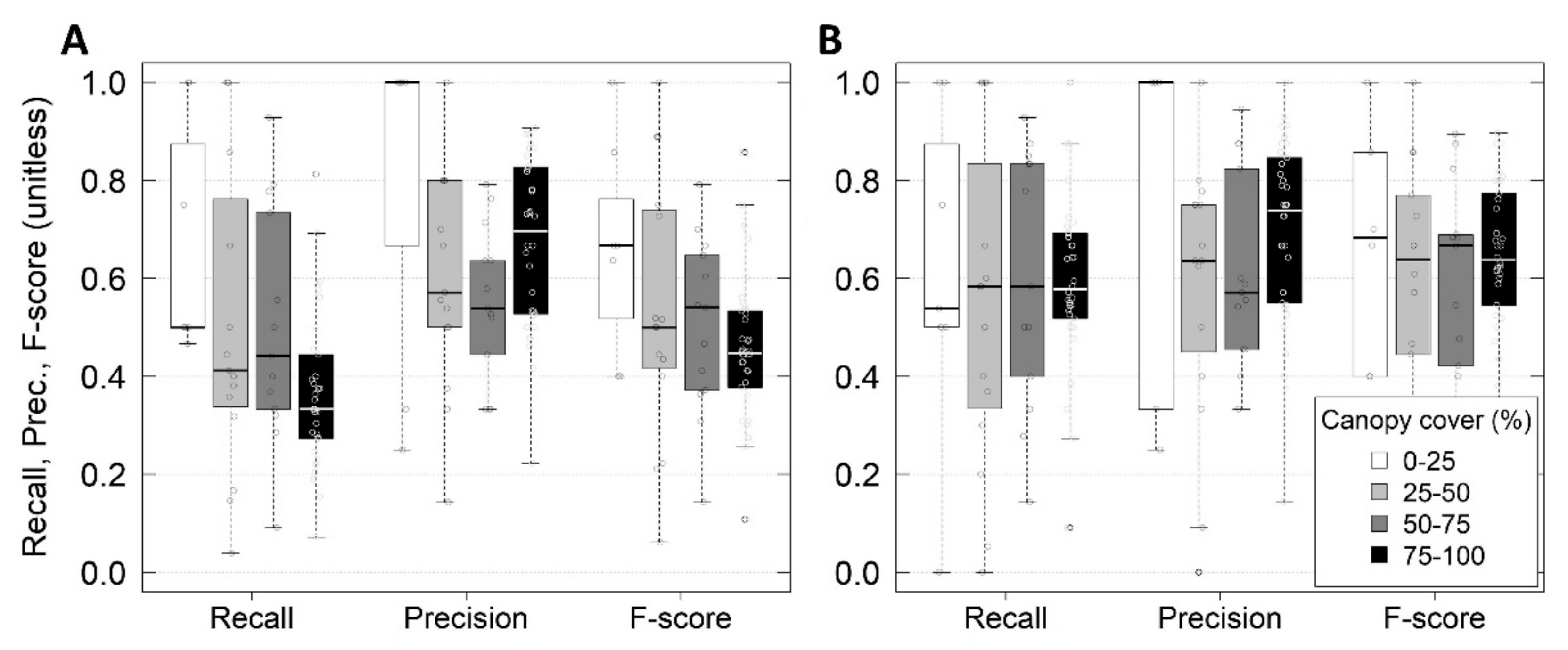
  • What is the ITD accuracy of this methodology and how does it vary with canopy cover?
  • How well does this methodology identify individual tree species, live/dead status, and canopy position?
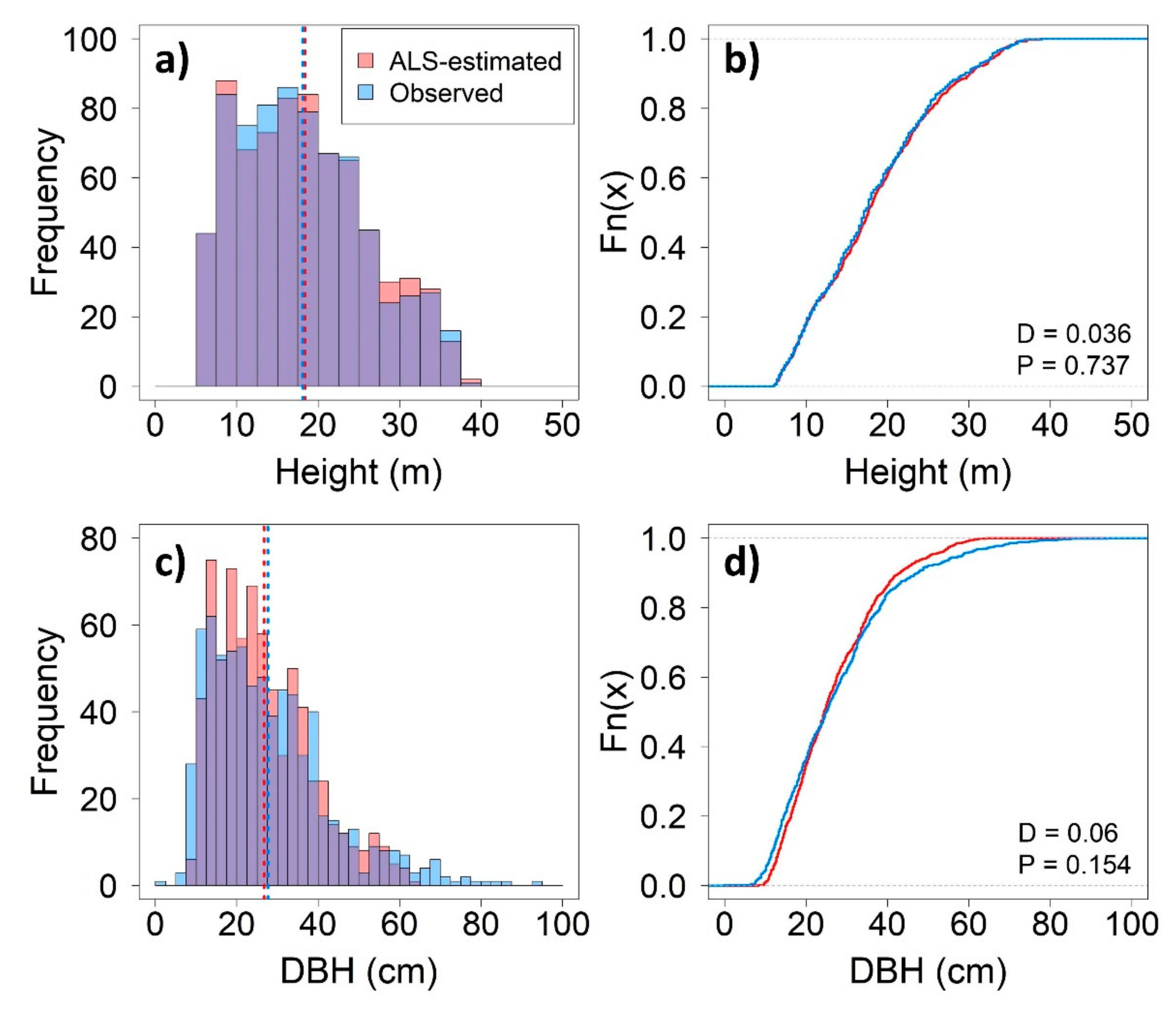
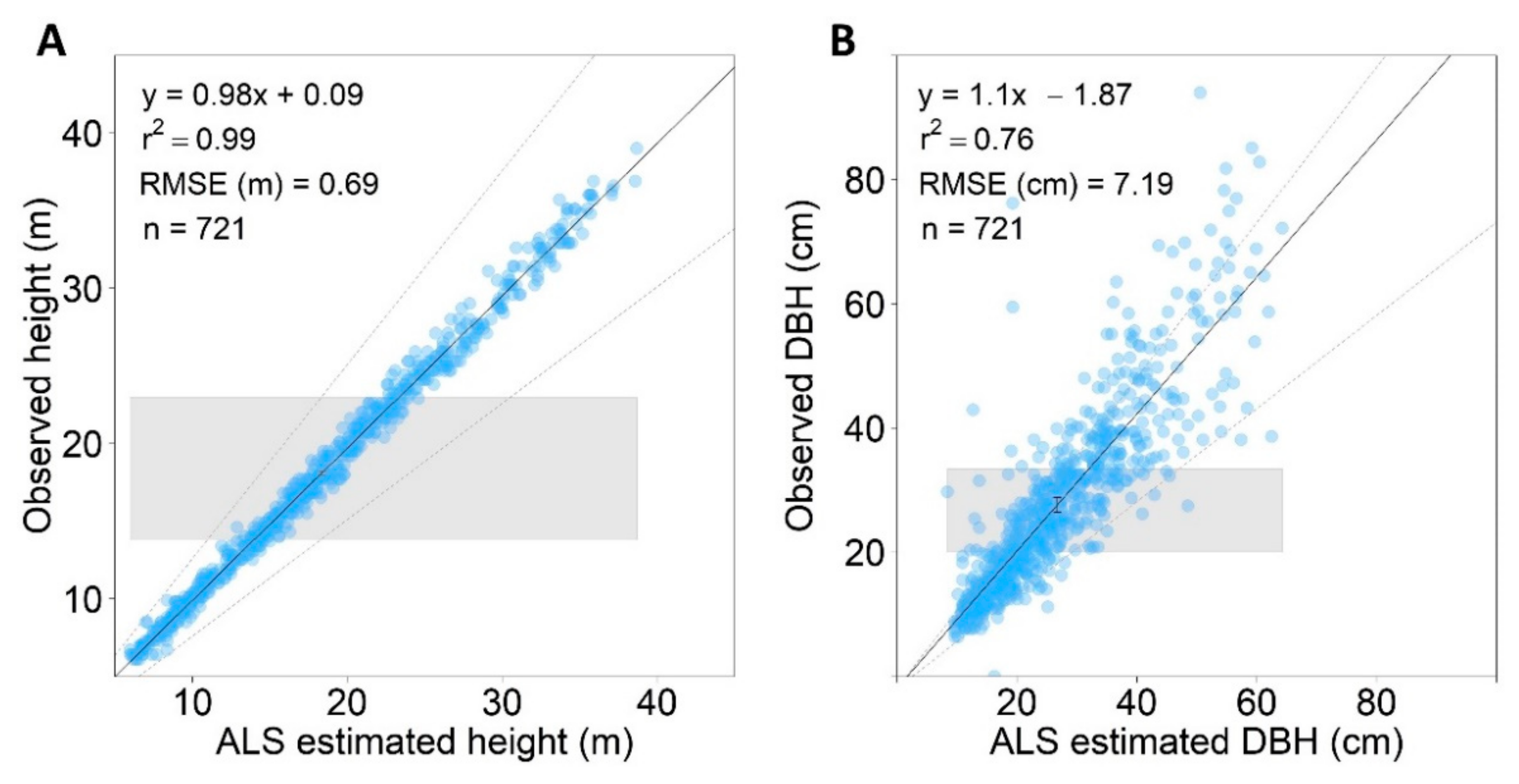
  • Are the maximum tree heights and DBH measurements obtained by this proprietary method statistically equivalent to field measurements?

2. Materials and Methods
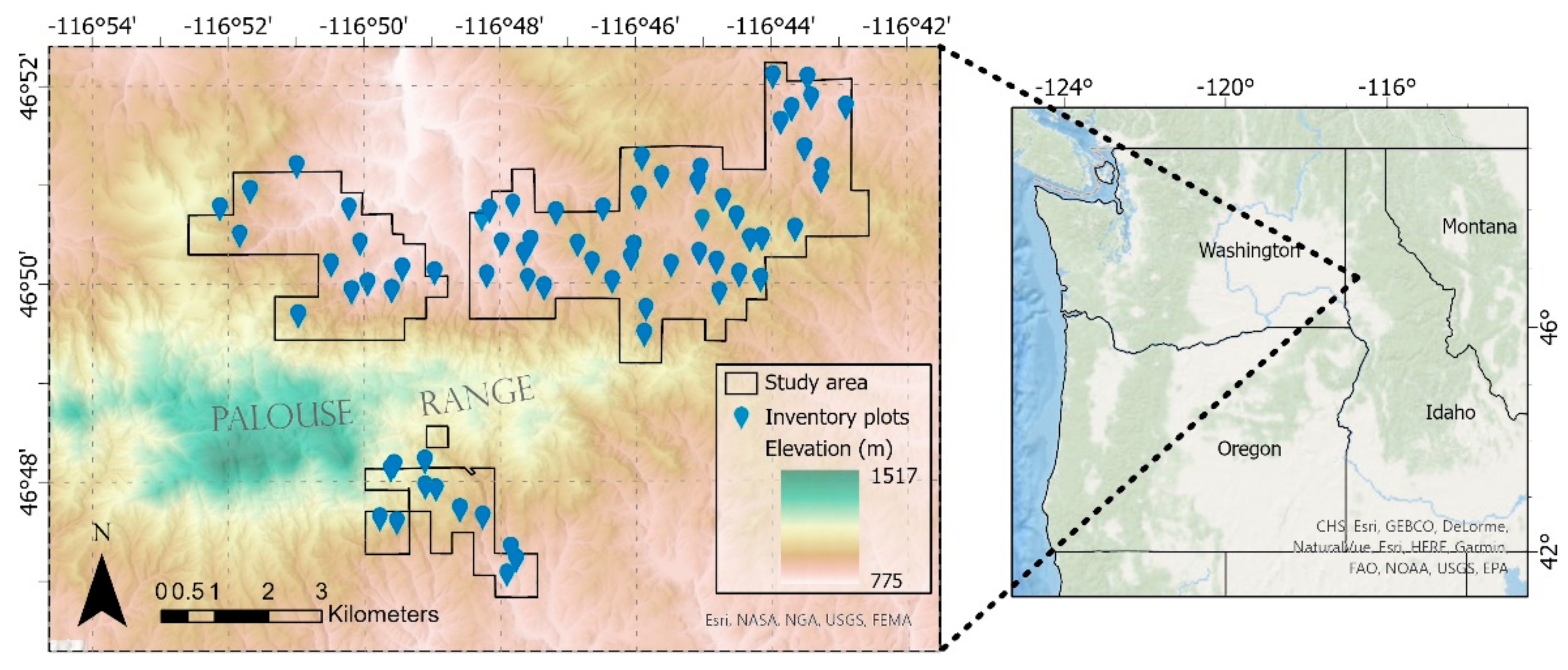
2.1. Study Area

This study was conducted on the University of Idaho Experimental Forest (UIEF), which is located on the Palouse Range in north-central Idaho, USA (Figure 1). The UIEF is a mixed-conifer temperate forest and dominant tree species include Pseudotsuga menziesii (Douglas-fir), Abies grandis (grand fir), Thuja plicata (western redcedar), and Larix occidentalis (western larch). Other species within the study area include Pinus ponderosa (ponderosa pine), Pinus contorta (lodgepole pine), Pinus monticola (western white pine), and Picea engelmannii (Engelmann spruce). The UIEF is actively managed for timber, research, and education purposes, and consequently has a diverse range of stand structures and composition. The UIEF has been used to objectively evaluate a variety of prior LiDAR products and algorithms [6,16,47].

2.2. Field Validation Dataset

In summer of 2020, 67 forest inventory plots, each having a 13 m radius and a 0.053-hectare area, were established via a stratified quasi-random sampling designed to sample the relationship between scanning data and individual tree structure and forest composition. This sampling density was chosen to represent the variability in forest structure and composition from the ALS point clouds. All plot locations were georeferenced using a Triumph-2 global navigation satellite system (JAVAD, San Jose) and Samsung Galaxy tablet with a Rover pole. The Triumph-2 is a rugged Bluetooth and WiFi enabled field mapping unit that enables real-time differential global positioning system recording with up to 2 GB of storage. All trees >1.5 m in height within the plot radius were stem-mapped using azimuth and distance from plot center using a Vertex Laser Geo 360 (Haglof, Sweden) and a 22.8 m forester’s tape. The Vertex Laser Geo 360 has a precision of 0.01 m, with a nominal accuracy of 0.04 m over a range of 700 m. Trees were measured for height, DBH, species, live/dead, crown width, crown height, stem taper, age, and canopy position (i.e., Dominant, Codominant, Intermediate, Suppressed). The Vertex, foresters’ tape, relaskop, and flagging to visually locate plot center, were used to collect field measurements and record them in a spreadsheet application on the Samsung tablets. A summary of tree measurements at the inventory plots is presented in Table 1.

2.3. ALS Data and Individual Tree Detection and Measurement Extraction

ALS data were acquired across the study area in the summer of 2019. These data were collected with a Riegl VQ-1560II sensor mounted in a fixed-wing aircraft and fitted with a Gryo Stabilized Mount. Elevation of the aircraft was maintained between 1600 and 1900 m above ground level and flight lines alternated orientations while maintaining a 50% flight-line overlap referencing the 58-degree FOV of the sensor. The average pulse density was 20 pulses per square meter (minimum of 16) with an average of greater than 4 returns per pulse over forested areas. Scanning data were preprocessed to normalize laser intensity within the Riegl RiPROCESS software and classified to bare earth, vegetation, water, buildings, and noise returns before being imported as LAZ files into ForestView®. Canopy cover for each plot was calculated as the number of ALS first returns above 1.37 m, divided by the total number of first returns.
Conversations with NMI provided the following information that they agreed to being included in this publication to help explain how the methodology operates without revealing proprietary information. The ForestView® system conducts a series of standard ALS pre-processing steps including development of multiple surface layers including a digital elevation model, digital surface model, and canopy height model, following standard approaches [56]. The system uses these layers alongside the original point cloud to infer structural metrics in a similar manner to other common ITD tools (e.g., [17,54,57]). ForestView® includes non-ALS data such as roads and property boundaries, in addition to ALS-derived metrics such as tree heights and canopy metrics, to stratify stands and units. ForestView® calculates a standard suite of ALS structural variables including heights, shapes, orientations, LiDAR intensities, and percentage of LiDAR returns broken up by vertical and horizontal strata and aggregates this data into 1/10th acre raster cells to interpret a project landscape into strata. ForestView® identifies stands in a similar manner to common segmentation approaches using heights and other structural metrics alongside ancillary information [12]. ForestView® assigns 1/10th acre field verification plot locations based on an analysis of the stand variability and then uses those ALS data associated with the individually detected trees at those ‘plots’ in the subsequent analysis. The ForestView® ITD algorithm follows common valley following and other watershed approaches [35,36,37], but shape and structural information associated with each ‘tree’ are used to identify species and further tune DBH, volume and canopy density metrics. The ForestView® software produces a suite of products including individual tree heights, DBH, total volume, canopy density, species identification, tree health and mortality. The software also provides the user with distribution tables for use in growth and yield models, a <0.5 m precision digital elevation model, road and trail layers, canopy and shade cover, and information related to fire risk, wildlife habitats, and forest productivity.

2.4. Matching ALS Detected and Reference Trees

Following [58], an automated approach was developed to match ALS detected trees and reference trees (i.e., field validation dataset). For each ALS detected tree, reference trees within a buffer distance ≤ 2.5 m were selected as candidate trees to be matched with the ALS detected tree. This buffer distance was chosen as it represents the average crown diameter of dominant and codominant trees on the Palouse Range [9]. The difference in height between the ALS detected tree and all candidate reference trees was calculated and all candidate reference trees with a height difference > 2 m were removed from the candidate tree list. The height difference threshold of 2 m corresponds to observed RMSE in height between ALS estimated and field measured conifers [59]. If no reference trees met the height difference threshold, the ALS detected tree was recorded as a commission error. For reference trees that did meet the height difference threshold, the difference between the ALS detected tree distance to plot center and all candidate reference tree distances to plot center was calculated. The reference tree with the smallest combined error (height difference and difference in distance from plot center), was matched with the ALS detected tree. Combined error was calculated as the square root of the sum of the squared errors. If multiple reference trees had the same combined error, we randomly selected one to match to the ALS detected tree.

2.5. Accuracy Assessment

Individual tree detection accuracy was evaluated using standard metrics that capture commission and omission errors. Specifically, recall (r), precision (p), and F-score [60] were used:
r = TP TP + FN
p = TP TP + FP
F - score = 2 × r × p r + p
where, TP = correct detection, FN = false negative (omission error), and FP = false positive (commission error). Recall is inversely related to omission error, precision is inversely related to commission error, and F-score is the harmonic mean of recall and precision. All three metrics range from 0 to 1, with values closer to 1 representing higher accuracy. Two sets of accuracy metrics were calculated; one set included all trees within the inventory plots, and the other only included trees in the dominant and codominant canopy positions. As prior studies have shown that tree detection accuracy generally decreases with increasing canopy cover [9], the plot-level accuracy results were stratified into four canopy cover classes (0–25%, 25–50%, 50–75%, 75–100%) to evaluate how detection accuracy changes with these increasing canopy cover strata. We assessed species, live/dead, and canopy position classification accuracy using confusion matrices calculated between the validation dataset and the ALS classification result. Three commonly used classification accuracy metrics (overall accuracy, producer’s accuracy, user’s accuracy) are reported.
We employed several statistical tests to assess whether ALS estimated tree attributes were statistically similar to field observed tree attributes for the matched ALS and reference trees. A Kolmogorov–Smirnov test was used to assess whether the ALS estimated height and DBH distributions were statistically similar to field observed height and DBH distributions. The Kolmogorov–Smirnov test computes differences in the cumulative distribution function of two data distributions, where the test statistic (D) symbolizes the point of maximum discrepancy in the cumulative distribution functions. D values closer to 0 indicate significant overlap in the data distributions and values closer to 1 indicate little to no overlap in the data distributions. This test is useful for quantifying the shape similarity of two distributions as two distributions with the same mean but significantly different shapes will produce large D values.
We evaluated the accuracy of modeled tree height and DBH using regression-based equivalence tests [61]. Equivalence tests have been widely applied in forest allometry to assess if significant differences exist between two sample populations that describe the same parameter, such as often occurs when comparing remote sensing metrics to field-measured validation data [9,34,61,62,63,64,65,66,67]. Following [61], we tested for both the intercept and slope equality between the paired sets of both DBH and maximum height measures. This test examines regression intercept equality (i.e., the mean of the ALS estimated measurement is equal to the mean of the field measurement) and slope equality to 1 (i.e., if ALS estimated measurements are equal to field measurements, regression will have slope of 1). Following [9,34,61,64], the region of equivalence is set to ±25% (of the mean) for the intercept and ±25% for the slope, where the null hypothesis of dissimilarity between the pairs of remotely sensed and field measurements of the same parameter are rejected if the interval of equivalence contains two joint one-sided 95% confidence intervals for the slope or the intercept. All statistical analyses were conducted in R [68], and equivalence tests were computed using the ‘equivalence’ R package [69].

3. Results

3.1. Individual Tree Detection Accuracy

The individual tree detection results are shown in Figure 2, considering all trees (Figure 2A), and only considering dominant and codominant trees (Figure 2B). Recall varied from 0.04 to 1, with a median value of 0.4 and average value of 0.45. Recall generally decreased with greater canopy cover, where recall was highest in plots with 0–25% canopy cover (median: 0.50, average: 0.67) and lowest in plots with 75–100% canopy cover (median: 0.33, average: 0.36). Precision varied from 0.14 to 1, with a median value of 0.67 and average value of 0.65. F-score varied from 0.06 to 1, with a median value of 0.47 and average value of 0.5. F-score also decreased with greater canopy cover (Figure 2A). The distribution of correct detections (TP) and false negatives (FN) by tree canopy position is shown in Figure 3. Most correct detections consisted of trees classified in the field as dominant or codominant. Conversely, most omission errors consisted of trees classified in the field as intermediate or suppressed.
ITD accuracy metrics generally increased when considering only trees with dominant and codominant canopy position (Figure 2B). Recall varied from 0 to 1, with a median value of 0.58, and average value of 0.59. Precision varied from 0 to 1, with a median value of 0.67 and average value of 0.66. F-score varied from 0.07 to 1, with a median value of 0.67 and average value of 0.62.

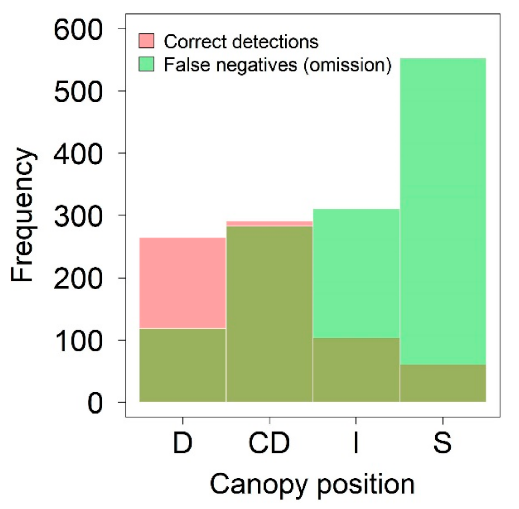
3.2. Species, Live/Dead, and Canopy Position Classification Accuracy

Species classification accuracy is presented in Table 2. Overall accuracy was 54.7% and individual species accuracy varied widely. Abies grandis, Pinus contorta, and Pinus ponderosa had the highest producer’s accuracies (60.6%, 68.4%, 65.9%, respectively) and user’s accuracies (60.0%, 56.5%, 78.8%, respectively), indicating relatively low omission and commission errors. Pinus monticola and Picea engelmannii had the lowest producer’s (0%) and user’s (0%) accuracies.
Live/dead classification accuracy is presented in Table 3. Overall accuracy was 97.4%, with high producer’s and user’s accuracies (>65%).
Tree canopy position classification accuracy is presented in Table 4. Overall accuracy was 74.0%, with high producer’s (>65%) and user’s accuracies (>51%).

3.3. Height and DBH Accuracy

The distribution of ALS estimated and observed height and DBH for all matched trees is shown in Figure 4. The Kolmogorov–Smirnov test statistic D was close to 0 for both height (D = 0.036, P = 0.737) and DBH (D = 0.06, P = 0.154), indicating no statistical difference between the ALS estimated and observed distributions. Figure 5 presents results from the statistical equivalence tests. For both height and DBH, the 95% confidence interval for the intercept (grey vertical bar) was within the ±25% region of equivalence (grey polygon). This means that the null hypothesis of dissimilarity can be rejected and that the ALS estimated means are equivalent to the field-measured means. Likewise, for both height and DBH, the 95% confidence interval for the slope (black vertical bar) was within the ±25% region of equivalence (grey dashed lines). This indicates that the regression fit slope is significantly similar to 1 (i.e., ALS estimated measurements are equivalent to field measurements). The linear relationship between ALS estimated height and observed height had a high r2 (0.99) and RMSE of 0.69 m. The linear relationship between ALS estimated DBH and observed DBH had a high r2 (0.76) and RMSE of 7.19 cm.

4. Discussion

This study objectively assessed the accuracy of the ForestView® algorithm for individual tree detection, classification, and measurement of tree height and DBH. Generally, ITD accuracy, as measured by F-score, was inversely related to canopy cover (Figure 2A). This result is consistent with results observed in prior studies under a range of different forest types [9,58,70]. The overwhelming majority of omission errors (reference trees not detected by the algorithm) were classified as Intermediate or Suppressed in the field validation dataset (Figure 3). This is a common issue in ITD as trees in subdominant canopy positions (e.g., intermediate and suppressed) are occluded by the overstory forest canopy [3,71]. Indeed, F-score values increased significantly when only considering dominant and codominant trees, especially in the highest canopy cover stratification (median F-score increased from 0.44 to 0.63) (Figure 2).
The detection accuracy results in this study are comparable to results obtained in prior studies looking at mixed coniferous forest with similar canopy cover and tree densities. For example, [72] reported detection of 40% of all trees in a mixed coniferous forest in Finland with a median tree density of 675 trees/hectare. Yancho et al. [73] tested several ITD algorithms using input digital aerial photogrammetric point clouds in mixed coniferous forest with a median tree density of 316 trees/hectare in British Columbia, Canada. They reported F-scores ranging from 0.568 to 0.609, with the highest F-score incorporating spectral and spatial attributes. Prior studies have achieved higher ITD accuracies in less dense coniferous forests. For example, [60] reported F-scores ranging from 0.83 to 0.95 in mixed coniferous forest with a median tree density of 300 trees/hectare in the Sierra Nevada Mountains in California. Silva et al. [58] achieved F-scores ranging from 0.79 to 1, in longleaf pine forests with stand densities ranging from 77–204 trees/hectare.
Individual tree species classification accuracy was highly variable (Table 2). This variation could be partly due to imbalance in species representation in the study area. Generally, species with the highest producer’s and user’s accuracy (Abies grandis, Pseudotsuga menziesii, Pinus contorta, and Pinus ponderosa) were well-represented in the field dataset, composing 31.3%, 22.2%, 5.1% and 11.1%, respectively, of the field dataset. Conversely, species with the lowest producer’s and user’s accuracy (Larix occidentalis, Picea engelmanii, Pinus monticola, and Thuja plicata) were less represented in the field tree dataset, composing 7.4%, 1.0%, 3.3% and 18.4%, respectively, of the field dataset. For machine learning classification algorithms, it is common for poorly represented classes in the training dataset to exhibit lower classification accuracy and this issue can be partly remediated by selecting a more balanced training dataset [74]. Equally, use of spectral or additional ALS data in winter could enable rapid identification of species with clear seasonal phenological leaf-off differences (i.e., Larix occidentalis). Nevertheless, species classification accuracies for the highly represented species in this study were comparable with other studies. For example, [75] reported species classification accuracies (producer’s and user’s) of 74–97% in a mixed coniferous and hardwood forest in Germany with a median stand density of 435 trees/hectare. Likewise, [76] reported accuracies of 75–90% for coniferous trees in a mixed conifer and hardwood forest in Finland. In southeastern deciduous forests, species identification accuracies of ~65% have been reported [77], a result that broadly agrees with a study focused on Central European forests [78]. When considering broader forest classifications such as the identification of broadleaved versus coniferous species, higher accuracies from 77–90% have been reported in an array of forested ecosystems [79].
Live/dead and canopy position classification had high overall accuracies (97.4% and 74%, respectively). High live/dead classification accuracy was expected given the widely documented large differences between live and dead LiDAR return pulse intensity [80]. The high accuracy of canopy position classification is encouraging for forest products supply chain and resource management considerations as it may facilitate harvest planning and scheduling. The accurate detection and classification of subdominant trees (e.g., intermediate and suppressed) is particularly promising, as the low overall detection of these trees (Figure 3) is clearly a limitation of current individual tree detection algorithms.
The similarity between the ALS estimated and observed tree attributes was high. The equivalence tests demonstrated that both the ForestView® algorithm-derived height and DBH were statistically equivalent to field-based measurements (Figure 5). Furthermore, the height RMSE of 0.69 m is comparable to other reported RMSEs including that reported by [59] in a Scots pine forest (1–1.3 m), [81] in a Scots pine forest (0.38 m), [75] in mixed conifer and hardwood forest (0.5–2.6 m) and by [58] in longleaf pine forest (0.72 m). The DBH RMSE of 7.2 cm obtained using the algorithm is higher than that obtained by [59] in a Scots pine forest (3.2–5.9 cm), [81] in a Scots pine forest (1.25 cm) and [75] in mixed conifer and hardwood forest (1.4–6.3 cm). There was no statistical difference in the ALS estimated height and DBH distributions and the field observed height and DBH distributions (Figure 4), indicating the broad applicability of these data in growth and yield projection software that rely on such distribution data such as the widely used Forest Vegetation Simulator [82]. The slight differences between the field and ITD derived data can be somewhat attributed to the difference in acquisition dates (i.e., ALS data in 2019 and field data in 2020). Although we assumed that the field data represented the ‘truth’, studies comparing both ALS and laser rangefinder maximum tree height measurements with felled trees have demonstrated that ALS measurements were more accurate and exhibited less bias [14].

5. Conclusions

The current study sought to evaluate the ForestView® ITD and measurement algorithm in comparison to field data to provide land management users of these products an objective assessment of this products accuracy. Overall, the analysis determined that this method produced comparable estimates of height and DBH to prior studies that reported on similar ‘open source’ and ‘free closed source’ methods. The approach does provide strong assessments of species identification and dominant/co-dominant assessment for half of the assessed species, where we posit the limitations were due to insufficient representation in the training dataset. As with prior studies, the method performs well in canopy cover strata < 75% but also performs strongly in the 75–100% canopy cover strata when solely considering dominant and co-dominant trees. Given these compelling preliminary results of the ForestView® algorithm, the next logical steps are to cross-compare this specific algorithm versus open-source and ‘free closed source algorithms’ in a similar manner to that conducted by [83]. Equally, further research should follow [14,47,83] to assess the utility of this algorithm to inform landscape scale assessments of forest stand metrics (e.g., basal area, trees per hectare) and projections of growth and yield. Further research could also explore the utility of this product to inform structural metrics of fire severity [48,84,85] and ecosystem vulnerability under a range of stressors [86]. With the recent publication of open-source, multi-sensor (e.g., LiDAR, high-resolution hyperspectral imagery) benchmark datasets that include numerous forest types and structures [87] there are even more opportunities to evaluate existing algorithms on a standard dataset.

Author Contributions

Conceptualization, A.M.S. and A.M.S.S.; methodology, A.M.S. and A.M.S.S.; formal analysis, A.M.S.; writing—original draft preparation, A.M.S. and A.M.S.S.; writing—review and editing, A.M.S. and A.M.S.S. All authors have read and agreed to the published version of the manuscript.

Funding

The authors received no form of funding or compensation from Northwest Management Incorporated to conduct this research.

Data Availability Statement

ALS algorithm outputs were provided freely by Northwest Management Incorporated (NMI) for use in this objective assessment. Groups interested in conducting similar analyses should contact NMI directly for data access.

Conflicts of Interest

The authors declare no conflict of interest.

References

  1. Evans, J.S.; Hudak, A.T.; Faux, R.; Smith, A.M.S. Discrete Return lidar in Natural Resources: Recommendations for Project Planning, Data Processing, and Deliverables. Remote Sens. 2009, 1, 776–794. [Google Scholar] [CrossRef] [Green Version]
  2. Hudak, A.T.; Evans, J.S.; Smith, A.M.S. Review: LiDAR Utility for Natural Resource Managers. Remote Sens. 2009, 1, 934–951. [Google Scholar] [CrossRef] [Green Version]
  3. White, J.C.; Coops, N.C.; Wulder, M.A.; Vastaranta, M.; Hilker, T.; Tompalski, P. Remote sensing technologies for enhancing forest inventories: A review. Can. J. Remote Sens. 2016, 42, 619–641. [Google Scholar] [CrossRef] [Green Version]
  4. Hyyppä, J.; Hyyppä, H.; Leckie, D.; Gougeon, F.; Yu, X.; Maltamo, M. Review of methods of small-footprint airborne laser scanning for extracting forest inventory data in boreal forests. Int. J. Remote Sens. 2008, 29, 1339–1366. [Google Scholar] [CrossRef]
  5. Smith, A.M.S.; Wynne, R.; Coops, N. Preface: Special issue on the Remote Characterization of Vegetation Structure and Productivity: Plant to Landscape Scales. Can. J. Remote Sens. 2008, 34, S3–S4. [Google Scholar] [CrossRef]
  6. Falkowski, M.J.; Hudak, A.T.; Crookston, N.; Gessler, P.E.; Ubeler, E.H.; Smith, A.M.S. Landscape-scale parameterization of a tree-level forest growth model: A k-NN imputation approach incorporating LiDAR data. Can. J. For. Res. 2010, 40, 184–199. [Google Scholar] [CrossRef]
  7. Tinkham, W.T.; Mahoney, P.R.; Smith, A.M.S.; Falkowski, M.J.; Woodall, C.; Donke, G.; Hudak, A.T. Applications of the United States Forest Service Forest Inventory and Analysis dataset: A review and future directions. Can. J. For. Res. 2018, 48, 1251–1268. [Google Scholar] [CrossRef]
  8. Goodbody, T.R.; Coops, N.C.; Luther, J.E.; Tompalski, P.; Mulverhill, C.; Frizzle, C.; Fournier, R.; Furze, S.; Herniman, S. Airborne laser scanning for quantifying criteria and indicators of sustainable forest management in Canada. Can. J. For. Res. 2021, 51, 972–985. [Google Scholar] [CrossRef]
  9. Falkowski, M.J.; Smith, A.M.S.; Gessler, P.E.; Hudak, A.T.; Vierling, L.A. The influence of conifer forest canopy cover upon the accuracy of two individual tree measurement algorithms using lidar data. Can. J. Remote Sens. 2008, 34, S338–S350. [Google Scholar] [CrossRef]
  10. Holopainen, M.; Vastaranta, M.; Hyyppä, J. Outlook for the next generation’s precision forestry in Finland. Forests 2014, 5, 1682–1694. [Google Scholar] [CrossRef] [Green Version]
  11. Hyyppa, J.; Inkinen, M. Detecting and estimating attributes for single tree using laser scanner. Photogramm. J. Finl. 1999, 16, 27–42. [Google Scholar]
  12. Smith, A.M.S.; Strand, E.K.; Steele, C.M.; Hann, D.B.; Garrity, S.R.; Falkowski, M.J.; Evans, J.S. Pro-duction of vegetation spatial-structure maps by per-object analysis of juniper encroachment in multi-temporal aerial photographs. Can. J. Remote Sens. 2008, 34, S268–S285. [Google Scholar] [CrossRef] [Green Version]
  13. Ter-Mikaelian, M.T.; Korzukhin, M.D. Biomass equations for sixty-five North American tree species. For. Ecol. Manag. 1997, 97, 1–24. [Google Scholar] [CrossRef] [Green Version]
  14. Tinkham, W.T.; Smith, A.M.S.; Affleck, D.; Saralecos, J.D.; Falkowski, M.J.; Hoffman, C.M.; Hudak, A.T.; Wulder, M.A. Development of height-volume relationships in second growth Abies grandis for use with aerial LiDAR. Can. J. Remote Sens. 2016, 42, 400–410. [Google Scholar] [CrossRef]
  15. Popescu, S.C.; Wynne, R.H. Seeing the Trees in the Forest: Using Lidar and Multispectral Data Fusion with Local Filtering and Variable Window Size for Estimating Tree Height. Photogram. Eng. Remote Sens. 2004, 16, 589–604. [Google Scholar] [CrossRef] [Green Version]
  16. Falkowski, M.J.; Smith, A.M.S.; Hudak, A.T.; Gessler, P.E.; Vierling, L.A.; Crookston, N.L. Automated estimation of individual conifer tree height and crown diameter via Two-dimensional spatial wavelet analysis of lidar data. Can. J. Remote Sens. 2006, 32, 153–161. [Google Scholar] [CrossRef] [Green Version]
  17. Jeronimo, S.M.A.; Kane, V.R.; Churchill, D.K.; McGaughey, R.J.; Franklin, J.F. Applying LiDAR Individual Tree Detection to Management of Structurally Diverse Forest Landscapes. J. For. 2018, 116, 336–346. [Google Scholar] [CrossRef] [Green Version]
  18. Hudak, A.T.; Crookston, N.L.; Evans, J.S.; Falkowski, M.J.; Smith, A.M.S.; Gessler, P.E.; Morgan, P. Regression modeling and mapping of coniferous forest basal area and tree density from discrete-return lidar and multispectral data. Can. J. Remote Sens. 2006, 32, 126–138. [Google Scholar] [CrossRef]
  19. Poznanovic, A.J.; Falkowski, M.J.; MacLean, A.L.; Evans, J.S.; Smith, A.M.S. An accuracy assessment of tree detection algorithms in juniper woodlands. Photogram. Eng. Remote Sens. 2014, 80, 45–55. [Google Scholar] [CrossRef]
  20. Andersen, H.-E.; Reutebuch, S.E.; McGaughey, R. A rigorous assessment of tree height measurements obtained using airborne lidar and conventional field methods. Can. J. Remote Sens. 2006, 32, 355–366. [Google Scholar] [CrossRef]
  21. Smith, A.M.S.; Greenberg, J.; Vierling, L.A. Introduction to Special Section: The Remote Characterization of Vegetation Structure: New methods and applications to landscape-regional-global scale processes. J. Geophys. Res. 2008, 113, 3–91. [Google Scholar] [CrossRef] [Green Version]
  22. Holmgren, J.; Persson, A.; Soderman, U. Species identification of individual trees by combining high resolution LiDAR data with multi-spectral images. Int. J. Remote Sens. 2008, 29, 1537–1552. [Google Scholar] [CrossRef]
  23. Dinuls, R.; Erins, G.; Lorencs, A.; Mednieks, I.; Sinica-Sinavskis, J. Tree Species Identification in Mixed Baltic Forest Using LiDAR and Multispectral Data. IEEE J. Sel. Top. Appl. Earth Obs. Remote Sens. 2012, 5, 594–603. [Google Scholar] [CrossRef]
  24. Pham, L.T.H.; Brabyn, L.; Ashraf, S. Combining QuickBird, LiDAR, and GIS topography indices to identify a single native tree species in a complex landscape using an object-based classification approach. Int. J. Appl. Earth Obs. Geoinf. 2016, 50, 187–197. [Google Scholar] [CrossRef]
  25. Shi, Y.; Wang, T.; Skidmore, A.K.; Hozwarth, S.; Hedien, U.; Buerich, M. Mapping individual silver fir trees using hyperspectral and LiDAR data in a Central European mixed forest. Int. J. Appl. Earth Obs. Geoinf. 2021, 98, 102311. [Google Scholar] [CrossRef]
  26. Yadav, B.K.V.; Lucieer, A.; Baker, S.C.; Jordan, G.J. Tree crown segmentation and species classification in a wet eucalypt forest from airborne hyperspectral and LiDAR data. Int. J. Remote Sens. 2021, 42, 7952–7977. [Google Scholar] [CrossRef]
  27. Budei, B.C.; St-Onge, B.; Hopkinson, C.; Audet, F.-A. Identifying the genus or species of individual trees using a three-wavelength airborne lidar system. Remote Sens. Environ. 2018, 204, 632–647. [Google Scholar] [CrossRef]
  28. Edson, C.; Wing, M.G. Airborne Light Detection and Ranging (LiDAR) for Individual Tree Stem Location, Height, and Biomass Measurements. Remote Sens. 2011, 3, 2494–2528. [Google Scholar] [CrossRef] [Green Version]
  29. Zhen, Z.; Quackenbush, L.J.; Zhang, L. Trends in Automatic Individual Tree Crown Detection and Delineation—Evolution of LiDAR Data. Remote Sens. 2016, 8, 333. [Google Scholar] [CrossRef] [Green Version]
  30. Lindberg, E.; Holmgren, J. Individual tree crown methods for 3D data from remote sensing. Curr. For. Rep. 2017, 3, 19–31. [Google Scholar] [CrossRef] [Green Version]
  31. Xu, D.; Wang, H.; Xu, W.; Luan, Z.; Xu, X. LiDAR Applications to Estimate Forest Biomass at Individual Tree Scale: Opportunities, Challenges and Future Perspectives. Forests 2021, 12, 550. [Google Scholar] [CrossRef]
  32. Strand, E.; Smith, A.M.S.; Bunting, S.C.; Vierling, L.A.; Hann, D.B.; Gessler, P.E. Wavelet estimation of plant spatial patterns in multi-temporal aerial photography. Int. J. Remote Sens. 2006, 27, 2049–2054. [Google Scholar] [CrossRef]
  33. Strand, E.K.; Vierling, L.A.; Smith, A.M.S.; Bunting, S.C. Net Changes in Above Ground Woody Carbon Stock in Western Juniper Woodlands, 1946–1998. J. Geophys. Res. 2008, 113, G01013. [Google Scholar] [CrossRef] [Green Version]
  34. Garrity, S.R.; Vierling, L.A.; Smith, A.M.S.; Hann, D.B.; Falkowski, M.J. Automatic detection of shrub location, crown area, and cover using spatial wavelet analysis and aerial photography. Can. J. Remote Sens. 2008, 34, S376–S384. [Google Scholar] [CrossRef]
  35. Pouliot, D.A.; King, D.J.; Bell, F.W.; Pitt, D.G. Automated tree crown detection and delineation in high-resolution digital camera imagery of coniferous forest regeneration. Remote Sens. Environ. 2002, 82, 322–334. [Google Scholar] [CrossRef]
  36. Wang, P.G.; Biging, G.S. Individual Tree-Crown Delineation and Treetop Detection in High-Spatial-Resolution Aerial Imagery. Photogram. Eng. Remote Sens. 2004, 70, 351–357. [Google Scholar] [CrossRef] [Green Version]
  37. Lee, H.; Slatton, K.C.; Roth, B.E.; Cropper Jr, W.P. Adaptive clustering of airborne LiDAR data to segment individual tree crowns in managed pine forests. Int. J. Remote Sens. 2010, 31, 117–139. [Google Scholar] [CrossRef]
  38. Gupta, S.; Weinacker, H.; Koch, B. Comparative analysis of clustering-based approaches for 3-D single tree detection using airborne fullwave LiDAR data. Remote Sens. 2010, 2, 968–989. [Google Scholar] [CrossRef] [Green Version]
  39. Zhen, S.; Quackenbush, L.J.; Stehman, S.V.; Zhang, L. Agent-based region growing for individual tree crown delineation from airborne laser scanning (ALS) data. Int. J. Remote Sens. 2015, 36, 1965–1993. [Google Scholar] [CrossRef]
  40. Lee, J.; Im, J.; Kim, K.; Quackenbush, L.J. Machine Learning Approaches for Estimating Forest Stand Height Using Plot-Based Observations and Airborne LiDAR Data. Forests 2018, 9, 268. [Google Scholar] [CrossRef] [Green Version]
  41. Marrs, J.; Ni-Meister, W. Machine Learning Techniques for Tree Species Classification Using Co-Registered LiDAR and Hyperspectral Data. Remote Sens. 2019, 11, 819. [Google Scholar] [CrossRef] [Green Version]
  42. Dalla Corte, A.P.; Souza, D.B.; Rex, F.E.; Sanquetta, C.R.; Mohan, M.; Silva, C.A.; Zambrano, A.M.A.; Prata, G.; de Amledia, D.R.A.; Trautenmuller, J.W.; et al. Forest inventory with high-density UAV-Lidar: Machine learning approaches for predicting individual tree attributes. Comput. Electron. Agric. 2020, 179, 105815. [Google Scholar] [CrossRef]
  43. Li, R.; Weiskittel, A.R.; Kershaw, J.A. Modeling annualized occurrence, frequency, and composition of ingrowth using mixed-effects zero-inflated models and permanent plots in the Acadian Forest Region of North America. Can. J. For. Res. 2011, 41, 10. [Google Scholar] [CrossRef]
  44. Shifley, S.R.; Ek, A.R.; Burk, T.E. A generalized methodology for estimating forest ingrowth at multiple threshold diameters. For. Sci. 1993, 39, 776–798. [Google Scholar]
  45. North, M.P.; Kane, J.T.; Kane, V.R.; Asner, G.P.; Berigan, W.; Chruchill, D.J.; Conway, S.; Gutierrez, R.J.; Jeromino, S.; Keane, J.; et al. Cover of tall trees best predicts California spotted owl habitat. For. Ecol. Manag. 2017, 405, 166–178. [Google Scholar] [CrossRef]
  46. Raffini, F.; Bertorelle, G.; Biello, R.; D’Urso, G.; Russo, D.; Bosso, L. From nucleotides to satellite imagery: Approaches to identify and manage the invasive pathogen Xylella fastidiosa and its insect vectors in Europe. Sustainability 2020, 12, 4508. [Google Scholar] [CrossRef]
  47. Hudak, A.T.; Strand, E.K.; Vierling, L.A.; Brynbe, J.C.; Eitel, J.U.H.; Martinuzzo, S.; Falkowski, M.J. Quantifying aboveground forest carbon pools and fluxes from repeat LiDAR surveys. Remote Sens. Environ. 2012, 123, 25–40. [Google Scholar] [CrossRef] [Green Version]
  48. McCarley, T.R.; Kolden, C.A.; Vaillant, N.M.; Hudak, A.T.; Smith, A.M.S.; Wing, B.M.; Kellogg, B.; Kreitler, J. Multi-temporal LiDAR and Landsat quantification of fire induced changes to forest structure. Remote Sens. Environ. 2017, 191, 419–432. [Google Scholar] [CrossRef] [Green Version]
  49. Picos, J.; Bastos, G.; Míguez, D.; Alonso, L.; Armesto, J. Individual Tree Detection in a Eucalyptus Plantation Using Unmanned Aerial Vehicle (UAV)-LiDAR. Remote Sens. 2020, 12, 885. [Google Scholar] [CrossRef] [Green Version]
  50. Swayze, N.C.; Tinkham, W.T.; Vogeler, J.C.; Hudak, A.T. Influence of flight parameters on UAS-based monitoring of tree height, diameter, and density. Remote Sens. Environ. 2021, 263, 112540. [Google Scholar] [CrossRef]
  51. de Costa, M.B.T.; Silva, C.A.; Broadbent, E.N.; Leite, R.V.; Mohan, M.; Liesenbeg, V.; Stoddart, J.; do Amaral, C.H.; de Almeida, D.R.A.; da Silva, A.L.; et al. Beyond trees: Mapping total aboveground biomass density in the Brazilian savanna using high-density UAV-lidar data. For. Ecol. Manag. 2021, 491, 119155. [Google Scholar] [CrossRef]
  52. Mokros, M.; Mikita, T.; Singh, A.; Tomastik, J.; Chuda, J.; Wezyk, P.; Kuzelka, K.; Surovy, P.; Klimanek, M.; Zieba-Kulawik, K.; et al. Novel low-cost mobile mapping systems for forest inventories as terrestrial laser scanning alternatives. Int. J. Appl. Earth Obs. Geoinf. 2021, 104, 102512. [Google Scholar] [CrossRef]
  53. Aubry-Kientz, M.; Dutrieux, R.; Ferraz, A.; Saatchi, S.; Hamraz, H.; Williams, J.; Coomes, D.; Piboule, A.; Vincent, G. A Comparative Assessment of the Performance of Individual Tree Crowns Delineation Algorithms from ALS Data in Tropical Forests. Remote Sens. 2019, 11, 1086. [Google Scholar] [CrossRef] [Green Version]
  54. Roussel, J.-R.; Auty, D.; Coops, N.C.; Tompalski, P.; Goodbody, T.R.H.; Meador, A.S.; Bourdon, J.-F.; de Boissieu, F.; Achim, A. lidR: An R package for analysis of Airborne Laser Scanning (ALS) data. Remote Sens. Environ. 2020, 251, 112061. [Google Scholar] [CrossRef]
  55. Yin, D.; Wang, L. How to assess the accuracy of the individual tree-based forest inventory derived from remotely sensed data: A review. Int. J. Remote Sens. 2016, 37, 4521–4553. [Google Scholar] [CrossRef]
  56. Tinkham, W.T.; Huang, H.; Smith, A.M.S.; Shrestha, R.; Falkowski, M.J.; Hudak, A.T.; Link, T.E.; Glenn, N.F.; Marks, D.G. A comparison of two open source lidar surface filtering algorithms. Remote Sens. 2011, 3, 638–649. [Google Scholar] [CrossRef] [Green Version]
  57. McGaughey, R.J. FUSION/LDV: Software for LIDAR Data Analysis and Visualization; Version 3.70; USDA Forest Service Pacific Northwest Research Station: Seattle, WA, USA, 2018. Available online: http://forsys.cfr.washington.edu/fusion/fusionlatest.html (accessed on 10 October 2021).
  58. Silva, C.A.; Hudak, A.T.; Vierling, L.A.; Loudermilk, E.L.; O’Brien, J.J.; Hiers, J.K.; Jack, S.B.; Gonzalez-Benecke, C.; Lee, H.; Falkowski, M.J.; et al. Imputation of individual longleaf pine (Pinus palustris Mill.) tree attributes from field and LiDAR data. Can. J. Remote Sens. 2016, 42, 554–573. [Google Scholar] [CrossRef]
  59. Vastaranta, M.; Saarinen, N.; Kankare, V.; Holopainen, M.; Kaartinen, H.; Hyyppä, J.; Hyyppä, H. Multisource single-tree inventory in the prediction of tree quality variables and logging recoveries. Remote Sens. 2014, 6, 3475–3491. [Google Scholar] [CrossRef] [Green Version]
  60. Li, W.; Guo, Q.; Jakubowski, M.K.; Kelly, M. A New Method for Segmenting Individual Trees from the Lidar Point Cloud. Photogram. Eng. Remote Sens. 2012, 10, 75–84. [Google Scholar] [CrossRef] [Green Version]
  61. Robinson, A.P.; Duursma, R.A.; Marshall, J.D. A regression-based equivalence test for model validation: Shifting the burden of proof. Tree Physiol. 2005, 25, 903–913. [Google Scholar] [CrossRef]
  62. Welleck, S. Testing Statistical Hypothesis of Equivalence; Chapman and Hall: London, UK, 2003. [Google Scholar]
  63. Robison, A.P.; Froese, R.E. Model validation using equivalence tests. Ecol. Model. 2004, 25, 903–913. [Google Scholar]
  64. Eitel, J.U.H.; Long, D.; Gessler, P.E.; Smith, A.M.S. Using in-situ spectroradiometery to evaluate new RapidEye satellite data for prediction of wheat nitrogen status. Int. J. Remote Sens. 2007, 28, 4183–4190. [Google Scholar] [CrossRef]
  65. Bokalo, M.; Stadt, K.J.; Comeau, P.G.; Titus, S.L. The validation of the mixedwood growth model (MGM) for use in forest management decision making. Forests 2013, 4, 1–27. [Google Scholar] [CrossRef]
  66. Hoover, C.M.; Smith, J.E. Equivalence of live tree carbon stocks produced by three estimation approaches for forests of the western United States. For. Ecol. Manag. 2017, 385, 236–253. [Google Scholar] [CrossRef] [Green Version]
  67. Bagdon, B.A.; Nguyen, T.H.; Vorster, A.; Pautisan, K.; Field, J.L. A model evaluation framework applied to the Forest Vegetation Simulator (FVS) in Colorado and Wyoming lodgepole pine forests. For. Ecol. Manag. 2021, 480, 118619. [Google Scholar] [CrossRef]
  68. R Core Team. R: A Language and Environment for Statistical Computing; R Foundation for Statistical Computing: Vienna, Austria, 2021; Available online: https://www.R-project.org/ (accessed on 9 October 2021).
  69. Robinson, A. Equivalence: Provides Tests and Graphics for Assessing Tests of Equivalence, Version 0.7.2; 2016. Available online: https://cran.r-project.org/web/packages/equivalence/ (accessed on 9 October 2021).
  70. Vauhkonen, J.; Ene, L.; Gupta, S.; Heinzel, J.; Holmgren, J.; Pitkänen, J.; Solberg, S.; Wang, Y.; Weinacker, H.; Hauglin, K.M.; et al. Comparative testing of single-tree detection algorithms under different types of forest. Forestry 2012, 85, 27–40. [Google Scholar] [CrossRef] [Green Version]
  71. Hyyppa, J.; Kelle, O.; Lehikoinen, M.; Inkinen, M. A segmentation-based method to retrieve stem volume estimates from 3-D tree height models produced by laser scanners. IEEE Trans. Geosci. Remote Sens. 2001, 39, 969–975. [Google Scholar] [CrossRef]
  72. Maltamo, M.; Mustonen, K.; Hyyppä, J.; Pitkänen, J.; Yu, X. The accuracy of estimating individual tree variables with airborne laser scanning in a boreal nature reserve. Can. J. For. Res. 2004, 34, 1791–1801. [Google Scholar] [CrossRef]
  73. Yancho, J.M.M.; Coops, N.C.; Tompalski, P.; Goodbody, T.R.H.; Plowright, A. Fine-Scale Spatial and Spectral Clustering of UAV-Acquired Digital Aerial Photogrammetric (DAP) Point Clouds for Individual Tree Crown Detection and Segmentation. IEEE J. Sel. Top. Appl. Earth Obs. Remote Sens. 2019, 12, 4131–4148. [Google Scholar] [CrossRef]
  74. Mellor, A.; Boukir, S.; Haywood, A.; Jones, S. Exploring issues of training data imbalance and mislabelling on random forest performance for large area land cover classification using the ensemble margin. ISPRS J. Photogramm. Remote Sens. 2015, 105, 155–168. [Google Scholar] [CrossRef]
  75. Yao, W.; Krzystek, P.; Heurich, M. Tree species classification and estimation of stem volume and DBH based on single tree extraction by exploiting airborne full-waveform LiDAR data. Remote Sens. Environ. 2012, 123, 368–380. [Google Scholar] [CrossRef]
  76. Vauhkonen, J.; Korpela, I.; Maltamo, M.; Tokola, T. Imputation of single-tree attributes using airborne laser scanning-based height, intensity, and alpha shape metrics. Remote Sens. Environ. 2010, 114, 1263–1276. [Google Scholar] [CrossRef]
  77. Brandtberg, T. Classifying individual tree species under leaf-off and leaf-on conditions using airborne lidar. ISPRS J. Photogramm. Remote Sens. 2007, 61, 325–340. [Google Scholar] [CrossRef]
  78. Shi, Y.; Wang, T.; Skidmore, A.K.; Huerich, M. Important LiDAR metrics for discriminating forest tree species in Central Europe. ISPRS J. Photogramm. Remote Sens. 2018, 137, 163–174. [Google Scholar] [CrossRef]
  79. Ørka, H.O.; Næsset, E.; Bollandsås, O.M. Classifying species of individual trees by intensity and structure features derived from airborne laser scanner data. Remote Sens. Environ. 2009, 113, 1163–1174. [Google Scholar] [CrossRef]
  80. Kim, Y.; Yang, Z.; Cohen, W.B.; Pflugmacher, D.; Lauver, C.L.; Vankat, J.L. Distinguishing between live and dead standing tree biomass on the North Rim of Grand Canyon National Park, USA using small-footprint lidar data. Remote Sens. Environ. 2009, 113, 2499–2510. [Google Scholar] [CrossRef]
  81. Maltamo, M.; Peuhkurinen, J.; Malinen, J.; Vauhkonen, J.; Packalén, P.; Tokola, T. Predicting tree attributes and quality characteristics of Scots pine using airborne laser scanning data. Silva Fenn. 2009, 43, 203. [Google Scholar] [CrossRef] [Green Version]
  82. Rebain, S.A. The Fire and Fuels Extension to the Forest Vegetation Simulator: Updated Model Documentation; Internal Rep.; US Department of Agriculture, Forest Service, Forest Management Service Center: Fort Collins, CO, USA, 2015; 403p. Available online: https://www.fs.fed.us/fmsc/ftp/fvs/docs/gtr/FFEguide.pdf (accessed on 10 October 2021).
  83. Smith, A.M.S.; Falkowski, M.J.; Hudak, A.T.; Evans, J.S.; Robinson, A.P.; Steele, C.M. A cross-comparison of field, spectral, and lidar estimates of forest canopy cover. Can. J. For. Res. 2009, 35, 447–459. [Google Scholar] [CrossRef]
  84. Smith, A.M.S.; Sparks, A.M.; Kolden, C.A.; Abatzoglou, J.T.; Talhelm, A.F.; Johnson, D.M.; Boschetti, L.; Lutz, J.A.; Apostol, K.G.; Yedinak, K.M.; et al. Towards a new paradigm in fire severity research using dose-response experiments. Int. J. Wildland Fire 2016, 25, 158–166. [Google Scholar] [CrossRef]
  85. Sparks, A.M.; Smith, A.M.S.; Talhelm, A.F.; Kolden, C.A.; Yedinak, K.M.; Johnson, D.M. Impacts of fire radiative flux on mature Pinus ponderosa growth and vulnerability to secondary mortality agents. Int. J. Wildland Fire 2017, 26, 95–106. [Google Scholar] [CrossRef] [Green Version]
  86. Smith, A.M.S.; Kolden, C.A.; Tinkham, W.T.; Talhelm, A.; Marshall, J.D.; Hudak, A.T.; Boschetti, L.; Falkowski, M.J.; Greenberg, J.A.; Anderson, J.W.; et al. Remote Sensing the Vulnerability of Vegetation in Natural Terrestrial Ecosystems. Remote Sens. Environ. 2014, 154, 322–337. [Google Scholar] [CrossRef]
  87. Weinstein, B.G.; Graves, S.J.; Marconi, S.; Singh, A.; Zare, A.; Stewart, D.; Bohlman, S.A.; White, E.P. A benchmark dataset for canopy crown detection and delineation in co-registered airborne RGB, LiDAR and hyperspectral imagery from the National Ecological Observation Network. PLoS Comput. Biol. 2021, 17, e1009180. [Google Scholar] [CrossRef] [PubMed]
Figure 1. Location of the University of Idaho Experimental Forest study area and field inventory plots in north-central Idaho.
Forests 13 00003 g001
Figure 2. Accuracy assessment results of the ALS-based individual tree detection, reported as recall, precision, and F-score, and stratified by ALS-derived canopy cover. (A) Accuracy assessment results considering all trees, (B) Accuracy assessment results considering only trees with dominant and codominant canopy position.
Forests 13 00003 g002
Figure 3. Correct detection (TP) and false negative (FN: omission error) distributions by tree canopy position. Canopy positions are as follows; D: Dominant, CD: Codominant, I: Intermediate, S: Suppressed.
Forests 13 00003 g003
Figure 4. ALS estimated and observed tree attribute distributions from the matched tree dataset. (a) ALS estimated and observed height distributions; (b) ALS estimated and observed height cumulative distribution functions; (c) ALS estimated and observed DBH distributions; (d) ALS estimated and observed DBH cumulative distribution functions. In (a,c) purple coloration indicates where the two distributions overlap, and the dashed vertical lines represent the mean of each distribution. The Kolmogorov–Smirnov test statistic D and associated P-value, computed for the two height distributions and two DBH distributions, are reported in (b,d).
Forests 13 00003 g004
Figure 5. Equivalence test graphs for tree (A) height and (B) DBH. The grey polygon represents the ±25% region of equivalence for the intercept. The grey dashed lines represent the ±25% region of equivalence for the slope. The solid black line represents the best-fit linear regression model.
Forests 13 00003 g005
Table 1. Summary of tree measurements at the validation forest inventory plots.
MetricMinimumMaximumMedianMeanSD
Tree Density (trees/ha)18.81846.7508.8542.7386.7
Basal Area (m2/ha)0.4111.631.331.923.0
DBH (cm)5.1137.219.123.214.6
Height (m)6.140.91415.97.6
Table 2. Species classification confusion matrix results. Overall accuracy was 54.7%. PA = producer’s accuracy, OE = omission error, UA = user’s accuracy, CE = commission error. Tree species codes are as follows; ABGR: Abies grandis, LAOC: Larix occidentalis, PIEN: Picea engelmanii, PSME: Pseudotsuga menziesii, PICO: Pinus contorta, PIMO: Pinus monticola, PIPO: Pinus ponderosa, THPL: Thuja plicata.
Reference Species
ABGRLAOCPIENPSMEPICOPIMOPIPOTHPLUA (%)CE (%)
ALS classified speciesABGR11454351571960.040.0
LAOC823055164335.964.1
PIEN000000000.0100
PSME52428241212642.757.3
PICO460139513156.543.5
PIMO000000000.0100
PIPO33067389278.821.2
THPL712181213149.250.8
PA (%)60.643.40.059.968.40.065.937.8
OE (%)39.456.610040.131.610034.162.2
Table 3. Live/dead classification confusion matrix results. Overall accuracy was 97.4%. PA = producer’s accuracy, OE = omission error, UA = user’s accuracy, CE = commission error.
Reference Live/Dead
LiveDeadUA (%)CE (%)
ALS classified live/deadLive6461497.92.1
Dead42787.112.9
PA (%)99.465.9
OE (%)0.634.1
Table 4. Tree canopy position classification confusion matrix results. Overall accuracy was 74.0%. PA = producer’s accuracy, OE = omission error, UA = user’s accuracy, CE = commission error.
Reference Canopy Position
DominantCodominantIntermediateSuppressedUA (%)CE (%)
ALS
classified canopy position
Dominant176111093.66.4
Codominant732229073.027.0
Intermediate54562951.248.8
Suppressed04235165.434.6
PA (%)69.378.765.385.0
OE (%)30.721.334.715.0
Publisher’s Note: MDPI stays neutral with regard to jurisdictional claims in published maps and institutional affiliations.

