Predicting Water Supply and Evapotranspiration of Street Trees Using Hydro-Pedo-Transfer Functions (HPTFs)

Abstract

The climate, soil properties, groundwater depth, and surrounding settings in cities vary to a tremendous extent, which all lead to different growing conditions and health for street trees. Because of climate change, the availability of water in cities will undergo changes in the next decades. As urban trees have a very positive influence not only on microclimate but also on biodiversity and life quality in general, they need to be protected. Thus, we need to know how to measure and calculate the availability of water for street trees to optimize their site conditions and water supply. This study presents Hydro-Pedo-Transfer Functions (HTPFs) for predicting water supply and actual evapotranspiration of street trees for varying urban conditions. The HTPFs are easy to use, and the input parameters can either be mapped easily or taken from local climate agencies or soil surveys. The first part of the study focuses on the theoretical background and related assumptions of the HTPFs for predicting water supply, and on obtaining the potential and actual evapotranspiration of urban street trees using easily available data. The second part gives information and exemplifies how this input data can be measured, mapped, or predicted. Calibration of the HTPFs were done using the sap-flow measurements of three Linden trees (Tilia cordata). Exemplarily, the HTPF scenarios for the varying urban site conditions of Berlin are presented. The water supply and actual evapotranspiration of the street trees severely depend on the local climate (summer rainfall and potential evapotranspiration), site conditions (catchment area, soil available water, and degree of sealing), and on the tree characteristics (species, age, and rooting depth). The presented concept and the equations build a good and flexible frame that is easy to program using a spreadsheet tool or an R script. This tool should be tested and validated also for other cities and climate regions.

1. Introduction

The climate, soil properties, groundwater depth, and surrounding settings in cities vary to a tremendous extent, which all lead to different growing conditions and health for street trees. In practice, a major question is how to calculate and manage the water supply and irrigation of street trees in order keep them alive even under difficult climate and site conditions. In the past, this has been difficult to calculate, and thus the main motivation behind this contribution.

This paper investigates so-called Hydro-Pedo-Transfer Functions (HPTFs) as a potential tool to better inform about water supply and water stress for individual trees in cities, such as Berlin. The HPTFs make it possible to predict the water supply and potential and actual evapotranspiration of deciduous street trees using easily available site and climate information. The relevant data can be taken either by site mapping and/or from local environmental services, climate agencies, and national soil surveys.

Because of climate change, the availability of water in cities will undergo changes in the next decades [1]. Higher temperatures, unstable transition periods, and an increase in extreme weather events are being predicted worldwide for many regions [2,3]. Street trees improve the aesthetic quality of cities [4], provide numerous valuable environmental benefits and ecosystem functions [5], and are very important for the wellbeing of urban dwellers worldwide [6].

The role of trees for urban climates includes cooling down of temperatures in summertime by transpiration and shading of pavements and buildings. Thus, they are ameliorating the urban heat-island effect [7,8,9]. Moreover, they contribute to biodiversity in cities as habitats for wildlife, providing food, habitat, and landscape connectivity for numerous species, such as birds, squirrels, arachnids, insects, and many others [10,11,12]. They can adsorb air pollutants, produce oxygen, and, at the same time, absorb carbon dioxide [5,12,13].

Not least, unsealed vegetated sites, such as urban greenery and street trees, can reduce runoff, particularly after stormwater events, which is of high importance in urban areas [14]. They contribute to relieve water runoff from heavy precipitation, rivers, and sewer systems on urban streets [15]. Finally, trees often compensate for architectural blunders.

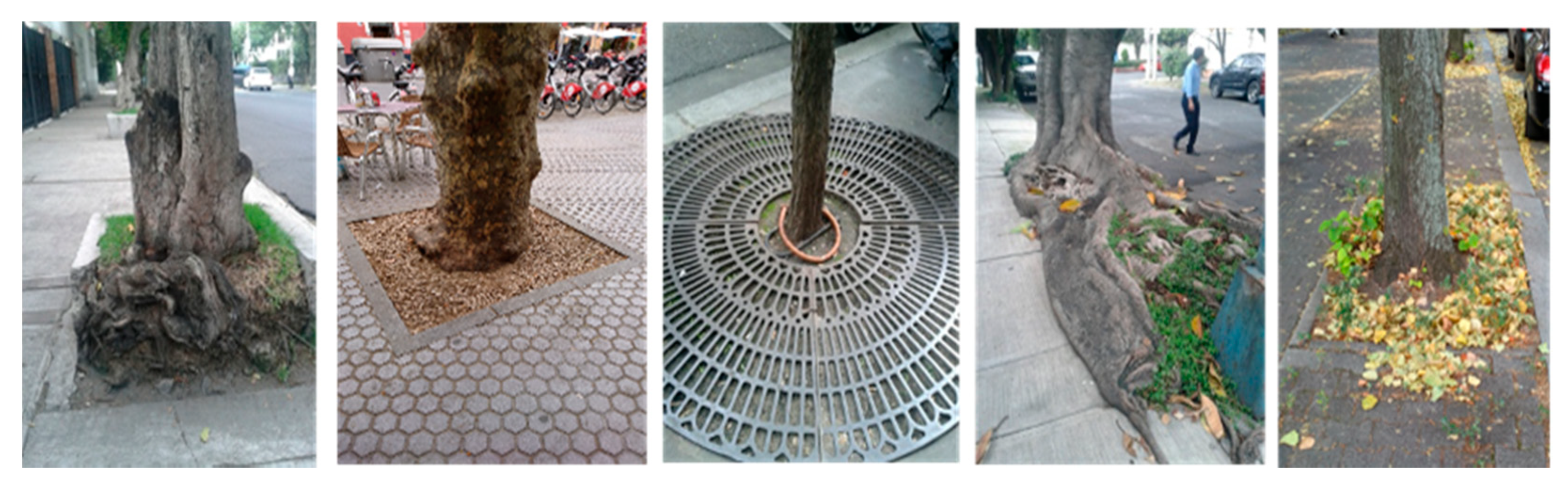
Providing an adequate water supply contributes to more vitality, better growth conditions, and higher ecosystem benefits [16]. In contrast, urban tree growth and ecosystem services may be negatively impacted by soil compaction and/or by paving in combination with summer droughts caused by climate change (Figure 1), with the consequence of limited access to water [1,17,18].

Effects of unusually high temperatures and prolonged dry periods occurred in the last three years (2018, 2019, and 2020), not only in Berlin but also in many other European regions. As a reaction to these extremely dry years, trees showed yellow/brown foliage and/or bare branches in the early summer months. This botanic reaction is common in late autumn. As a result, severe damage to the entire Berlin tree population occurred, indicated by massive deadwood development, fundamental deterioration in vitality, and individual tree mortality [19]. In both years, 2018 and 2019, the State of Berlin spent an additional 2.3 million euros for irrigation measures of city trees [20].

The Department of Economic and Social Affairs Population Dynamics of the United Nations expects that in the next 30 years, about 70% of the world’s population will live in cities [21]. Especially in cities of arid and semi-arid regions, street trees are important for cooling the air temperature by transpiration and shading. They are essential for the quality of life. Thus, it became an essential issue to develop new strategies for greening inner-city places and planting new trees.

2. Materials and Methods

Chapter 2 explains the basic principles of Hydro-Pedo-Transfer Functions (HPTFs) and defines the specific site information, such as climate (rainfall and potential evapotranspiration), soil (water retention and groundwater depth), and tree (species, age, rooting depth, and catchment area), to solve the equations. Examples of how to gain these data either by mapping, measuring, or by using available digital data from various climate panels and soil information systems are also given.

2.1. Principles of Hydro-Pedo-Transfer Functions (HPTFs)

The principal idea behind HPTFs for predicting potential and actual evapotranspiration and groundwater recharge for cropland, grassland, and forest stands is described in detail in [22]. However, for deriving HPTFs for urban street trees, the inner-city growing conditions have to be considered. Therefore, firstly explanations are given of how the HPTFs were derived in principle, followed by modifications for urban site conditions. The procedure for deriving HPTFs contains two steps: First, a conventional soil–vegetation–atmosphere–transpiration model (SVAT) was used to calculate the daily rates of evapotranspiration and percolation [22], using the following input parameters:

• Daily climate data—precipitation, wind velocity, mean air temperature, mean air humidity, and net radiation;
• Soil hydraulic functions—soil water retention, unsaturated hydraulic conductivity, and depth to the groundwater table;
• Plant data—degree of soil cover, rooting depth, plant height, and stomata resistance for various soil moisture conditions.

Actual evapotranspiration (ETI_a) was calculated using the Penman–Monteith approach as modified by Rijtema [23]. Soil hydraulic functions were determined in the laboratory using the instantaneous profile method according to Plagge [24]. Model calibrations use either ETI_a measurements from field studies, lysimeter measurements, or balances of total runoff from catchments [22]. The SVAT model was used for simulations of various combinations of site-specific conditions:

• Four soil textures with plant available water from low to high;
• Deciduous trees;
• Six groundwater table depths (from 0.9 m to 2.8 m deep);
• Sixteen climate stations in Germany.

Secondly, annual actual ETI_a results of >12,000 SVAT simulations for varying water supply conditions were evaluated by means of nonlinear multiple regression analysis using the SPSS software package. Each annual actual ETI_a value was nonlinearly correlated to the following:

• Potential FAO grass reference evapotranspiration (=without any water limitation, ET0) according to Allen et al. [25];
• Site-specific annual water supply (S_w).

The annual water supply (S_w) is defined by the available water resources that plants can use for transpiring, such as summer precipitation (P_s), soil available water in the root zone (W_a), capillary rise from the groundwater to the root zone (Q_a), and runoff (R_o) from surrounding sealed areas, which can be either a gain or a loss:

S_w = P_s + W_a + Q_a ± R_o

(1)

where S_w is the available water supply of the tree catchment area (mm), P_s is the summer precipitation from April 1 to September 30 (mm), W_a is the available soil water in the effective root zone (mm), Q_a is the actual capillary rise from the groundwater (mm), and R_o is the surface runoff (mm), which is either a gain (+) or a loss (−) for the tree depending on the slope and draining direction in the catchment area.

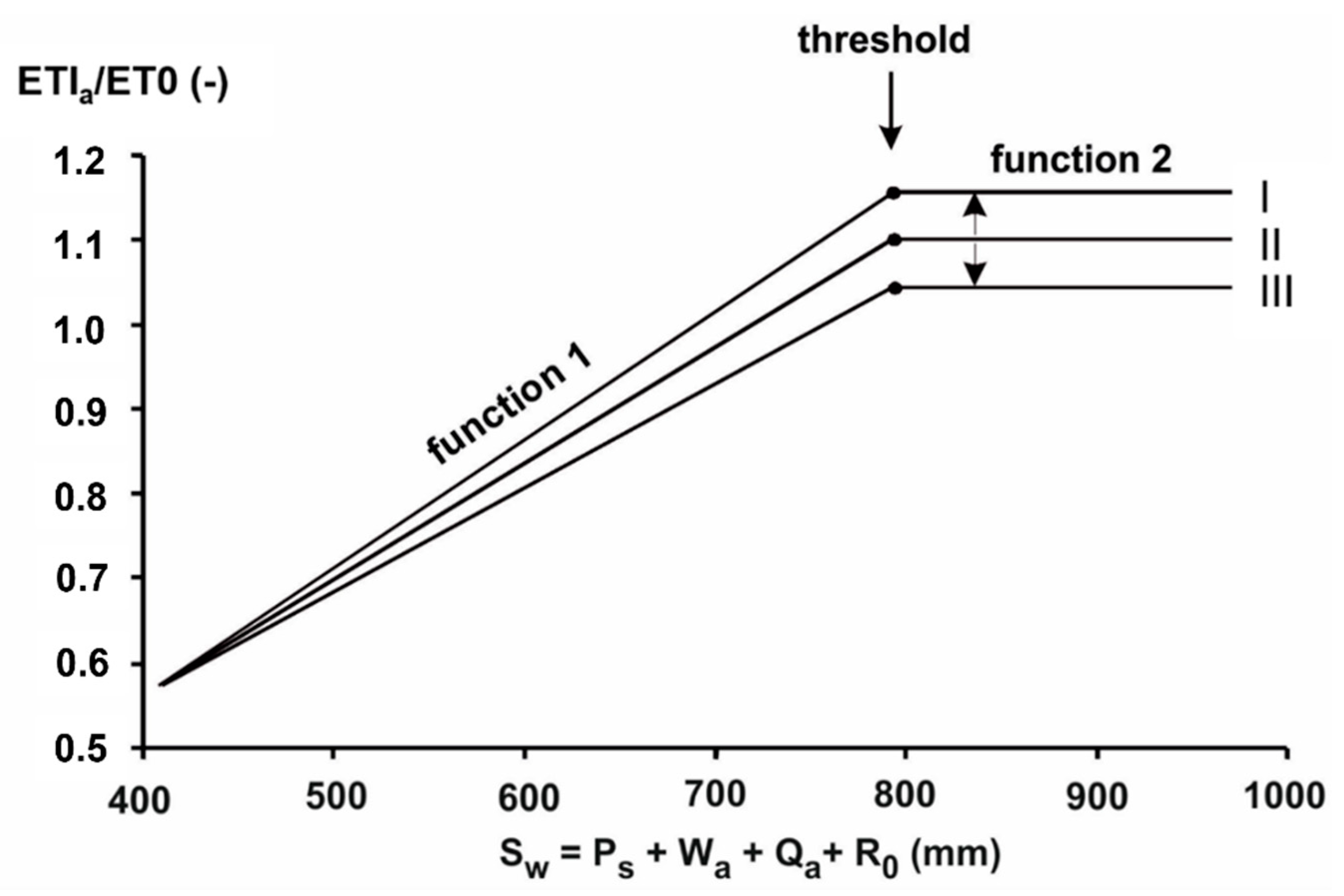
Next, it became necessary to combine both the water supply and the actual evapotranspiration within a logic framework. Figure 2 illustrates the principal idea of the HPTFs describing water stress and water supply: using the ratio of actual evapotranspiration and potential evapotranspiration (ETIa/ET0) against the actual water supply (S_w). Up to a critical threshold (in this case 800 mm), the ratio increases as a function of the water supply using Function 1; above this threshold the ratio only depends on the height of ET0 and can be described by Function 2, which is independent of the amount of Sw. The three lines (I, II, and III) of both functions indicate various levels of ET0.

This HTPF concept, which is often called the “TUB-BGR” approach, introduced and described in detail in Wessolek et al. [22], allows predicting the annual actual evapotranspiration, water stress, and percolation rate for different land usage, climate, and side conditions.

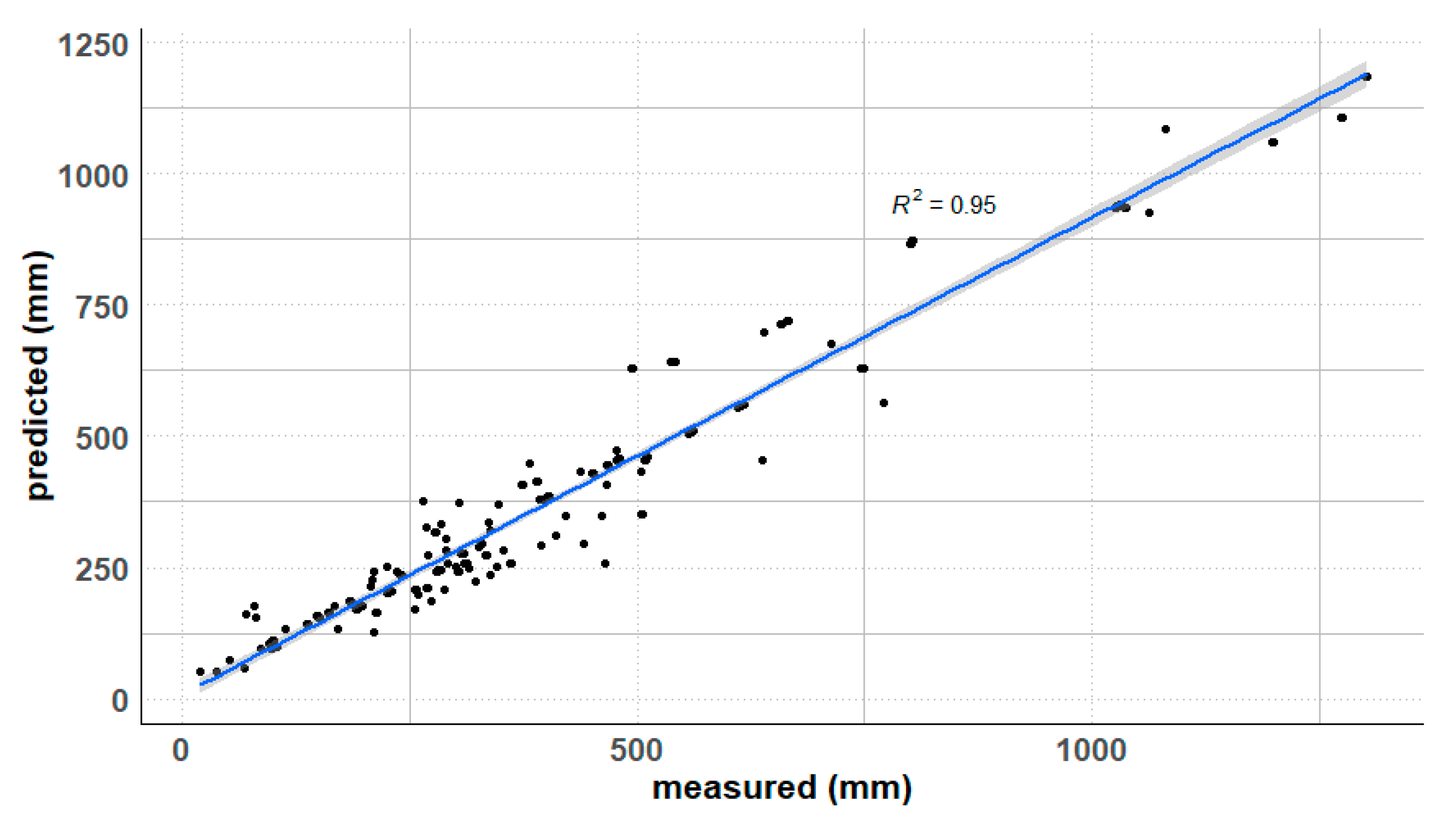
Among others, it has been used to predict the long-term means of the water budget within the framework of the Hydrological Atlas of Germany [26]. The HPTF results have been successfully validated by comparisons with the gauge-measured values of the mean percolation rate (R) + runoff (R_o) taken in 106 different catchment areas in Germany, as shown in Figure 3.

Recently, the HPTF approach also has been successfully tested for water budget predictions and regionalization of drought stress within a German National Forest Inventory [27].

2.2. Conceptual Approach and Deriving Input Parameters

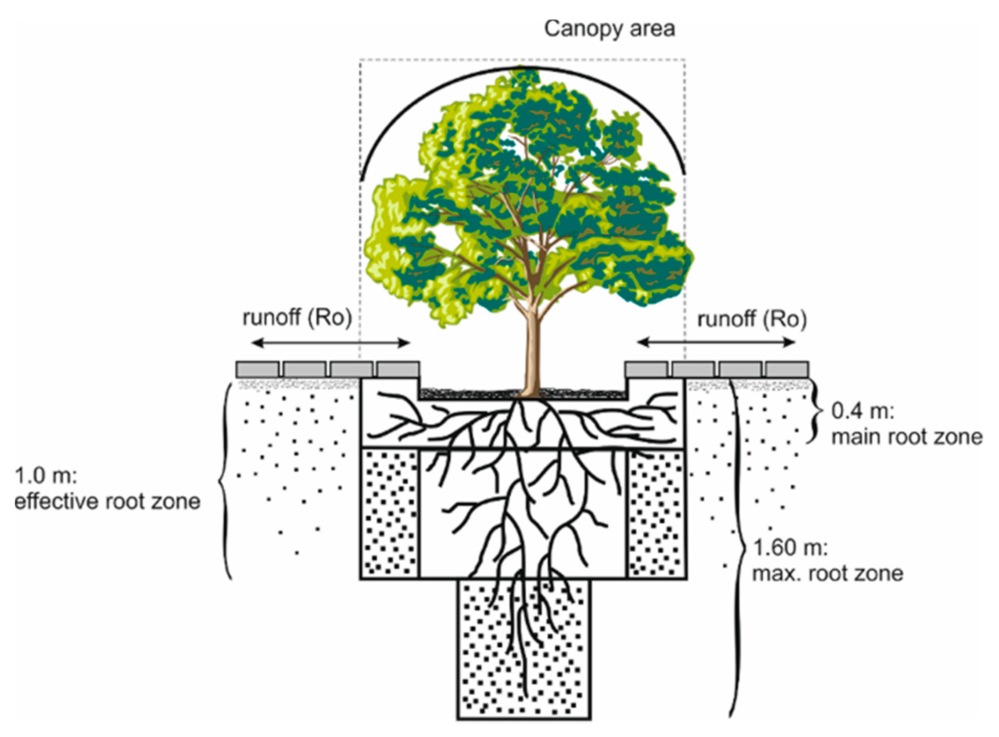
In this chapter, explanations are given of how the HPTF concept has been modified for urban street-tree conditions, and how evapotranspiration and water supply can be calculated easily. In detail, it is demonstrated how environmental factors, such as exposition, location and street type, tree species, soil properties, sealing degree, and climate, are considered. Moreover, information is given on how the input parameters can be derived easily by mapping or by using digital information platforms. Figure 4 shows principally, how street-tree sites can be characterized by (i) the tree canopy, which also defines the catchment area; (ii) soil and surface conditions; and (iii) effective rooting depth.

The tree-canopy radius depends on the tree age and species. In our contribution, we assume that it describes on the ground 1:1 the catchment area beneath the tree crown. If, for example, the canopy has a radius (r) = 3 m, the catchment area (CA), in which root water uptake for evapotranspiration takes place, can be calculated as

CA = π × r²

(2)

where CA is the catchment area (m²) and r the radius of the crown area (m); for example, CA = 3.14 × 9 = 28.26 m².

Rooting depth: In our example, a maximum root depth of 1.6 m, a main root zone of 0.4 m, and a resulting effective root zone of 1.0 m ((1.6 + 0.4)/2) were considered (Figure 4). Runoff from pavement flows either to the tree, thus improving water supply, or leaves the catchment and discharges into the rainwater canalization. Besides the radius of the canopy, one also should take the tree species into account, because tree species behave differently with respect to plant water uptake and transpiration. To describe the relative water demand of the different street-tree species, we suggest using the relative tree water demand coefficients (T_r), as listed in

Table 1. Relative tree water demand (T_r). Examples for various tree species according to Duthweiler et al. [28], Gillner [29], Rahman et al. [16], and Roloff et al. [30].

Tree Species	Tr (-)	Classification
Platanaceae	1.2	high
Tiliaceae	1.2	high
Fagaceae	1.1	medium
Ostrya	1.1	medium
Robinia	0.9	low
Quercus	0.9	low
Castanea	0.8	very low
Betula	0.8	very low

. They describe the relative differences among tree species in terms of their water stress behavior and water demand, as described in literature such as Duthweiler et al. [28], Gillner [29], Rahman et al. [16], and Roloff et al. [30].

However, we set in our calculations T_r = 1.2, according to the original version of the HPTFs developed for deciduous trees, which has been calibrated for stands in Berlin and Hannover, Germany, as described by Wessolek et al. [22]. To simplify the tree root system, the so-called “effective root zone concept” was used, which is introduced and described in detail by Renger and Strebel [31] and Wessolek [32]. These assumptions also rely on German recommendations of the framework ATV-DVWK [33] for predicting evapotranspiration and water components for various land-use systems. All the necessary parameters used in this HPTF approach and relevant sources are listed in

Table 2. Site information needed for predicting water supply and actual evapotranspiration of street trees by HPTFs.

Site Information	Usage for	Sources
Climate
Annual precipitation (mm)	Water balance	Regional or national climate observation stations and services
Summer precipitation (mm) from April 1 to September 30	Water supply (Sw) Actual evapotranspiration (ETIa) Runoff (Ro)
Annual potential evapotranspiration (ET0) according to FAO	Water demand of the atmosphere
Street Tree
Tree species	Water demand	Mapping or digital information of environmental agencies
Radius of the canopy	Catchment area (CA) Water supply (Sw) Actual evapotranspiration (ETIa)
Effective rooting depth	Water in the rooted zone Water supply (Sw) Actual evapotranspiration	Young trees: 0.6 m Medium old trees: 1.0 m Old trees: 1.2 m
Site Characteristics	ET0u, A, and SVF coefficients	Mapping sky view factors
Soil, surface, and groundwater depth
Soil texture	Soil available water in the root zone (Wa)	Mapping or information of the national soil survey
Groundwater depth	Capillary rise (Qa)	Soil survey or environmental agency data
Tree pit conditions	Runoff (Ro), ß coefficients ETIa of grass or sealing beneath the crone	Mapping or information of the local environmental agencies

. Most of the required information, such as precipitation, soil texture, and groundwater depth, are available from national climate service centers or from local or national soil surveys. Tree-specific information, such as age, canopy, plant species, and soil surface (degree of sealing), should be mapped or are, like in Berlin, digitally available from the environmental agency [34].

2.3. Potential Evapotranspiration of Urban Sites (ET0u)

Local site conditions of street trees severely influence the incoming net radiation, wind speed, and air humidity, and thus the microclimate; i.e., the potential evapotranspiration varies to great extent. ET0 can be much lower by the shading effects of buildings or higher by advection processes, resulting in additional energy by lateral heat flow from the surrounding sealed and heated areas. Thus, HPTFs should consider these urban conditions.

Street size, i.e., width, and even more the height of the surrounding buildings influences the incoming light and shading conditions of street trees. As solar radiation [35], especially short-wave radiation [36], is considered the most important factor influencing evapotranspiration, the ET0 values can be smaller or in some cases even higher compared to open, non-urban landscapes.

To design a flexible tool, we followed the landscape coefficient method (LCM) by Costello et al. [37], which includes the so-called microclimate coefficients for adapting the ET0 reference evapotranspiration [25] to specific urban site conditions. The coefficients range between 0.5 and 1.4 depending on the location, e.g., shading degree, strong winds, and lateral energy input [37,38]. Technically, we suggest using the so-called sky view factors (SVF) for taking differences in the degree of shading and radiation into account. SVF describe the ratio between the actual amount of radiation to the potential atmospheric radiation without urban limitations. It is a dimensionless value varying from 0 to 1 [39] and often determined by fish-eye photographs at a pedestrian level. For example, a SVF value of 1 means that the sky is completely visible, as in open and flat landscapes. In street canyons, only part of the sky is visible, which means that radiation is reduced, leading to a coefficient <1. Thus, we define an urban-specific potential evapotranspiration (ET0_u) for sites with a reduced radiation by

ET0_u = SVF × ET0

(3)

where ET0_u is the urban-specific potential evapotranspiration, SVF is the sky view factor, and ET0 is the potential FAO grass reference evapotranspiration according to Allen et al. [25]. The SVF coefficients for various urban site conditions, considering less radiation, are listed in

Table 3. Combination of the SVF coefficients according to Gong et al. [35] and Costello et al. [37], and advection coefficients (A) according to Bohne [40] and Schwärzel and Bohl [41] for various urban sites.

Urban Location	Space, Street Width (m)	Height of Buildings (m)	Degree of Shading **	SVF * (-)	Advection A *** (-)
Street type I	8–15	>15	High	0.4-0.5	-
Street type II	15–20	8–10	Medium	0.7	-
Street type III	20–25	6–8	Low	0.8-1.0	-
Inner-city parks	>25	-	-	1.0	1.2–1.4
Inner-city places with single trees	>25	Additional energy by advection and wind		1.0	1.4–1.6

* For streets with a reduced radiation: ET0_u = SVF × ET0; ** Degree of shading by buildings; *** For sites with an increased energy input by advection: ET0_u = A × ET0.

.

The individual sky view factor for the environment, respectively, the tree surroundings, could be determined for example by free GIS software, such as QGIS [42] and UMEP [43], or RayMan via fish-eye photographs [44].

On the other hand, ET0 might principally increase for inner-city places by advection, i.e., lateral energy flow from surrounding heated areas. In this case, the ET0 should be adapted by using advection coefficients (A) describing the increase in ET0 compared to sites without advection:

ET0_u = A × ET0

(4)

where A is the advection factor and ET0 is the potential FAO grass reference evapotranspiration according to Allen et al. [25].

The A coefficients listed in Table 3 were gained by (i) lysimeter measurements of Bohne [40] and Schwärzel and Bohl [41]; and (ii) by a sensitivity study on the influence of increasing temperatures and radiation on potential evapotranspiration, done by Wessolek [45]. Using these SVF and A coefficients is the first integrated and practicable attempt considering the influence of urban conditions on ET0 predictions. The influence of various ET0 levels is included in Figure 2. It shows how the ratio of ETI_a/ET0 reacts on various ET0 levels (Type I: A = 1.0; Type II: A = 1.2; and Type III: A = 1.3). In this example, Type II and Type III indicate additional energy by advection from the environment.

2.4. Soil Available Soil Water in the Effective Root Zone (W_a)

Soil physical field and lab measurements can be used for the estimation of the soil available soil water (W_a) in the effective root zone, in which S_aw describes the soil available water held between the water tension at field capacity (pF 1.8) and permanent wilting point (pF 4.2), according to Renger et al. [46]. If these data are not available, the so-called Pedo-Transfer Functions (PTFs) can be easily applied to predict soil water retention by the methods suggested by Vereecken et al. [47] and Wösten et al. [48]; those in Zacharias and Wessolek [49] are also suitable and available. In addition, soil physical data of the national soil survey service can be used easily. The soil available water (W_a) in the effective root zone (W_e) of trees can be predicted by

W_a = S_aw × W_e

(5)

where W_a is the soil available soil water in the effective root zone (mm), S_aw is the soil available water between the water tension pF 1.8–4.2, and W_e is the effective root zone (m).

Table 4. Mean effective root depths (m) of the street trees, adapted from Wessolek in ATV-DVWK [33].

Tree Age Soil Conditions	Young Trees (<15 Years)	Middle Aged Trees (15–30 Years)	Old Trees (>30 Years)
Urban soils without severe compaction allowing deep rooting	0.3–1.0	1.0–2.0	2.0–2.5
Compacted soils or stony soils allowing shallow rooting only	0.3–0.7 *	0.7–1.2 *	>1.2 *

* = Maximum depth (m) until a stone layer, concrete, or compacted soil horizons occurs.

shows exemplarily the mean effective root depths of the differently aged trees and soil materials, and

Table 5. Examples of soil available water in the effective root zone, W_a (mm), for different soil texture classes and dry bulk densities (B_d) **, according to Renger et al. [46].

Soil Criteria		Bulk Density (Bd) **
		Bd ** (g/cm3)	1.3–1.5			>1.5 (g/cm3)
Texture class	Soil available water * (Saw) (vol.%)	Effective root depth, We (m)	0.8	1.0	1.2	0.8	1.0	1.2
	Range	Tree age (years)	<15	15–30	>30	<15	15–30	>30
Medium sandy soil	8–12	Soil available water in the effective root zone (Wa) (mm)	80	100	120	75	95	115
Fine sandy soil	12–15		120	150	180	110	140	170
Loamy sand	12–16		128	160	192	112	140	168
Sandy loam	13–17		136	170	204	116	150	174
Silty soil	20–24		176	220	244	160	200	240
Clayey soil	7–12		96	120	144	56	70	84

* S_aw: moisture between the pressure head pF 1.8–pF 4.2 (vol.%); ** B_d: bulk density (g cm⁻³).

gives a first orientation of the mean soil available water of the various soil substrates while the range of soil available water (S_aw) varies soil dependently from 8 to 20 vol.%. Thus, the mean available water varies between 80 for young tree and 120 mm for an old tree growing in sandy substrates and could reach a span from 160 mm until 240 mm per square meters for trees growing on silty soils, respectively.

Using this information, the total amount of available water (in liter) within the catchment area (C_wa) can be calculated by

C_wa = W_a + P_s × A (mm)

(6)

where C_wa is the total amount of available water within the tree catchment area, W_a is the soil available water in the effective root zone (mm), P_S is the summer precipitation from 1 April to 30 September (mm), and A is the catchment area (m²).

Example:

A 15-year-old street tree having (i) a catchment area of 28 m²; (ii) an effective root zone of W_e = 1.0 m; and (iii) is growing in Berlin in a medium compacted sandy soil with an S_aw = 9 vol.%. The site is groundwater distant, i.e., no capillary rise occurs. The mean summer precipitation in Berlin is P_s = 300 mm, and no runoff occurs. In this case, one gets W_a = 9 ×10 (dm) = 90 L/m².

Thus, C_wa= (90 + 300) × 28 = 10,920 L soil available water in the effective root zone can be expected for the total tree catchment. Assuming a mean actual evapotranspiration per day and square meter catchment of 3 mm per day, the total tree water uptake out of the catchment is 28 × 3 = 84 L. In Germany, the mean active vegetation period is about 120 days per year (Mai, 1 till September 30th). Thus, a tree transpires in total 120 × 84 = 10,080 L. In this example, one can conclude that soil water storage of the catchment is sufficient for supporting the tree with water during the vegetation period.

2.5. Predicting Actual Capillary Rise (Q_a) from the Groundwater

The actual average capillary rise from the groundwater (Q_a) is not only dependent on the soil hydraulic functions but is additionally affected by climate. Thus, both a soil- and climate-specific limitation of capillary rise has to be considered, as is presented now.

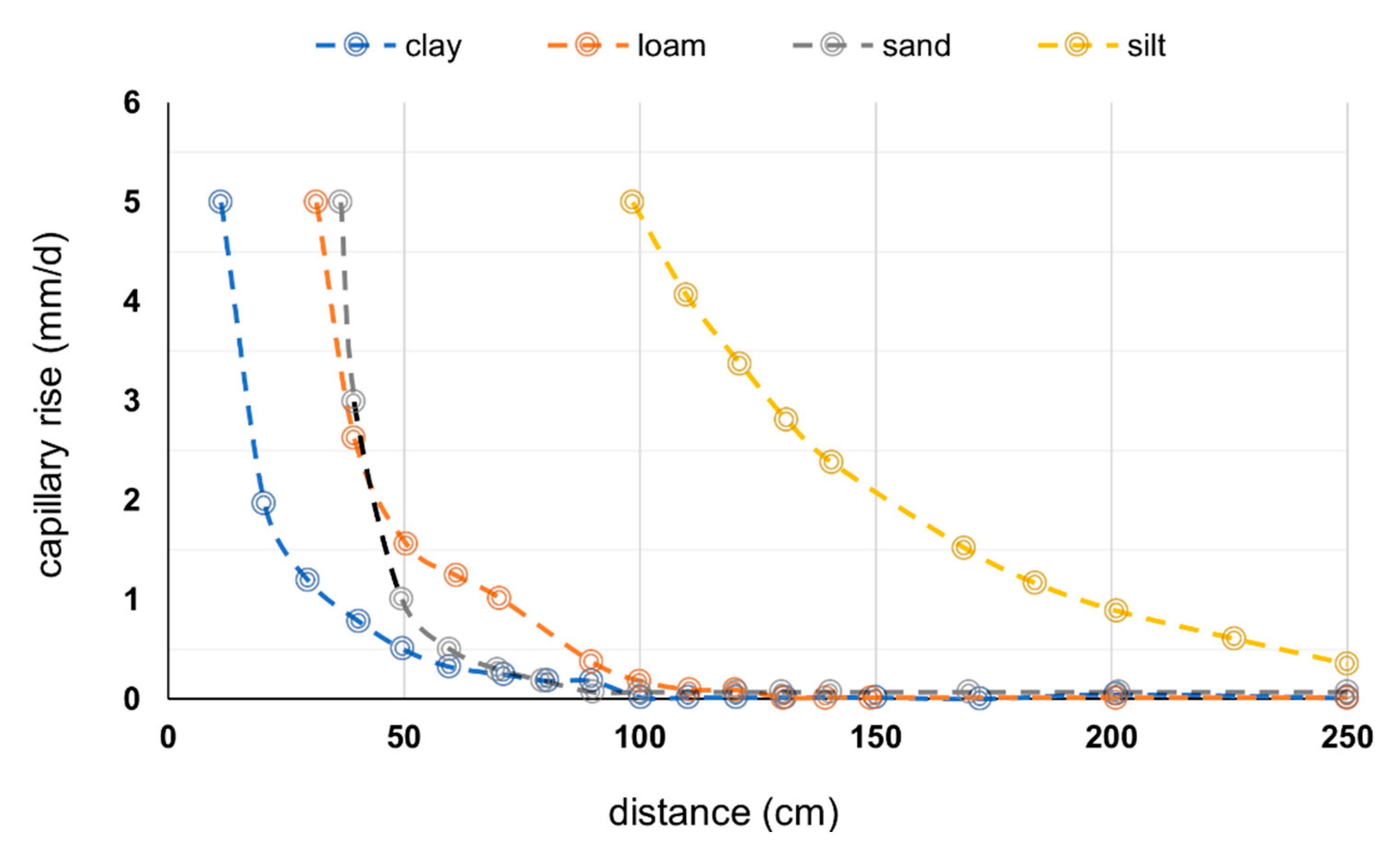
First, the soil-specific capillary rise must be calculated. For this, steady-state capillary flow rates can be used, as listed for all soil textures in the German Soil Classification System KA5 [50]. They are called “potential capillary rise rates” (Q_pot) because they express the daily potential upward flow rates without climatic limitation. They have been calculated by solving the Darcy equation numerically for various steady-state pressure heads and distances between the groundwater table and the bottom of the effective root zone. Figure 5 shows the potential capillary rise rates (Q_pot) for the typical soil textures, according to the German Soil Classification System KA5 [51].

Next, the tree-specific time (T in days) in which an active uptake of capillary rise takes place must be considered. In Germany, this active period of water uptake corresponds with the active vegetation period and starts in May and ends in September (120 d). Detailed information can be taken from the Ad-Hoc AG Boden [51]. Hence, the maximum annual capillary rise of the groundwater (Q_max) to the root zone is given by

Q_max = Q_pot × T

(7)

where Q_max is the maximum annual capillary rise of the groundwater (mm/d), Q_pot is potential capillary rise rate (mm/d), and T is the time (d).

In the next step, the upper limit of capillary rise depending solely on climatic conditions must be estimated. We call this the “climate controlled annual capillary rise” (Q_cli), which can be calculated by using the following equation considering site and climate specific factors according to Wessolek et al. [22]:

Q_cli = 1.3 × E_o,s − (P_s + 0.5 × W_a)

(8)

where Q_cli is the climate- and site-controlled annual capillary rise (mm), E_o,s is the potential FAO grass reference evapotranspiration in the summer time from April till September (mm), P_s is the sum of the summer precipitation from April till September (mm), and W_a is the soil available water in the root zone (mm).

The empirical coefficient 1.3 in Equation (8) expresses methodical differences in the calculation of the potential evapotranspiration (ET0) according to the FAO [25] and a modified Penman-Monteith-approach, which was used in the derivation of the HPTF [22]. The coefficient 0.5 multiplied with W_a (Equation (8)) results from field observations and measurements made on various locations influenced by groundwater, where it was observed that the process of capillary rise into the root zone started when 50% soil available water or less was reached [31].

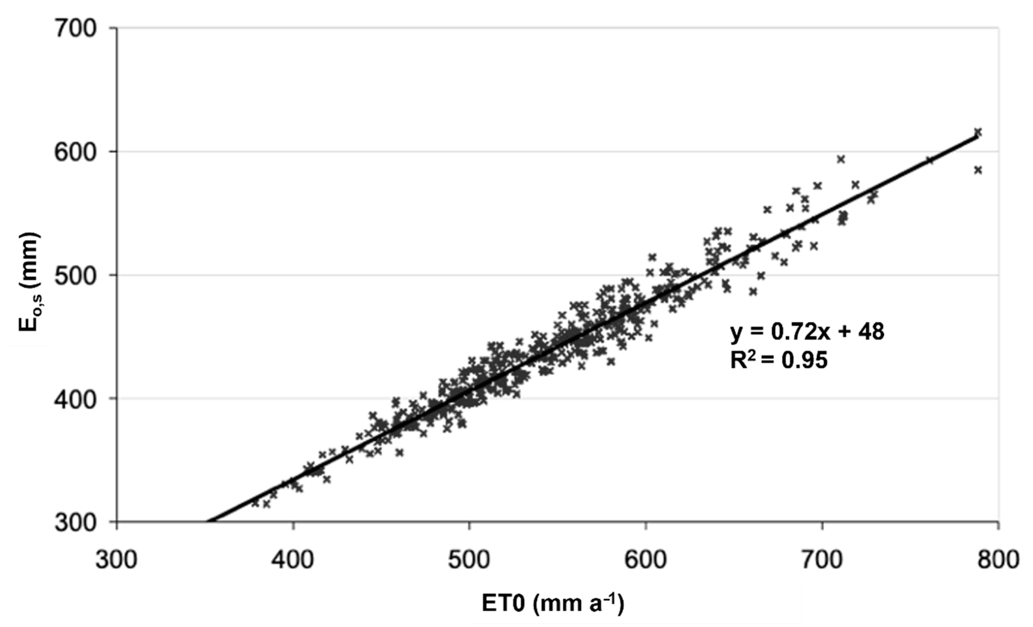
E_o,s in Equation (8) can be calculated by a simple linear regression equation relating the FAO grass reference evapotranspiration of the summer half-year (from April until September, E_O,S) to the ET0 of the entire year, as shown in Equation (9). This relation has been predicted for various locations in Germany for the period between 1961 and 1990 [22]. A linear regression analysis between ET0 and E_o,s shows a close relation (Figure 6). The equation for the German climate conditions is

E_o,s = 0.7158 × ET0 + 48

(9)

where E_o,s is the potential FAO grass reference evapotranspiration in the summer time (April–September (mm), and ET0 is the annual potential FAO grass reference evapotranspiration according to Allen et al. [25].

To make a realistic assessment of the actual amount of annual capillary rise (Q_a) needed for the HPTF, three conditions for Q_a may be distinguished [22]:

if Q_cli < 0, then Q_a = 0
if Q_max > Qcli, then Q_a = Q_cli
if Q_max ≤ Q_cli, then Q_a = Q_max

(10)

where Q_a is the actual amount of annual capillary rise, Q_cli is the climate- and site-controlled annual capillary rise (mm), and Q_max is the maximum annual capillary rise of groundwater (mm/d).

2.6. Estimating Runoff (R_o)

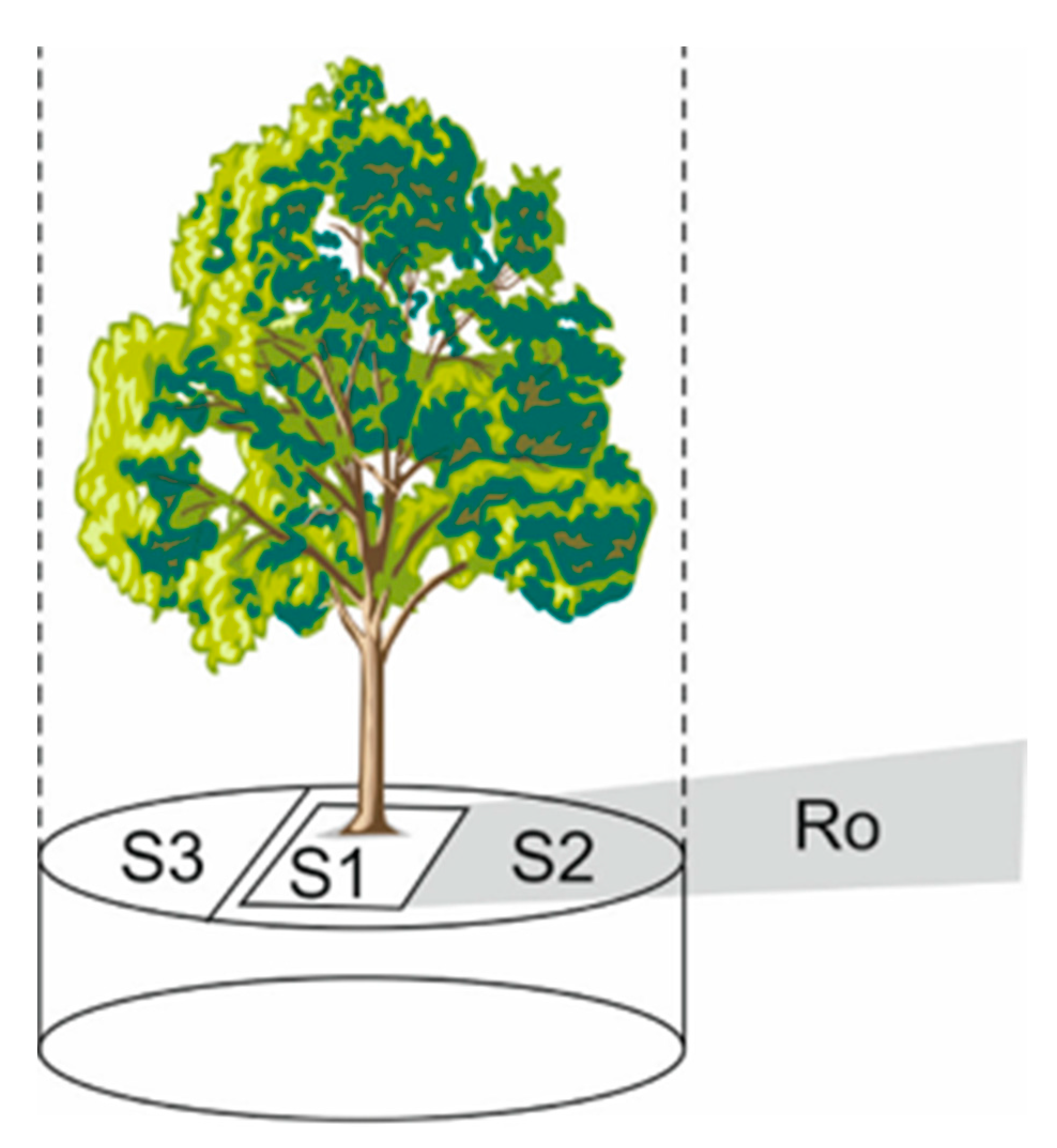
Runoff (R_o) depends on the slope and structure of the soil surface in and besides the tree catchment. If, for example, the areas S1, S2, and S3 (see Figure 7) beneath the canopy are located deeper than the surrounding areas, runoff from outside might enter the catchment area, leading to an increase in S_W. However, if S1, S2, and S3 are in a higher position compared to the surrounding level, then runoff might leave the catchment. This situation can be observed when older street trees do not have enough space for rooting and growing, leading to an upwards lift of the tree stump compared to the surrounding surface level.

Lysimeter studies and infiltration measurements of various urban areas show that Ro varies to a great extent, depending on the percentage of gaps among the pavement materials, rainfall intensity, and the age of the pavement. During the aging of the pavement, dust input reduces the infiltration and thus increases runoff [50,52,53,54].

For predicting annual values, we suggest using β-infiltration coefficients, as listed in

Table 6. ß-coefficients for summer (s) and winter (w) for the different sealing classes (I–IV), with examples according to the site and lysimeter studies of Wessolek et al. [22,53].

Degree of Surface Sealing	βs	ßw	Pavement Type
Class I (low: <10%)	0.90	0.95	unsealed soil, concrete stones with grass
Class II (med.: 10–50%)	0.80	0.85	small cobblestones
Class III (high: 90–50%)	0.55	0.60	concrete pavement
Class IV (severe: >90%)	0.20	0.25	asphalt
Class I	Class II	Class III	Class IV

. They express both (i) the runoff (R_o) leaving the sealed surface; and (ii) the amount of rainfall that infiltrates either through gaps of the seam material or directly into the surrounding soil. Because of higher rainfall intensities in summer, we suggest distinguishing between the ß-coefficients for summer (P_s) and winter precipitation (P_w), as shown in Table 6. However, for predicting tree water supply, it becomes necessary to consider only the runoff of summer precipitation, because it might increase or decrease the amount of water supply. Thus, for each unit of the canopy area, we calculate

R_o = P_s × ß_s

(11)

where R_o is the runoff that might increase or decrease the water supply of the tree (mm), P_s is the sum of the summer precipitation from April to September (mm), and ß_s = the summer runoff coefficient for various degrees of surface sealing (Table 6).

R_o (mm) is the total amount of runoff during summertime that could either deliver or discharge surface water from or into the catchment area of the tree, as shown in Figure 7. For each catchment unit (S1, n), runoff (R_o) should be predicted by

R_o = [(1 − ß_s) × P_s] × α

(12)

with

R_o = Σ R_o1 ± R_o2 ± R_o3 ± R_o4

(13)

For each segment, R_o is to be calculated by

R_o = α · ß_s · P_s

(14)

where R_o is the total runoff of all catchment units (S_1,n) during summertime (mm), ß_s is the infiltration coefficient for summer rain (-), and α is the share of the sealing unit (%) within the total catchment area, and n is the number of catchment units.

Using the above presented information on P_s, W_a, Q_a, and R_o, water supply (S_w) for the tree per unit catchment area can be predicted. How it is used for calculating the actual evapotranspiration of the street trees is explained in the following section.

2.7. Predicting the Actual Evapotranspiration of Street Trees

For predicting the actual evapotranspiration per unit catchment area, one first has to distinguish between two situations: sites that do not have a sufficient water supply to enable potential evapotranspiration (S_w < 800 mm = Function 1, Figure 2) and those with a sufficient water supply (S_w> 800 mm = Function 2, Figure 2). Thus, two HPTFs were derived by introducing a threshold of the so-called ‘critical water supply’. In Germany, this critical water supply (S_w) equals 700 mm for croplands and grasslands and increases up to 800 mm for forest stands [23].

If the water supply (S_w) is limited, i.e., S_W ≤ 800 mm, then the actual evapotranspiration (ETI_a) for each square meter of the street-tree catchment can be calculated using Function 1:

ETI_a = T_r × ET0_u [1.61 log (S_w) − 3.39] × [0.865 log (1/ET0_u) × 3.36]

(15)

where ETI_a is the actual evapotranspiration (mm/a), T_r = relative tree water demand (-), ET0_u is the potential urban evapotranspiration (mm/a), and S_w is the water supply as explained by Equation (1). A water shortage for trees in the catchment occurs whenever ETI_a < ET0_u. Thus, the ratio of ETI_a/ET0_u can be used to characterize four cases of water deficiency in the catchment:

(i)

ETI_a/ET0_u > 0.8, indicating a good water supply, i.e., no water stress;

(ii)

ETI_a/ET0_u ranges from 0.8 to 0.6, indicating low to medium water stress;

(iii)

ETI_a/ET0_u ranges from 0.6 to 0.4, indicating moderate water-stress conditions;

(iv)

ETI_a/ET0_u < 0.4, indicating high up to severe water stress.

However, if water supply (Sw) is unlimited, i.e., Sw > 800 mm, the ETIa for each square meter street tree catchment can be calculated by using the above Equation (16):

ETI_a = T_r × 1.25 × ET0_u [0.865 log (1/ET0_u) + 3.36]

(16)

Function (16) should be typically used for regions with high summer rainfall and/or sites with a shallow groundwater table. This becomes relevant when the mean groundwater table for sandy soils is <2.0 m below surface, and for silty and loamy soils < 2.5 m. For German climate conditions, the mean precipitation for summer and winter time as well as annual potential evapotranspiration ET0 can be either taken from the Hydrological Atlas of Germany (HAD) or the German weather service (DWD), or has to be calculated as described in Allen et al. [25] and explained in detail using the framework of the ATV-DVWK [33].

2.8. Predicting the Actual Evapotranspiration of Sealed Areas

To compare street trees with sealed urban surroundings, it becomes necessary to predict the actual evaporation of the sealed areas. According to former investigations presented in Wessolek et al. [22], the actual evapotranspiration from sealed areas can be predicted using Equation (17):

E_as = κ × ET0_u

(17)

in which κ is derived by

κ = log [(0.6 × ß_s × Ps)/log (ET0_u,s)]⁴

(18)

where Eas is the actual evapotranspiration of the sealed areas (mm), κ is the reduction coefficient (-), ET0_u is the potential urban evapotranspiration of the entire year (mm), and ET0_u,s is the potential urban evapotranspiration from April to September (mm).

3. Field Investigations and Mapping

To test the concept and to calibrate the actual evapotranspiration predictions, both sap-flow measurements from two Linden trees and street site mappings were done in Berlin from 2017 till 2020. Linden trees were chosen as it is the most frequent street tree in the inner city of Berlin. It is likely to be tolerant of shade and drought [55,56]. Additionally, the sap-flow results published by Rahman et al. [57] were used for this study.

3.1. Sap-Flow Measurements

From the end of April to September 2018 and 2019, the sap-flux density was measured per unit conducted sap-flow area (J_S) using heat dissipation probes from UP GmbH, according to Granier [58]. One pair of sap-flow probes were installed at 1.3 m height at the north side of each tree to avoid heat stress. The heated probe was installed 10 cm above the unheated to avoid thermal interferences. To provide waterproofing and thermal insulation and direct solar radiation, the sensors’ needles were covered with a terostat and reflective radiation shields. SF measurements were taken every minute, averaged as 5 min data and stored in a GP2 datalogger (Delta-T devices).

Temperature differences were converted to sap-flow densities (J_S) in mL H₂O cm²/min following Granier’s equation [58]:

Js = 0.714 [(∆T_M − ∆T/∆T)]^1.231

(19)

where ∆T_M (°C) is the maximum nighttime temperature difference between the heated and unheated sensors, and ∆T is the mean temperature difference between sensors during each half-hour measurement interval.

We followed the original Granier’s approach [58] and determined ΔT_M on a 24 h basis to calculate the daily Js.

Sap-flow densities were converted to sap-flow by multiplying Js with the sapwood area (cm²), examined by the diameter of the tree at 1.3 m height at different years.

SF = Js × SA

(20)

where SF is the sap flow (mL tree/min), Js is the sap-flow density (mL cm²/min), and SA is the sap-flow area (cm²).

3.2. Tree and Site Conditions

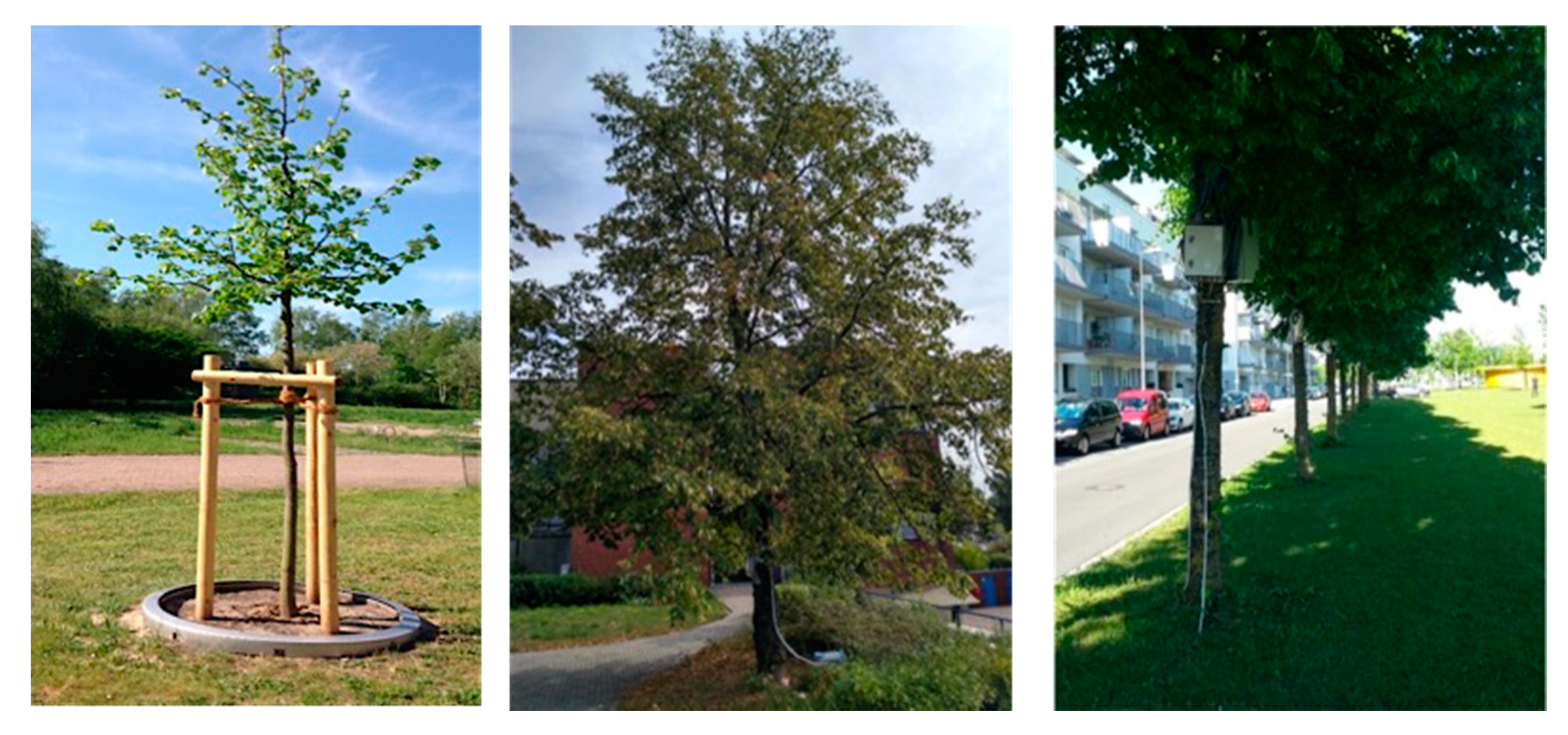
Figure 8 shows the three trees used for the sap-flow measurements and their individual site, i.e., individual growing conditions. The sap-flow measurements of a young Linden tree were done in 2019 and 2020 at the experimental station of the UBA in Berlin-Marienfelde. The tree was about 10 years old, and was planted in a steel lysimeter in 2017, which was filled with a medium sand. The tree is growing as a single tree surrounded by an open space with sparsely vegetation, thus yielding in additional lateral energy input (advection).

Not far away from this site, a 45-year-old Linden tree was used for sap-flow studies in 2019 and 2020 in a park-like environment. This tree is also growing in sandy soil. The tree pit beneath the crone is partly covered with grass vegetation and bushes. The catchment area beneath the crown is about 26 m². In addition, the sap-flow results of a 35-year-old Linden tree gained in 2017 by Rahman et al. [57] in Munich were used for this study. The tree is growing in silty sand besides a road. The tree pit is covered with lawn. Data of this tree were used to recalculate the actual evapotranspiration and water supply in 2017. However, as Figure 8 (right) shows, it is possible that the sensors were not completely shielded against sunlight.

3.3. Climate Conditions

The climate data of Berlin, such as the rainfall, temperature, air humidity, radiation, and wind speed, were measured for Site Nos. 1 and 2 at the experimental station of the UBA, while climate data for Munich were taken from the German weather service (DWD).

Because most experiments as well as the street site mapping were done in Berlin, a short climate characterization should be given.

The city of Berlin lies in a temperate transitional zone between maritime and continental climates, with a 9.1 °C long-term average temperature. In the summer, the mean maximum air temperature is 26.6 °C. January is the coldest month, with a mean air temperature of 2.1 °C.

Annual precipitation fluctuates around 510–650 mm, and the long-term mean is about 587 mm [59], of which 327 mm falls during the vegetation period (April till September). The mean FAO potential grass reference evapotranspiration (ET0) is about 625 mm.

3.4. Street-Tree Mapping

Streets trees have been mapped and analyzed with the assistance of master students studying ‘Urban Ecosystem Science’ at the Technische Universität Berlin. In total, five inner-city streets of Berlin (52°31′ N, 13°24′ E) were mapped and classified uniformly according to the criteria in Table 2. Results of the Kufsteiner Street are presented in this paper, because the tree age varies from <10 years up to >40 years, and the trees are characterized by diverse growing types, heights, and canopy diameters [60].

4. Results and Discussion

4.1. Sap-Flow Measurements and Actual Evapotranspiration

Results of the sap-flow measurements and HPTF predictions for the three Linden trees of Sites I, II, and III are presented in

Table 7. Site conditions, and the measured and predicted evapotranspiration.

Years of Investigation City Site No.	2019 to 2020 Berlin I		2019 to 2020 Berlin II		2017 Munich III
Tree species, age	Tilia cordata, young tree, about 10a		Tilia cordata, middle aged tree, 30–40a		Tilia cordata, middle aged tree, 35a
Measurements	Sap flow		Sap flow		Sap flow Rahman et al. [57]
Site, i.e., street condition	Experimental area: single tree oasis effect		Park similar site		Street width: 25m; building height: 7m
Tree pit condition	Bare soil		Grass		Lawn
Year	2019	2020	2019	2020	2017
Coefficients (A, SVF) for ET0	1.6	1.6	1.4	1.4	0.75
Summer rainfall, Ps (mm)	104	205	104	205	612
Irrigation (mm)	702	720	-	-	-
Soil available water root zone, Wa (mm) ***	120	120	120	120	100
Rooting depth (dm)	10	11	10	10	10
Relative tree water demand (-)	1.2	1.2	1.2	1.2	1.2
Water supply, Sw (mm)	886	1025	102	398	712
ET0 (mm/a)	774	812	774	812	504
ET0u (mm/a)	1238	1299	1084	1137	378
ET0u,s (April–September) (mm)	1014	983	828	866	320
ETIa predicted (April–September) (mm)	899	960	319	331	421
Ta measured by sap flow (mm) *	780	942	256	251	265
Interception and evaporation of the street pit ** (mm)	50	60	64	62	66
Sum of Ta measured + ETIa of street pit (mm)	830	1022	320	314	331
Δ ETIa = ETIa predicted − ETIa measured (mm)	69	-62	-1	18	90
Deviation (%)	7.6	-6.4	<1	5.4	21.4

* Sap flow from April till September expressing the transpiration of the tree = Ta (mm). ** Because T_a excludes both the interception and evaporation of the tree pit, T was adjusted using factors varying from 1.06 to 1.25, according to ATV-DVWK [34]. *** W_a was predicted from soil textural data using the pedo-transfer functions according to Renger et al. [51].

. The right column lists criteria such as tree age and species, growing conditions, summer rainfall, irrigation, and soil available water in the root zone. Moreover, results of the potential evapotranspiration (ET0) for both vegetation periods and entire years are given. Finally, results of the actual evapotranspiration (ETI_a) gained by both sap-flow measurements and HTPF predictions are presented. There is a number of publications that claim that sap-flow measurements by Granier or others underestimate the actual water consumption of trees, such as Steppe et al. [61] and Fuchs et al. [62]. They conclude that a species-specific calibration is necessary when using any of these techniques to ensure that accurate estimates of sap-flux density are obtained.

Moreover, because sap flow only expresses the active water transport used for transpiration of the tree, it does not contain interception, nor the evapotranspiration losses of the tree pit. Thus, it became necessary to adjust the sap-flow rates by introducing correction factors varying from 1.06 for the young tree to 1.25 for the middle-aged tree, according to the framework of ATV-DVWK [34].

First, we discuss the results of the young Linden tree. Both years (2019 and 2020) were characterized by extremely high temperatures and only limited summer precipitation (104 mm in 2019, and 225 mm in 2020). Thus, extremely high potential evapotranspiration rates occurred in both years. To keep the young Linden tree vital and alive, a high amount of irrigation rates was applied in both years, in total >700 mm.

It was interesting to observe that the measured values of the actual transpiration became higher than the predicted potential evapotranspiration (ET0), which indicates a typical so-called oasis effect, expressing advection processes. This phenomenon occurs when a plant, i.e., a tree without any water deficiency, is growing in a large and dry environment. Thus, the lysimeter measurement allows predicting the so-called enhancement factor (A), expressing the increase in potential evapotranspiration by advection (A × ET0). For the site conditions of the young Linden tree on the experimental station of the UBA, the A factor became 1.6, while for the middle-aged Linden tree not far away from site I, an A factor of 1.4 was derived. However, this tree was growing under more park-like conditions with less lateral energy influence and without irrigation. Because of the high amounts of irrigation (>700 mm), nearly no water stress occurred for the young Linden tree, while the middle-aged tree, without irrigation (site II), transpired half the normal amount and less. In 2019, the predicted ETI_a of the young Linden tree is slightly higher compared to the measured one; in 2020, the opposite happened. However, both are in the same order of magnitude. Looking at the low deviation between the measured and predicted ETI_a values of 6.5%, one can conclude for both tree conditions that the HPTF approach works surprisingly well.

Comparing now the sap-flow measurements of Rahman, who used a middle-aged Linden tree growing in Munich (Site No. III), with the HPTF results, one gets a clear overprediction of ETI_a. One reason could be that the HPTFs underestimate the water consumption of the growing lawn beneath the tree, leading to an overprediction of the ETI_a of the tree.

Another reason could be the fact that Rahman published aggregated data, i.e., mean sap-flow values over three months (May, June, and July), while we calculated the ETI_a for the whole vegetation period. At least, we cannot exclude that the sensor needles were not completely shielded against sunlight, as Figure 8 (right) shows, yielding in an underestimation of the flow rates.

4.2. Street-Tree Mapping

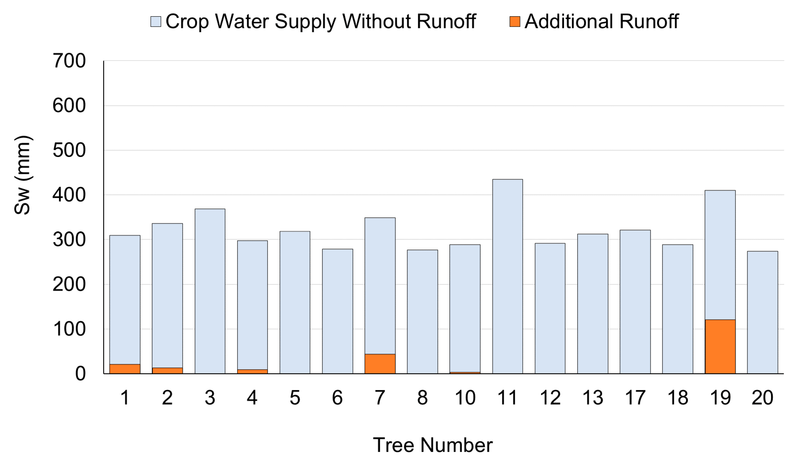
The mapping results and water supply (S_w) predictions of in total 20 trees located at the Kufsteiner Straße are presented and discussed in this section (Figure 9). Tree age varies from a recently planted street tree (No. 11) to a medium old one (No. 2, about 13 years old), up to well-established trees (No. 6 and No. 12) with >30 years.

Thus, tree catchment beneath the crone varies from 5m² for the young tree up to >150 m² for well-established street trees. Hence, one can conclude that individual tree catchment and water supply is not constant but increasing because the tree, i.e., its canopy, is growing. Water supply (S_w) of the 20 tree-catchment areas is exemplarily presented for the Kufsteiner Straße. S_w varies between 280 mm and 430 mm (Figure 9). The highest S_w values were found for the youngest tree, No, 11, because (i) due to the high soil available water of the organic-enriched planting substrate used for the tree; and (ii) no runoff losses occurred on the unsealed catchment. However, when trees become older, three processes happen: first, the rooting system exceeds into the parent sandy soil material, in which the soil available water is lower; secondly, the tree is slightly lifted because the root volume exceeds; and thirdly, the pit, i.e., the ground of the catchment, is more-and-more covered with sealing materials. Thus, runoff occurs, leading to a much lower S_w. Only for a few trees (such as No. 7 and No. 19), S_w is slightly increased by the additional runoff water, coming from the surrounding sealed areas into the catchment of these trees.

Most trees are subject to severe drought, i.e., water deficiency, because their S_w is low. On average, it is only about 35–40% of the critical threshold for S_w, which needs to be approximately 800 mm for a no-water-stress condition.

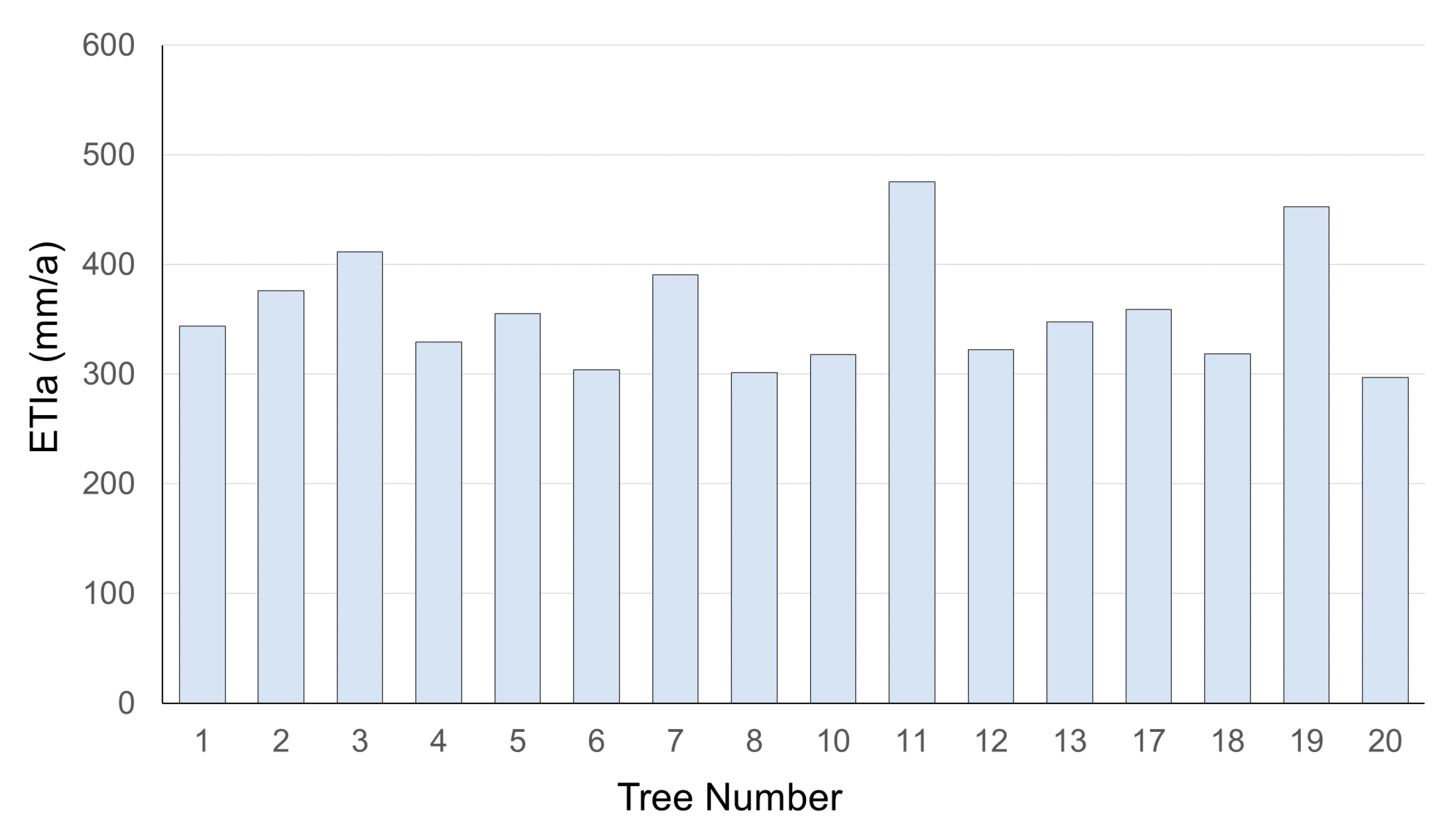
4.3. Case Studies on Evapotranspiration and Water-Stress Predictions (ETI_a/ET0)

Differences in water supply (S_w) between the tree catchments consequently influence the mean annual actual evapotranspiration and water budget, as is shown in Figure 10 for all trees of the Kufsteiner Straße. Thus, the highest annual actual evapotranspiration (mm/a) per square meter catchment has been predicted for young trees, such as No. 11, and lowest for older ones, i.e., well-established trees. Detailed information is listed in

Table 8. Water supply, evapotranspiration, and tree water stress (ETI_a/ET0) of three exemplarily street-tree catchments in the Kufsteiner Straße Berlin, Germany.

Street-Tree No. Age	11 Young	2 Middle	6 and 12 Middle-Old
Mean water supply, Sw (mm) of the catchment	430	320	310
Catchment area (m2)	4.9	45.4	153.9
Cwa of the total catchment to 1m depth (L)	2400	14,500	43,100
Mean annual ET0u (mm/a) for A = 1.0	625	625	625
Mean ET0u (mm/a) during the vegetation period	498	498	498
Mean annual ETIa (mm/a)	480	380	285
Mean ETIa (mm/a) during the vegetation period	394	322	253
Mean ETIa per day (mm/d) during the vegetation period	2.2	1.8	1.4
Water deficiency stress: ETIa/ET0u (-)	0.8	0.6	0.5
Drought rating	‘low’	‘medium’	‘high’
Mean daily water uptake of the catchment (L) (Apr.–Sept.)	11	82	215
Additional runoff into the tree catchment (L)	0	2752	761

and explained by their individual water supply as shown in Figure 9. As mentioned before, the S_w sources are coming either from soil available water (S_aw), summer precipitation (P_s), or additional runoff that can be either a loss or a gain. Thus, S_w varies from 2400 L for the young tree till 43,100 L for the already established trees. This total amount of water is available for the whole catchment area for evapotranspiration, i.e., cooling the atmosphere.

The highest actual evapotranspiration rates can be expected from the catchments with young trees because their tree canopy is still small and no or few runoff losses occur.

Thus, the S_w per unit catchment area is significantly higher for young trees compared to middle and old trees, even if the total water consumption of the tree catchment is much higher (215 L) for established trees compared to young ones, which only need about 11 liters of water per day.

A suitable indicator for predicting water deficiency easily is the ratio of actual and potential evapotranspiration (ETI_a/ET0_u) to express the reaction of plants to a water shortage. This ratio is relatively high for young trees, i.e., they nearly reach potential evapotranspiration; i.e., little water stress in dry periods.

The ratio is decreasing for middle aged trees and is lowest for well-established trees (>30 years). A comparison for the total water budget for the trees demonstrates that tree Nos. 2, 6, and 12 get additional runoff water from the highly sealed surroundings.

This additional water drastically reduces the tree water deficiencies as indicated by the still moderate ratios of ETI_a/ET0_u.

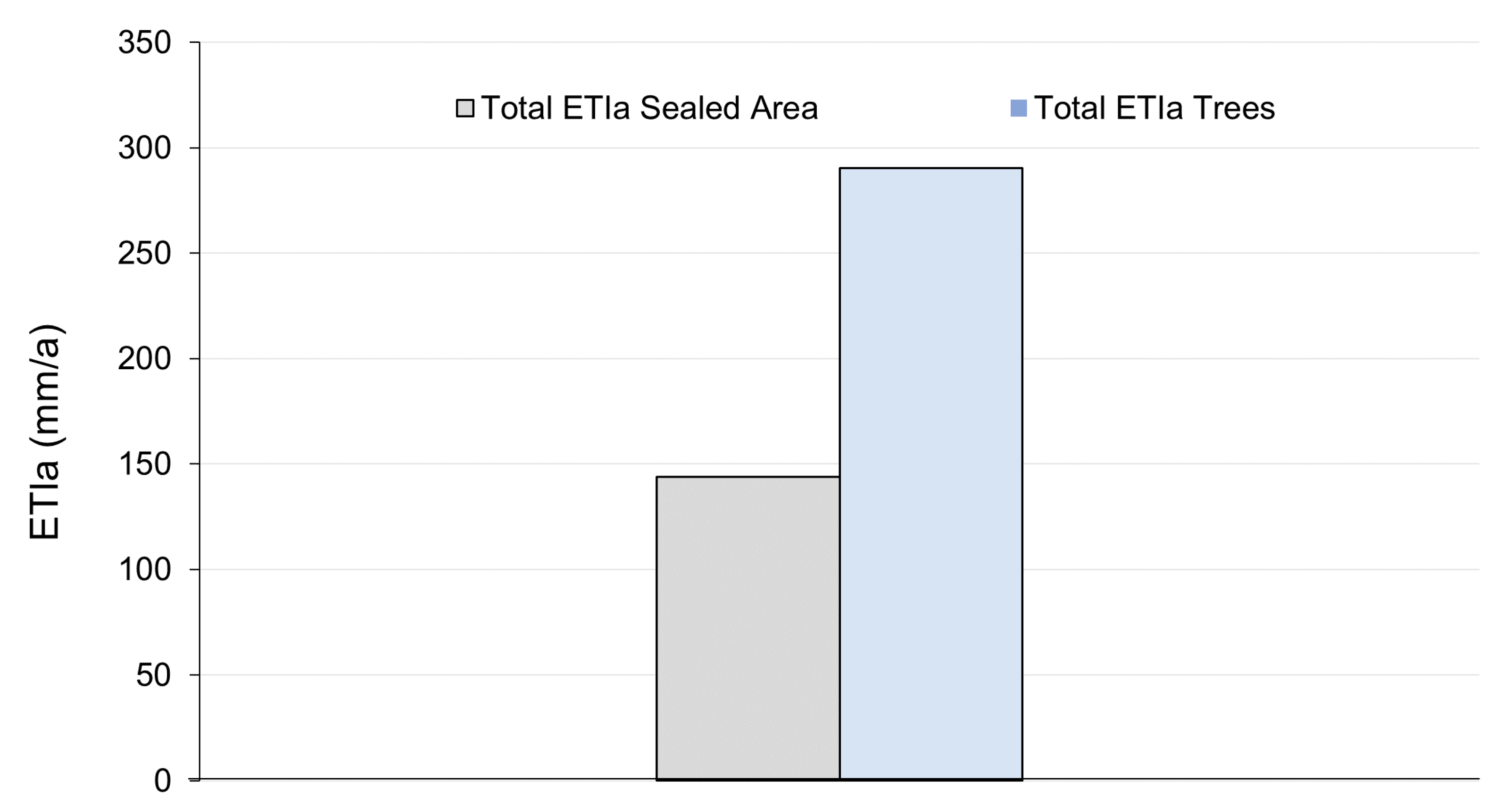
Finally, in Figure 11, an example of the long-term mean of the actual evaporation ETI_a for a street in Berlin with and without trees is presented. Actual evapotranspiration can be doubled if street trees are planted. Another important finding is that stormwater from the pavement can be reduced drastically if it is discharged and kept in the tree canopy area and not, as is usual, discharged into the street canalization. Moreover, this is a very efficient and easy applicable way to stabilize the water supply of tree, especially in dry years.

5. Conclusions

HTPFs could be a helpful tool to analyze the water supply and evapotranspiration of various street-tree situations. Both the presented concept and the equations build a good and flexible frame that is easy to program using a spreadsheet tool or an R script. Then, predictions of the site-specific water supply situations and actual evapotranspiration, as shown in our examples, cab be easily done. However, this tool should be tested and validated also for other cities and climate regions. Furthermore, uniform and comparable field and lysimeter studies to derive calibrated and validated values for common street trees are not yet available. This would be a worthwhile future study. Nevertheless, the HTPFs as presented here can already be taken for analyzing and optimization of actual urban site conditions.

Individual water balances for various trees show that young trees have less drought stress compared to older ones because their catchments still have enough plant available water. Catchments grow with the tree age and can participate from runoff of surrounding areas. Consequently, streets without trees have less evapotranspiration and more runoff. Thus, simply by planting trees with a deep rooting system and permeable seam materials beneath the catchment lead to an improved urban climate and stormwater reduction. For this goal we need innovative design concepts of street pavements and tree pits.

References

- Gaffin, S.R.; Rosenzweig, C.; Kong, A.Y.Y. Adapting to climate change through urban green infrastructure. Nature Clim. Chang. 2012, 2, 704. [Google Scholar] [CrossRef]
- Solomon, S.; Qin, D.; Manning, M.; Chen, Z.; Marquis, M.; Averyt, K.; Miller, H. IPCC fourth assessment report (AR4). Clim. Change 2007, 374. [Google Scholar]
- Allen, M.; Babiker, M.; Chen, Y.; de Coninck, H.; Connors, S.; van Diemen, R.; Ferrat, M. Summary for policymakers. In Global Warming of 1.5 C: An IPCC Special Report on the Impacts of Global Warming of 1.5 C Above Pre-Industrial Levels and Related Global Greenhouse Gas Emissions Pathways, in the Context of Strengthening the Global Response to the Threat of Climate Change; World Meteorological Organization: Geneva, Switzerland, 2018. [Google Scholar]
- Southworth, M. Designing the walkable city. J. Urban Plan. Dev. 2005, 131, 246–257. [Google Scholar] [CrossRef]
- Livesley, S.J.; McPherson, G.M.; Calfapietra, C. The urban forest and ecosystem services: Impacts on urban water, heat, and pollution cycles at the tree, street, and city scale. J. Environ. Qual. 2016, 45, 119–124. [Google Scholar] [CrossRef] [PubMed]
- Nowak, D.J.; Randler, P.B.; Greenfield, E.J.; Comas, S.J.; Carr, M.A.; Alig, R.J. Sustaining America’s urban trees and forests: A Forests on the Edge report. Gen. Tech. Rep. 2010. [Google Scholar] [CrossRef] [Green Version]
- Heisler, G.M. Effects of individual trees on the solar-radiation climate of small buildings. Urban Ecol. 1986, 9, 337–359. [Google Scholar] [CrossRef] [Green Version]
- Zhang, B.; Gao, J.X.; Yang, Y. The cooling effect of urban green spaces as a contribution to energy-saving and emission-reduction: A case study in Beijing, China. Build. Environ. 2014, 76, 37–43. [Google Scholar] [CrossRef]
- Tan, Z.; Lau, K.K.L.; Ng, E. Urban tree design approaches for mitigating daytime urban heat island effects in a high-density urban environment. Energy Build. 2016, 114, 265–274. [Google Scholar] [CrossRef]
- Shackleton, C. Do indigenous street trees promote more biodiversity than alien ones? Evidence using mistletoes and birds in South Africa. Forests 2016, 7, 134. [Google Scholar] [CrossRef] [Green Version]
- Wood, E.M.; Esaian, S. The importance of street trees to urban avifauna. Ecol. Appl. 2020, 30, e02149. [Google Scholar] [CrossRef]
- Xiao, Q.; McPherson, E.G.; Ustin, S.L.; Grismer, M.E.; Simpson, J.R. Winter rainfall interception by two mature open-grown trees in Davis, California. Hydrol. Process. 2000, 14, 763–784. [Google Scholar] [CrossRef]
- Tallis, M.; Taylor, G.; Sinnett, D.; Freer-Smith, P. Estimating the removal of atmospheric particulate pollution by the urban tree canopy of London, under current and future environments. Landsc. Urban Plan. 2011, 103, 129–138. [Google Scholar] [CrossRef]
- Berland, A.; Shiflett, S.A.; Shuster, W.D.; Garmestani, A.S.; Goddard, H.C.; Herrmann, D.L.; Hopton, M.E. The role of trees in urban stormwater management. Landsc. Urban Plan. 2017, 162, 167–177. [Google Scholar] [CrossRef] [PubMed] [Green Version]
- Lee, H.; Mayer, H.; Chen, L. Contribution of trees and grasslands to the mitigation of human heat stress in a residential district of Freiburg, Southwest Germany. Landsc. Urban Plan. 2016, 148, 37–50. [Google Scholar] [CrossRef]
- Rahman, M.A.; Armson, D.; Ennos, A.R. A comparison of the growth and cooling effectiveness of five commonly planted urban tree species. Urban Ecosyst. 2015, 18, 371–389. [Google Scholar] [CrossRef]
- Nowak, D.J.; Kuroda, M.; Crane, D.E. Tree mortality rates and tree population projections in Baltimore, Maryland, USA. Urban For. Urban Green. 2004, 2, 139–147. [Google Scholar] [CrossRef] [Green Version]
- Hanel, M.; Rakovec, O.; Markonis, Y.; Máca, P.; Samaniego, L.; Kyselý, J.; Kumar, R. Revisiting the recent European droughts from a long-term perspective. Sci. Rep. 2018, 8, 9499. [Google Scholar] [CrossRef]
- Von Berlin, A. Drucksache 18 /21 605. Schriftliche Anfrage des Abgeordneten Daniel Buchholz vom 14. November 2019 (Eingang beim Abgeordnetenhaus am 14 November 2019) zum Thema: Berliner Stadtbäume: Droht nach zwei Hitzesommern ein Kahlschlag? Senatsverwaltung von Berlin: Berlin, Germany, 2019. (In German) [Google Scholar]
- Von Berlin, A. Drucksache 18 /21 585. 2019. Schriftliche Anfrage des Abgeordneten Georg P. Kössler (GRÜNE) vom 12. November 2019 (Eingang beim Abgeordnetenhaus am 14. November 2019) zum Thema: Baumbewässerung in Berlin; Senatsverwaltung von Berlin: Berlin, Germany, 2019. (In German) [Google Scholar]
- Department of International Economic, United Nations; Department for Economic, United Nations. Social Information, & Policy Analysis. In World Population Prospects; Department of International, Economic and Social Affairs: New York, NY, USA, 1985. [Google Scholar]
- Wessolek, G.; Duijnisveld, W.H.M.; Trinks, S. Hydro-Pedo-Transfer-Functions (HPTFs) for predicting annual percolation rate on a regional scale. J. Hydrol. 2008, 356, 17–27. [Google Scholar] [CrossRef]
- Rijtema, P.E. On the relation between transpiration, soil physical properties and crop production as a base for water supply plans. Tech. Bull. Inst. Land Water Manag. Res. 1968, 58, 29–35. [Google Scholar]
- Plagge, R. Bestimmung der Ungesättigten Hydraulischen Leitfähigkeit im Boden. Ph.D. Thesis, Technische Universität Berlin, Berlin, Germany, 1991. [Google Scholar]
- Allen, R.G.; Smith, M.; Perrier, A.; Pereira, L.S. An update for the definition of reference evapotranspiration. ICID Bull. 1994, 43, 1–34. [Google Scholar]
- Federal Ministry for the Environment, Nature Conservation and Nuclear Safety. Hydrological Atlas of Germany. 2003. Available online: http://www.hydrology.uni-freiburg.de/forsch/had/had_home.htm (accessed on 22 April 2021).
- Schmidt-Walter, P.; Ahrends, B.; Mette, T.; Puhlmann, H.; Meesenburg, H. NFIWADS: The water budget, soil moisture, and drought stress indicator database for the German National Forest Inventory (NFI). Ann. For. Sci. 2019, 76, 39. [Google Scholar] [CrossRef] [Green Version]
- Duthweiler, S.; Pauleit, S.; Rötzer, T.; Moser, A.; Rahman, M.; Stratopoulos, L.; Zölch, T. Untersuchungen zur Trockenheitsverträglichkeit von Stadtbäumen. In Jahrbuch der Baumpflege; Haymarket Media GmbH: Braunschweig, Germany, 2017; pp. 137–154. ISBN 978-3-87815-253-8. (In German) [Google Scholar]
- Gillner, S.; Vogt, J.; Tharang, A.; Dettmann, S.; Roloff, A. Role of street trees in mitigating effects of heat and drought at highly sealed urban sites. Landsc. Urban Plan. 2015, 143, 33–42. [Google Scholar] [CrossRef]
- Roloff, A. Stadt- und Straßenbäume der Zukunft—Welche Arten sind geeignet? Forstwiss Beiträge Tharandt 2013, 14, 173–187. (In German) [Google Scholar]
- Renger, M.; Strebel, O. Transport von Wasser und Nährstoffen an die Pflanzenwurzel als Funktion der Tiefe und der Zeit. Mitt. Dtsch. Bodenkundl. Ges. 1982, 23, 77–88. (In German) [Google Scholar]
- Wessolek, G. Bodenwasserhaushalt. In Hydrologie; Fohrer, N., Bormann, H., Miegel, K., Casper, M., Eds.; Haupt Verlag: Stuttgart, Germany, 2016; Volume 4513, pp. 69–90. ISBN 978-3-8252-4513-9. (In German) [Google Scholar]
- ATV-DVWK. Ermittlung der Verdunstung von Land- und Wasserflächen. In Merkblätter zur Wasserwirtschaft; Deutscher Verband für Wasserwirtschaft und Kulturbau e.V.: Bonn, Germany, 1996; Volume 238, 135p, ISBN 3-89554-034-X-Heft238/1996. (In German) [Google Scholar]
- Senatsverwaltung für Stadtentwicklung und Wohnen. Umweltatlas Berlin. Available online: https://fbinter.stadt-berlin.de/fb/index.jsp?loginkey=zoomStart&mapId=k_wfs_baumbestand@senstadt (accessed on 4 March 2021).
- Gong, F.Y.; Zeng, Z.C.; Zhang, F.; Li, X.; Ng, E.; Norford, L.K. Mapping sky, tree, and building view factors of street canyons in a high-density urban environment. Build. Environ. 2018, 134, 155–167. [Google Scholar] [CrossRef]
- Koelbing, M.; Schuetz, T.; Weiler, M. Downscaling potential evapotranspiration to the urban canyon. Hydrol. Earth Syst. Sci. Discuss. 2021. [Google Scholar] [CrossRef]
- Costello, L.R.; Matheny, N.P.; Clark, J.R. WUCOLS III: A Guide to Estimating Irrigation Waterneeds of Landscape Plantings in California: The Landscapecoefficient Method. San Mateo and San Francisco Counties: University of California Cooperative Extension, California Department of Water Resources. 2000. Available online: https://sanmarprop.com/assets/pdf/wucols00.pdf (accessed on 22 April 2021).
- Coutts, A.M.; White, E.C.; Tapper, N.J.; Beringer, J.; Livesley, S.J. Temperature and human thermal comfort effects of street trees across three contrasting street canyon environments. Theor. Appl. Climatol. 2016, 124, 55–68. [Google Scholar] [CrossRef]
- Watson, I.D.; Johnson, G.T. Graphical estimation of sky view-factors in urban environments. J. Climatol. 1987, 7, 193–197. [Google Scholar] [CrossRef]
- Bohne, K. Monitoring zum Wasserhaushalt einer auf litoralem Versumpfungsmoor gewachsenen Regenmoorkalotte. In Aspekte der Geoökologie; Stüdemann, O., Ed.; Weißensee-Verlag: Berlin, Germany, 2008; pp. S313–S336. ISBN 978-3-89998-127-8. (In German) [Google Scholar]
- Schwärzel, K.; Bohl, H.P. An easily installable groundwater lysimeter to determine water balance components and hydraulic properties of peat soils. Hydrol. Earth Syst. Sci. 2003, 7, 23–32. [Google Scholar] [CrossRef]
- QGIS.org. QGIS Geographic Information System. 2021. QGIS Association. Available online: http://www.qgis.org (accessed on 22 January 2021).
- Lindberg, F.; Grimmond, C.S.B.; Gabey, A.; Huang, B.; Kent, C.W.; Sun, T.; Zhang, Z. Urban Multi-scale Environmental Predictor (UMEP): An integrated tool for city-based climate services. Environ. Model. Softw. 2018, 99, 70–87. [Google Scholar] [CrossRef]
- Matzarakis, A.; Rutz, F.; Mayer, H. Modelling Radiation fluxes in simple and complex environments—Basics of the RayMan model. Int. J. Biometeorol. 2010, 54, 131–139. [Google Scholar] [CrossRef] [PubMed] [Green Version]
- Wessolek, G. Empfindlichkeitsanalyse eines Bodenwasser-Simulationsmodells. Mitt. Deutsch. Bodenkundl. Ges. 1983, 38, 165–171. (In German) [Google Scholar]
- Renger, M.; Bohne, K.; Facklam, M.; Harrach, T.; Riek, W.; Schäfer, W.; Wessolek, G.; Zacharias, S. Bodenphysikalische Kennwerte und Berechnungsverfahren für die Praxis. In Bodenökologie und Bodengenese; Techn. Universität: Berlin, Germany, 2009; 80p, Available online: https://www.researchgate.net/publication/294427537_Bodenphysikalische_Kennwerte_und_Berechnungsverfahren_fur_die_Praxis/link/56c0c55c08ae2f498ef99662/download (accessed on 22 April 2021). (In German)
- Vereecken, H.; Feyen, J.; Maes, J.; Darius, P. Estimating the soil moisture retention characteristic from texture, bulk density and carbon content. Soil Sci. 1989, 148, 389–403. [Google Scholar] [CrossRef]
- Wösten, J.H.M.; Lilly, A.; Nemes, A.; Le Bas, C. Development and use of a database of hydraulic properties of European soils. Geoderma 1999, 90, 169–185. [Google Scholar] [CrossRef]
- Zacharias, S.; Wessolek, G. Excluding organic matter content from pedotransfer predictors of soil water retention. Soil Sci. Soc. Am. J. 2007, 71, 43–50. [Google Scholar] [CrossRef]
- Breuste, J.; Keidel, T.; Meinel, G.; Münchow, B.; Netzband, M.; Schramm, M. On analyzing and predicting surface sealing. In UFZ-Leipzig Report of Ecological Studies; UFZ-Leipzig: Leipzig, Germany, 1996; Volume 7, 230p, ISSN 0948-9452. (In German) [Google Scholar]
- Boden, A.G. Ad-hoc-Arbeitsgruppe Boden der Geologischen Landesämter und der Bundesanstalt für Geowissenschaften und Rohstoffe der Bundesrepublik Deutschland. Aufl. Nachdr. 2005, 4, 392. (In German) [Google Scholar]
- Flöter, O. Wasserhaushalt Gepflasterter Strassen und Gehwege. Lysimeterversuche an Drei Aufbauten unter Praxisnahen Bedingungen unter Hamburger Klima. Ph.D. Thesis, Universität Hamburg, Hamburg, Germany, 2006. (In German). [Google Scholar]
- Wessolek, G.; Facklam, M. Standorteigenschaften und Wasserhaushalt von versiegelten Flächen. J. Plant. Nutr. Soil Sci. 1997, 160, 41–46. [Google Scholar] [CrossRef]
- Nehls, T.; Jozefaciuk, G.; Sokolowska, Z.; Hajnos, M.; Wessolek, G. Pore-system characteristics of pavement seam materials of urban sites. J. Plant Nutri. Soil Sci. 2006, 169, 16–24. [Google Scholar] [CrossRef] [Green Version]
- Gillner, S. Stadtbäume im Klimawandel-Dendrochronologische und Physiologische Untersuchungen zur Identifikation der Trockenstressempfindlichkeit Häufig Verwendeter Stadtbaumarten in Dresden. Ph.D. Thesis, Technische Universität Dresden, Dresden, Germany, 2012. (In German). [Google Scholar]
- De Jaegere, T.; Hein, S.; Claessens, H. A review of the characteristics of small-leaved lime (Tilia cordata Mill.) and their implications for silviculture in a changing climate. Forests 2016, 7, 56. [Google Scholar] [CrossRef] [Green Version]
- Rahman, M.A.; Moser, A.; Anderson, M.; Zhang, C.; Rötzer, T.; Pauleit, S. Comparing the infiltration potentials of soils beneath the canopies of two contrasting urban tree species. Urban For. Urban Green. 2019, 38, 22–32. [Google Scholar] [CrossRef]
- Granier, A. Evaluation of transpiration in a Douglas-fir stand by means of sap flow measurements. Tree Physiol. 1987, 3, 309–320. [Google Scholar] [CrossRef] [PubMed]
- DWD Climate-Data-Center. Historical Hourly Station Observations of 2m Air Temperature and Humidity for Germany, version 006; DWD Climate Data Center: Offenbach am Main, Germany, 2018. [Google Scholar]
- SenStadtWohn—Senatsverwaltung für Stadtentwicklung und Wohnen Berlin. Umweltatlas Berlin. Ausgabe. 2020. Available online: https://www.stadtentwicklung.berlin.de/umwelt/umweltatlas/ (accessed on 1 February 2021).
- Steppe, K.; De Pauw, D.J.W.; Doody, T.M.; Teskey, R.O. A comparison of sap flux density using thermal dissipation, heat pulse velocity and heat field deformation methods. Agric. For. Meteorol. 2010, 150, 1046–1056. [Google Scholar] [CrossRef]
- Fuchs, S.; Leuschner, C.; Link, R.; Coners, H.; Schuldt, B. Calibration and comparison of thermal dissipation, heat ratio and heat field deformation sapflow probes for diffuse-porous trees. Agric. For. Meteorol. 2017, 244–245, 151–161. [Google Scholar] [CrossRef]
Figure 1.
Examples of urban street-tree catchments, as found in Mexico City, Paris, NYC, Sydney, and Berlin.
Figure 2.
Principal HTPF concept: ETIa/ET0 (-) is the ratio of actual and potential evapotranspiration as a function of the total water supply (Sw). While Function 1 is to be used for sites with water limitation, Function 2 is suitable for sites without any water limitation. The threshold of an unlimited water supply for trees in the eastern part of Germany is about 800 mm. The three lines (I, II, and III) of both functions indicate various levels of ET0.
Figure 3.
HPTF validation by comparisons of the gauge-measured values with the predicted percolation rate + runoff, taken in 106 catchments areas in Germany [22].
Figure 4.
Scheme for characterizing the site conditions of a street tree.
Figure 5.
Potential daily capillary rises rates (Qpot) in mm/d as a function of the distance between the groundwater table and effective root zone for different soil textures according to the German Soil Classification System [51].
Figure 6.
Grass reference evapotranspiration of the summer half years (Eo,s) related to values of the entire year (ET0).
Figure 7.
Scheme for surface runoff (Ro), which either can be a loss or a gain for the tree pit.
Figure 8.
Three Linden trees (Tilia cordata) used for sap-flow measurements. Left: Young (in 2017) planted tree growing in a steel lysimeter in the center of an experimental station of the UBA in Berlin-Marienfelde. Middle: 30–40-year-old tree growing in a park-like situation not far away. Right: 35-year-old street tree that was used in 2017 for the sap-flow measurements by Rahman et al. [57].
Figure 9.
Mean water supply, Sw (mm) per m2 catchment area of 20 trees at Kufsteiner Straße in Berlin, mapped by using the parameters listed in Table 2. The black line indicates the average Sw of all catchments. In red color: additional runoff to the tree pit increases the Sw.
Figure 10.
Long-term mean actual evapotranspiration, ETIa (mm/a) per m2 catchment of the street trees at the Kufsteiner Straße, Berlin, Germany.
Figure 11.
Mean actual evapotranspiration ETIa (mm/a) for a street without (left) and with street trees (right) in Berlin.