Climate Associations with Headwater Streamflow in Managed Forests over 16 Years and Projections of Future Dry Headwater Stream Channels

1
Pacific Northwest Research Station, US Forest Service, 3200 SW Jefferson Way, Corvallis, OR 97331, USA
2
Department of Forest and Natural Resources Management, SUNY College of Environmental Science and Forestry, Syracuse, NY 13210, USA
*
Author to whom correspondence should be addressed.
†
These authors contributed equally to this work.
Forests 2019, 10(11), 968; https://doi.org/10.3390/f10110968
Submission received: 29 September 2019
/
Revised: 27 October 2019
/
Accepted: 30 October 2019
/
Published: 2 November 2019
(This article belongs to the Special Issue Managing Forests and Water for People under a Changing Environment)
Abstract
:Integrating climate-smart principles into riparian and upland forest management can facilitate effective and efficient land use and conservation planning. Emerging values of forested headwater streams can help forge these links, yet climate effects on headwaters are little studied. We assessed associations of headwater discontinuous streams with climate metrics, watershed size, and forest-harvest treatments. We hypothesized that summer streamflow would decrease in warm, dry years, with possible harvest interactions. We field-collected streamflow patterns from 65 discontinuous stream reaches at 13 managed forest sites in Western Oregon, USA over a 16-year period. We analyzed spatial and temporal variability in field-collected stream habitat metrics using non-metric multidimensional scaling ordination. Relationships between streamflow, climate metrics, basin size, and harvest treatments were analyzed with simple linear models and mixed models with repeated measures. Using past effects of climate variation on streamflow, we projected effects to 2085 under three future scenarios, then quantified implications on headwater networks for a case-study landscape. Ordination identified the percent dry length of stream reaches as a top predictor of spatial and temporal variation in discontinuous stream-habitat types. In our final multivariate model, the percent dry length was associated with heat: moisture index, mean minimum summer temperature, and basin area. Across future climate scenarios in years 2055–2085, a 4.5%–11.5% loss in headwater surface streamflow was projected; this resulted in 597–2058 km of additional dry channel lengths of headwater streams in our case study area, the range of the endemic headwater-associated Cascade torrent salamander (Rhyacotriton cascadae Good and Wake) in the Oregon Cascade Range, a species proposed for listing under the US Threatened and Endangered Act. Implications of our study for proactive climate-smart forest-management designs in headwaters include restoration to retain surface flows and managing over-ridge wildlife dispersal habitat from areas with perennial surface water flow, as stream reaches with discontinuous streamflow were projected to have reduced flows in the future with climate change projections.
1. Introduction
Land managers addressing forest ecosystem sustainability face complex challenges of integrating societal and ecological objectives for myriad natural resources that are prioritized as ecosystem services, inclusive of wood, water, species, and cultural factors [1,2,3]. Historically, disturbances managed relative to forest ecosystems have been related primarily to resource extraction approaches that retain designated priorities such as ecological structures, processes or functions (e.g., Pacific Northwest moist coniferous forests [4]). Contemporary forest landscape planners are managing these factors in addition to considering documented effects of climate variability and projections of climate change on forest resources and ecosystems for the development of climate-smart forest-management designs [5]. Although new information is now accumulating regarding how spatio-temporal variability in climate metrics intersect with various individual forest ecosystem services [6], integration of studies across forest taxonomic and ecosystem boundaries is needed to address combined management and ecological efficiencies. In particular, integration of forest ecosystem-management approaches for both aquatic- and upland terrestrial systems relative to the known effects of climate variability and potential futures of climate change is of paramount importance.
A division between aquatic- and upland-management planning in forests has been evident, as natural resource specialists have addressed their areas of expertise separately (e.g., fish biology and aquatic ecology, wildlife biology, forest-stand management), before assembling their individual pieces into a larger project or landscape plan. This approach can be seen in the development of best management practices (BMPs) in the United States that have targeted different legal requirements for each category of resource, such as streamside buffer zones to address water-quality standards (e.g., the US Clean Water Act), habitat set-asides for sensitive-species protections (e.g., the US Endangered Species Act), and multi-resource environmental assessments conducted to support forestry practices (e.g., the US National Forest Management Act). However, adaptive management of these processes to better integrate the separate pieces as well as incorporating new knowledge as it becomes available is an essential piece of forest-landscape management. For example, the recent update to the US Forest Service’s Planning Rule [7] includes new language about management of broader ecosystem services as well as addressing integration of forest landscape issues such as habitat connectivity, watershed protection, wildlife conservation, and resilience to climate change.
Furthermore, renewed recognition that both aquatic-riparian areas and uplands in forests are heterogeneous systems over space and time has emerged from US Pacific Northwest forest syntheses [8,9,10], adding complexity to broader forest landscape sustainability goals, integration across ecosystems therein, and management of climate-smart forests [5,6]. Spatiotemporal complexity can be generated by gradients in conditions (e.g., with geographic, geologic and hydrologic conditions, also with latitude, distance from coastal mesic influence, rain-shadows) as well as repeated pulse disturbances, some of which have their roots in extreme climate events (e.g., wind-throw, ice damage, drought, flood) and can be aggravated by human activities (e.g., fire and past fire suppression; past timber-harvest practices including tree cutting and road and culvert construction affecting erosion and debris-flow events). Dynamic forested ecosystems are especially evident from our increasing knowledge of unique species and species-assemblages that result from disturbances, species interactions, and species’ life-history variation including dispersal limitations. In the US Pacific Northwest, this is exemplified by the number of rare or little known late-successional forest species that are afforded site-specific protection under the Northwest Forest Plan survey-and-manage provision [11,12,13].
Forested headwaters have been proposed as ideal places for the intersection of aquatic-riparian and upslope management for ecological sustainability ideals such as biodiversity management, and can also be useful to address dynamic forest ecosystems under climate change [14,15,16]. In forests of montane landscapes, topographic relief is responsible for numerous headwater streams extending toward ridgelines throughout watersheds, with the spatial extent of headwater streams encompassing 50–80% of forested watersheds [17,18,19,20]. This affects the riparian-upland forest areas designated to buffer stream values, such as stream-buffer provisions extending to ~70- to 140-m away from streams on federal lands managed under the United States’ federal Northwest Forest Plan [21], resulting in an increased focus on the ecological values of headwaters and a need to better understand management practices for sustainability of natural resources for ecosystem integrity and commodity production. Headwater values include distinct floral and faunal composition or structure [22,23,24,25,26,27,28,29,30,31] and headwater connectivity to downstream aquatic-riparian networks for the delivery of down wood [32,33,34] and sediment [34,35,36,37] for habitat structure, contributions of cool water for cold-adapted northwest fauna such as economically-important salmonid fishes [19,38,39], and prey for downstream fish communities [40]. Headwaters offer upland connectivity opportunities as well, as they often are the closest areas to ridgelines, and over-ridge habitat connectivity to adjacent watersheds [15,16]. For the conservation principle of redundancy of protections, an especially important tenet when systems are dynamic in nature, the multitude of headwaters provide an opportunity for managing redundant headwater stream reaches—for persistence of their associated in situ populations per reach or reach-network, as well as for dispersal habitat connections over ridgelines or downstream. For aquatic-riparian dependent species as well as terrestrial species, dispersal routes along riparian corridors can funnel individuals into narrowing headwaters before a relatively short over-ridge distance can be traversed to a novel watershed; for example, aquatic and terrestrial amphibians may move along headwater riparian areas, disperse over forested ridges, and retain gene flow among populations in adjacent watersheds [16,41,42].
In the Pacific Northwest, in particular, assessments of climate variability and projections of climate change in forested headwaters are important owing to the dominance of these drainages in the landscape, and their importance to multiple downstream and upland ecosystem services—yet we are just beginning to understand climate influences on forested headwater streams. Stream-temperature and streamflow changes are attributes often considered in watershed studies of climate change, as these factors affect stream ecological conditions and functions, especially species habitat suitability via myriad ecophysiological constraints [38,39,43]. In the Northwestern US more generally, at larger scales (i.e., larger landscapes and watersheds), climate projections include warmer temperatures [44,45,46,47] and altered precipitation patterns such as reduced snowpack—especially at low-to-mid elevations [48,49], which have many headwater basins in the region. These changes may affect streamflow, in particular, which is also driven by landscape-scale drainage efficiency in converting precipitation to discharge [50,51,52]. A sensitivity map for summer streamflow across Oregon and Washington, USA showed variable patterns with geographic conditions, including areas in the Cascade Range being particularly vulnerable to low summer streamflows owing to volcanic geology with deep groundwater systems [52]. Runoff- and groundwater-dominated watersheds contrast, with groundwater-dominated streams being especially sensitive to changes in snowmelt amount and timing [53]. Less focus on understanding variation in headwater streamflow patterns has occurred, as so far the focus has been on examining watersheds at larger scales, with field streamflow measurements more often assessed at downstream tributary junctions. Discontinuous streamflows in headwater stream reaches can translate to logistical challenges for stream gaging methods that are often used for surface-flow pattern assessment.
Interactions of local geographic conditions with forest-vegetation and stream size are also important considerations for streamflow dynamics. Upland forest management can affect streamflows: generally, timber harvest is thought to decrease evapotranspiration, increasing soil moisture storage, runoff, and streamflows, with patterns following intensity of disturbance and catchment area effects [54,55,56,57,58,59,60]. Yet patterns and processes may vary with site conditions (e.g., climate, soils, topography, vegetation type, harvest type, time since harvest, season [54,59,61], and general forest ecosystem type: (1) in mesic systems, increased streamflow may result from reduced canopy interception of precipitation and evapotranspiration, leading to more water draining towards stream channels, especially in wet seasons; (2) in arid systems, there may be less change in flow in all but the wettest systems owing to different processes of rainfall interception, soil saturation, and vaporization; and (3) in subalpine systems with arid summers, there may be little response in summer but increased flows during snowmelt [62]. Relative to streams in small watersheds in the Pacific Northwest moist coniferous zone, a pattern of increased streamflow following harvest has been supported [61,63,64]. For example, in one study [63], previously intermittent streams became perennial, and summer streamflow enhancement was attributed to increased zones of deep perennial saturation. Conversely, another study reported lower streamflow in small streams in 34- to 43-year-old plantations, compared to older forests (150–500 years old) [65], suggesting an uncertain amount of variation may be occurring at local scales and perhaps with past site histories. At this time we have limited knowledge regarding the comparative magnitudes of timber-harvest and climate-variation effects on streamflows, or their interactions. However, a study of streamflows in Arizona, USA forests reported forest changes were associated with streamflow variation to an extent similar to that of climate variability [66].
Understanding how climate variation and forest management interact with streamflow patterns in basins of different sizes and geographic contexts, and consequent effects on other stream resources such as biota, involves a complex web of interactions that is gaining research and management attention. With increasing risks to natural resources from joint disturbances including forest-management practices and climate change projections, studies of the dynamic contexts and consequences of multiple-threat interactions are becoming more important [67]. Aquatic-dependent biota, in particular, are fast-declining and have been considered a ‘weak link’ in forest ecosystem integrity [8]; they deserve heightened attention for the interactive threats of habitat loss from anthropogenic disturbance and climate change projections, two of their most important risk factors today. Forested headwater streams and their associated riparian areas provide important reproductive, foraging, and dispersal habitat for unique assemblages of forest-dependent species, especially endemic amphibian species in Pacific Northwest moist coniferous forests [25,68]. Previous studies have shown that the composition of aquatic and riparian animal communities in northwest forests is associated with habitat characteristics of headwater reaches, with unique assemblages associated with both perennial-continuous and intermittent-discontinuous portions of headwater stream networks, e.g., Western Oregon: [24,25,68,69]. However, relationships between headwater streamflows, climate, forest management, and geographic contexts is not well examined by empirical studies.
To advance our understanding of the joint effects of climate and forest management on stream surface flows in small headwater basins, we conducted a retrospective study with summer low-flow data over 16 years, field-collected from headwater streams with discontinuous water flow in forest stands subjected to an experimental harvest regime in Western Oregon, USA. We hypothesized that summer dry-season headwater surface-flow stream lengths would be reduced in past years with reduced precipitation and warmer temperatures. But we also predicted that there could be a signature of the upland forest-harvest regime on summer headwater streamflows, with potentially increased flows in headwater streams having the narrowest streamside riparian buffers (three buffer widths assessed, and unharvested reference streams) in areas with upland thinning and hence relatively more upland soil saturation and perennial runoff. We projected that interactions of buffers and climate might occur, but did not predict an outcome because we had little a priori basis for understanding relative magnitudes of these dual effects for headwater stream drainages in our study area. We also considered headwater basin area per stream reach as a geographic variable affecting streamflow, with larger basins likely collecting more precipitation and having more discharge and surface streamflows. We then used our empirical findings from field-collected surface streamflow patterns collected over this 16-year time interval, along with annual climate variability, to parameterize models of landscape-scale climate change to project effects into the future. Future climate projections for a case-study forested landscape area were then computed to assess potential cumulative effects of changes to headwater surface streamflow patterns, especially relevant to aquatic-dependent forest species with headwater associations. We used the range of the Cascade torrent salamanders (Rhyacotriton cascadae Good and Wake), a headwater-associated species found in discontinuous streams in the Cascade Range that is proposed for listing under the USA Endangered Species Act, to exemplify the potential consequences of headwater surface streamflow changes. We used this salamander to represent the larger assemblage of biota in the uppermost headwater habitats of these stream systems in young forests at low to mid-elevations. For example, faunal assemblages at headwater streams at our study sites also have been previously described as unique due to increased density and biomass of Diptera (flies) [24].
2. Methods
2.1. Study Area
This project is part of the larger Density Management and Riparian Buffer Study examining the effects of variable thinning intensities and riparian buffer widths on aquatic and riparian vertebrates and their habitats in headwater streams in Western Oregon [68,70]. The 13 sites studied here were distributed on forestlands managed by the United States Department of the Interior Bureau of Land Management (BLM) and Department of Agriculture Forest Service along the Coast and Cascade Ranges in Western Oregon (Figure 1). Sites were located in the western hemlock vegetation zone, characterized by mild, wet winters and warm, dry summers [71]. Forests were dominated by Douglas-fir (Pseudotsuga menziesii (Mirbel) Franco), western hemlock (Tsuga heterophylla (Raf.) Sarg.); co-dominant species at three Cascade Range study sites, and contained varying abundances of hardwood species such as big-leaf maple (Acer macrophyllum Pursh), red alder (Alnus rubra Bong.), and golden chinquapin (Chrysolepis chrysophylla (Douglas ex Hook.) Hjelmqvist). Site selection was nonrandom, but was intended to represent young-managed stands on different BLM and Forest Service management units, and were stands with homogenous vegetation conditions and specified stand ages. All sites were naturally regenerated to ~430–890 trees per hectare (tph) after primary late-successional and old-growth (LSOG) stands were clearcut 30–80 years prior to the initiation of our Study, without stream buffers during that initial harvest. At the onset of our study, 10 sites were 30–50 years old, three sites were 70–80 years old (additional site information: [68,70]). Two sites with forest-stand ages 70–80 years were previously thinned to 250 tph when they were at secondary forest-stand ages of 50 years (Perkins Creek, North Ward), hence our study was the second entry for density management harvest at these two sites. At these sites, recent mean annual temperature ranges from 9 °C to 12 °C, mean annual precipitation ranged from 121.7 cm to 301.9 cm, with the growing season ranging from 271 to 326 frost-free days (Climate WNA (Western North America), 1961–1990 average, a time period framing considerable stand development at these sites) [72,73,74]. Elevation ranges from 183 m to 700 m above sea level among sites.
2.2. Experimental Design
Small stream channels consisting of narrow first- and second-order headwater streams dissected the forested uplands at each site. The experimental/observational unit examined here is the stream reach. The uppermost extent of a stream reach was most often (80% of the time) defined by the upstream end of surface streamflow in the wet spring season (~March–May), such that no surface flow was observed from that point to the ridgeline during the wettest times sampled. Less frequently (20% of the time), the uppermost study stream reach was delineated by a study site or treatment boundary. The downstream end of a study reach usually was defined by the stream extending into a different treatment, out of the study site, or by an intersection with another stream. Different geometries of stream networks and upland harvest implementation within study drainages resulted in stream-reach lengths ranging between 70 m and 687 m.
All study stream reaches had dry channel sections between upstream and downstream flowing sections. For this reason, rather than referring to our study reaches as being perennial or ephemeral, which suggests always-flowing or seasonally flowing streams, our small headwater streams were better classified by hydro-typing their surface flows as continuous or discontinuous, spatially, or seasonally [68]. Most stream reaches in our study were spatially discontinuous (i.e., spatially intermittent) [68]. In the spring wet season, they had surface flow at the upper and lower reach ends with intervening areas in the middle where the surface channel went dry. In the summer dry season, this spatial intermittency was retained, but dry channels were extended in length in the middle and top-most part of the reaches. This field observation was a particular incentive for our study to examine the potential influence of climate factors on surface flow. Perennial reaches (continuous flow) occurred in larger stream reaches downstream, but we rarely saw streams we would call ephemeral or seasonal, being continuous in the wet season and then going completely dry or subsurface along their upmost reach extent during summer dry seasons. Hence, we only analyzed spatially intermittent channels in this study, resulting in a total of 65 headwater reaches being sampled at the 13 study sites and included in our analyses (Table 1). It is possible that discontinuous streams are typical of our montane landscapes if multiple springs intersect the ground surface, or if the stream has become disconnected due to prior side-slope erosion causing the stream channels to have been infilled. These may not be mutually exclusive, however. We saw apparent multiple sequential headwalls occurring in some of our 65 reaches, between which intervening sections of our stream reaches went dry or subsurface, which may have occurred from erosion from previous disturbances, natural, or anthropogenic. All sites had been previously clearcut without stream buffers, and it is likely that timber yarding up or across streams disrupted substrates. Other analyses reported from our data have included perennial (continuously flowing) stream reaches and reaches that were always dry [68]; various past studies have analyzed different subsets of reaches, sites, and years [69,75,76].
Our experiment was a before-after-control-impact design at each of the 13 sites with upland forest density-management timber harvest and alternative stream-buffer treatments (Table 1). All treatment stream reaches were within a heterogeneous thinned matrix, except 18 of 65 reaches were within upland forest units that were unthinned during our study (i.e., controls). All of the remaining 47 reaches went through one (21 reaches) or two (26 reaches) sequential thinning entries as part of our study. Post-treatment year 11 to 14 (Table 1, right-most column) typically corresponded to time intervals after the second thinning. We acknowledge that nuanced effects of different upslope thinning densities in the heterogeneous upland forest matrix among sites are obscured in our analyses, but we felt there could be sufficient power to focus on the potential effects of climate metrics, riparian buffer width, and drainage area to understand streamflow variation within a forest-thinning neighborhood as described below.
Briefly, during the first thinning at 11 sites, upland density management treatments reduced overstory tree density from 430–890 tph to 100–300 tph; there were 25 reaches within an upland thinned matrix of 200 tph, 13 reaches in a 300 tpa unit, and four reaches in a unit with variable density thinning, 100–300 tph. At seven sites in the younger stand ages, 30–50 year, circular clearcut gaps and leave-tree islands (skips) of three sizes (0.1, 0.2, and 0.4 ha) were embedded in the thinned matrix. This heterogeneous pattern was designed to test methods to accelerate development of LSOG stand conditions. Three of ten sites in the younger age category (30–50 year: Cougar Creek, Grant Creek, Schooner Creek) and all three sites in the older age category (70–80 year: Callahan Creek, Perkins Creek, North Ward), were thinned without gaps and islands. At two older age class sites (Perkins Creek and North Ward) for which our experimental thinning was a second-entry harvest, our first treatment reduced overstory density from 250 tph to 100–150 tph. North Ward included an earlier once-thinned control unit in addition to a never-thinned control unit; both were unmanaged during our study and stream reaches in them were categorized as controls. A second thinning entry occurred at eight sites (upslope of 26 reaches with buffers), including Perkins Creek and all sites with the heterogeneous matrix described above. The second thinning reduced overstory density from 150–200 tph to 75 tph upslope of buffers along 20 reaches, and from 300 to 150 tph upslope of buffers along six reaches—three of these six reaches had thinned variable-width buffers during the second thinning, to 150 tph [69]. Most sites had additional thinning treatments in adjacent upland units to address upland objectives of how to accelerate LSOG [70], but were not included here due to lack of stream-buffer replication. Thinning operations generally occurred over a two-year time span during which field access was constrained. Additional harvest information is available [69,70,77].
At each site, experimental treatments of upland density management were combined with alternative riparian-buffer treatments on each side of spatially intermittent (discontinuous) streams: one site-potential tree-height buffers (~70 m; eight replicate reaches), as per the interim guidance for the federal Northwest Forest Plan in the study area for non-fishbearing intermittent streams [21]; variable-width buffers (≥15 m; 26 replicate reaches) which widened with site conditions such as steep inner gorges, side-slope seeps, and unique vegetation such as old ‘wolf’ trees retained from the initial clearcut; and streamside-retention buffers (~6 m; 13 replicates), intended to retain streamside tree roots to reduce erosion to streams and provide direct overstory shading of stream channels. Spatially intermittent stream reaches within untreated control units (18 replicates) were also sampled at sites to provide a reference for the effects of our upland thinning and riparian-buffer treatments.
Most sites were small headwater basins, and had size and stream geometry constraints for implementation of a fully randomized design of buffer treatments. We aimed for a minimum 60-m distance between the upslope edge of the buffer and the ridgeline of the basin to accommodate a thinning treatment. Some stream reaches were unable to accommodate wider buffers with thinning before the ridgeline due to their small basin size. If the wider buffer could fit, full randomization of treatments may have been compromised to allow its deployment.
2.3. Field Methods
A total of 65 stream reaches that had been identified as spatially intermittent during spring wet-season surveys were field-surveyed in the dry summer season, July–September, periodically over 16 years (1995–2011; no sampling in 2007). However, every site was not sampled each year as site harvests were implemented over a multiple-year timespan owing to coordination among different land-management districts and harvest contractors. Pre-treatment data were collected in one year at sites between 1995 and 1999, and post-treatment data were scheduled to be collected in years 1, 2, 5, and 10 years after density-management timber harvests were completed; post-treatment surveys were conducted from 1998 to 2011 (Table 1). Although we had only four post-treatment years for scheduled sampling, some post-treatment survey intervals spanned additional years due to site-access constraints such as harvest operations within sites occurring across several years. For example, if we were permitted to access a stream reach immediately after upland thinning while harvest operations continued at other site areas, our timeframe of sampling may have bridged contiguous years at a site for due diligence to census conditions in the first year post-treatment as per our design. Overall, field surveys were conducted in 362 total reach x time intervals.
Stream habitat data were collected per reach during field surveys. As field personnel walked upstream, reaches were partitioned into one of three habitat unit types by three streamflow classes: riffles were dominated by faster water currents, inclusive of steeper gradient areas that might be considered steps or cascades; pools were units with surface water having little visible stream current; dry units had no surface water flow. Small headwater streams can have heterogeneous surface flow units within a single stream length, such as a small side pool along a fast-flowing riffle; these units were characterized by the dominant type along the stream length, usually the riffle because of the higher gradients at our headwater sites. Per unit, surface dimensions (length and width) were measured in the field using a meter tape, and habitat conditions such as substrate type by particle size was visually estimated (fine substrates, <3 mm diameter (diam) particles; small gravel, 3–10 mm diam; large gravel, 11–30 mm diam; cobble, 30–100 mm diam; boulder, 101–300 mm diam; bedrock, >300 mm diam). Units were measured continuously along the entire length of the reach.
2.4. Stream Reach Characteristics
From our stream habitat data we characterized 27 stream reach and surface flow attributes per reach (Table 2), from which we could determine a dominant streamflow metric for further analyses of surface flow variation. Our calculations were conducted by major surface flow type (i.e., riffle, pool, dry,), including the percentage of units and their total lengths in each flow class and the ratio of dry length to wet length (dry: Wet). We calculated both the average attributes of all units within a reach, and the coefficient of variation (cv) per attribute (Table 2). Instream habitat conditions were somewhat comparable across reaches, as shown by smaller substrates dominating reaches (Figure 2). In addition, we used a geographic information system (ArcGis desktop 10.1/10.5.1, ESRI, Redlands, CA, USA; https://www.esri.com, accessed 11 July 2019) to calculate basin areas of each of the 65 reaches to assess patterns with streamflow in our study reaches.
2.5. Climate Metrics and Future Scenarios
Seasonal and annual climate data, and future projections (i.e., 2025, 2055, and 2085) were obtained for each site based on geographic coordinates and elevation from down-scaled spatial interpolations of monthly data, accounting for effects of local topography, rain shadows, coastal influence, and temperature inversions using Climate WNA [72,73,74]. Twenty-one climate metrics were assessed (Table 3). For each site and year, annual and seasonal observed and derived climate metrics were obtained, in addition to 30-year recent conditions (i.e., 1961–1990 averages).
Future projections were developed by atmosphere–ocean general circulation models (AOGCM) from the Fifth Assessment of the Intergovernmental Panel on Climate Change [78] including the Canadian Earth System Model (CanESM2) RCP 4.5, the Model for Interdisciplinary Research on Climate (MIROC5) RCP 8.5 and the Met Office Hadley Centre HadGEM2-ES Earth System model RCP 8.5. These scenarios cover a range of uncertainty in emissions scenarios and global climate models, though most GCMs reproduce observed (historical) patterns of climate in the Pacific Northwest reasonably well [45]. The RCP 8.5 assumes CO2 emissions with emissions increasing exponentially over time, resulting in a future climate that is hot and dry. Relative to RCP 8.5, the RCP 4.5 assumes increases in CO2 emissions peak around 2040 and decrease thereafter.
2.6. Statistical Analysis
To examine the main dimensions of variation in surface streamflow, we used non-metric multidimensional scaling (NMS) ordinations of reaches, measured repeatedly over time, described by the 27 stream characteristics calculated (Table 2). NMS iteratively finds the best solution, or axes of variation, that capture patterns in the dissimilarity matrix (i.e., Sørensen measure of dissimilarity) [79]. Using rank distances, NMS is robust to non-linearities among variables and exhibits superior performance across a range of data structures as compared to other ordination techniques [80]. We first assessed dimensionality using the quick and dirty autopilot mode in PC ORD [81]. Then we ran the ordination starting from a random configuration specifying the suggested number of dimensions (k = 3), 50 runs with real data, 50 iterations to evaluate stability, initial step length of 0.20, stability criterion of 0.00001 and a Monte Carlo test of whether extracted axes exhibit greater structure than expected from random chance using 50 randomized runs. We used interpretative joint biplot overlays and Pearson correlations to identify the main reach characteristics driving patterns in the ordination. The NMS analysis was performed using PC-ORD [79].
We examined the results of the NMS ordination to identify a dominant stream-reach metric related to streamflow variation for use in further analyses. The dominant streamflow metric in axis 3 of the NMS ordination that explained most of the variation in the composite stream characteristics analyzed was % dry length of a reach (Figure 3; also see Section 3, Results).
We used mixed models with repeated measures to examine the relationships among climate metrics and interannual variation in % dry length. This model form was:
where X is a matrix of explanatory variables and β is a vector of fitted coefficients for each observation, Z is a matrix of explanatory variables modeled as random effects for each observation, and b are the associated coefficients [82,83]. Year, site, and stream (nested in site) were modeled as random effects with repeated measures on reaches (nested in stream and site). These random effects capture the hierarchical structure of the experimental design and explanatory variables, providing the appropriate error terms and degrees of freedom for tests in the models. The repeated measures were modeled through the error term in Equation (1) using a banded Toeplitz covariance structure, which is appropriate for repeated measures where subjects are measured at different time points. We converted the % dry length to a proportion and transformed using a logit transformation prior to analysis.
We then used mixed models with repeated measures, as above, to examine the effects of riparian-buffer treatment and time since thinning on the % dry length. Controlled post-hoc pairwise comparisons, with p-values corrected using the Bonferroni procedure, were used to examine effects of buffer treatments.
Following the identification of significant climate relationships with the % dry length, we added terms for basin area (ha; informed by previous analyses showing effect on dry channel length) and buffer treatments (e.g., 1–2 site-potential tree heights, variable-width, streamside retention, control) in a final analysis to assess interaction of factors associated with the % dry length. Backwards elimination was used to remove non-significant terms that did not improve model performance. We compared these models to each other using Akaike′s information criteria [84,85].
2.7. Climate Change Projections
For assessment of effects of future climate projections on discontinuous streamflows in forests like those we have studied, we estimated the % dry length for recent climate conditions (i.e., 1961–1990 averages), and estimated effects of different projected climate scenarios. Then we used a mixed model to compare scenarios (CanESM2 RCP 4.5, MIROC5 RCP 8.5, and HadGEM2-ES RCP 8.5) and time steps (i.e., 2025, 2055, and 2085) on % dry length. The covariance structure was similar to previous models, except an autoregressive model, rather than Toeplitz, was applied to the repeated measures [82]. We back-transformed model predictions from a logit-transformed proportion to the % dry length. Our mixed modeling analyses and climate projections were performed using SAS Version 9.4 (Copyright (c) 2002–2012 by SAS Institute Inc., Cary, NC, USA). Model performance was assessed by examining marginal and conditional coefficients of determination (R2) between the observed and predicted values.
2.8. Landscape Projections
For landscape projection of effects on surface flow of future climate scenarios, we chose a case-study area of the Oregon and Washington, USA, Cascade Range delineated by the range of the Cascade torrent salamander, R. cascadae. The salamander range was determined by identifying 6th-code (field) hydrologic units (watersheds) with at least one known site of the species (ArcGIS desktop 10.1/10.5.1, ESRI, Redlands, CA, USA; https://www.esri.com, accessed 11 July 2019) (Figure 4). Known sites (N = 449) were compiled from a federal conservation assessment synthesizing knowledge of the species [86]. The species’ range overlaps the area represented by our study sites in the Oregon Cascade Range, but also extends to adjacent areas outside our study; hence, caution is needed in interpreting these landscape projection results because although they may be representative of the general area, they extend beyond the inference of our experimental results. In the species range assessed here (135 6th-field watersheds having a known site of R. cascadae), we modeled stream networks using the synthetic stream layer from Terrain Works (Mount Shasta, CA, USA: http://www.terrainworks.com/, accessed 11 July 2019), which is an application that is, to date, one of the most accurate for small streams. We measured the resulting modeled stream-reach lengths for first-order streams in those watersheds as well as stream reaches within sub-drainages <12.6-ha area, the average basin size in our study sample. Since our results showed that all stream reaches in our sample had some increase in dry channel length regardless of basin area, and small basins in our sample had significantly increased dry channel lengths in warm-dry years, we felt that using the average basin area would be a conservative estimate to predict reduced surface streamflows with our future projections.
It should be noted that our sample only included stream reaches with discontinuous surface flow and other stream types such as perennial streams may also be drying, so the 12.6 ha basin-area cut-off for our landscape projection is expected to be quite conservative for estimation of stream reach drying. Furthermore, only stream reaches occurring at less than 1433-m elevation were modeled, as that is the upper limit of Cascade torrent salamander known sites. We summed reach lengths across the modeled area for current conditions, and applied the % dry length prediction with future climate scenarios (determined as described in 2.7 above) for both first-order streams and streams in basins of <12.6 ha. However, note that this estimated landscape assessment of headwater streamflow is an inexact relationship with our field observational data because: (1) landscape forest-site conditions vary and include some areas subject to legacies of stand-replacing fires, landslides, volcanic eruptions, and different harvest practices (e.g., multiple clearcuts), whereas our study sites were previously clearcut once without riparian buffers; and (2) headwater streamflows in the landscape may include perennial (continuous flow) and spatially or temporally discontinuous streams, whereas the experimental streams that we analyzed were initially identified as reaches that were spatially intermittent (discontinuous) during spring wet-season surveys. To better address this second issue, we evaluated the range of headwater stream surface-flow hydrotypes from our pretreatment data [68] across a broader set of streams initially sampled. Among streams with surface water flow during the spring wet season, most (60%) were the discontinuous streamflow hydrotype and 40% were perennial, with continuous surface flow. Of spring-season perennial streams, 10% totally dried in summer, 3% became discontinuous, and 86% remained perennial; of spring-season discontinuous streams, 14% totally dried in summer. Considering these patterns, modeling stream reaches in basins of 12.6-ha area actually may be a more accurate extension of our data, as it would better represent where changes in discontinuous streams are likely to occur. Models of first-order streams are presented for comparison because of uncertainty in landscape-scale headwater surface-flow hydrotypes, but may overestimate the effects that could be represented by our model system of spring-season discontinuous streams. Yet, this may be compensated by the spring-season perennial streams that become discontinuous in summer.
3. Results
We characterized 27 stream-reach and -unit metrics for the 65 spatially intermittent study-stream reaches at our 13 study sites (Table 2). Variation in streamflow was captured by several metrics including dry-to-wet ratio, % units by major flow class (including dry), % reach length by major flow class, length of dry units (and other types of units), and coefficient of variation of dry unit length.
3.1. NMS Ordination
Our three-dimensional NMS ordination examining 27 stream-reach and unit streamflow characteristics had a final stress of 10.12, explained a cumulative of 95% of the variation in the distance matrix (Figure 5, Table 4) providing a satisfactory solution [79]. The axes demonstrated greater structure than expected by random chance (Monte Carlo, p = 0.02). Axis 3 explained the most variability in the distance matrix (55.4%) followed by axis 1 (25.7%) and axis 2 (14.0%). Axis 3 contrasted reaches with a greater percentage of total length, and a greater percentage of units classified as dry (% dry length, r = 0.69 and % dry units, r = 0.71) from reaches with greater length and variability in the length, area, and width of units classified as riffles and pools (Figure 5, Table 4). Reaches with high variability of unit length (cv unit length, r = 0.74)) and dry unit length (cv dry length, r = 0.63) were contrasted from those with a greater percentage of length (r = −0.48) and units (r = −0.36), and mean unit length (r = −0.54) as riffle along axis 1 (Figure 5, Table 4). Axis 2 contrasted reaches with greater mean length of units classified as riffles (m riffle length, r = 0.41), from reaches with a greater percentage of units and length as pools, and greater variability in pool unit length, width and area (Figure 5, Table 4). From these results showing the dominance of axis 3 in explaining variation in surface flow, with % dry length of reaches having a high correlation value (r) for axis 3 and being a characteristic of dry channel length (hence, as it increases, surface flow is reduced), we used % dry length in further analyses.
3.2. Relationships between Streamflow, Climate, Basin Area, and Buffer Treatments
Of the 22 seasonal and annual climate metrics examined (Table 3), annual heat moisture index (AHM) and summer heat:moisture index (SHM), derived climate metrics signaling warmer temperatures and drier conditions in a past year, were positively related to % dry length (Figure 6, Table 5). These relationships corresponded with negative relationships of % dry length to: mean annual precipitation, mean summer precipitation, number of frost-free days, and winter mean minimum temperature (Figure 6, Table 5). Additionally, % dry length was positively related to: potential evapotranspiration, climatic moisture deficit and summer mean minimum temperature (Figure 6, Table 5). No other climate variables showed significant relationships with % dry length (p ≥ 0.05, Table 5).
Simple linear models also showed that % dry length was negatively related to basin area (estimated coefficient = −0.024 ± 0.001, t = −3.28, p = 0.002; Figure 7). Basin area averaged 12.6 ha (median = 10.1 ha), and ranged from 2.4 to 61.2 ha. Basins smaller than 12.6 ha were prone to significant drying.
Percent dry length was not related to riparian buffer treatment (F = 1.753, 19.3, p = 0.19), even when only post-thinning years for the thinned treatments were included in the model (F = 1.713, 16.3, p = 0.21).
The final multivariate model of the combined effects of climate variation, basin area, and riparian-buffer treatment on % dry length included basin area, summer heat:moisture index (SHM) and mean minimum summer temperature (Tmin sm) as significant factors (Table 6). Buffer treatments were not significant after accounting for these effects (p > 0.05) and including buffer treatment in the fixed effects did not improve the model (ΔAIC < 2). Similar to the simple linear models (Figure 6 and Figure 7), % dry length decreased with increases in basin area, and increased with increases in SHM and Tmin sm.
3.3. Climate Change Projections
Increases in SHM and Tmin sm associated with future climate change scenarios resulted in increases in % dry length, with effects varying with projection year (i.e., 2025, 2055, and 2085) and scenario (CanESM2 RCP 4.5, MIROC5 RCP 8.5, and HadGEM2-ES RCP 8.5; Figure 8). By as early as 2025, all scenarios resulted in % dry lengths greater than those predicted under recent climate conditions (1961–1990 average). The effects of the HadGEM2-ES RCP 8.5 scenario were the most severe, which a projected % dry length of 52.1%. This is a difference of 11.5% over the % dry length predicted by the 1961–1990 climate conditions. By 2055, the % dry length ranged from 45.0% (95%CI = 43.4%–46.7%) to 48.7% (95%CI = 47.0%–50.4%), or an increase 4.5%–8.2% over 1961–1990 conditions (40.5%, 95%CI = 38.9%–42.2%). The HadGEM2-ES RCP 8.5 scenario resulted in the greatest increase in % dry length followed by CanESM2 RCP 4.5 and HadGEM2-ES RCP 8.5.
3.4. Landscape Projections
Using the estimated loss in surface flows of headwater discontinuous streams that was projected with future climate change scenarios in 2055 (4.5%–6.4%), projections of reductions of total wetted stream lengths (increased dry lengths) were calculated for both first-order streams and streams within 12.6-ha basins (below 1433 m elevation) across 135 6th-field watersheds in the Western Oregon Cascade Range over the entire range of the Cascade torrent salamander (Figure 4). Modeled first-order stream lengths in these watersheds summed to a total of 17,898 km; thus, a 4.5% to 6.4% decrease in streamflow by length of these reaches results in 805–1145 km of increased dry channel lengths. In drainages with <12.6-ha area, there were 13,261 km of streams by length; a 4.5%–6.4% loss of streamflow reduced stream lengths in these basins by 597–849 km. By 2085, a 7.1%–11.5% increase in % dry length, results in a streamflow reduction of 1270–2058 km across all first-order streams, and a 941–1525 km reduction in drainages with basins less than 12.6-ha.
Additionally, to better understand the landscape projection’s relevance for headwater stream assemblages dominated by Cascade torrent salamanders, current knowledge of these salamander’s known sites showed an uneven distribution by elevation band, with 278 sites (62%) occurring below 762 m elevation, 129 sites (29%) occurring from 762 m to 1067 m elevation, and 42 sites (9%) occurring between 1067 m and 1433 m elevation. Although there may be observer bias in known salamander occurrences if lower elevations have been better sampled, that is uncertain at this time. Nevertheless, these elevation bands were also related to headwater stream lengths in this montane landscape. In basins <12.6 ha, 67.5% of streams by length occurred at low elevations below 762 m, 24% occurred in the middle band from 762 m to 1077 m elevation, and 8.5% occurred in the highest-elevation band between 1068 m and 1433 m. Consequently, projected reduced streamflows with future climate scenarios in year 2085 would affect stream habitats in the lower elevations more severely, which at this time represents the area known to be most heavily populated by the target salamander species considered in our case-study landscape.
4. Discussion
In a retrospective study, we assessed the variability in forested headwater-stream surface flow at 65 stream reaches from 13 managed forest study sites across 16-years, and examined streamflow associations with basin size, climate metrics, and timber harvest treatments with alternative riparian buffer widths in a before-after-control-impact forest harvest experiment. We focused on small streams with discontinuous flow during spring wet seasons, as this was the dominant stream-reach hydrotype occurring at our study sites [68]. We hypothesized that there would be reduced summer dry-season stream lengths in past years with reduced precipitation and warmer temperatures. We predicted that there could be an interacting signature of the forest harvest regime (i.e., stream-buffer width with upland thinning) on summer headwater stream length, but timber-harvest effects in headwater streamflows have not been well studied, and our context included upland thinning with streamside riparian-buffer zones. In larger stream systems, in contrast, there can be increased streamflow with upland overstory canopy reduction resulting from increased discharge [54,55,56,57,58,59,60,61,62,63,64]. Using our study results, we analyzed future climate projections in the study area to assess potential changes to headwater streams at the landscape scale.
Among 27 stream-reach habitat and flow metrics calculated, the single stream metric that best characterized spatial and temporal variation in surface flow among discontinuous stream reaches and time periods in our study was the percent dry length (% dry length) of reaches. As all study streams had spatially intermittent (discontinuous) streamflow during spring wet seasons, the % dry length represented dynamics in surface water occurrence across reaches and time periods. This metric was used in additional analyses of patterns with regard to climate metrics, basin area, and harvest treatments.
When analyzed separately, % dry length was associated with nine of 22 climate factors (p < 0.05; Figure 6, Table 5) and headwater basin area of stream reaches in our sample (p = 0.002, Figure 7), but not riparian-forest buffer treatment after upland thinning. In our final multivariate model of % dry length relative to all factors, two climate metrics (summer heat: moisture index, SHM; mean minimum summer temperature, Tmin sm) and basin area retained significance (Table 6). There were reduced surface streamflows in our discontinuous stream reaches during warm-dry summers and in basins less than 12.6-ha in area. This supports our initial prediction of reduced headwater streamflow during drier, warmer years, with smaller basin areas having an additional effect on surface flows.
Although our analyzed harvest-and-buffer treatments were not associated with % dry length in our univariate or multivariate analyses, further assessments are warranted. We had implementation constraints on deployment of wide buffer treatments in small basins, which may have reduced the power of our analyses. Simply, we were unable to deploy wider buffers in the smallest headwater basins while retaining sufficient area between the upslope buffer edge and the ridgeline to implement a thinning treatment. In our study design, we aimed to have at least 60 m between the upslope edge of the buffer and the ridgeline for the thinning to occur [77], and such a distance was not always possible if a wide buffer was used in a small watershed. Despite our attempts to do a random treatment design, this type of geographic constraint limited our options in headwaters. Additionally, our heterogeneous upland thinning regimes may have exerted differential effects on streamflow, possibly interacting with different buffer widths. Potential confounding effects of drainage area, buffer width, and upslope harvest regimes could be further examined in other studies. However, if larger drainages and streams were addressed, different surface flow metrics likely would need to be analyzed. Nevertheless, our variable implementation of buffers and thinning regimes in headwater basins is likely operationally representative of many forest landscape management practices in our region. In particular, forest managers have guidance to use narrower riparian buffers along non-fish bearing discontinuous streams, and our study had ample replication to examine effects of narrow buffers (6-m, ≥15 m) on streamflow in those types of aquatic systems, and no buffer effect on streamflow was observed.
We found that the effects of future climate change scenarios on SHM and Tmin sm resulted in significant increases in headwater stream dry-channel lengths (i.e., reduced stream-reach surface flows). Modeled discontinuous streams in headwater forests were projected to continue shrinking, with the effect varying across three future time periods, dependent upon climate change scenario analyzed (Figure 8). In year 2055, the range of the three scenarios resulted in a 4.5%–6.4% loss of streamflow, resulting in additional dry channels summing to 805–1145 km of first-order stream lengths and 597–849 km of streams in basin sizes of 12.6 ha or less in the modeled area. By 2085, 7.1%–11.5% losses of headwater stream reaches were projected, a reduction of 1270–2058 km of first-order streams and a loss of 941–1525 km of surface streamflow in reaches in 12.6-ha basins. It should be noted that headwater systems can account for 50%–80% of watersheds [17,18,19,20], especially within Pacific Northwest landscapes with steep montane topographies like those we studied at our 13 sites in the Coast Range and Cascade Range of Western Oregon. This abundance of small streams is evident as we summed projected reductions in streamflow across the case-study landscape of the western Cascade Range.
Our landscape projection was aimed to assess what shrinking headwater stream habitats could mean for endemic, sensitive biota tied to this portion of the forested landscape. Focusing on a vertebrate species with sensitive status that is known to be highly associated with discontinuous streams Rhyacotriton cascadae: [68,69], the headwater stream lengths projected to be lost across the species range were extensive, with potentially dramatic predictions for altered surface-water habitat conditions and likely over-ridge habitat connectivity. The 2085 climate projections of 7.1%–11.5% streamflow loss by first-order stream channel length translated to additional dry channels summing to 1270–2058 km in length in the modeled landscape of the range of the Cascade torrent salamander. Because of the possible mismatch in stream surface-flow hydrotypes between modeled first-order streams (possibly perennial streams) and our study streams (discontinuous streams), we also calculated effects of shrinking headwater streams in small basins, which were likely a better-matched subset to our discontinuous streamflow hydrotype. In headwater basins of <12.6 ha, a more conservative streamflow loss was projected in 2085: 941–1525 km of headwater streams would no longer have surface flow. Furthermore, most of this projected surface streamflow loss occurred in lower-elevation bands of the modeled Cascade Range (Figure 4), which had greater modeled stream lengths, and coincided with most of the known sites of the target salamander species considered.
There are several potential consequences of shrinking headwaters for this target species, sister taxa within its species complex (Rhyacotriton spp.), and other associated taxa of headwater stream species. First, dry surface-water units along stream channels do not appear to be occupied by this Rhyacotriton [68]. It is likely that torrent salamanders undertake vertical migration during summer drought periods, and can move down into substrates to retain moisture. They may also be able to track moisture patterns and move to nearby surface-water units or moisture refuges in the riparian zone. However, downstream perennial reaches may be more inhospitable owing to their occupancy by potential predators including giant salamanders (Dicamptodon spp.), coastal cutthroat trout (Oncorhynchus clarkii clarkii Richardson), and sculpins (Cottidae) [68,87,88]. Downstream retention of surface water with upstream drying may cause increased trophic interactions, and result in reduced surface activities or increased microhabitat cover use by prey species [88]. Alternatively, it is possible that current small perennial streams will become discontinuous in the future, and this may result in a shift in the predator-species complex further downstream, and thus possibly increased occurrences of torrent salamanders in those reaches. An interacting concern is altered water temperatures with drying or warming climates, as this is a coldwater-associated species complex (R. variegatus Stebbins and Lowe occupied habitats, 6.5–15 °C; thermal stress at 17.2 °C) [89]. At one of our study sites, headwater stream thermal regimes were variable across the headwater reach network, especially in summer, likely because of thermal exchanges at local within-site scales [90]. Although the effects of surface-water drying and possible warming on torrent salamander reproductive success or survival can only be conjectured at this time, it is likely that foraging habitat at the ground surface would be altered, and the active season of the animal likely would be reduced due to lack of moisture or interacting factors such as predators; each of these factors could reduce survival and reproduction.
Upland forest detections of Rhyacotritron spp. allude to their complex life history, with both aquatic and terrestrial life forms [91], and the importance of both stream-riparian and upland forest habitats for the animals. Although little is known about their breeding habits, Rhyacotriton spp. eggs have been discovered in low-flow headwater streams, and some have been known to incubate there through the spring and summer, hatching after up to 290 days; larvae may be restricted to headwater streams for up to five years [91]. Such reliance on headwater-stream habitats could pose survival issues for drying and warming conditions. After metamorphosis and gill absorption, adults can move to forested uplands, where their longevity is unknown. Other studies have detected members of the Rhyacotriton species complex 30 m from streams using time-constrained searches [92], and 200 m from streams using pitfall traps [93]. To date, mark-recapture studies to track torrent salamander movements have not been reported. Upland habitat associations also are little known, but these are highly moisture-dependent species occurring in the temperate rain forests of the US Pacific Northwest Coast and Cascade Ranges. At one of our study sites, 11 upland captures of R. variegatus were reported at artificial cover-boards, suggesting they may use down wood on the forest floor as a microhabitat refuge [41]; down wood can retain cool, moist conditions [94]. A landscape genetics study across the Oregon Coast Range found forest cover was a top predictor of R. variegatus and R. kezeri Good and Wake gene flow, likely owing to associated moist microhabitats [42]. Consequences of potentially hundreds of km of future drying of portions of the uppermost headwater streams occupied by this species complex could place ecophysiological constraints on inter-stream dispersal and reduced habitat connectivity among populations. If reliable surface water is located lower in basins in the future, then it is likely that populations may shift downstream and over-ridge dispersal would require moving longer distances—either perpendicular to streams or linearly up drying channels. Longer overland dispersal could expose these salamanders to prolonged dry conditions and terrestrial predators such as shrews. Longer distances between adjacent headwater streams can reduce net movements among adjacent drainages, as torrent salamander leg length is only ~1–2 cm, and they are not known to be highly mobile. Increased population fragmentation is likely. Two of the four Rhyacotriton species are proposed for listing under the US Endangered Species Act, including the Cascade torrent salamander. Effects of our climate and landscape projections on discontinuous stream surface-flow changes are additional threats to consider in the context of management strategies to help retain their long-term persistence.
Retention of headwater surface flows and their link to shorter-distance dispersal routes over ridgelines likely would aid persistence of these species and other biota in their assemblages. Some stream-riparian restoration and management activities may promote these conditions in concept see Table 6 in [14]; also [15,16,41], although few empirical data from headwater forest management are available at this time, suggesting that management approaches may need to be revisited as knowledge develops [95]. Prevention of streambank erosion and channel infilling from management activities would help retain headwater stream surface flow, and this could be ensured by equipment exclusion zones along streams and restricting yarding operations that drag logs across streams. This type of protection is a primary aim of riparian buffers. In a landscape that is highly managed for timber commodities, set-asides for rare species habitats and habitat connectivity can reduce other interacting anthropogenic disturbances that could affect forest habitat conditions by further reducing surface-water availability, such as activities linked to landslides further from stream channels. A network of headwater sub-drainage reserves has been proposed for Pacific Northwest forests to address sensitive headwater species and habitats in some portions of a larger watershed, where other portions could have timber-management priorities [14,15,16,41,96]. Our landscape model suggests that there are benefits for locating these reserves in lower-elevation portions of the western Cascade Range landscapes to overlap a large number of headwater sub-drainages and sensitive species ranges. These headwater-retention areas could be linked by riparian corridors to downstream reaches and overland to neighboring basins by managing ground structures and vegetation conditions [14,15,16,41]. Additional landscape-scale modeling to examine likely distributions of hill-shaded headwater streams, cold-water basins, and persistent snow cover for late-season runoff could further assist climate-smart management [5,6,16], where overlap of multiple compatible factors also could result in provisions to provide other natural resource benefits, including habitats for other sensitive species such as Pacific salmonid fishes [38,39] and clean water for growing urban and rural human communities.
5. Conclusions
From retrospective data, variation in forested headwater surface streamflow was best described by the metric percent dry-channel length of a stream reach. In analyses of 65 stream reaches over a time period spanning 16 years, the percent dry length (reduced stream surface flows) was associated with: (1) heat:moisture index—a derived geographic metric; (2) mean minimum summer temperature; and (3) headwater drainage area. Future climate scenarios predicted an increase in stream drying, projecting further habitat alteration for a community of aquatic-riparian organisms, where amphibian species of concern dominate assemblages. Landscape-scale projections of headwater stream drying showed hundreds of km of reduced surface flow, likely affecting instream and dispersal habitats for headwater biota. Relevant climate-smart forest management designs to protect sensitive species could include creation of a network of headwater sub-drainage reserves and managing for aquatic and terrestrial connectivity, especially managed overland linkages from areas with future surface water flow and hill-shading, in cold-water drainages, at low-to-mid elevations in stream networks.
Author Contributions
D.H.O. and J.I.B. designed the study and wrote the paper. J.I.B. conducted the analyses. D.H.O. was responsible for data collection and overall project management.
Funding
This research was funded by a grant to the Forest Service Pacific Northwest Research Station from the US American Rehabilitation and Recovery Act.
Acknowledgments
Support was provided by the US Forest Service, Oregon State Office of the US Bureau of Land Management (BLM), College of Forestry at Oregon State University, and a grant to the Forest Service Pacific Northwest Research Station from the US American Rehabilitation and Recovery Act. We thank many dedicated field personnel over the years, especially Loretta Ellenburg for managing field data collection and data management for the entire study. We thank Klaus Puettmann for his collaborations on related studies. We thank the BLM research liaisons and study site coordinators for their assistance developing the study and maintaining site access and study integrity, including Larry Larsen, Charley Thompson, John Cissel, Chris Sheridan, Louisa Evers, Floyd Freeman, Hugh Snook, Peter O′Toole, Sharmila Premdas, Craig Snider, Frank Price, Rick Schultz, and Craig Kintop. We thank Kelly Christiansen for assistance with geographic information services and creating Figure 4, and Kathryn Ronnenberg for copy editing and creating Figure 1.
Conflicts of Interest
The authors declare no conflict of interest.
References
- Lindenmayer, D.B.; Franklin, J.F. Managing Forest Biodiversity: A Comprehensive Multiscaled Approach; Island Press: Washington, DC, USA, 2002; ISBN 1-55963-935-0. [Google Scholar]
- Olson, D.H.; van Horne, B. (Eds.) People, Forests and Change: Lessons from the Pacific Northwest; Island Press: Washington, DC, USA, 2017; ISBN 978-1-61091-766-7. [Google Scholar]
- Franklin, J.F.; Johnson, K.N.; Johnson, D.L. Ecological Forest Management; Waveland Press, Inc.: Long Grove, IL US, 2018. [Google Scholar]
- Franklin, J.F.; Spies, T.A.; Swanson, F.J. Setting the stage: Vegetation ecology and dynamics. In People, Forests and Change: Lessons from the Pacific Northwest; Olson, D.H., van Horne, B., Eds.; Island Press: Washington, DC, USA, 2017; pp. 16–32. [Google Scholar]
- Kim, J.B.; Marcot, B.G.; Olson, D.H.; Van Horne, B.; Vano, J.A.; Hand, M.S.; Salas, L.A.; Case, M.J.; Hennon, P.E.; D’Amore, D.V. Climate-smart approaches to managing forests. In People, Forests and Change: Lessons from the Pacific Northwest; Olson, D.H., van Horne, B., Eds.; Island Press: Washington, DC, USA, 2017; pp. 225–242. [Google Scholar]
- Reilly, M.J.; Spies, T.A.; Littell, J.; Butz, R.; Kim, J.B. Climate, disturbance, and vulnerability to vegetation change in the Northwest Forest Plan Area. In Synthesis of Science to Inform Land Management within the Northwest Forest Plan Area; General Technical Report PNW-GTR-996; Spies, T.A., Stine, P.A., Gravenmier, R., Long, J.W., Reilly, M.J., Eds.; US Department of Agriculture: Portland, OR, USA, 2018; Volume 1, pp. 29–92. [Google Scholar]
- Federal Register. 2012 Planning Rule. US Department of Agriculture, Forest Service. Available online: https://www.fs.usda.gov/detail/planningrule/home/?cid=stelprdb5359471 (accessed on 10 July 2019).
- Penaluna, B.E.; Olson, D.H.; Flitcroft, R.L.; Weber, M.; Bellmore, J.R.; Wondzell, S.M.; Dunham, J.B.; Johnson, S.L.; Reeves, G.H. Aquatic biodiversity in forests: A weak link in ecosystem services resilience. Biodivers. Conserv. 2017, 26, 3125–3155. [Google Scholar] [CrossRef]
- Reeves, G.H.; Spies, T.A. Watersheds and landscapes. In People, Forests and Change: Lessons from the Pacific Northwest; Olson, D.H., van Horne, B., Eds.; Island Press: Washington, DC, USA, 2017; pp. 207–222. [Google Scholar]
- Spies, T.A.; Hessburg, P.F.; Skinner, C.N.; Puettmann, K.J.; Reilly, M.J.; Davis, R.J.; Kertis, J.A.; Long, J.W.; Shaw, D.C. Old growth, disturbance, forest succession, and management in the area of the Northwest Fore Plan. In Synthesis of Science to Inform Land Management within the Northwest Forest Plan Area; Technical Coordinators; General Technical Report PNW-GTR-996; Spies, T.A., Stine, P.A., Gravenmier, R., Long, J.W., Reilly, M.J., Eds.; US Department of Agriculture: Portland, OR, USA, 2018; Volume 1, pp. 95–243. [Google Scholar]
- Molina, R.; Marcot, B.G.; Lesher, R. Protecting rare, old-growth, forest-associated species under the Survey and Manage program guidelines of the Northwest Forest Plan. Conserv. Biol. 2006, 20, 306–318. [Google Scholar] [CrossRef] [PubMed]
- Olson, D.H.; Penaluna, B.E.; Marcot, B.G.; Raphael, M.G.; Aubry, K.B. Biodiversity. In People, Forests and Change: Lessons from the Pacific Northwest; Olson, D.H., van Horne, B., Eds.; Island Press: Washington, DC, USA, 2017; pp. 174–190. [Google Scholar]
- Marcot, B.G.; Pope, K.L.; Slauson, K.; Welsh, H.H.; Wheeler, C.A.; Reilly, M.J.; Zielinski, W.J. Other species and biodiversity of older forests. In Synthesis of Science to Inform Land Management within the Northwest Forest Plan Area; Technical Coordinators; General Technical Report PNW-GTR-996; Spies, T.A., Stine, P.A., Gravenmier, R., Long, J.W., Reilly, M.J., Eds.; US Department of Agriculture: Portland, OR, USA, 2018; Volume 2, pp. 371–459. [Google Scholar]
- Olson, D.H.; Anderson, P.D.; Frissell, C.A.; Welsh, H.H., Jr.; Bradford, D.F. Biodiversity management approaches for stream riparian areas: Perspectives for Pacific Northwest headwater forests, microclimate and amphibians. For. Ecol. Manag. 2007, 246, 81–107. [Google Scholar] [CrossRef]
- Olson, D.H.; Burnett, K.M. Design and management of linkage areas across headwater drainages to conserve biodiversity in forest ecosystems. For. Ecol. Manag. 2009, 259S, S117–S126. [Google Scholar] [CrossRef]
- Olson, D.H.; Burnett, K.M. Geometry of forest landscape connectivity: Pathways for persistence. In Density Management for the 21st Century: West Side Story; General Technical Report PNW-GTR-880; Anderson, P.D., Ronnenberg, K.L., Eds.; US Department of Agriculture: Portland, OR, USA, 2013; pp. 220–238. [Google Scholar]
- Sidle, R.C.; Tsuboyama, Y.; Noguchi, S.; Hosoda, I.; Fujieda, M.; Shimizu, T. Streamflow generation in steep headwaters: A linked hydro-geomorphic paradigm. Hydrol. Process. 2000, 14, 369–385. [Google Scholar] [CrossRef]
- Meyer, J.L.; Wallace, J.B. Lost linkages and lotic ecology: Rediscovering small streams. In Ecology: Achievement and Challenge; Press, M.C., Huntly, N.J., Levin, S., Eds.; Blackwell Scientific: Oxford, UK, 2001; pp. 295–317. [Google Scholar]
- Gomi, T.; Sidle, R.C.; Richardson, J.S. Understanding processes and downstream linkages of headwater streams. BioScience 2002, 52, 905–916. [Google Scholar] [CrossRef]
- Datry, T.; Larned, S.T.; Tockner, K. Intermittent rivers: A challenge for freshwater ecology. BioScience 2014, 64, 229–235. [Google Scholar] [CrossRef]
- USA Department of Agriculture and Department of Interior. Record of Decision on Management of Habitat for Late-Successional and Old-Growth Forest Related Species within the Range of the Northern Spotted Owl; Northwest Forest Plan; US Department of Agriculture and Department of Interior: Portland, OR, USA, 1994.
- Pabst, R.J.; Spies, T.A. Distribution of herbs and shrubs in relation to landform and canopy cover in riparian forests of coastal Oregon. Can. J. Bot. 1998, 76, 298–315. [Google Scholar]
- Pabst, R.J.; Spies, T.A. Structure and composition of unmanaged riparian forests in the coastal mountains of Oregon, USA. Can. J. For. Res. 1999, 29, 1557–1573. [Google Scholar] [CrossRef]
- Progar, R.A.; Moldenke, A.R. Insect production from temporary and perennially flowing headwater streams in western Oregon. J. Freshw. Ecol. 2002, 17, 391–407. [Google Scholar] [CrossRef]
- Sheridan, C.D.; Olson, D.H. Amphibian assemblages in zero-order basins in the Oregon Coast Range. Can. J. For. Res. 2003, 33, 1452–1477. [Google Scholar] [CrossRef]
- Benda, L.; Poff, N.L.; Miller, D.; Dunne, T.; Reeves, G.; Pollock, M.; Pess, G. The network dynamics hypothesis: How river networks structure riverine habitats. BioScience 2004, 54, 413–427. [Google Scholar] [CrossRef]
- Ebersole, J.L.; Wigington, P.J., Jr.; Baker, J.P.; Cairns, M.A.; Church, M.R.; Compton, J.E.; Leibowitz, S.G.; Miller, B.; Hansen, B. Juvenile coho salmon growth and survival across stream network seasonal habitats. Trans. Am. Fish. Soc. 2006, 135, 1681–1697. [Google Scholar] [CrossRef]
- Ebersole, J.L.; Colvin, M.E.; Wigington, P.J., Jr.; Leibowitz, S.G.; Baker, J.P.; Church, M.R.; Compton, J.E.; Cairns, M.A. Hierarchical modeling of late-summer weight and summer abundance of juvenile coho salmon across a stream network. Trans. Am. Fish. Soc. 2009, 138, 1138–1156. [Google Scholar] [CrossRef]
- Hance, D.J.; Ganio, L.M.; Burnett, K.M.; Ebersole, J.L. Basin-scale variation in the spatial pattern of fall movement of juvenile Coho salmon in the West Fork Smith River, Oregon. Trans. Am. Fish. Soc. 2016, 145, 1018–1034. [Google Scholar] [CrossRef]
- Sheridan, C.D.; Spies, T.A. Vegetation-environment relationships in zero-order basins in coastal Oregon. Can. J. For. Res. 2005, 35, 340–355. [Google Scholar] [CrossRef]
- Danehy, R.J.; Bilby, R.E.; Langshaw, R.B.; Evans, D.M.; Turner, T.R.; Floyd, W.C.; Schoenholtz, S.H.; Duke, S.D. Biological and water quality responses to hydrologic disturbances in third-order forested streams. Ecohydrology 2012, 5, 90–98. [Google Scholar] [CrossRef]
- Reeves, G.H.; Burnett, K.M.; McGarry, E.V. Sources of large wood in a pristine watershed in coastal Oregon. Can. J. For. Res. 2003, 33, 1363–1370. [Google Scholar] [CrossRef]
- May, C.L.; Gresswell, R.E. Large wood recruitment and redistribution in headwater streams of the Oregon Coast Range, USA. Can. J. For. Res. 2003, 33, 1352–1362. [Google Scholar] [CrossRef]
- May, C.L.; Gresswell, R.E. Processes and rates of sediment and wood accumulation in headwater streams of the Oregon Coast Range, USA. Earth Surf. Process. Landf. 2004, 28, 409–424. [Google Scholar] [CrossRef]
- Benda, L.E.; Cundy, T.W. Predicting deposition of debris flows in mountain channels. Can. Geotech. J. 1990, 27, 409–417. [Google Scholar] [CrossRef]
- Benda, L.E.; Dunne, T. Stochastic forcing of sediment supply to channel networks from landsliding and debris flows. Water Resour. Res. 1997, 33, 2849–2863. [Google Scholar] [CrossRef]
- Benda, L.E.; Dunne, T. Stochastic forcing of sediment routing and storage in channel networks. Water Resour. Res. 1997, 33, 2865–2880. [Google Scholar] [CrossRef] [Green Version]
- Ebersole, J.L.; Wigington, P.J., Jr.; Leibowitz, S.G.; Comelio, R.L.; van Sickle, J. Predicting the occurrence of cold-water patches at intermittent and ephemeral tributary confluences with warm rivers. Freshw. Sci. 2015, 34, 111–124. [Google Scholar] [CrossRef]
- Reeves, G.H.; Olson, D.H.; Wondzell, S.M.; Bisson, P.A.; Gordon, S.; Miller, S.A.; Long, J.W.; Furniss, M.J. The aquatic conservation strategy of the Northwest Forest Plan—A review of the relevant science after 23 years. In Synthesis of Science to Inform Land Management within the Northwest Forest Plan Area; General Technical Report PNW-GTR-996; Spies, T.A., Stine, P.A., Gravenmier, R., Long, J.W., Reilly, M.J., Eds.; US Department of Agriculture: Portland, OR, USA, 2018; Volume 1, pp. 461–624. [Google Scholar]
- Wipfli, M.S.; Gregovich, D.P. Export of invertebrates and detritus from fishless headwater streams in southeast Alaska: Implications for downstream salmonid production. Freshw. Ecol. 2002, 47, 957–969. [Google Scholar] [CrossRef]
- Olson, D.H.; Kluber, M.R. Plethodontid salamander distributions in managed forest headwaters in western Oregon. Herpetol. Conserv. Biol. 2014, 9, 76–96. [Google Scholar]
- Emel, S.L.; Olson, D.H.; Knowles, L.L.; Storfer, A. Comparative landscape genetics of two endemic torrent salamander species, Rhyacotriton kezeri and R. variegatus: Implications for forest management and species conservation. Conserv. Genet. 2019, 20, 801–815. [Google Scholar] [CrossRef]
- Santiago, J.M.; Muñoz-Mas, R.; Solana, J.; de Jalón, D.G.; Alonso, C.; Martínez-Capel, F.; Pórtoles, J.; Monjo, R.; Ribalaygua, J. Waning habitats due to climate change: Effects of streamflow and temperature changes at the rear edge of the distribution of a cold-water fish. Hydrol. Earth Syst. Sci. 2017, 21, 4073–4101. [Google Scholar] [CrossRef]
- Latta, G.; Temesgen, H.; Adams, D.; Barrett, T. Analysis of potential impacts of climate change on forests of the United States Pacific Northwest. For. Ecol. Manag. 2010, 259, 720–729. [Google Scholar] [CrossRef]
- Rupp, D.E.; Abatzoglou, J.T.; Hegewisch, K.C.; Mote, P.W. Evaluation of CMIP5 20th century climate simulations for the Pacific Northwest USA. J. Geophys. Res. Atmos. 2013, 118, 10884–10906. [Google Scholar] [CrossRef]
- Isaak, D.J.; Wollrab, S.; Horan, D.; Chandler, G. Climate change effects on stream and river temperatures across the northwest US from 1980–2009 and implications for salmonid fishes. Clim. Chang. 2012, 113, 499–524. [Google Scholar] [CrossRef]
- Isaak, D.J.; Young, M.K.; Luce, C.H.; Hostetler, S.W.; Wenger, S.J.; Peterson, E.E.; ver Hoef, J.M.; Groce, M.C.; Horan, D.L.; Nagel, D.E. Slow climate velocities of mountain streams portend their role as refugia for cold-water biodiversity. Proc. Natl. Acad. Sci. USA 2016, 113, 4374–4379. [Google Scholar] [CrossRef] [PubMed] [Green Version]
- Tohver, I.M.; Hamlet, A.F.; Lee, S.-Y. Impacts of 21st-century climate change on hydrologic extremes in the Pacific Northwest region of North America. J. Am. Water Resour. Assoc. 2014, 50, 1461–1476. [Google Scholar] [CrossRef]
- Luce, C.H.; Lopez-Burgos, V.; Holden, Z. Sensitivity of snowpack storage to precipitation and temperature using spatial and temporal analog models. Water Resour. Res. 2014, 50, 9447–9462. [Google Scholar] [CrossRef]
- Tague, C.; Grant, G.E. Ground water dynamics mediate low-flow response to global warming in snow-dominated alpine regions. Water Resour. Res. 2009, 45, W07421. [Google Scholar] [CrossRef]
- Safeeq, M.; Grant, G.E.; Lewis, S.L.; Tague, C. Coupling snowpack and groundwater dynamics to interpret historical streamflow trends in the western United States. Hydrol. Process. 2013, 27, 655–668. [Google Scholar] [CrossRef]
- Safeeq, M.; Grant, G.E.; Lewis, S.L.; Kramer, M.G.; Staab, B. A hydrogeologic framework for characterizing summer streamflow sensitivity to climate warming in the Pacific Northwest, USA. Hydrol. Earth Syst. Sci. 2014, 18, 3693–3710. [Google Scholar] [CrossRef] [Green Version]
- Jefferson, A.J.; Nolin, A.; Lewis, S.; Tague, C. Hydrogeologic controls on streamflow sensitivity to climatic variability. Hydrol. Process. 2008, 22, 4371–4385. [Google Scholar] [CrossRef]
- Hibbert, A.R. Forest treatment effects on water yield. In Forest Hydrology: Proceedings of a National Science Foundation Advanced Science Seminar; Sopper, W.E., Lull, H.W., Eds.; Pergamon Press: New York, NY, USA, 1967; pp. 527–543. [Google Scholar]
- Rothacher, J. Regimes of streamflow and their modification by logging. In Proceedings of the Symposium: Forest Land Uses and Stream Environment, Corvallis, OR, USA, 12–21 October 1970; pp. 40–54. [Google Scholar]
- Harr, R.D. Effects of streamflow in the rain-dominated portion of the Pacific Northwest. In Proceedings of the Workshop on Scheduling Timber Harvest for Hydrologic Concerns, Portland, OR, USA, 27–29 November 1979. [Google Scholar]
- Troendle, C.A.; King, R.M. The effect of timber harvest on the Fool Creek watershed, 30 years later. Water Resour. Res. 1985, 21, 1915–1922. [Google Scholar] [CrossRef]
- Campbell, I.C.; Doeg, T.J. Impact of timber harvesting and production on streams: A review. Aust. J. Mar. Freshw. Resour. 1989, 40, 519–539. [Google Scholar] [CrossRef] [Green Version]
- Bosch, J.M.; Hewlett, J.D. A review of catchment experiments to determine the effect of vegetation changes on water yield and evapotranspiration. J. Hydrol. 1982, 55, 3–23. [Google Scholar] [CrossRef]
- Andréassian, V. Waters and forests: From historical controversy to scientific debate. J. Hydrol. 2004, 291, 1–27. [Google Scholar] [CrossRef]
- Keppler, E.T.; Ziemer, R.R. Logging effects on streamflow: Water yield and summer low flows at Caspar Creek in northwestern California. Water Resour. Res. 1990, 26, 1669–1679. [Google Scholar] [CrossRef]
- Troendle, C.A.; Olsen, W.K. Potential effects of timber harvest and water management on streamflow dynamics and sediment transport. In Sustainable Ecological Systems: Implementing an Ecological Approach to Land Management; Technical Coordinators; General Technical Report GTR-RM-247; Covington, W.W., DeBano, L.F., Eds.; US Department of Agriculture: Fort Collins, CO, USA, 1994; pp. 34–41. [Google Scholar]
- Keppler, E.T. The summer flow and water yield response to timber harvest. In Technical Coordinator, Proceedings of the Conference on Coastal Watersheds: The Caspar Creek Story, Ukiah, CA, USA, 6 May 1998; Ziemer, R.R., Ed.; US Department of Agriculture: Albany, CA USA, 1998; pp. 35–43. [Google Scholar]
- Surfleet, C.G.; Skaugset, A.E. The effect of timber harvest on summer low flows, Hinkle Creek, Oregon. West. J. Appl. For. 2013, 28, 13–21. [Google Scholar] [CrossRef]
- Perry, T.D.; Jones, J.A. Summer streamflow deficits from regenerating Douglas-fir forest in the Pacific Northwest, USA. Ecohydrology 2017, 10, e1790. [Google Scholar] [CrossRef]
- Robles, M.D.; Turner, D.S.; Haney, J.A. A century of changing flows: Forest management changed flow magnitudes and warming advanced the timing of flow in a southwestern US river. PLoS ONE 2017, 12, e0187875. [Google Scholar] [CrossRef]
- Dwire, K.A.; Mellmann-Brown, S.; Gurrieri, J.T. Potential effects of climate change on riparian areas, wetlands, and groundwater-dependent ecosystems in the Blue Mountains, Oregon, USA. Clim. Serv. 2017, 10, 44–52. [Google Scholar] [CrossRef]
- Olson, D.H.; Weaver, G. Vertebrate assemblages associated with headwater hydrology in western Oregon managed forests. For. Sci. 2007, 53, 343–355. [Google Scholar]
- Olson, D.H.; Burton, J.H. Near-term effects of repeated-thinning with riparian buffers on headwater stream vertebrates and habitats in Oregon, USA. Forests 2014, 5, 2703–2729. [Google Scholar] [CrossRef]
- Cissel, J.H.; Anderson, P.D.; Olson, D.; Puettmann, K.J.; Berryman, S.D.; Chan, S.; Thompson, C. BLM Density Management and Riparian Buffer Study: Establishment Report and Study Plan; Scientific Investigations Report 2006-5087; US Geologial Survey: Reston, VA, USA, 2006.
- Franklin, J.F.; Dyrness, C.T. Natural Vegetation of Oregon and Washington; Oregon State University Press: Corvallis, OR, USA, 1988. [Google Scholar]
- Daly, C.; Gibson, W.P.; Taylor, G.H.; Johnson, G.L.; Pasteris, P. A knowledge-based approach to the statistical mapping of climate. Clim. Res. 2002, 22, 99–113. [Google Scholar] [CrossRef] [Green Version]
- Wang, T.; Hamann, A.; Spittlehouse, D.L.; Aitken, S.N. Development of scale-free climate data for western Canada for use in resource management. Int. J. Climatol. 2006, 26, 383–397. [Google Scholar] [CrossRef]
- Wang, T.; Hamann, A.; Spittlehouse, D.L.; Murdock, T.Q. ClimateWNA—High-resolution spatial climate data for Western North America. J. Appl. Meteorol. Climatol. 2012, 51, 16–29. [Google Scholar] [CrossRef]
- Olson, D.H.; Leirness, J.B.; Cunningham, P.G.; Steel, E.A. Riparian buffers and forest thinning: Effects on headwater vertebrates 10 years after thinning. For. Ecol. Manag. 2014, 321, 81–93. [Google Scholar] [CrossRef]
- Burton, J.I.; Olson, D.H.; Puettmann, K.J. Effects of riparian buffer width on wood loading in headwater streams after repeated forest thinning. For. Ecol. Manag. 2016, 372, 247–257. [Google Scholar] [CrossRef]
- Olson, D.H.; Rugger, C. Preliminary study of the effects of headwater riparian reserves with upslope thinning on stream habitats and amphibians in western Oregon. For. Sci. 2007, 53, 331–342. [Google Scholar]
- Intergovernmental Panel on Climate Change (IPCC). Fifth Assessment Report. 2014. Available online: www.ipcc.ch (accessed on 14 July 2019).
- McCune, B.; Grace, J.B. Analysis of Ecological Communities; MjM Software Design: Gleneden Beach, OR, USA, 2002. [Google Scholar]
- Minchin, P.R. An evaluation of the relative robustness of techniques for ecological ordination. Vegetatio 1987, 69, 89–107. [Google Scholar] [CrossRef]
- McCune, B.; Mefford, M.J. PC-ORD. Multivariate Analysis of Ecological Data; Version 4.0; MjM Software: Gleneden Beach, OR, USA, 1999. [Google Scholar]
- Littell, R.C.; Milliken, G.A.; Stroup, W.W.; Wolfinger, R.D. SAS(R) System for Mixed Models; SAS Institute Inc.: Cary, NC, USA, 1996. [Google Scholar]
- Paterson, S.; Lello, J. Mixed models: Getting the best use of parasitological data. Trends Parasitol. 2003, 19, 370–375. [Google Scholar] [CrossRef]
- Akaike, H. Maximum likelihood identification of Gaussian autoregressive moving average models. Biometrika 1973, 60, 255–265. [Google Scholar] [CrossRef]
- Burnham, K.P.; Anderson, D.R. Model Selection and Multimodel Inference: A Practical Information-Theoretic Approach; Springer: New York, NY, USA, 2002. [Google Scholar]
- Howell, B.A.; Maggiulli, N.M. Conservation Assessment for the Cascade Torrent Salamander (Rhyacotriton cascadae); Version 1.0; US Department of Agriculture: Portland, OR, USA, 2011. Available online: https://www.fs.fed.us/r6/sfpnw/issssp/species-index/fauna-amphibians.shtml (accessed on 31 October 2019).
- Rundio, D.E.; Olson, D.H. Palatability of southern torrent salamander (Rhyacotriton variegatus) larvae to Pacific giant salamander (Dicamptodon tenebrosus) larvae. J. Herpetol. 2001, 35, 133–136. [Google Scholar] [CrossRef]
- Rundio, D.E.; Olson, D.H. Antipredator defenses of larval Pacific giant salamanders (Dicamptodon tenebrosus) against cutthroat trout (Oncorhynchus clarkii). Copeia 2003, 2, 392–397. [Google Scholar]
- Welsh, H.H., Jr.; Lind, A.J. Habitat correlates of the southern torrent salamander, Rhyacotriton variegatus (Caudata: Rhyacotritonidae), in northwestern California. J. Herpetol. 1996, 30, 385–398. [Google Scholar] [CrossRef]
- Leach, J.A.; Olson, D.H.; Anderson, P.D.; Eskelson, B.N.I. Spatial and seasonal variability of forested headwater stream temperatures in western Oregon, USA. Aquat. Sci. 2016, 79, 291–307. [Google Scholar] [CrossRef]
- Jones, L.L.C.; Leonard, W.P.; Olson, D.H. (Eds.) Amphibians of the Pacific Northwest; Seattle Audubon Society: Seattle, WA, USA, 2005. [Google Scholar]
- Vesely, D.G. Terrestrial Amphibian Abundance and Species Richness in Headwater Riparian Buffer Strips, Oregon Coast Range. Master’s Thesis, Oregon State University, Corvallis, OR USA, 1996. [Google Scholar]
- Gomez, D.M.; Anthony, R.G. Amphibian and reptile abundance in riparian and upslope areas of five forest types in western Oregon. Northwest Sci. 1996, 70, 109–119. [Google Scholar]
- Kluber, M.R.; Olson, D.H.; Puettmann, K.J. Thermal profiles of downed wood under different forest management regimes in the Oregon Coast Range and their potential impact on plethodontid salamander habitat. Northwest Sci. 2009, 83, 25–34. [Google Scholar] [CrossRef]
- Bormann, B.T.; Williams, B.K.; Minkova, T. Learning to learn: The best available science of adaptive management. In People, Forests and Change: Lessons from the Pacific Northwest; Olson, D.H., van Horne, B., Eds.; Island Press: Washington, DC, USA, 2017; pp. 102–115. [Google Scholar]
- Cissel, J.H.; Swanson, F.J.; Weisberg, P.J. Landscape management using historical fire regimes: Blue River, Oregon. Ecol. Appl. 1999, 9, 1217–1231. [Google Scholar] [CrossRef]
Figure 1.
Locations of 13 sites for the Density Management Study in Western Oregon, USA, analyzed with regard to spatial and temporal variation in headwater streamflows.
Figure 1.
Locations of 13 sites for the Density Management Study in Western Oregon, USA, analyzed with regard to spatial and temporal variation in headwater streamflows.

Figure 2.
Box plots of substrate category distribution across the 65 study reaches.

Figure 3.
Box plot showing the distribution of the % dry length.

Figure 4.
Landscape area of the Oregon and Washington, USA western Cascade Range where the effect of modeled climate change in year 2085 on headwater streamflows was projected. Polygons are 6th-field watersheds (HUs = hydrologic units) which have one or more known sites of the Cascade torrent salamander (Rhyacotriton cascadae; RHCA), a sensitive species associated with discontinuous headwater streams. Shading depicts elevation bands, defined on map.

Figure 5.
Three axis non-metric multidimensional scaling ordination of 65 reaches sampled repeatedly from 1995–2011 (no sampling in 2007; n = 362 total reach x year sample periods) described by 27 characteristics. Biplot vectors show relationships with reach characteristics in the main matrix (r2 ≥ 0.30). Color codes highlight differences among and within sites. Percentages show the variance explained by each axis.

Figure 6.
Modeled relationships between % dry stream-reach length and climate variables. Solid lines are predicted values from simple linear mixed models, dashed lines show upper and lower 95% confidence intervals. Nested random effects for site, stream and reaches (repeated) are not shown. MAP = mean annual precipitation (A), MSP = mean summer precipitation (B), NFFD = Number of frost-free days (C), AHM = annual heat: moisture index (D), SHM = summer heat: moisture index (E), Tmin sm = mean minimum summer temperature (F), PET = potential evapotranspiration (G), CMD = climatic moisture deficit (H), and Tmin wt = mean minimum winter temperature (I).

Figure 7.
Modeled relationships between % dry stream-reach length and basin area. Solid line shows predicted values from simple linear mixed models, dashed lines show upper and lower 95% confidence intervals. Nested random effects for site, stream and reaches (repeated) are not shown.
Figure 7.
Modeled relationships between % dry stream-reach length and basin area. Solid line shows predicted values from simple linear mixed models, dashed lines show upper and lower 95% confidence intervals. Nested random effects for site, stream and reaches (repeated) are not shown.

Figure 8.
Future percent dry stream reach lengths in years 2025, 2055, and 2085 estimated from projected summer heat-moisture index (SHM), mean minimum summer temperature (Tmin sm), and basin area using multivariate modeling results (Table 6). Shaded bars show effects of MIROC RCP 8.5, CanESM2 RCP 4.5 and HadGEM2-ES RCP 8.5 scenarios. Reference line shows the recent climate result from SHM and Tmin sm in 1961–1990. Error bars show 95% confidence intervals. Differences in letters indicate significant differences between scenarios (p < 0.05).


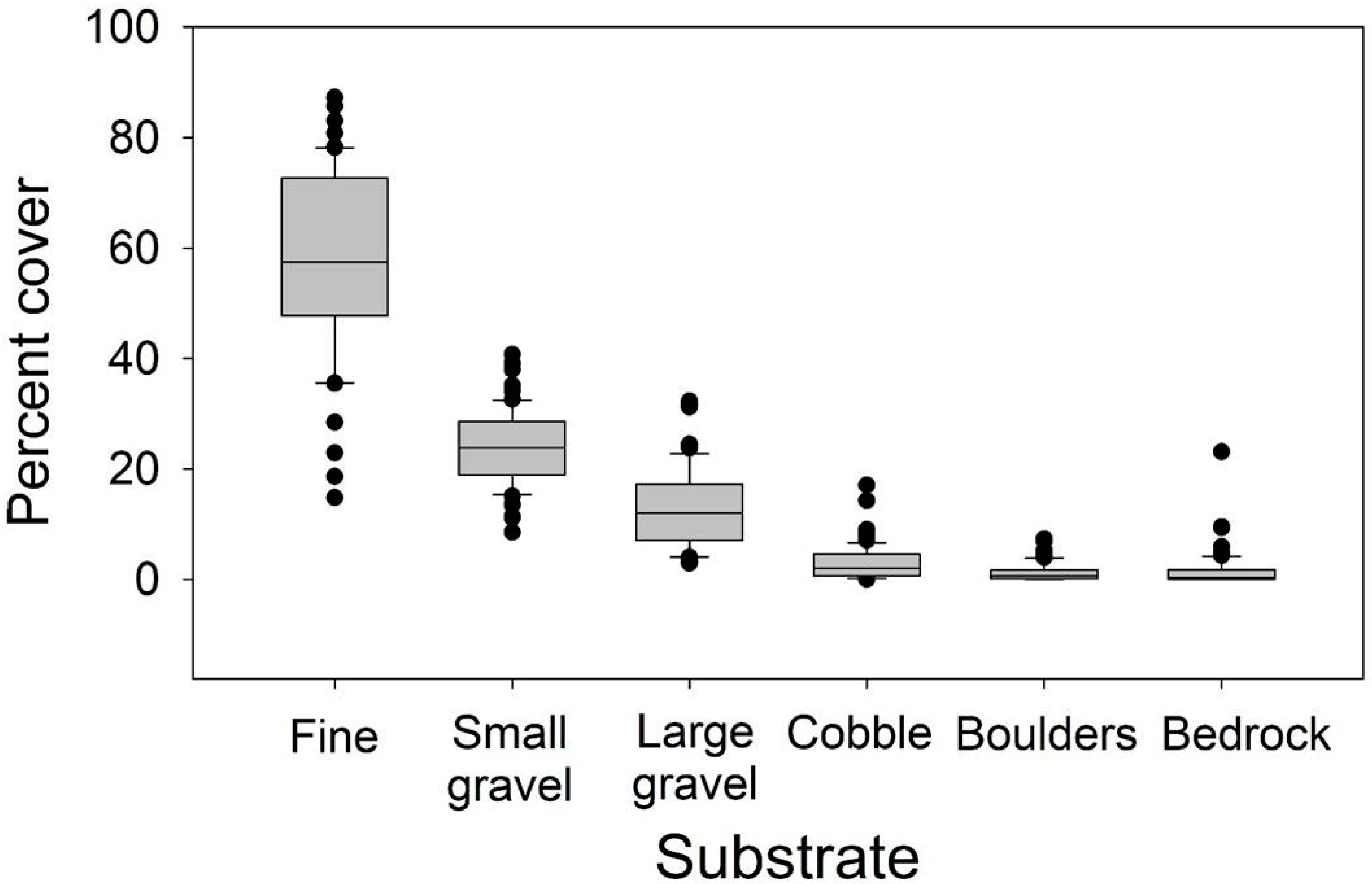
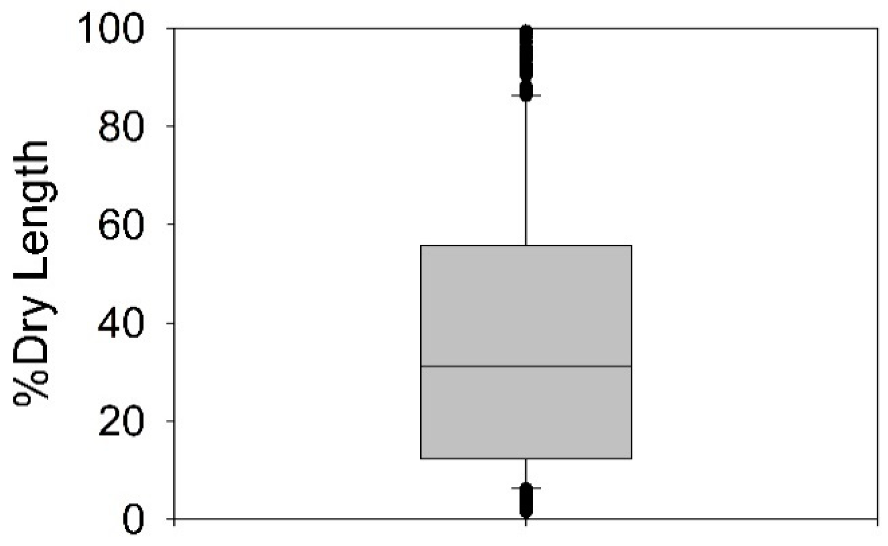
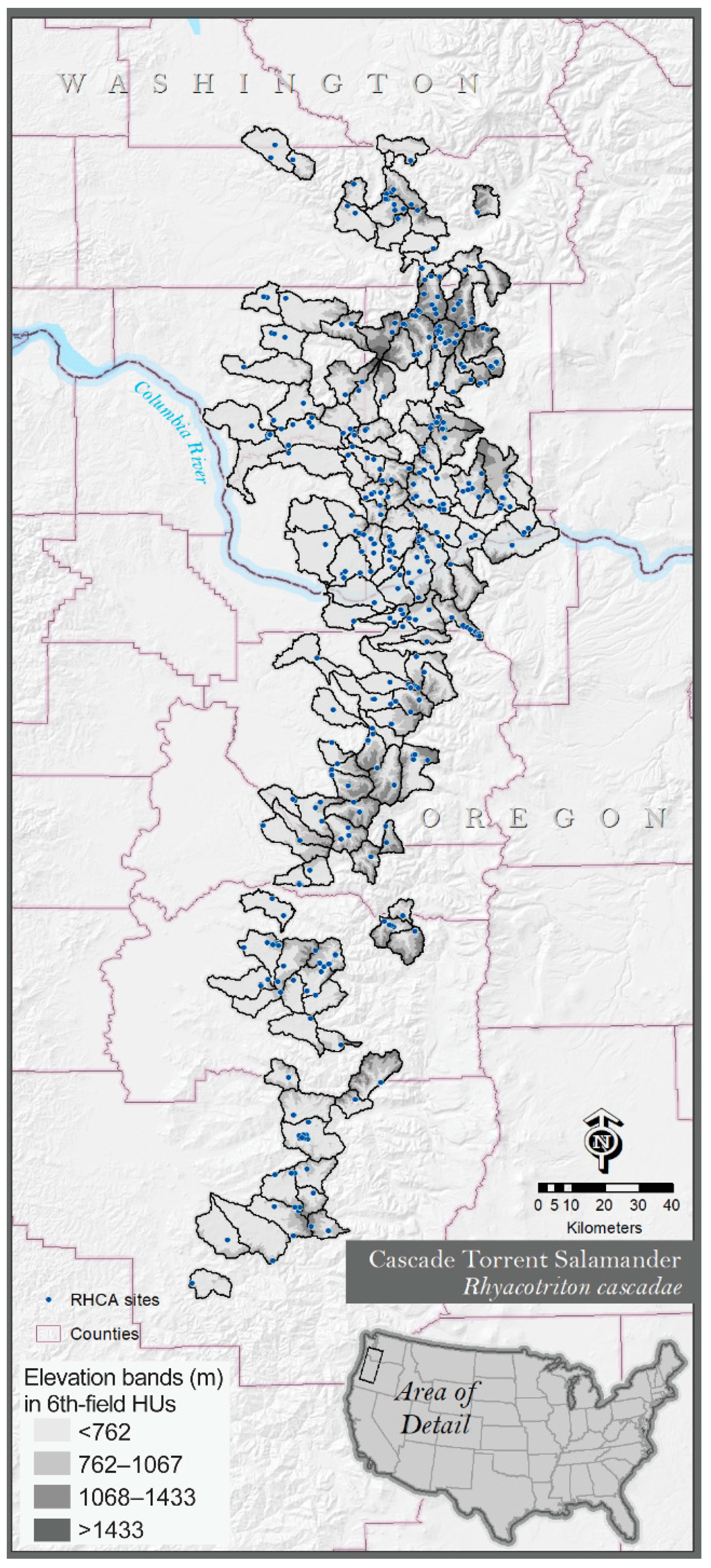
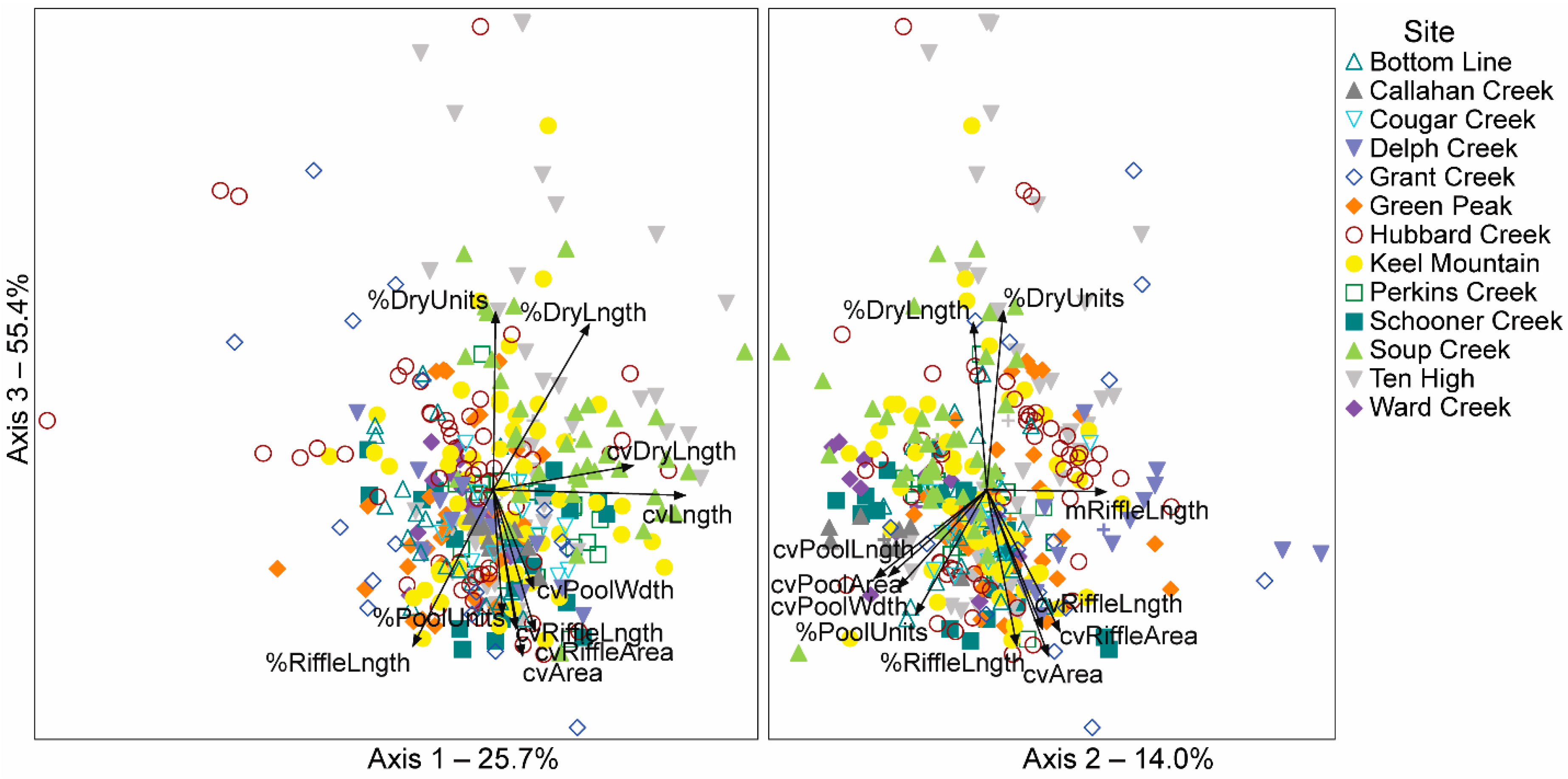
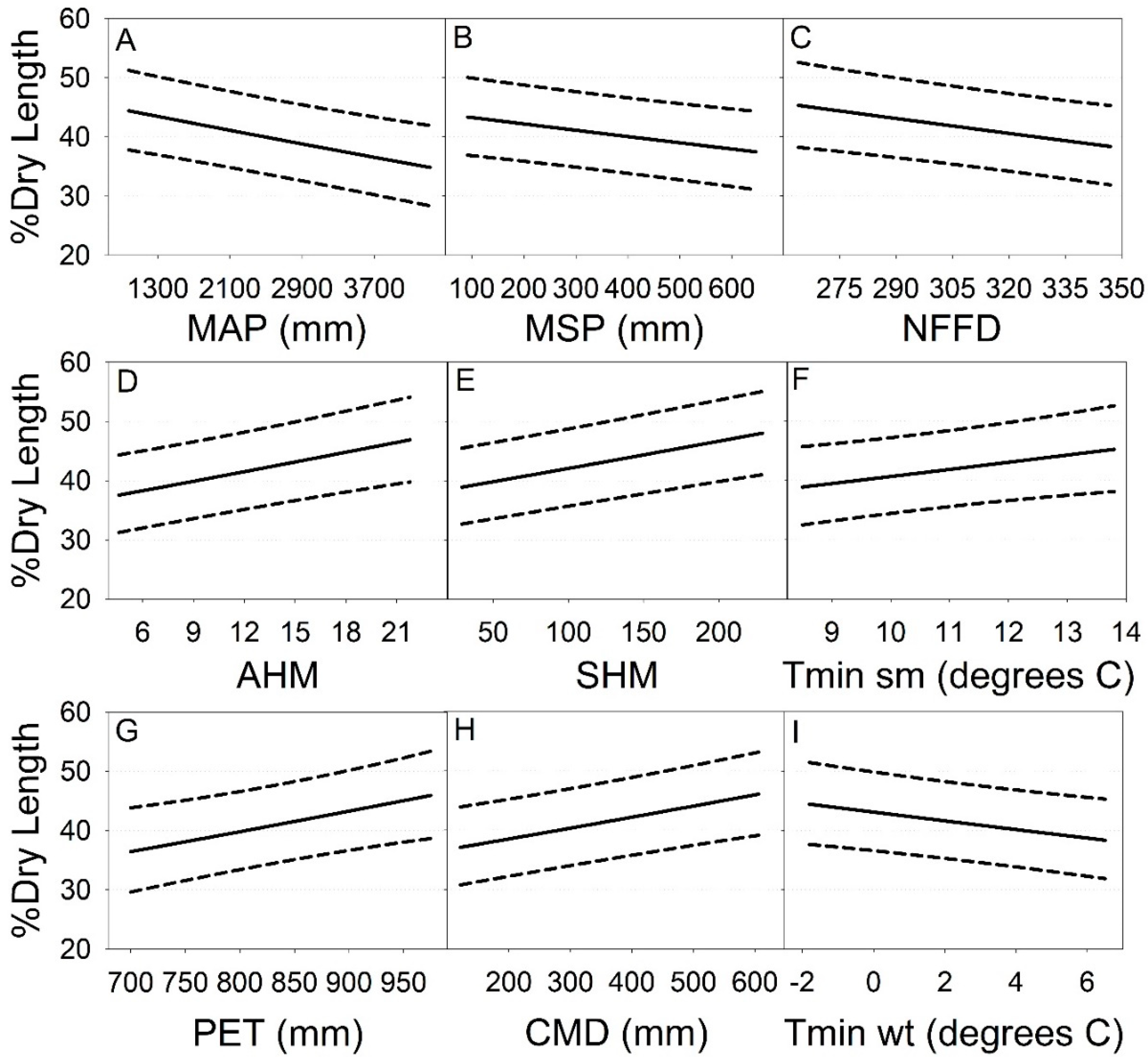
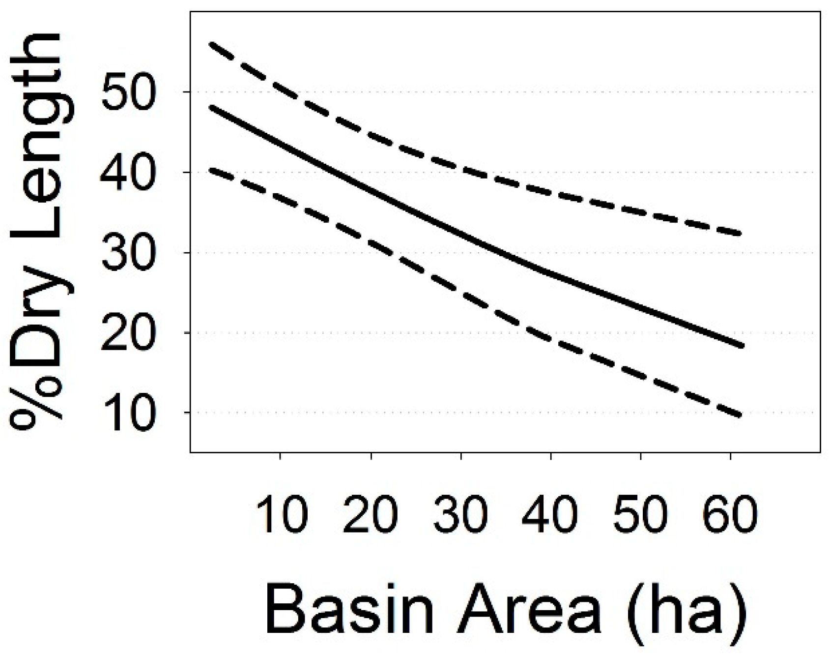
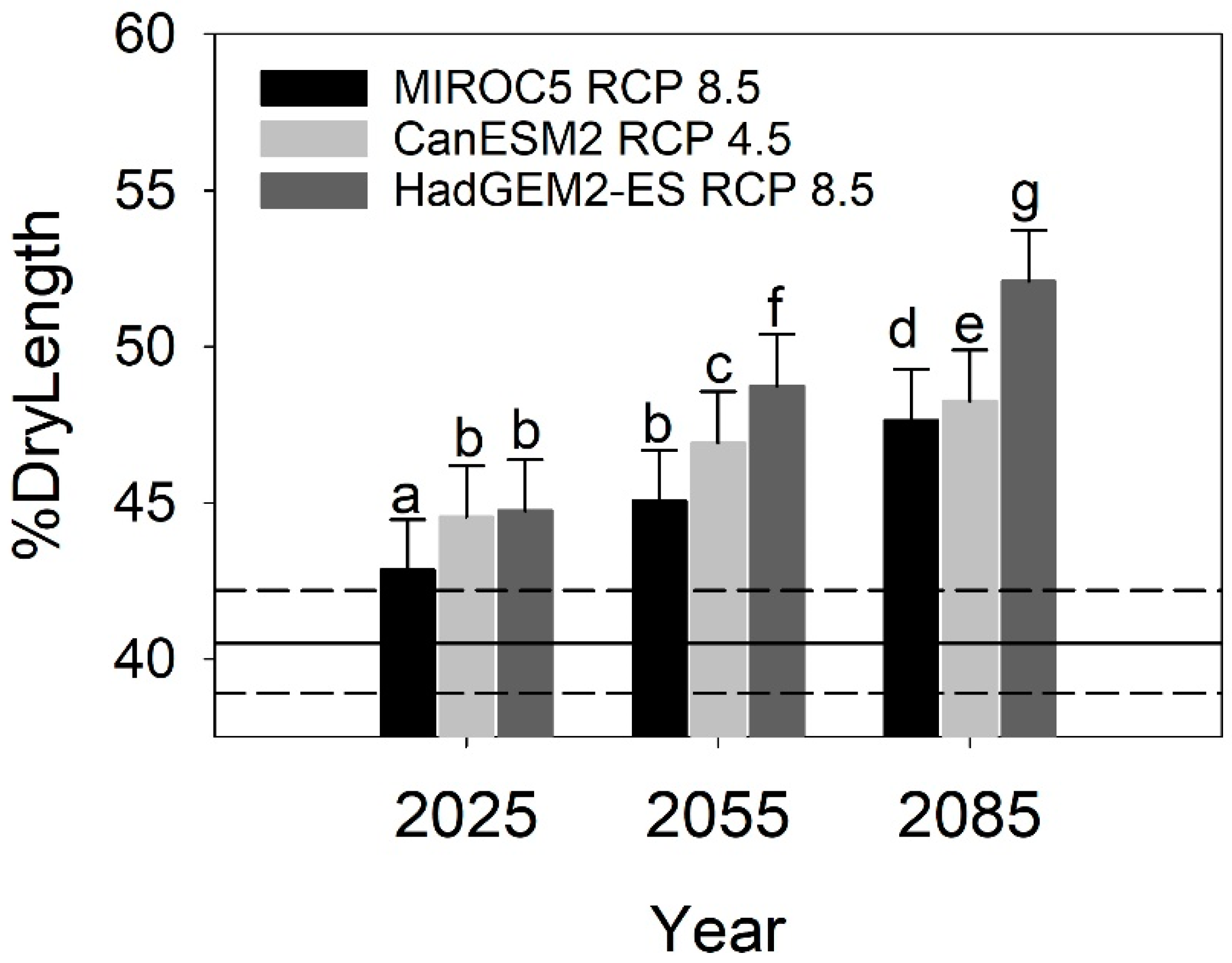
Table 1.
Number of spatially intermittent streams and stream reaches sampled by treatment category at each of 13 Density Management and Riparian Buffer Study sites in Western Oregon, USA. Reach treatment codes: 1 = one site-potential tree height riparian buffer, ~70 m; 2 = variable-width riparian buffer with a 15-m minimum width; 3 = streamside retention riparian buffer, ~6 m; 4 = control (no upland management during our study). Years sampled spanned 1995–2011 (but not 2007); reach numbers are indicated if there was subsampling in some years due to field logistical constraints. In the column Years Sampled, stream reach numbers within a site are provided if they were field-sampled during pretreatment surveys (indicated as year 0 in last column of table) and in post-treatment years 1–6, and 9–13.
| Site | No. Streams | No. Reaches | Reach Treatments | Years Sampled | Post-Treatment Year Sampled |
|---|---|---|---|---|---|
| Bottom Line | 6 | 7 | 1, 2, 4 | 1998, ′99, 2002 | 1, 2 and 5 |
| Callahan Creek | 1 | 1 | 3 | 1996, ′98, ′99, 2002, ′08, ′09, ′10, ′11 | 0, 1, 2, 5 |
| Cougar Creek | 2 | 3 | 2, 3, 4 | 1996, ′99, 2000, ′03 | 0, 1, 2, 5 |
| Delph Creek | 2 | 2 | 2, 3 | 2001, ′02, ′05, ′08, ′09, ′10, ′11, one also in 1997 | 0, 1, 2, 5, 8, 9, 10, 11 |
| Grant Creek | 3 | 4 | 2, 3, 4 | 1996, ’99, 2000, ′03 | 0, 1, 2, 5 |
| Green Peak | 4 | 4 | 2, 3, 4 | 1998, ′99, 2000, ′01, ′04, ′08, ′09, ′10, ′11 | 0, 1, 2, 5, 9, 10, 11, 12 |
| O.M. Hubbard | 6 | 9 | 1, 2, 4 | Reaches 34 & 36: 1995, ′98, ′99, 2002, ′08, ′09, ′10, ′11; reaches 28, 29, 31 & 32: 1995, ′98, ′99, 2002 | 0, 1, 2, 5, 11, 12, 13, 14 |
| Keel Mountain | 11 | 12 | 1, 2, 3, 4 | Reaches 41, 44, 54 & 56: 1995, ′99, 2000; reaches 153, 154, 158, 159 & 160: 2008, ′09, ′10, ′11; reaches 49, 51, 53: 1995, ′99, 2000, ′03, ′08, ′09, ′10, ′11 | Reaches 49, 51, 54, 56: 0, 1, 2; reach 53: 0, 1, 2, 10, 11, 12, 13; reaches 41, 44, 54, 56: 0, 1, 2; other reaches 10–13 |
| Perkins Creek | 3 | 3 | 3, 4 | 1997, 2000, ′01, ′04, ′08, ′09, ′10, ′11 | 0, 1, 2, 5, 9, 10, 11, 12 |
| Schooner Creek (1 & 2) | 3 | 3 | 2, 3, 4 | 1997, ′03, ′04, ′05/’06 | 0, 3, 4, 5/6 |
| Schooner Creek (5 & 6) | 3 | 3 | 2, 3, 4 | 1997, ′01, ′02, ′05 | 0, 1, 2, 5 |
| North Soup | 5 | 5 | 1, 2, 3, 4 | 1996, ′99, 2000, ′03, ′08, ′09, ′10, ′11 | 0, 1, 2, 5, 10, 11, 12, 13 |
| Ten High | 6 | 6 | 2, 3, 4 | 1997, 2001, ′02, ′05, ′08, ′09, ′11 | 0, 1, 2, 5, 8, 9, 11 |
| North Ward | 2 | 3 | 2, 3, 4 | 1997, 2005, ′08, ′09, ′10, ′11 | 0, 2, 3, 4, 5 |
Table 2.
Headwater stream reach and reach surface flow characteristics examined for 65 stream reaches sampled repeatedly from 1996–2011 in Western Oregon, USA. Average (standard error), minimum and maximum values are shown.
Table 2.
Headwater stream reach and reach surface flow characteristics examined for 65 stream reaches sampled repeatedly from 1996–2011 in Western Oregon, USA. Average (standard error), minimum and maximum values are shown.
| Stream Reach and Flow Characteristics | Average | Range | |
|---|---|---|---|
| Mean ± SE | Minimum | Maximum | |
| General reach characteristics | |||
| Dry to Wet ratio (Dry: Wet) | 2.6 (0.6) | 0.01 | 187.4 |
| Average | |||
| Unit length (m) | 14.7 (0.8) | 2.6 | 153.9 |
| Unit width (m) | 0.4 (0.01) | 0.1 | 2.1 |
| Unit area (m2) | 9.7 (1.6) | 0.05 | 312.2 |
| Variability | |||
| CV Unit length (%) | 155.8 (2.5) | 65.6 | 359.8 |
| CV Unit Width (%) | 45.8 (0.9) | 0 | 130.9 |
| CV Unit Area (%) | 140.1 (2.5) | 0 | 367.0 |
| % Units by major flow class | |||
| Dry | 30.9 (0.7) | 2 | 66.7 |
| Riffle | 43.7 (0.4) | 0 | 66.7 |
| Pool | 24.3 (0.8) | 0 | 54.5 |
| % Reach length by major flow class | |||
| Dry | 36.2 (1.4) | 1.5 | 99.5 |
| Riffle | 55.9 (1.4) | 0 | 96.7 |
| Pool | 5.8 (0.4) | 0 | 35.8 |
| Surface flow characteristics | |||
| Average | |||
| Length of dry units (m) | 18.3 (1.7) | 1.4 | 306.5 |
| Length of riffle units (m) | 15.9 (0.9) | 0 | 96.7 |
| Length of pool units (m) | 1.3 (0.05) | 0 | 9.4 |
| Width of riffle units (m) | 0.4 (0.01) | 0 | 2.1 |
| Width of pool units (m) | 0.4 (0.01) | 0 | 1.9 |
| Area of riffle units (m2) | 11.2 (1.6) | 0 | 420 |
| Area of pool units (m2) | |||
| Variability | |||
| CV Dry unit length | 107.3 (2.8) | 0 | 280.4 |
| CV Riffle unit length | 100.3 (1.9) | 0 | 221.8 |
| CV Pool unit length | 32.7 (1.4) | 0 | 180.3 |
| CV Riffle unit width | 44.5 (1.1) | 0 | 142.6 |
| CV Pool unit width | 28.2 (1.1) | 0 | 114.3 |
| CV Riffle unit area | 115.5 (2.3) | 0 | 286 |
| CV Pool unit area | 47.6 (2.0) | 0 | 364.9 |
| Climate Metrics |
|---|
| Mean annual temperature (°C, MAT) |
| Mean warmest month temperature (°C, MWMT) |
| Mean coldest month temperature (°C, MCMT) |
| Temperature difference between MWMT and MCMT, or continentality (°C, TD) |
| Hargreaves potential evaporation (mm, PET) |
| Hargreaves reference climatic moisture deficit (mm, CMD) |
| Degree days below 0 °C, chilling degree days (DD < 0) |
| Degree days above 5 °C, growing degree days (DD > 5) |
| Degree days above 18 °C, heating degree days (DD > 18) |
| Degree days below 18 °C, chilling degree days (DD < 18) |
| Number of frost-free days |
| Precipitation as snow (August in previous year—July in current year, in mm, PAS) |
| Mean annual precipitation (mm, MAP) |
| Winter mean maximum temperature (°C, Tmax wt) |
| Spring mean maximum temperature (°C, Tmax sp) |
| Summer mean maximum temperature (°C, Tmax sm) |
| Winter mean minimum temperature (°C, Tmin wt) |
| Spring mean minimum temperature (°C, Tmin sp) |
| Summer mean minimum temperature (°C, Tmin sm) |
| Annual heat: Moisture index ((MAT + 10)/(MAP/1000)) |
| Summer heat:moisture index (MWMT/(Mean Summer Precipitation/1000)) |
Table 4.
Pearson correlations between stream reach characteristics (average values unless otherwise indicated) and axes from non-metric multidimensional scaling ordination of 65 reaches (see Figure 5). sites measured repeatedly over time from 1995–2011 (Table 1). Correlation values (r) ≥ 0.11 are statistically significant (two-tailed test, p < 0.05). CV = coefficient of variation.
| Stream Reach and Flow Characteristics | Axis | ||
|---|---|---|---|
| Axis 1 | Axis 2 | Axis 3 | |
| General reach characteristics | |||
| Dry: Wet ratio | 0.279 | −0.106 | 0.353 |
| Unit length (m) | −0.067 | 0.467 | 0.49 |
| Unit width (m) | −0.324 | 0.268 | −0.251 |
| Unit area (m2) | −0.299 | 0.528 | −0.007 |
| Variability | |||
| CV Unit length (%) | 0.739 | 0.068 | −0.13 |
| CV Unit Width (%) | 0.134 | 0.325 | −0.157 |
| CV Unit Area (%) | 0.289 | 0.42 | −0.688 |
| % Units by major flow class | |||
| Dry | 0.079 | 0.217 | 0.71 |
| Riffle | −0.361 | 0.411 | −0.268 |
| Pool | 0.162 | −0.449 | −0.597 |
| % Reach length by flow class | |||
| Dry | 0.522 | −0.197 | 0.686 |
| Riffle | −0.477 | 0.29 | −0.667 |
| Pool | 0.088 | −0.476 | −0.437 |
| Surface flow characteristics | |||
| Length of dry units (m) | 0.309 | 0.193 | 0.368 |
| Length of riffle units (m) | −0.535 | 0.582 | −0.081 |
| Length of pool units (m) | −0.002 | −0.249 | −0.356 |
| Width of riffle units (m) | −0.296 | 0.312 | −0.279 |
| Width of pool units (m) | −0.08 | −0.198 | −0.485 |
| Area of riffle units (m2) | −0.278 | 0.521 | −0.112 |
| Area of pool units (m2) | −0.068 | −0.133 | −0.191 |
| Variability | |||
| CV Dry unit length | 0.63 | −0.12 | 0.262 |
| CV Riffle unit length | 0.252 | 0.396 | −0.629 |
| CV Pool unit length | 0.326 | −0.528 | −0.496 |
| CV Riffle unit width | 0.175 | 0.335 | −0.315 |
| CV Pool unit width | 0.339 | −0.502 | −0.529 |
| CV Riffle unit area | 0.345 | 0.456 | −0.634 |
| CV Pool unit area | 0.332 | −0.565 | −0.503 |
Table 5.
F-test results relating % dry length to annual and seasonal climate variables (Table 3) in simple linear models. Intercepts are not shown. All tests were based on 362 observations with one degree of freedom in the numerator. The response variable (% dry length) was transformed using a logit transformation prior to analysis.
| Variable | Estimate | SE | DF_Denom | F | p |
|---|---|---|---|---|---|
| MAT | −0.01134 | 0.02678 | 131 | 0.18 | 0.673 |
| MWMT | 0.03496 | 0.02047 | 215 | 2.92 | 0.089 |
| MCMT | −0.00817 | 0.01151 | 180 | 0.5 | 0.479 |
| TD | 0.01603 | 0.01041 | 249 | 2.37 | 0.125 |
| MAP | −0.00012 | 0.00003 | 128 | 13.24 | <0.001 |
| MSP | −0.00044 | 0.00016 | 101 | 8.16 | 0.005 |
| AHM | 0.02234 | 0.00594 | 109 | 14.15 | <0.001 |
| SHM | 0.00186 | 0.00036 | 57.5 | 26.57 | <0.001 |
| DD < 0 | 0.00082 | 0.00084 | 158 | 0.96 | 0.328 |
| DD > 5 | −0.00001 | 0.00009 | 132 | 0.02 | 0.881 |
| DD < 18 | 0.00004 | 0.00008 | 147 | 0.27 | 0.603 |
| DD > 18 | 0.00009 | 0.00038 | 136 | 0.06 | 0.813 |
| NFFD | −0.00344 | 0.00127 | 112 | 7.34 | 0.008 |
| PAS | −0.00164 | 0.00110 | 283 | 2.23 | 0.137 |
| Eref | 0.00143 | 0.00054 | 266 | 7.08 | 0.008 |
| CMD | 0.00077 | 0.00020 | 76.7 | 14.67 | <0.001 |
| Tmax wt | −0.02220 | 0.01445 | 75 | 2.36 | 0.129 |
| Tmax sp | 0.01336 | 0.01254 | 118 | 1.13 | 0.289 |
| Tmax sm | 0.01031 | 0.01668 | 200 | 0.38 | 0.537 |
| Tmin wt | −0.03033 | 0.01234 | 96.7 | 6.04 | 0.016 |
| Tmin sp | −0.01672 | 0.02089 | 161 | 0.64 | 0.425 |
| Tmin sm | 0.04943 | 0.02317 | 244 | 4.55 | 0.034 |
Table 6.
Final multivariate model relating the percentage of dry stream-reach length to basin area, summer heat:moisture index (SHM) and mean minimum summer temperature (Tmin sm). Conditional R2 = 0.82 and marginal R2 = 0.19.
Table 6.
Final multivariate model relating the percentage of dry stream-reach length to basin area, summer heat:moisture index (SHM) and mean minimum summer temperature (Tmin sm). Conditional R2 = 0.82 and marginal R2 = 0.19.
| Effect | Estimate | Standard Error | DF | t | Pr > |t| |
|---|---|---|---|---|---|
| Intercept | −0.812 | 0.209 | 147 | −2.80 | 0.0059 |
| Area (ha) | −0.024 | 0.007 | 38.7 | −3.26 | 0.0023 |
| SHM | 0.002 | <0.001 | 60.7 | 60.7 | <0.001 |
| Tmin sm | 0.058 | 0.022 | 250 | 2.63 | 0.0090 |
© 2019 by the authors. Licensee MDPI, Basel, Switzerland. This article is an open access article distributed under the terms and conditions of the Creative Commons Attribution (CC BY) license (http://creativecommons.org/licenses/by/4.0/).
Share and Cite
MDPI and ACS Style
Olson, D.H.; Burton, J.I. Climate Associations with Headwater Streamflow in Managed Forests over 16 Years and Projections of Future Dry Headwater Stream Channels. Forests 2019, 10, 968. https://doi.org/10.3390/f10110968
AMA Style
Olson DH, Burton JI. Climate Associations with Headwater Streamflow in Managed Forests over 16 Years and Projections of Future Dry Headwater Stream Channels. Forests. 2019; 10(11):968. https://doi.org/10.3390/f10110968
Chicago/Turabian StyleOlson, Deanna H., and Julia I. Burton. 2019. "Climate Associations with Headwater Streamflow in Managed Forests over 16 Years and Projections of Future Dry Headwater Stream Channels" Forests 10, no. 11: 968. https://doi.org/10.3390/f10110968
Note that from the first issue of 2016, this journal uses article numbers instead of page numbers. See further details here.