
Stochastic Flow Analysis for Optimization of the Operationality in Run-of-River Hydroelectric Plants in Mountain Areas

1
Fluvial Dynamics and Hydrology Research Group, Andalusian Institute for Earth System Research, University of Cordoba, 14071 Cordoba, Spain
2
Department of Mechanics, School of Engineering Science, University of Cordoba, 14071 Cordoba, Spain
3
Department of Agronomy, Unit of Excellence María de Maeztu (DAUCO), University of Cordoba, 14071 Cordoba, Spain
*
Authors to whom correspondence should be addressed.
Energies 2024, 17(7), 1705; https://doi.org/10.3390/en17071705
Submission received: 20 February 2024
/
Revised: 27 March 2024
/
Accepted: 29 March 2024
/
Published: 2 April 2024
(This article belongs to the Special Issue Climate Changes and the Impacts on Power and Energy Systems)
Abstract
:The highly temporal variability of the hydrological response in Mediterranean areas affects the operation of hydropower systems, especially in run-of-river (RoR) plants located in mountainous areas. Here, the water flow regime strongly determines failure, defined as no operating days due to inflows below the minimum operating flow. A Bayesian dynamics stochastic model was developed with statistical modeling of both rainfall as the forcing agent and water inflows to the plants as the dependent variable using two approaches—parametric adjustments and non-parametric methods. Failure frequency analysis and its related operationality, along with their uncertainty associated with different time scales, were performed through 250 Monte Carlo stochastic replications of a 20-year period of daily rainfall. Finally, a scenario analysis was performed, including the effects of 3 and 30 days of water storage in a plant loading chamber to minimize the plant’s dependence on the river’s flow. The approach was applied to a mini-hydropower RoR plant in Poqueira (Southern Spain), located in a semi-arid Mediterranean alpine area. The results reveal that the influence of snow had greater operationality in the spring months when snowmelt was outstanding, with a 25% probability of having fewer than 2 days of failure in May and April, as opposed to 12 days in the winter months. Moreover, the effect of water storage was greater between June and November, when rainfall events are scarce, and snowmelt has almost finished with operationality levels of 0.04–0.74 for 15 days of failure without storage, which increased to 0.1–0.87 with 3 days of storage. The methodology proposed constitutes a simple and useful tool to assess uncertainty in the operationality of RoR plants in Mediterranean mountainous areas where rainfall constitutes the main source of uncertainty in river flows.
1. Introduction
Hydropower is one of the cheapest renewable energy sources that can be generated without toxic waste [1,2] and has very low operation and maintenance costs [2,3]. Of the total renewable energy production in Europe, the majority was generated from hydropower, accounting for 425.8 TWh [4]. Most hydropower plants in use today are traditional or conventional hydropower plants designed with a dam, a lake, a penstock, and a powerhouse. In contrast, non-conventional hydropower plants, such as run-of-river (RoR) power plants, constitute a more environmentally friendly option [1,2,5]. In RoR plants, a fraction of the stream flow is diverted through penstocks to a powerhouse and then returned to the stream. The reservoir is frequently absent, or it is a tiny pond or chamber.
The contribution of small hydropower plants (SHPs) to the worldwide electrical capacity is at a more similar scale to the other renewable energy sources (1–2% of the total capacity) [3]. Europe is the market leader in small-scale hydropower technology, with Spain, Italy, France, Germany, and Sweden being the main producers [3]. Small SHPs and, among them, RoR plants are especially useful thanks to their low administrative and executive costs and short construction time compared to projects with storage reservoirs of a similar power capacity [5].
The operation of hydroelectric power plants is subject to different conditioning factors, including the hydraulic conditions of the riverbed, the specific operating conditions of the plant’s instrumentation, and certain restrictions, such as compliance with the environmental flow regime established in the corresponding legislation. One of the main drawbacks of RoR plants is the high degree of uncertainty of the available river flows upstream of the plant owing to meteorological fluctuations, resulting in an unpredictable power generation capacity [5,6], which is even more prevalent in the current climate change scenario [2,7,8].
Some of the main energy infrastructures affected by climate change are hydropower plants located in snow-covered mountainous areas, where climate change is expected to result in a later and shorter snow season and less snow coverage [8,9]. Mountains are considered “water towers” since they provide water for both ecosystems and anthropogenic demands in downstream areas [10]. In Mediterranean mountains with both alpine and semi-arid conditions, the variability in the climate enhances the complexity of the hydrological regime. These areas have particularly extreme conditions, in which the high variability in the annual and seasonal climate regimes is usually propagated and amplified by the river flow [10]. Moreover, the highly variable snowpacks, in both time and space, and the presence of several accumulation and melting cycles during the snow season lead to a strong seasonality of the streamflow response in headwater catchments [11]. Thus, RoR plants in Mediterranean mountains operate with even more irregular production subject to the run-of-river flow, which depends on the highly variable forcing agents of the rainfall–runoff processes and snow cover dynamics. Consequently, these plants often have to cease operation when the flow drops below the turbine operating level or rises above the maximum allowed by the turbines, thus affecting power generation and, therefore, plant performance [2].
RoR systems are subject to several uncertainties in both operation and management [12]. Thus, the challenge of the operation of RoR hydroelectric plants for water resource managers is to quantify how much water will be available for power generation. Especially in the Mediterranean snow-dominated mountains where river flows follow a strong seasonal pattern with significant interannual variability, having a seasonal forecasting system with limited uncertainty and sufficient reliability for decision-making would be a very useful tool for their seasonal and annual planning and would reduce opportunity costs due to the lack of such a forecast.
Thus, the main objective of this study was to obtain a simple and versatile stochastic flow-forecasting structure from the significant forcing agents that allow for anticipating the regime of river inflows to run-of-river hydroelectric power plants and the number of days of failure for operational purposes at time scales of interest in hydrological planning. In addition, the effect of possible storage in a load chamber was included to optimize the operation of the chamber by minimizing the run-of-river power plant’s dependence on the river flow. The most critical component of river flows in Mediterranean areas are low flow periods because of the mild winter temperatures in combination with long, dry, sunny periods [13]. Thus, the minimum regime as the most limiting variable in the operation of power plants constitutes the basis of this study.
Stochastic models are often applied in hydrology to generate different samples of meteorological and hydrological data that are equally likely with respect to the observed series [14,15]. The stochastic forecasting structure developed in this study is based on scientific knowledge of rainfall–runoff processes and a rigorous analysis of the stochastic relationships of their main descriptor variables. Therefore, the main forcing agents that determine the increase in humidity in the contributing basin were first identified. Secondly, an analysis was carried out to identify the significant relationships between the forcing agents and the target variables at the different temporal scales established. Then, a Bayesian analysis of the probability of occurrence of the inflow rates was made based on the antecedent hydrological conditions. Finally, a scenario analysis was performed to assess the effect of using a small storage chamber to optimize the management of hydroelectric power RoR plants with maximum use of the natural fluvial contributions in the study area.
2. Materials and Methods
2.1. Study Site and Data Sources
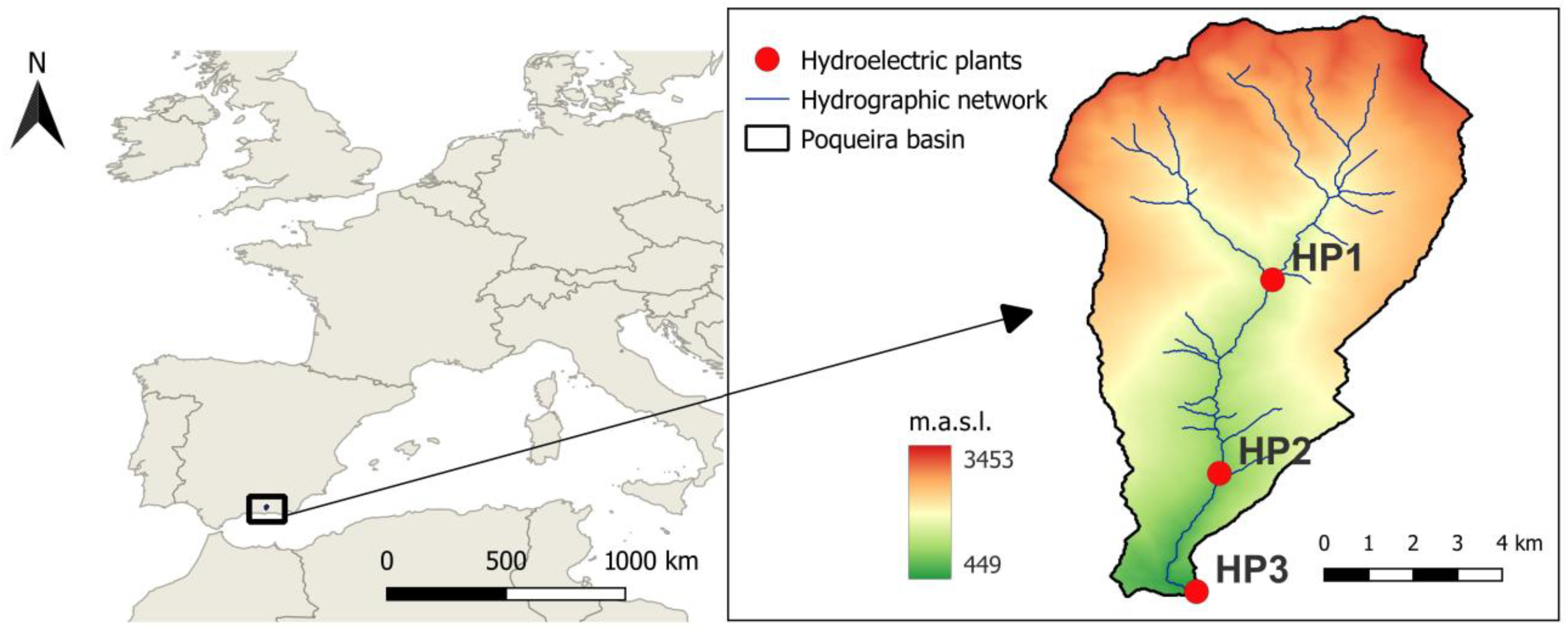
The study site was the Poqueira system in Sierra Nevada (37° N; −3.3° W), which is a national park and biosphere reserve located in a mountainous area in southern Spain, where the presence of snow has a great effect on the hydrology of the downstream areas [8]. The contributing basin to the hydropower plants has an area of 38.4 km2, with an average slope of 23° and an elevation ranging from 3453 m a.s.l. to 449 m a.s.l., with a mean value of 2161 m a.s.l. There is great variability in the precipitation regime due to the interaction of both the alpine and Mediterranean climates of the region, with the accumulated annual precipitation rate reaching 1200 mm in wet years and 220 mm in dry years within the period of 1961–2015 [2]. Above 2500 m a.s.l., the presence of snow is persistent, although it is commonly found at altitudes above 1000 m a.s.l. from November to May, with a very heterogeneous spatial distribution of the snow cover [2,11].
Three consecutive RoR hydroelectric plants, HP1, HP2, and HP3 (Figure 1), belonging to an important Spanish company in the energy sector and with a capacity between 10 and 12 MW, are located in the basin [2]. The hydroelectric plant located at the highest altitude is Poqueira (HP1), which is supplied from a load chamber located at 2100 m a.s.l. The operation of this system is as follows: the turbined flow in the upstream plant (HP1) is carried through a pipeline that connects the load chambers to the next plant (HP2). In the same way, from the latter, it reaches the HP3 plant. For the study of the operation of these mini power plants in a concatenated series, only the case of HP1 has been analyzed since the turbine flow in this plant determines the operation of the other two plants downstream. For this reason, ecological flow restrictions must be applied to the HP1 plant since it is the first one in the series. The minimum ecological flow established in the Basin Hydrological Plan to be supplied from the HP1 plant is 0.35 m3/s, as a constant flow throughout the year [2]. Therefore, the minimum operating flow of HP1 is the sum of the minimum turbine flow and the minimum ecological flow established (Table 1).
This hydroelectric power plant has a low-capacity load chamber that can be used to slightly compensate for the effect of a significant decrease in the inflow to the plant. Its low storage capacity means that it can be considered a RoR plant.
Regarding meteorology, the available daily data (precipitation, temperature, solar radiation, humidity, and windspeed) belong to different meteorological networks in the area (Red Guadalfeo, SAIH Guadalquivir, RIA-JA) [2,16,17,18]. Daily flow series at the basin outlet are available from the SAIH (automatic hydrological information system) of the Andalusian internal basins between 1998 and 2015.
For the hydrological characterization of the contributing basin to HP1, a series of hydrometeorological data of sufficient length were required to collect different scenarios of extreme flow events, both dry periods and floods, as well as periods of average flow in the basin. In general, data series of at least 20 years are required to obtain meaningful estimations from fluvial regimes in which periodicities in flow have an important bearing [19,20]. Given that the available data series have some gaps and due to the need to use cumulative values distributed over the contributing basin to the HP1 hydroelectric power plant, a hydrological simulation was carried out in the basin for the period from December 1998 to August 2019 with the WiMMed (Water Integrated Management in Mediterranean Environments) model, a physically based and fully distributed hydrological model [21]. The use of the WiMMed model is justified as it was conceived considering the particularities that exist in Mediterranean areas in terms of the large spatial and temporal variability in the variables and parameters that determine the rainfall–runoff processes, with special consideration of drying processes. In fact, the WiMMed model is already calibrated and validated in numerous Mediterranean basins [22]. The WiMMed model performs hourly calculations of the energy and water balance on a gridded representation of the terrain, providing input data to circulate both the surface and sub-surface flows throughout the basin area to the selected outlets.
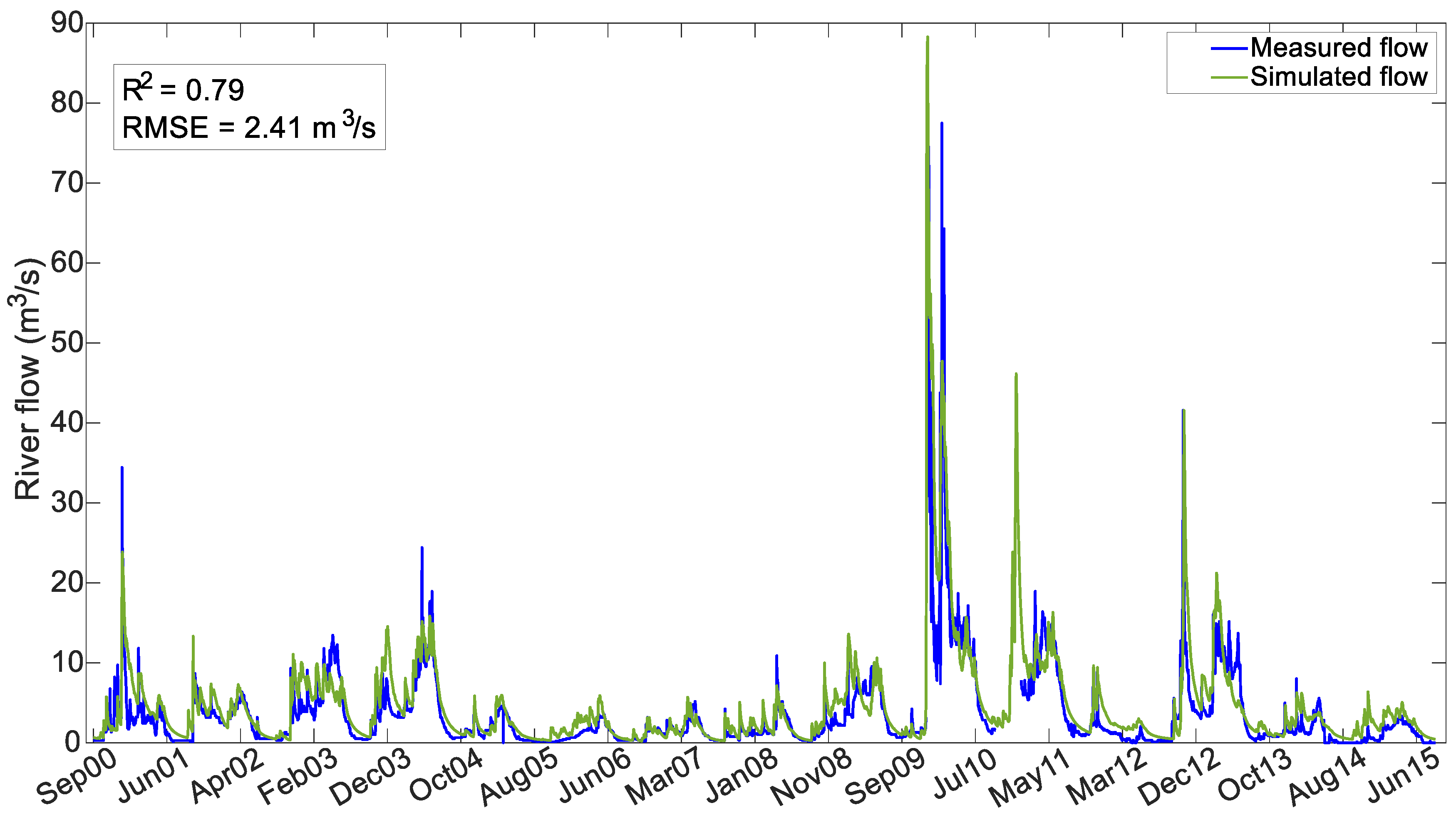
In previous studies [13,21,23], the model was calibrated in the contributing basin where the headwater watershed that contributes to HP1 is located. The accuracy of distributed precipitation estimation is one of the most significant factors when reproducing the fluvial regime in semiarid regions [13,24,25]. More information regarding the datasets used to implement the model on the study site can be found in the literature [2,13,16,21,23]. The results of the hydrological simulation and the measured flows in the period from 1998 to 2015 with available measurements are shown in Figure 2. The correlation coefficient between the daily series of measured and simulated flows is 0.79, so it is considered that the simulation correctly represents the hydrological dynamics of the basin.
Following the hydrological simulation performed using the WiMMed model, daily maps with a 30 × 30 m cell size resolution were generated for rainfall, snowfall, snow water equivalent, snowmelt, and evaposublimation. Table 2 presents the mean, maximum, minimum, and standard deviation values of the mean daily river flow (Q), accumulated rainfall (R), snow water equivalent (SWE), and snowmelt (SWM) in the contributing basin to the HP1 power plant at the annual and monthly scales. The mean spatial annual values were computed as the aggregation of the daily values for each water year (from September to August for the latitude of the study site). The strong hydrological variability typically found in semiarid Mediterranean mountainous areas [13,26] can be appreciated at the study site, where there are monthly maximum flow values (Q) of up to 4.8 m3/s in January and 0.59 m3/s in August. The interannual variability is also evident, with extreme values (maximum and minimum) that sometimes exceed by one order of magnitude the mean values of most of the variables.
2.2. Methodological Framework
In order to carry out the stochastic analysis, first the dependency structure between the forcing agents and the objective variables related to plant operationality was obtained at the annual and monthly scales to select the most influential forcing variables. Then, a Bayesian dynamics forecast of the water inflows to the plant was computed with the application of the Monte Carlo technique together with statistical modeling of the objective variables using two approaches—parametric adjustments and non-parametric methods. Parametric methods refer to the parametric relationships between the forcing agents and the target variables, such as polynomials, exponentials, or potential adjustments. In contrast, non-parametric methods assume that the data do not have a particular statistical distribution and, thus, are based on the use of the empirical cumulative distribution functions of the variables. Using the probability distribution functions of inflows to the plant and the variable number of days of failure at the corresponding time scale, the probability of the plant’s operationality was then computed.
Finally, an assessment of the operationality of the hydropower plant was performed with the analysis of several scenarios, including the hydropower plant operation rules and varying levels of water stored in the loading chamber.
2.2.1. Dependency Structure among Variables
First, the forcing agents and target variables were identified at the annual and monthly scales since these are the time scales of interest in the operation of hydroelectric power plants. Forcing agents are the variables that determine the increase in humidity in the basin that supplies the hydroelectric plants. Since this is an area influenced by a high mountain climate, in addition to rainfall, the presence of snow strongly determines the hydrological dynamics of the contributing basin [11,16]. Therefore, rainfall, snowfall, snow water equivalent, snowmelt, and evaposublimation were identified as possible forcing agents for the dependence analysis.
In terms of target variables, operationality has been defined in the scope of this study as the probability of being able to produce energy in the hydroelectric plant in 20 years. Operationality is, therefore, the complement of the probability of failure [13], with failure being defined as the day on which there is no energy production due to the flow being lower than the minimum operating flow. Therefore, the number of days on which the plant did not operate due to a circulating flow lower than the minimum operating flow was generated from the data series of daily flows available. The relationship between the two variables was then analyzed in order to quantify the probability of failure based on the mean daily flow. Thus, the final target variables are the mean daily flow (Qmean) and the number of days of failure (Nfailure) at the annual and monthly scales.
Based on the 20-year series of the variables considered, classical descriptive analysis techniques were applied by means of adjustments and analysis of the correlation coefficients between the series of forcing agents and target variables at different time scales—annual and monthly. The adjustments made between the variables were parametric relationships of the first-, second-, and third-degree polynomials, exponentials, and potentials. Due to space limitations in the Results section, only the best correlations obtained from all the parametric adjustments made for each variable are shown. However, all the parametric fits can be made available upon request to the authors.
Finally, the best parametric adjustments obtained for each time scale were selected.
2.2.2. Bayesian Dynamics Forecast of Water Inputs and Analysis of Operationality
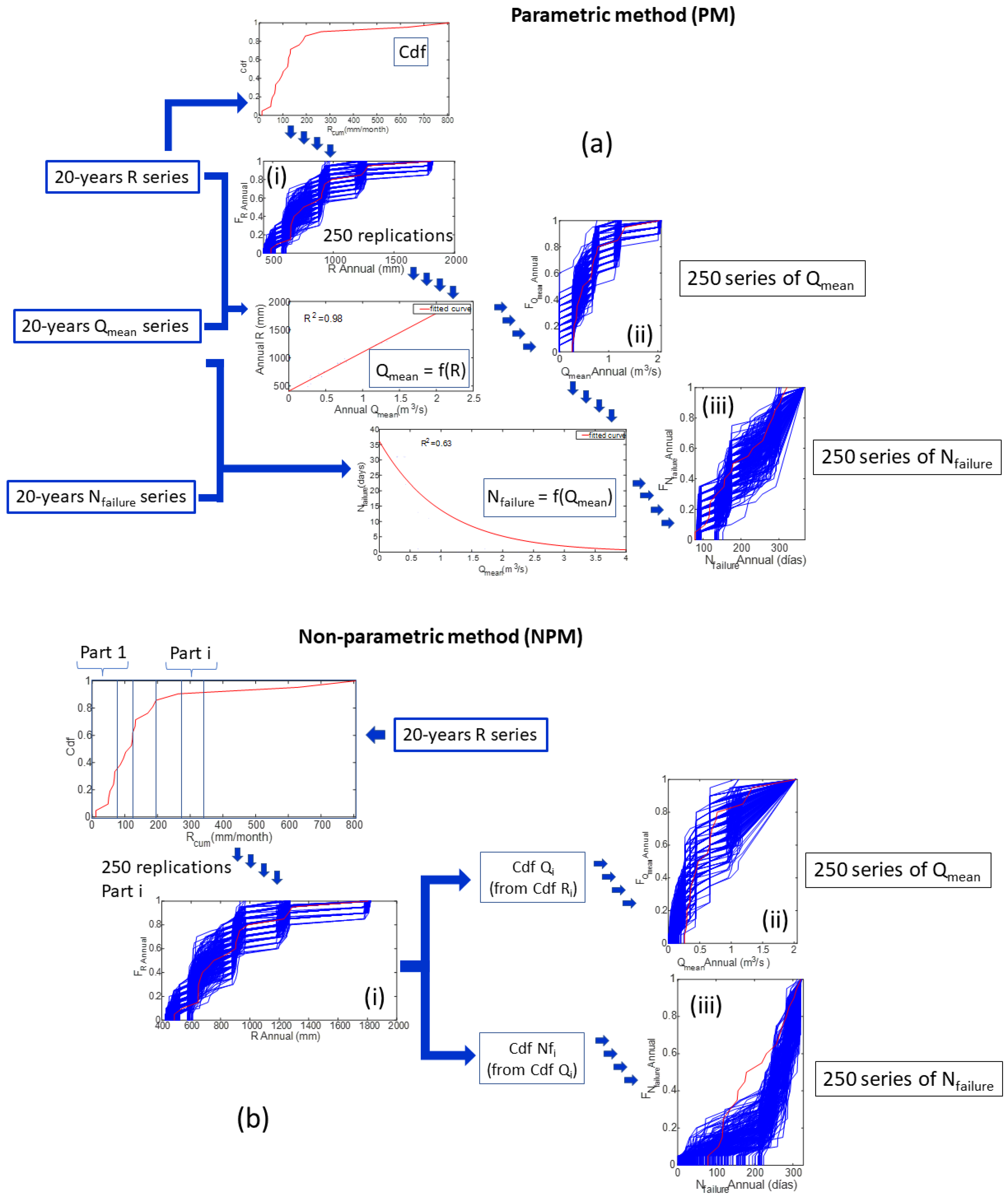
In order to generate predictions of the target variables, the mean daily flow, and the number of days of failure, along with their associated uncertainty, the simulation of the forcing agent by Monte Carlo was combined with two approaches or methods—parametric and non-parametric. Figure 3 shows the calculation sequence with rainfall (R) as the forcing agent.
The parametric method (PM) is based on the parametric relationship between the forcing agent (e.g., rainfall or snowfall) and the target variable generated in the previous section. This method starts with the cumulative distribution function (cdf) of the forcing agent accumulated at the corresponding time scale and continues with the following calculation sequence, which shows rainfall as an example of the forcing agent (Figure 3):
- A total of 250 sets of 20-year series of equally probable rainfall were obtained with Monte Carlo using the cdf of the available rainfall data series.
- The mean daily flow was calculated from the best parametric fit with the accumulated rainfall; thus, the forecast was included in the calculation.
- The number of days of failure was calculated from its best parametric relationship with the mean daily flow (Appendix A).
Regarding the non-parametric method (NPM), techniques already used in various areas of Europe were applied [13,22]. In this case, we started directly from the cumulative distribution functions of the rainfall, the mean daily flow, and the number of days of failure at the annual and monthly scales. Each of these functions was divided into 6 parts, considering the criterion that in each of these sections there should be at least 3 data points of the average flow or number of days of failure. Then, the cdf of each of the partitions of the different cumulative distribution functions was developed. Based on these developments, the calculation sequence of the non-parametric method was as follows (Figure 3):
- A total of 250 sets of 20-year series of equally probable monthly rainfall were obtained with Monte Carlo using the distribution of the available monthly rainfall data series.
- The obtained rainfall values were used to generate 250 repetitions of the 20-year mean daily flow data series, applying quantile mapping to the distribution functions generated in the partitions of the distribution functions of the measured data series, as this procedure is analogous to generating 250 repetitions of a series of number of days of failure.
Finally, the operationality of the hydropower plants was analyzed in terms of the complementary probability associated with the occurrence of failure based on the flow regime. To accomplish this analysis, the cdf of the target variables (the mean daily flow and the number of days of failure at the annual and monthly scales) was intercepted at the y-axis at the corresponding quartiles of 1, 2, and 3. Thus, it is possible to know with a 25, 50, or 75% probability whether the number of days of failure per year or month does not exceed a certain value above which the production of hydroelectric energy becomes unfeasible.
2.2.3. Scenario Analysis
Once the forecast of the number of days of failure for a given month is known, it is useful to know the effect of possible storage in a small load chamber to maximize the use of the incoming natural fluvial contributions.
The variable that determines the failure in the operation of a plant is a mean daily flow lower than the minimum daily operation flow, assigning to the variable Nfailure the failure or not in the operation of the plant. Scenario analysis was performed with a variable storage volume, which was null in case it did not exist, in order to simulate the operation of the plant as a pure RoR plant.
The number of days of failure was calculated on a daily scale from the available flow data series. Thus, the variable Nfailure was assigned the value of failure or not, not only depending on the availability of the flow provided but also taking into account the volume stored in the load chamber, if any. Then, the number of days of failure as a measure of operationality was aggregated at the corresponding time scale. Three were analyzed: no storage in the load chamber, which is equivalent to pure RoR plants, and a small load chamber volume equivalent to 3 days, which is the capacity of the chambers in other RoR plants in the area with similar characteristics (i.e., power generation capacity). Also, for comparison with traditional hydropower plants with larger storage systems, a chamber volume equivalent to 30 days is shown. This last value, oversized for the characteristics of the plant under study, is shown only for visual effect in order to clearly elucidate the effect of storage.
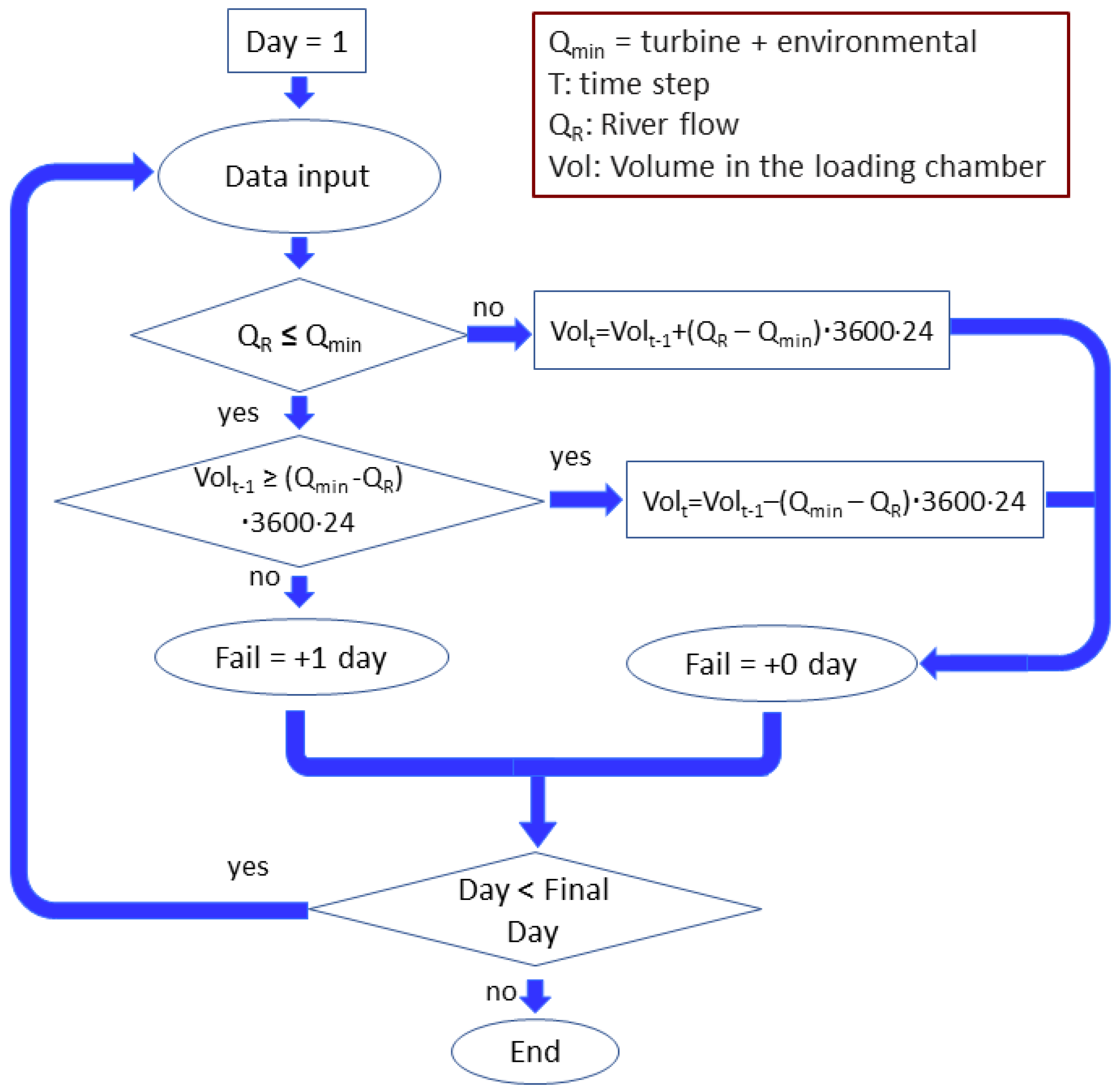
Figure 4 shows the flow chart of the plant operation calculation:
- 1.
- It is checked whether the incoming flow is equal to or higher than the minimum turbined flow to operate the plant.
- If it is equal to or higher, a new volume of available water in the water chamber is calculated, which is equal to the existing volume plus that which exceeds the incoming flow on the day after the release. The day is assigned as a non-failure in the operation of the plant.
- If it is lower or null, it is checked to see whether the incoming flow can be supplemented with the stored volume available in the load chamber.
- -
- If it can be supplemented, the new volume of the load chamber is calculated after extracting the required volume. The day is assigned as a non-failure in the plant’s operation.
- -
- If it cannot be supplemented, the day is assigned as a failure in the plant’s operation.
- 2.
- The calculation continues until the 20-year series is complete.
Figure 4.
Flux diagram of the scenario analysis from the calculation of Nfailure for hydropower plant management.
Figure 4.
Flux diagram of the scenario analysis from the calculation of Nfailure for hydropower plant management.

3. Results and Discussion
3.1. Dependency Structure between Variables
3.1.1. Annual Scale
At an annual scale, a good linear relationship was observed between the maximum annual daily flow (Qmax) and the mean annual daily flow (Qmean) (Table 3), with an R2 value of 0.82. Regarding the relationship of the maximum annual daily flow with the average annual rainfall (R) and maximum annual daily rainfall (Rmax), lower linear correlations were observed, with R2 values of 0.8 and 0.52, respectively. The low correlation in this latter analysis can be explained by the snow influence in the area, which determined that the day with the maximum daily flow was not the same as the day with the maximum daily rainfall.
The best correlations at the annual scale were found between the annual mean daily flow and the average annual rainfall (R), reaching an R2 of 0.98, and the average rainfall minus the evaposublimation flux (R − ES) (Table 3), since it represents the net precipitation that directly contributes to runoff generation. Regarding the correlation between the annual mean daily flow and the snow-related variables, average snowfall (S), average snow water equivalent (SWE), and average snowmelt (SWM), slightly lower linear correlation coefficients were obtained. oscillating between 0.67 and 0.75, with the highest correlation being with snowmelt (0.75). These lower values were due to the highly variable snowpack with the presence of several accumulation and melting cycles during the snow season, as well as a non-negligible evaposublimation flux [11].
Regarding the annual number of days of failure (Nfailure), the best correlations were found with both the mean annual daily flow and the annual rainfall, obtaining R2 values of 0.63 and 0.65, respectively.
3.1.2. Monthly Scale
At a monthly scale, not only the linear correlation was considered but also the quadratic and exponential correlation, following previous studies that have flow-related variables [27,28] and use rainfall as the independent variable to better capture the non-linear effects of the hydrological water balance at shorter time scales. In addition, correlation with the value of some variables in the antecedent month was included in the analysis in order to analyze a possible monthly lag effect in the circulating flow.
Table 4 shows the correlation coefficients obtained between the monthly mean daily flow variable and the rest of the variables identified at a monthly scale for the best adjustments obtained for the sake of greater conciseness of the manuscript. However, the values obtained for all the adjustments per month carried out in this study can be made available upon request to the authors.
Analogously to the annual scale, a good correlation was again observed between the maximum monthly daily flow and the mean monthly flow, with R2 values between 0.74 and 1 (Table 4).
Regarding the monthly rainfall (Rm), good correlations were observed in the months of October, January, February, March, and July, with correlation coefficients between 0.65 and 0.84. When the same analysis was performed with the rainfall in the previous month (Rm_prev), the highest correlation coefficients were found in January, February, April, and November, with even higher R2 values between 0.72 and 0.92.
As for the monthly snowfall (Sm), there was a good correlation only in the month of February (0.76, Table 4), reaching higher values in the months of November, January, March, and April with the snowfall of the previous month (Sm_prev). Finally, with respect to the monthly snow water equivalent (SWEm) and the snowmelt (SWMm), the correlation coefficient values were higher than 0.51 in the months from January to July, exceeding 0.62 in most months (Table 4).
At the monthly scale, the correlation between the monthly number of days of failure (Nfailure) and the monthly mean river flow (Qm mean) reached R2 values of over 0.77 in most months (Table 4), exceeding 0.86 in most cases. Thus, the number of days of failure can be reproduced once the required forecasts of monthly river flows are available.
As already pointed out by previous studies at the study site [11], the peculiar snow dynamics result in the seasonality of the streamflow response in this headwater catchment. These results confirm this statement as the highest correlations with respect to the mean monthly flow occurred in the winter months, with monthly rainfall improving, in some cases, the correlation with respect to the rainfall of the previous month. In contrast, in the spring and summer months, the best correlations were obtained with the snowmelt and snow water equivalent. Despite being clear that the precipitation and snow depths impacted the monthly river flow, their effect was not instantaneous. Thus, this non-instantaneous time relationship needs to be considered, as already applied in previous studies [29], when looking for the best forcing variable at the monthly scale.
Considering that the main source of uncertainty in the flow regime in Mediterranean watersheds is due to variability in the occurrence of meteorological agents (mainly rainfall) [30], a more detailed analysis of lag times in the influence of rainfall accumulated in the antecedent months on the river flows was carried out. This analysis helped to solve the low correlation values obtained between the monthly mean flow and the monthly rainfall (Table 4) in certain months (e.g., December, May, and June). Thus, Table 5 shows the best correlations found for the monthly mean flow with one or several antecedent months of accumulated rainfall, as appropriate. The correlation coefficients in the table refer to the first-, second-, and third-degree polynomial adjustments, exponential adjustments, and potential adjustments in the case of December. The parametric expressions of these adjustments can be found in Table A1 in Appendix A. Correlation coefficients higher than 0.7 were reached in all months, and thus, these adjustments were used to reproduce the monthly river flow dynamics once the required forecasts of monthly rainfall were available. It can also be observed how, in most months, better correlations were obtained than those resulting from considering the current month or only a lag of one month (Table 4). The only exception is September, when no good correlation was found, neither with the rainfall in September nor extending the analysis to the rainfall of previous periods accumulated at various time scales, which is in accordance with previous studies in the basin encompassing the study area [13].
Two trends can be observed that group the forecast into three blocks. From October to December, the highest correlation was obtained between the rainfall of the previous month and that of the current month, i.e., the October flow was obtained with the accumulated rainfall of September and October, and in the same way, with November and December. In these months, the flow was mainly produced directly by the occurrence of rainfall–runoff events, mainly in liquid form, which explains this correlation between the previous month and the current month.
In the months of January and February, the occurrence of solid rainfall events or snowfall begins to be more frequent, so water accumulates in the snow layer and the proportion of direct runoff decreases, introducing a certain lag time in terms of river flows. Therefore, it was observed that the rainfall of the current month did not improve the average daily flow forecast for that month. Thus, the flow of January correlates to a greater extent with the rainfall of December, while the flow of February correlates with the accumulated rainfall of December and January.
The third block corresponds to the months from March to August, where snowmelt is the main variable describing the average daily flow in this period. In this case, starting with the February rainfall, the rainfall of the current month was accumulated until June. That is, the river flow in March was obtained from the accumulated rainfall of February and March; that of April was obtained from the accumulated rainfall of February, March, and April; and so on, until June. July and August were included in this block because their flow is related to the accumulated rainfall from February to June. Again, the role of accumulated water as snow may explain these correlations. Snowmelt begins in spring around the month of March and extends until the months of May-June, according to the hydrometeorological dynamics of the year [11,16], so the rainfall that occurs in these months, together with that of the previous months in which part of it would have accumulated as snow in Sierra Nevada, determines the runoff of the current month. In the case of July and August, there is little or no rainfall in these months, so the average flow in these months is due to the rainfall accumulated in the previous months.
In the case of the target variable number of days of failure (Nfailure), parametric adjustments were also obtained with the mean river flow variable (Qmean), given that, from the results shown in Table 4, there was a good correlation between these variables in most months. In this case, the effect of the lag time influence of the river flow on the number of days of failure was not observed, so the parametric adjustments were made with the mean river flow of the same month as the target forecast. The parametric expressions of these adjustments can be found in Table A2 in Appendix A.
3.2. Bayesian Dynamics Forecast of Inflows to the Plant
3.2.1. Mean Daily Flow and Number of Days of Failure
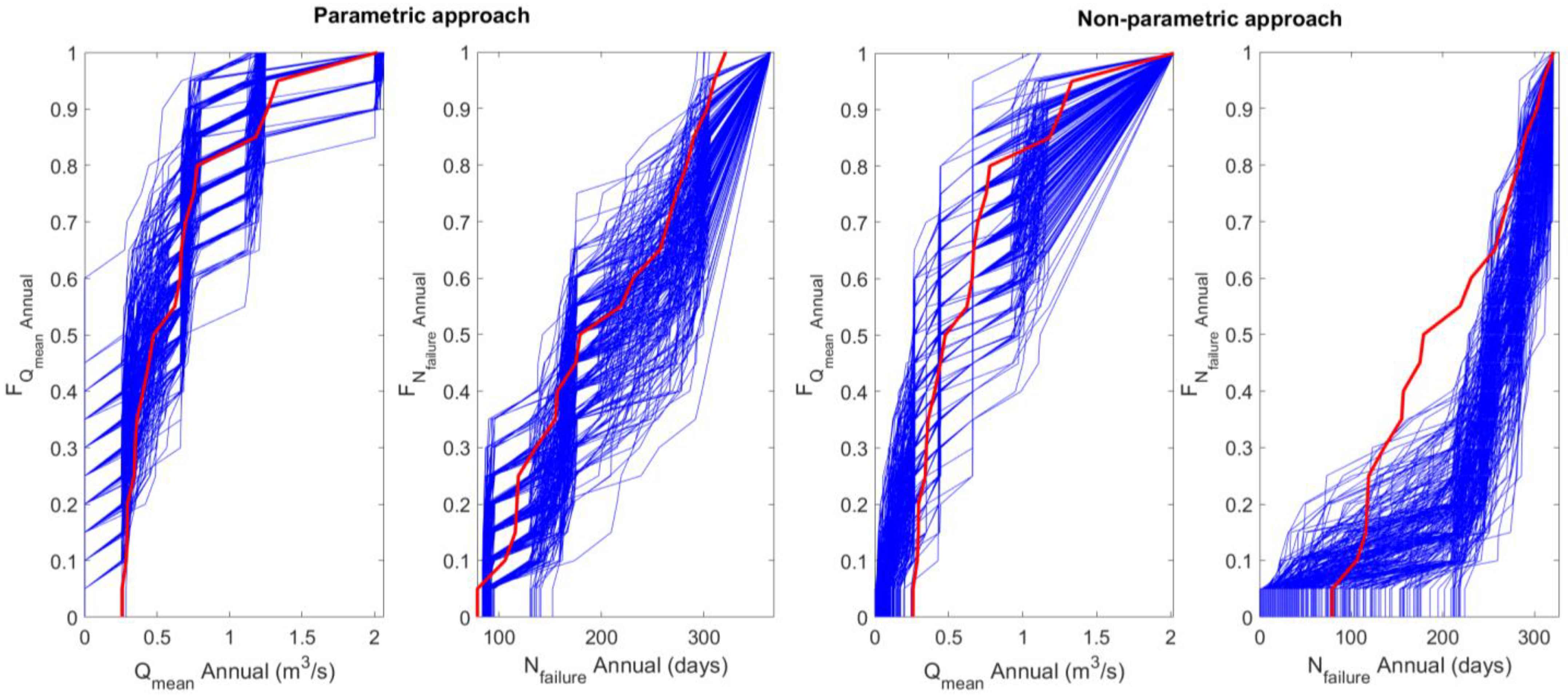
In Figure 5, the cdf of both the parametric and non-parametric methods is shown for the target variables Qmean and Nfailure. The empirical cdf of each variable obtained from observed data is represented in red. With both methods, the distribution of the mean river flow was reproduced using the 250 replications, with greater dispersion in the case of the non-parametric method, where, for instance, for 1 m3/s of the mean river flow, the probability was between 0.63 and 0.95 using the parametric method and between 0.4 and 0.95 using the non-parametric method (Figure 5).
In the case of the target variable, the number of days of failure, the parametric method properly reproduced the shape of the empirical cdf. In contrast, the non-parametric method clearly overestimated the value of this variable; that is, this method gave lower probabilities for a higher number of days of failure than what actually occurred, and the stochastic replications did not encompass the empirical cdf distribution of the variable.
A comparison of the basic statistics of both the observed and simulated series is presented in Table 6. The quantiles of the simulated series are of the same order of magnitude as the observed series, notably for the parametric method (e.g., 0.48 m3/s for the 50th percentile of the mean annual daily river flow). For the number of days of failure, the non-parametric method adequately reproduced the extremes of the distribution (e.g., 71 days for the fifth percentile and 310 days for the 90th percentile), although this method overestimated the value of the variable for the 50th percentile (267 days instead of 179 days in the observed series).
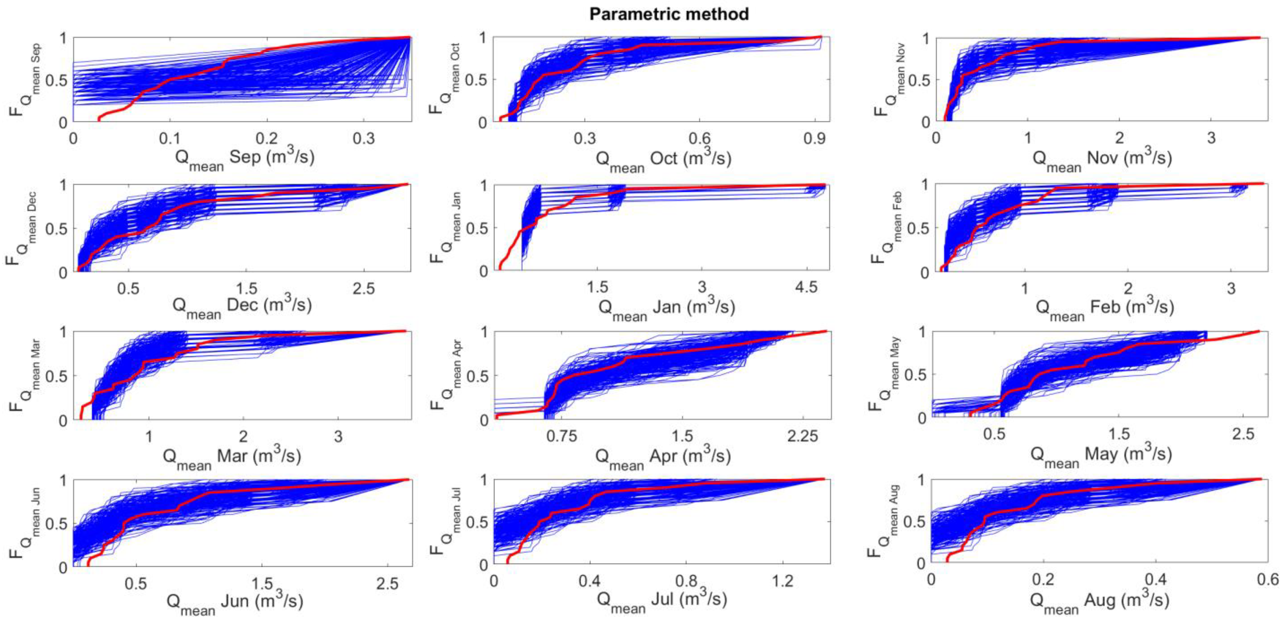
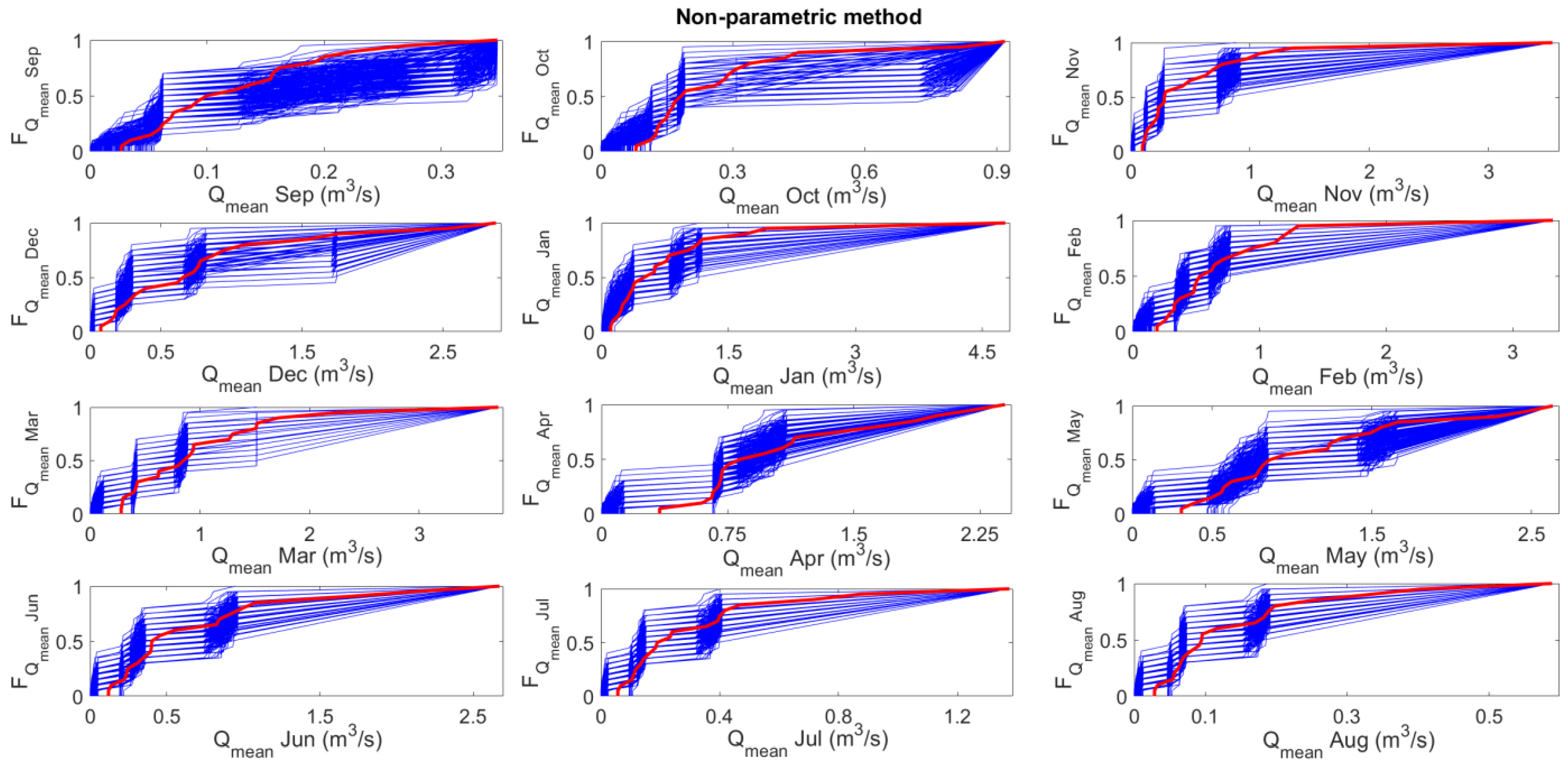
Regarding the monthly scale, in most months, both methods properly reproduced the shape of the empirical distribution functions of the mean monthly daily flow (Figure 6 and Figure 7), except in September, when the non-parametric method (Figure 7) encompassed the shape of the empirical distribution function. However, a greater dispersion was observed in the monthly daily flow predictions made using the non-parametric method in all the remaining months (Figure 7), being greater in September, October, December, and May.
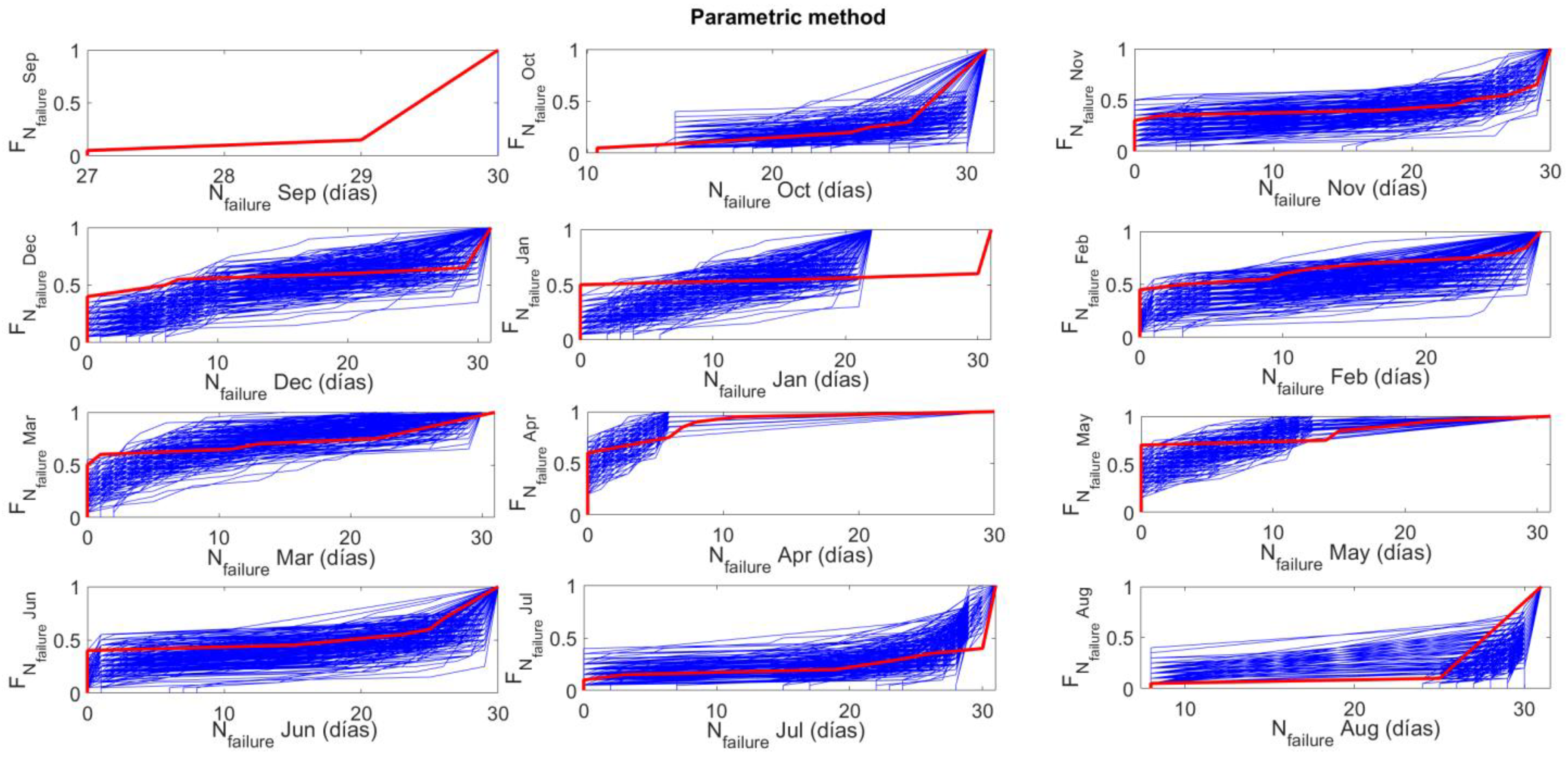
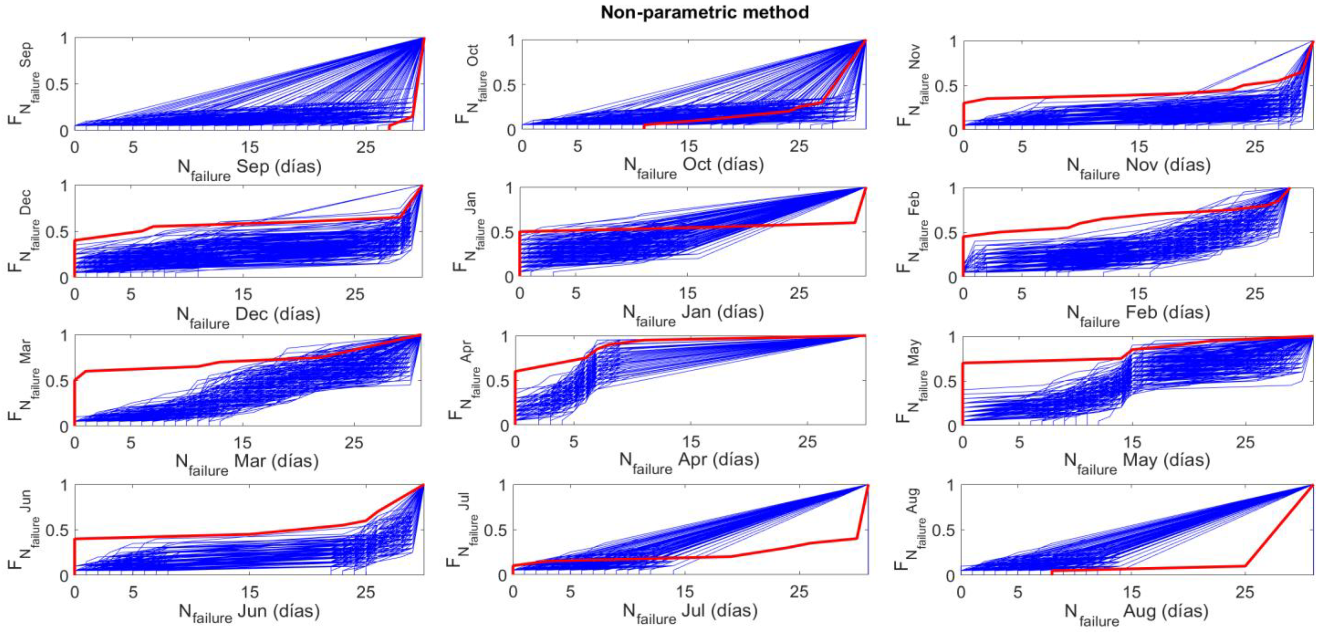
Similarly, for the variable number of days of failure, the parametric method (Figure 8) best reproduced the shape of the empirical distribution function than the non-parametric method (Figure 9), with the worst fits being those for September and January. In all cases (Figure 8 and Figure 9), the dispersion was greater for this variable, with a tendency to assign lower probabilities to higher failure values, i.e., to more days of failure in the month, in the same way as at the annual scale, especially in the months from November to June.
3.2.2. Operationality Assessment
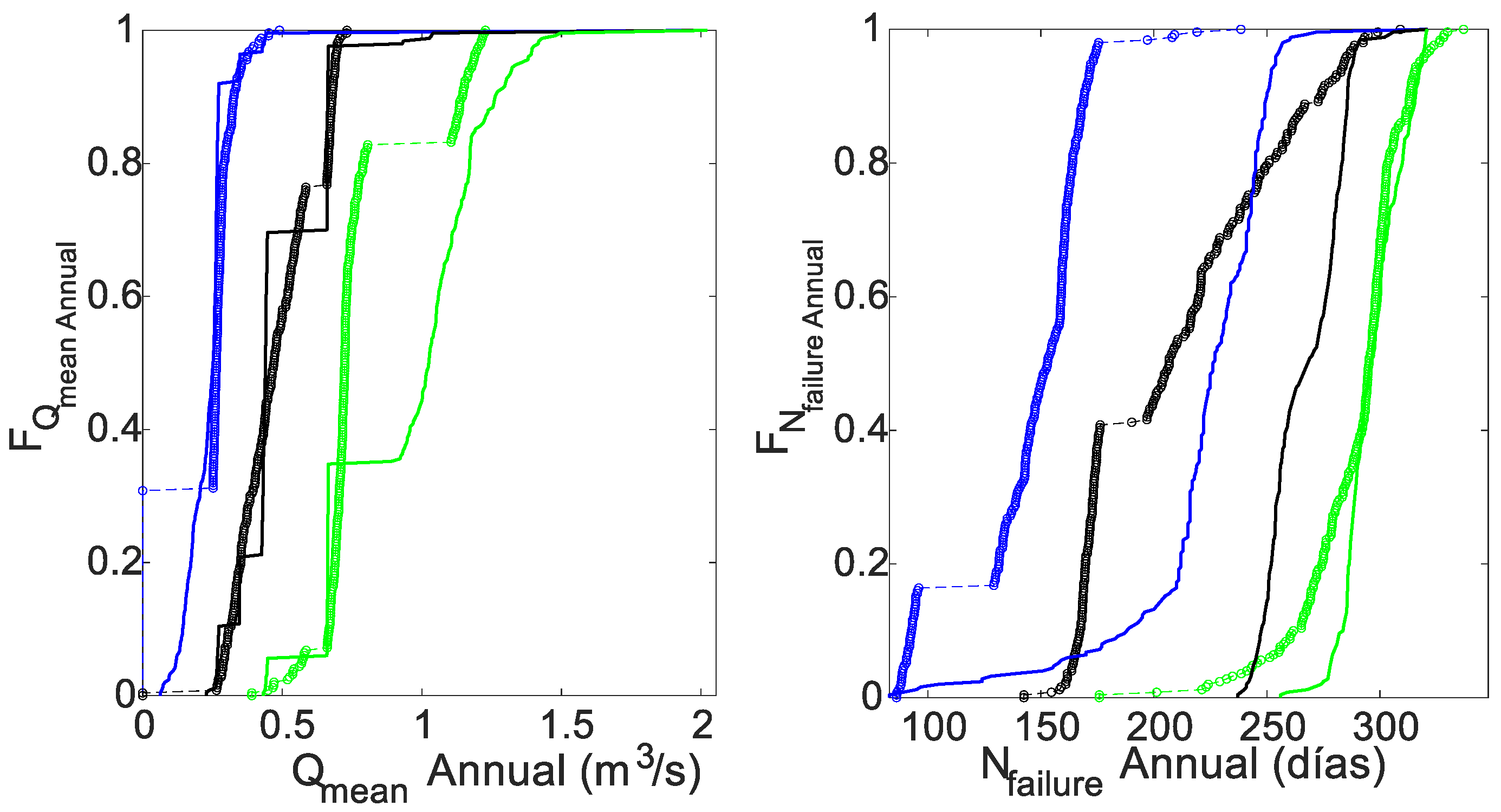
In the decision-making support process, the distribution functions of quartiles 1, 2, and 3 were obtained for both the mean daily river flow and the number of days of failure at the annual and monthly scales. At the annual scale (Figure 10), with both methods, the probability of having an annual mean river flow of 0.45 m3/s is 25%, whereas the probability of having an annual mean river flow of 0.73 m3/s is 50%, with the greatest difference between the methods found in the case of quartile 3 (75% probability). Regarding the variable number of days of failure, as shown in Figure 10, with the non-parametric method, a tendency to assign a higher number of days of failure to the three quartiles was observed. Unlike with the mean daily river flow, great differences between the methods were found in the cases of quartiles 1 and 2, whereas the results obtained with both approaches are practically the same for a 75% probability.
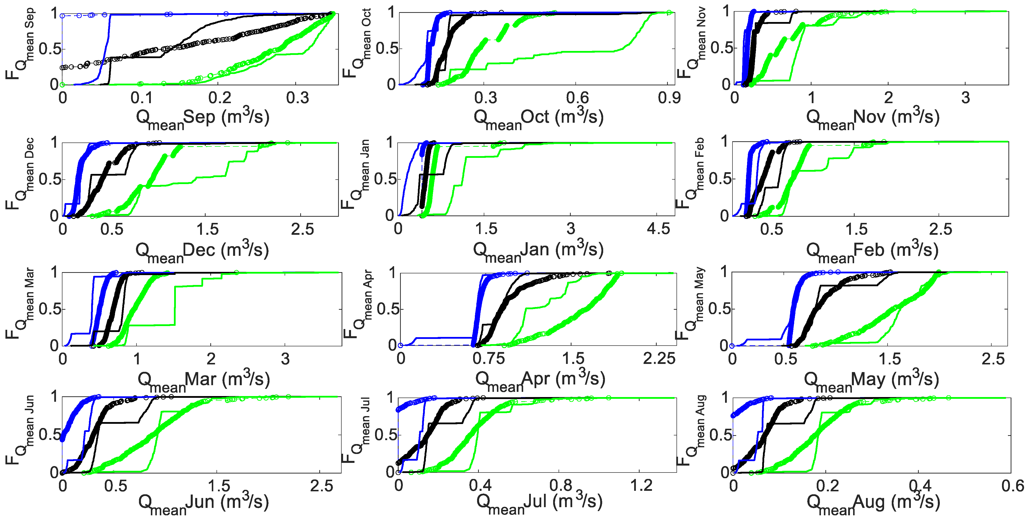
At the monthly scale and with respect to the mean monthly daily river flow (Figure 11), the results reveal that both methods show similar tendencies in terms of the distribution of quartiles 1 and 2 in all months, with some greater differences in the 75th percentile, especially in the months of October and December and from January to April.
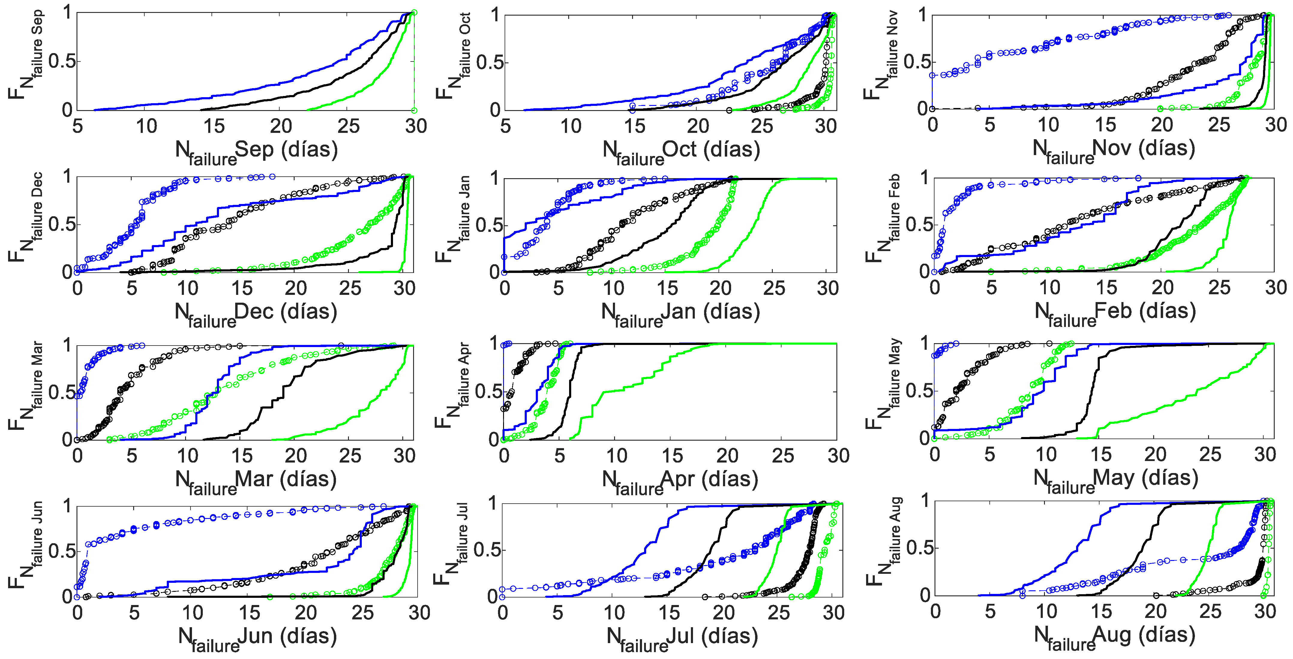
Regarding the number of days of failure (Figure 12), the results show that higher operationality occurs in the snowmelt season between April and May, with a 25% probability of having fewer than 1 and 2 days of failure, respectively (Figure 12), according to the parametric method, which increases to 5–12 days with a 75% probability. In the winter months (December to March), there is a 25% probability of having fewer than 12 days of failure (Figure 12). These results again reveal the influence of snowmelt, along with its effect on the increase in flow rates in the spring months and, thus, fewer days of failure.
3.3. Scenario Analysis
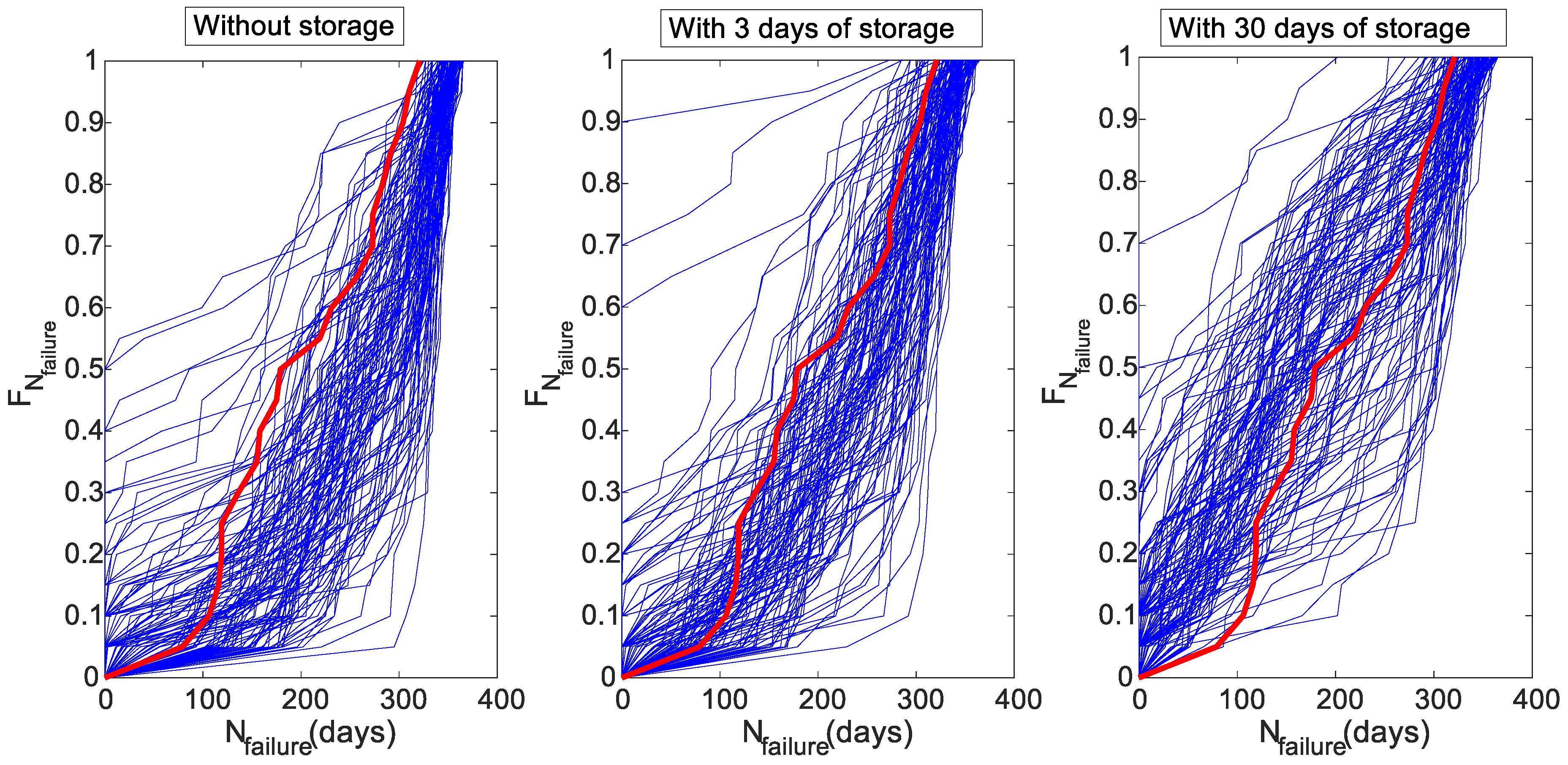
Figure 13 shows the distribution functions of the number of days of failure at the annual scale for the different storage scenarios. Obviously, there is a shift in the cdf toward the left (lower number of days of failure) of the stochastic cdf with a higher volume stored, and thus, higher frequencies for a lower number of days of failure when the storage is included can be observed, being more pronounced in the case of 30 days of storage. Thus, with a 90% probability, the number of days of failure in the scenario without storage ranges between 239 and 354 days. However, in the scenario with 3 days of storage, 0 days of failure were reached in one of the simulations, although it can be considered that with a 90% probability, the range decreases to between 226 and 350 days of annual failure. Finally, for the scenario with 30 days of storage, the range of the number of days of failure changes from 151 to 350 days, i.e., the lower limit of this interval significantly decreased.
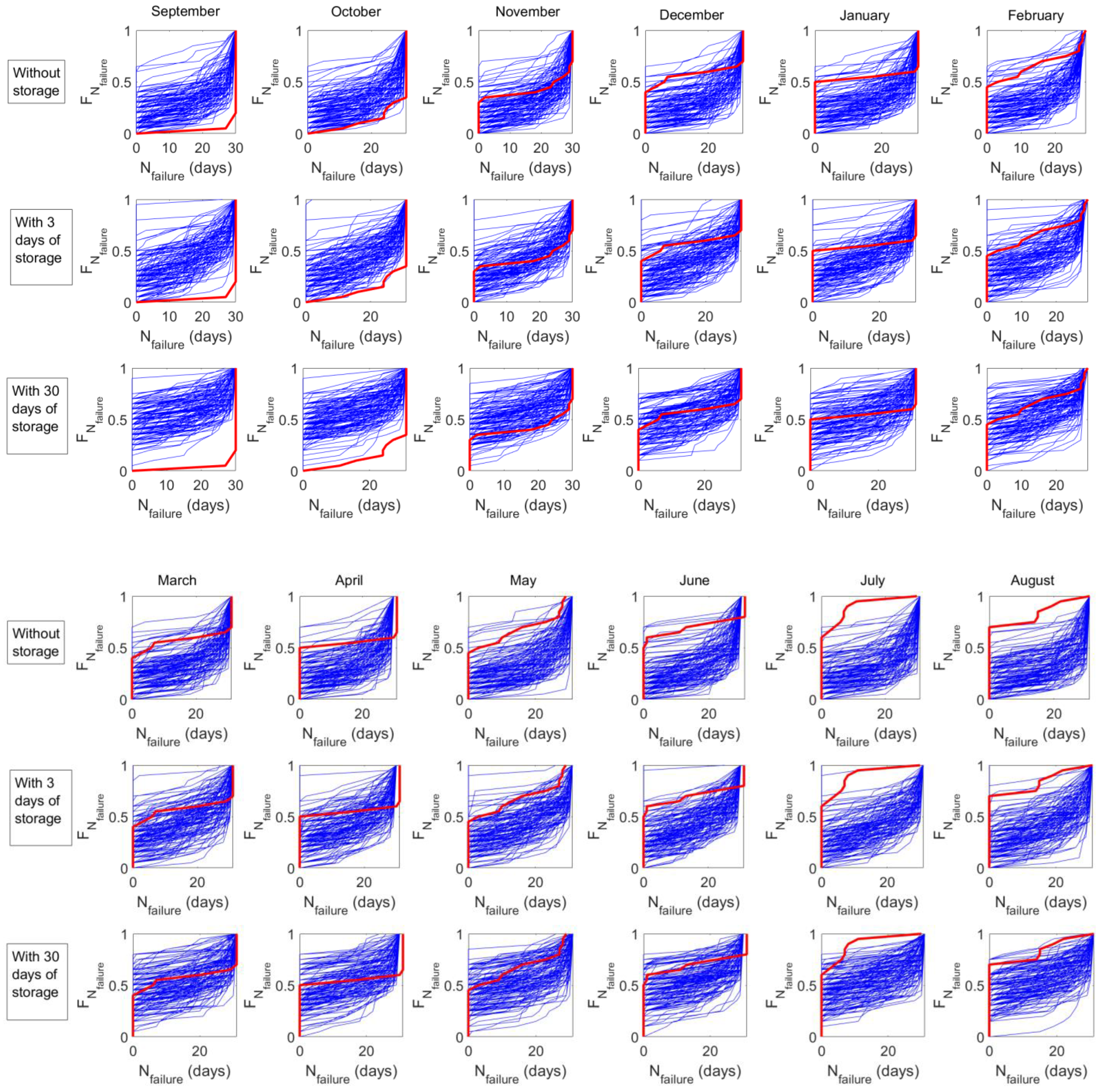
At the monthly time scale (Figure 14), the same trend was observed, with the effect of the water storage being greater in the months between June and November, when there are very few rainfall events and the snowmelt has almost finished. Thus, the effect of the decrease in the flow regime is compensated by the storage in the loading chamber. As an example, for this scale, in July, the range of probabilities for 15 days of failure is between 0.036 and 0.76 if there is no storage, between 0.1 and 0.76 in the scenario of 3 days of storage, and increasing to between 0.25 and 0.87 for the scenario of higher storage. This variation in percentages is greater in the month of November, where the probability of 15 days of plant operation failure is between 0.04 and 0.74 when there is no storage, between 0.1 and 0.87 when there are 3 days of storage, and increasing to between 0.25 and 0.9 for the case of 30 days of storage.
4. Discussion
The operation of run-of-river plants in Mediterranean mountainous basins is highly sensitive to the natural inflows to the plants. The challenge of snow-dominated Mediterranean mountainous RoR plants is the strong seasonality and interannual variability of river flows, as well as the input data availability to implement other existing data-demanding forecasting tools. Thus, this study proposes a new simple seasonal forecasting system that integrates the dynamic effect of the precipitation regime as a valuable tool for decision-making and action plans for strongly heterogeneous Mediterranean watersheds, where the straightforward application of other existing tools is not feasible nowadays due to the limitations of the input data requirements.
A seasonal forecasting system with limited uncertainty and sufficient reliability for decision-making means an improvement in their seasonal and annual planning, as well as a reduction in opportunity costs due to the lack of such a forecast.
First, significant forcing agents that allow for anticipating the regime of river inflows to RoR hydroelectric power plants need to be identified at each temporal scale. The best correlations were found between the mean daily flow and the average rainfall at the annual scale. At the monthly scale, different lag times in the influence of rainfall accumulated in the antecedent months had to be considered to capture its non-instantaneous impact on the river flows. These variable monthly lag times corresponded to the three main types of monthly river flows that mainly depend on rainfall (September–December), snowfall (January–February) and snowmelt (March–August), respectively. As for the monthly number of days of failure, an effect of the lag time influence of rivers was not observed, so the mean river flow of the same month can be considered the target forecast.
The results of this study are conditioned by the quality of the input data and the goodness of the calibration obtained with the model used to generate the distributed maps of the hydrometeorological variables analyzed, as well as the flow data series. Furthermore, the parametric approach is based on the best fits obtained among the variables, which introduces additional uncertainty associated with them.
The best statistical forecasts of the target variables were obtained with the parametric method in this case study. However, the non-parametric approach constitutes a very interesting option as a first evaluation as well as when parametric adjustments among variables with a high correlation are not available for the study site.
Despite the limitations stated above, our results allow for implementing a simple methodology to evaluate the operationality of the plant with natural inflows. The study of the operation of hydroelectric plants at annual and monthly scales allows for the inclusion of forecast precipitation and flow data generated by the European Centre for Medium-Range Weather Forecasts (ECMWF), available through the Copernicus Climate Change Service (C3S) [31,32,33]. With these data, the simple forecasting system presented here allows for performing a monthly forecast of the operationality and the number of days of failure of run-of-river hydroelectric plants six months ahead. Thus, the potential impact on water resource management and renewable energy generation is straightforward. The application of this approach in any other RoR plant only requires the proper identification of the forcing variable or target forecasts at each temporal scale of interest and parametric adjustments if the parametric approach is the chosen option. Nevertheless, the uncertainty of the forecasts will depend on the length and quality of the available hydrometeorological data series.
Previous studies have assessed the impact of changes in hydrometeorological conditions on various aspects of electrical power and energy systems (e.g., electricity generation, electricity consumption, etc.) [34]. Making energy infrastructures resilient to climate change requires dedicated policies and sophisticated decision-making measures to build adaptive capacity [35]. In this context, the proposed methodology constitutes a useful tool to assess uncertainty in the operationality of RoR plants and can be supported by forecast information through climate services [36,37]. The development of decision support tools for water management in hydroelectric plants is determined to minimize the impact of the variability in the flow regime in the medium and long term in the case of RoR hydroelectric plants. In these plants, the availability of water storage is limited or non-existent, so this type of tool makes it possible to limit the uncertainty associated with the production of the hydroelectric plant on a monthly and seasonal scale, at least six months in advance. Thus, this methodology can assist hydropower systems as the managers can plan the production of the plant at the beginning of the calendar year until the end of the snowmelt, as well as maintenance shutdowns of the plants during months of lower productivity.
5. Conclusions
A Bayesian dynamics stochastic model was developed in this study based on the simulation of rainfall with Monte Carlo at the annual and monthly scales, combining two methods—parametric and non-parametric. The best statistical forecasts of the target variables, the mean daily river flow and the number of days of failure, were obtained with the parametric method based on the best adjustments at each temporal scale considered. The results show a greater dispersion in the variable number of days of failure, with a tendency to assign lower probabilities to higher failure values. The operationality assessment performed showed the influence of snowmelt and its effect on the increase in flow rates in the spring months, with a 25% probability of having 1 and 2 days of failure in April and May, respectively, while in the winter months, this probability of 25% corresponds to having fewer than 12 days of failure and close to 30 days of failure in the remaining months.
A scenario analysis was carried out with the inclusion of water storage in the load chamber of hydroelectric plants and assessing its effect on the variable number of days of failure as a measure of the plant’s operationality. The results show the expected trends: the higher the load chamber considered, the higher the operationality level, and 239 to 151 annual days of failure without storage and with 30 days of storage, respectively, with a 90% probability. Regarding the monthly scale, the effect of water storage is greater in the months between June and November, with an operationality level of 0.04–0.74 for 15 days of failure without storage in November and of 0.25–0.9 with 30 days of storage.
Author Contributions
Conceptualization, R.G.-B. and C.A.; methodology, C.A. and R.G.-B.; validation, R.G.-B. and C.A.; formal analysis, C.A. and M.J.P.; investigation, R.G.-B., E.C. and C.A.; resources, C.A. and M.J.P.; writing—original draft preparation, R.G.-B.; writing—review and editing, R.G.-B. and C.A.; supervision, C.A. and M.J.P.; project administration, C.A. and M.J.P.; funding acquisition, C.A., E.C. and M.J.P. All authors have read and agreed to the published version of the manuscript.
Funding
This work has been funded by project 1381239-R “Herramienta de pronóstico estocástico de caudal para gestión de centrales hidroeléctricas en cuencas mediterráneas a distintas escalas temporales” with the economic collaboration of the European Funding for Rural Development (FEDER) and the Office for Economy, Knowledge, Enterprises and University of the Andalusian Regional Government; and by proyect PID2021-12323SNB-I00 “Incorporating hydrological uncertainty and risk analysis to the operation of hydropower facilities in Mediterranean mountain watersheds (HYPOMED)”, funding by Spanish Ministry of Science and Innovation MCIN/AEI/10.13039/501100011033/FEDER, UE.
Data Availability Statement
The data are not publicly available due to the authors do not have permission to share data.
Acknowledgments
Authors are thankful for the support and technical knowledge provided by the Poqueira hydropower system managers and personnel and the hydrological data provided by all the weather and hydrological networks in the study site.
Conflicts of Interest
The authors declare no conflicts of interests. The funders had no role in the design of the study; in the collection, analyses, or interpretation of data; in the writing of the manuscript; or in the decision to publish the results.
Appendix A
Table A1 and Table A2 show, respectively the fits and correlation coefficients (R2) at annual and monthly scale, between the mean river flow (Qmean) and rainfall (R), and between the number of days of failure (Nfailure) and the mean river flow (Qmean).

Table A1.
Fits and correlation coefficients (R2) between mean river flow (Qmean) at annual and monthly scale and rainfall (R).
Table A1.
Fits and correlation coefficients (R2) between mean river flow (Qmean) at annual and monthly scale and rainfall (R).
| River Flow Forecast | Forecasting from Rainfall of | Relationship | R2 |
|---|---|---|---|
| Annual | Annual | 0.99 | |
| January | December | 0.92 | |
| February | December and January | 0.91 | |
| March | February and March | 0.83 | |
| April | February to April | 0.80 | |
| May | February to May | 0.71 | |
| June | February to June | 0.80 | |
| July | February to June | 0.80 | |
| August | February to June | 0.82 | |
| September | September | 0.33 | |
| October | September and October | 0.83 | |
| November | October and November | 0.94 | |
| December | November and December | 0.78 |
The variable number of days of failure acts as a discrete variable in its extreme values, given by the limits of turbine operation in the hydroelectric plant. Therefore, to prepare the parametric adjustments for this variable, the same limits have been respected as for the turbine. That is, when the flow variable on the corresponding scale gives a value lower than the minimum turbine speed, the maximum value of the corresponding scale is assigned to the variable number of days of failure. Similarly, the flow value in the river flow above which there is no operational failure in the hydroelectric plant at the scale considered has been identified. Between these values, a parametric adjustment has been made for each month.
Table A2.
Fits and correlation coefficients (R2) between number of days of failure (Nfailure) and mean river flow (Qmean) at annual or monthly scale. The forecasting river flow month is the same than the forecast target month for Nfailure.
Table A2.
Fits and correlation coefficients (R2) between number of days of failure (Nfailure) and mean river flow (Qmean) at annual or monthly scale. The forecasting river flow month is the same than the forecast target month for Nfailure.
| Nfailure Forecast | Forecasting from River Flow of | Relationship | R2 |
|---|---|---|---|
| Annual mean | Annual mean | 0.89 | |
| January | January | 0.95 | |
| February | February | 0.93 | |
| March | March | 0.91 | |
| April | April | 0.88 | |
| May | May | 0.86 | |
| June | June | 0.93 | |
| July | July | 0.98 | |
| August | August | 0.99 | |
| September | September | -- | -- |
| October | October | 0.97 | |
| November | November | 0.89 | |
| December | December | 0.84 |
References
- Yildiz, V.; Vrugt, J.A. A toolbox for the optimal design of run-of-river hydropower plants. Environ. Model. Softw. 2019, 111, 34–152. [Google Scholar] [CrossRef]
- Contreras, E.; Herrero, J.; Crochemore, L.; Pechlivanidis, I.; Photiadou, C.; Aguilar, C.; Polo, M.J. Advances in the Definition of Needs and Specifications for a Climate Service Tool Aimed at Small Hydropower Plants’ Operation and Management. Energies 2020, 13, 1827. [Google Scholar] [CrossRef]
- Manzano-Agugliaro, F.; Tahera, M.; Zapata-Sierra, A.; Del Juaidi, A.; Montoya, F.G. An overview of research and energy evolution for small hydropower in Europe. Renew. Sustain. Energy Rev. 2017, 75, 476–489. [Google Scholar] [CrossRef]
- EnAppSys. European Electricity Fuel Mix Summary. Quarterly EU Market Summary, January to March. 2020. Available online: https://b74bc22f-390f-4347-ba45-b13ad13072ee.filesusr.com/ugd/9b26cb_80a91d80583e4c0e8c71ba3211517e3c.pdf (accessed on 27 March 2024).
- Saeed, A.; Shahzad, E.; Khan, A.U.; Waseem, A.; Iqbal, M.; Ullah, K.; Aslam, S. Three-Pond Model with Fuzzy Inference System-Based Water Level Regulation Scheme for Run-of-River Hydropower Plant. Energies 2023, 16, 2678. [Google Scholar] [CrossRef]
- Tsuanyo, D.; Amougou, B.; Aziz, A.; Nka Nnomo, B.; Fioriti, D.; Kenfack, J. Design models for small run-of-river hydropower plants: A review. Sustain. Energy Res. 2023, 10, 3. [Google Scholar] [CrossRef]
- Sojka, M. Directions and Extent of Flows Changes in Warta River Basin (Poland) in the Context of the Efficiency of Run-of-River Hydropower Plants and the Perspectives for Their Future Development. Energies 2022, 15, 439. [Google Scholar] [CrossRef]
- Pimentel, R.; Photiadou, C.; Little, L.; Huber, A.; Lemoine, A.; Leidinger, D.; Lira-Loarca, A.; Lückenkötter, J.; Pasten-Zapata, E. Improving the usability of climate services for the water sector: The AQUACLEW experience. Clim. Serv. 2022, 28, 100329. [Google Scholar] [CrossRef]
- Tobias, W.; Manfred, S.; Klaus, J.; Massimiliano, Z.; Bettina, S. The future of Alpline Run-of-River hydropower production: Climate change, environmental flow requirements, and technical production potential. Sci Total Environ. 2023, 890, 163934. [Google Scholar] [CrossRef] [PubMed]
- Viviroli, D.; Dürr, H.; Messerli, B.; Meybeck, M.; Weingartner, R. Mountains of the world, water tower for humanity: Typology, mapping, and global significance. Water Resour. Res. 2007, 43, W07447. [Google Scholar] [CrossRef]
- Pimentel, R.; Herrero, J.; Polo, M.J. Subgrid Parameterization of Snow Distribution at a Mediterranean Site Using Terrestrial Photography. Hydrol. Earth Syst. Sci. 2017, 21, 805–820. Available online: https://hess.copernicus.org/articles/21/805/2017/ (accessed on 27 March 2024). [CrossRef]
- Sakki, G.K.; Tsoukalas, I.; Kossieris, P.; Makropoulos, C.; Efstratiadis, A. Stochastic simulation-optimization framework for the design and assessment of renewable energy systems under uncertainty. Renew. Sust. Energy Rev. 2022, 168, 112886. [Google Scholar] [CrossRef]
- Aguilar, C.; Polo, M.J. Assessing minimum environmental flows in nonpermanent rivers: The choice of thresholds. Environ. Model. Soft. 2016, 79, 102–134. [Google Scholar] [CrossRef]
- Kottegoda, N.T.; Rosso, R. Applied Statistics for Civil and Environmental Engineers, 2nd ed.; Blackwell Publishing Ltd.: Oxford, UK, 2008; ISBN 978-1-4051-7917-1. [Google Scholar]
- Kottegoda, N.T.; Natale, L.; Raiteri, E. Monte Carlo Simulation of rainfall hyetographs for analysis and design. J. Hydrol. 2014, 519, 1–11. [Google Scholar] [CrossRef]
- Polo, M.J.; Herrero, J.; Pimentel, R.; Pérez-Palazón, M.J. The Guadalfeo Monitoring Network (Sierra Nevada, Spain): 14 Years of Measurements to Understand the Complexity of Snow Dynamics in Semiarid Regions. Earth Syst. Sci. Data. 2019, 11, 393–407. Available online: https://essd.copernicus.org/articles/11/393/2019/ (accessed on 27 March 2024). [CrossRef]
- Authomatic Hydrological Information System (SAIH). Andalusian Government. Available online: http://www.redhidrosurmedioambiente.es/saih/ (accessed on 27 March 2024).
- AEMET: AEMET Open Data, AEMET [Data Set]. Available online: https://www.aemet.es/es/datos_abiertos, (accessed on 27 March 2024).
- Gan, K.C.; McMahon, T.A.; Finlayson, B.L. Analysis of periodicity in streamflow and rainfall data by Colwell’s indices. J. Hydrol. 1991, 123, 105–118. [Google Scholar] [CrossRef]
- Brunner, M.I.; Björnsen Gurung, A.; Zappa, M.; Zekollari, H.; Farinotti, D.; Stähli, M. Present and future water scarcity in Switzerland: Potential for alleviation through reservoirs and lakes. Sci. Total Environ. 2019, 666, 1033–1047. [Google Scholar] [CrossRef] [PubMed]
- Polo, M.J.; Herrero, J.; Aguilar, C.; Millares, A.; Moñino, A.; Nieto, S.; Losada, M.A. WiMMed, a Distributed Physically-Based Watershed Model (I): Description and Validation. In Theorical, Experimental and Computational Solutions, Proceedings of the International Workshop on Environmental Hydraulics 09, Valencia, Spain, 28–29 October 2009; Taylor & Francis: Valencia, Spain, 2009; pp. 225–228. [Google Scholar]
- Egüen, M.; Aguilar, C.; Solari, S.; Losada, M.A. Non-stationary rainfall and natural flows modeling at the watershed scale. J. Hydrol. 2016, 538, 767–782. [Google Scholar] [CrossRef]
- Pastén-Zapata, E.; Pimentel, R.; Royer-Gaspard, P.; Sonnenborg, T.O.; Aparicio-Ibañez, J.; Lemoine, A.; Pérez-Palazón, M.J.; Schneider, R.; Photiadou, C.; Thirel, G.; et al. The effect of weighting hydrological projections based on the robustness of hydrological models under a changing climate. J. Hydrol. Reg. Stud. 2022, 41, 101113. [Google Scholar] [CrossRef]
- Michaud, J.; Sorooshian, S. Effects of rainfall-sampling errors on simulations of desert flash floods. Water Resour. Res. 1994, 30, 2765–2775. [Google Scholar] [CrossRef]
- Zhao, F.; Zhang, L.; Chiew, F.H.S.; Vaze, J.; Cheng, L. The effect of spatial rainfall variability on water balance modelling for south-eastern Australian catchments. J. Hydrol. 2013, 493, 16–29. [Google Scholar] [CrossRef]
- Godinho, F.; Costa, S.; Pinheiro, P.; Reis, F.; Pinheiro, A. Integrated procedure for environmental flow assessment in rivers. Environ. Process. 2014, 1, 137–147. [Google Scholar] [CrossRef]
- Fill, H.D.; Steiner, A.A. Estimating instantaneous peak flow from mean daily flow data. J. Hydrol. Eng. 2003, 8, 365–369. [Google Scholar] [CrossRef]
- Taguas, E.V.; Ayuso, J.L.; Peña, A.; Yuan, Y.; Sanchez, M.C.; Giraldez, J.V.; Perez, R. Testing the relationship between instantaneous peak flow and mean daily flow in a Mediterranean Area Southeast Spain. Catena. 2008, 75, 129–137. [Google Scholar] [CrossRef]
- Ho, L.T.T.; Dubus, L.; De Felice, M.; Troccoli, A. Reconstruction of Multidecadal Country-Aggregated Hydro Power Generation in Europe Based on a Random Forest Model. Energies 2020, 13, 1786. [Google Scholar] [CrossRef]
- Polo, M.J.; Aguilar, C.; Millares, A.; Herrero, J.; Gómez-Beas, R.; Contreras, E.; Losada, M.A. Assessing risks for integrated water resource management: Coping with uncertainty and the human factor. Proc. IAHS 2014, 364, 285e291. Available online: https://piahs.copernicus.org/articles/364/285/2014/ (accessed on 14 February 2024). [CrossRef]
- Crochemore, L.; Ramos, M.-H.; Pechlivanidis, I.G. Can Continental Models Convey Useful Seasonal Hydrologic Information at the Catchment Scale? Water Resour. Res. 2020, 56, e2019WR025700. [Google Scholar] [CrossRef]
- Pechlivanidis, I.; Crochemore, L.; Bosshard, T. Seasonal streamflow forecasting—Which are the drivers controlling the forecast quality? In Proceedings of the EGU General Assembly 2020, Vienna, Austria, 4–8 May 2020.
- Climate Change Copernicus. Available online: https://www.copernicus.eu/en/services/climate-change (accessed on 27 March 2024).
- Mohammadi, Y.; Palstev, A.; Polajžer, B.; Miraftabzadeh, S.M.; Khodadad, D. Investigating Winter Temperatures in Sweden and Norway: Potential Relationships with Climatic Indices and Effects on Electrical Power and Energy Systems. Energies 2023, 16, 5575. [Google Scholar] [CrossRef]
- Adaptation Challenges and Opportunities for the European Energy System. Building a Climate-Resilient Low-Carbon Energy System. Available online: https://www.eea.europa.eu/publications/adaptation-in-energy-system (accessed on 27 March 2024).
- Buizer, J.; Jacobs, K.; Cash, D. Making short-term climate forecasts useful: Linking science and action. Proc. Natl. Acad. Sci. USA 2016, 113, 4597–4602. [Google Scholar] [CrossRef]
- Dutton, J.A.; James, R.P.; Ross, J.D. Probabilistic Forecasts for Energy: Weeks to a Century or More. In Weather & Climate Services for the Energy Industry; Troccoli, A., Ed.; Springer: Cham, Switzerland, 2018; pp. 161–177. ISBN 978-3-319-68418-5. [Google Scholar]
Figure 1.
Location of the Poqueira River basin in southern Spain and the three RoR hydroelectric plants system in the study area.
Figure 1.
Location of the Poqueira River basin in southern Spain and the three RoR hydroelectric plants system in the study area.

Figure 2.
Results of hydrological simulation and measured river flow at study site.

Figure 3.
Calculation sequence of Bayesian dynamics forecast of water inputs: (a) parametric method (PM) and (b) non-parametric method (NPM). Blue lines are cdf of the 250 sets of 20-year series of equally probable rainfall (i), mean daily flow (ii), or number of days of failure (iii) obtained with Monte Carlo. In red, the empirical cdf obtained from the observed data.

Figure 5.
Cumulative distribution functions (cdf) of the mean annual daily river flow and the number of days of failure in the parametric and non-parametric methods. In red, the empirical cdf obtained from the observed data.
Figure 5.
Cumulative distribution functions (cdf) of the mean annual daily river flow and the number of days of failure in the parametric and non-parametric methods. In red, the empirical cdf obtained from the observed data.

Figure 6.
Cumulative distribution functions of monthly river flow using parametric method. In red, the empirical cdf obtained from the observed data.
Figure 6.
Cumulative distribution functions of monthly river flow using parametric method. In red, the empirical cdf obtained from the observed data.

Figure 7.
Cumulative distribution functions of monthly river flow using non-parametric method. In red, the empirical cdf obtained from the observed data.
Figure 7.
Cumulative distribution functions of monthly river flow using non-parametric method. In red, the empirical cdf obtained from the observed data.

Figure 8.
Cumulative distribution functions of monthly number of days of failure using parametric method. In red, the empirical cdf obtained from the observed data.
Figure 8.
Cumulative distribution functions of monthly number of days of failure using parametric method. In red, the empirical cdf obtained from the observed data.

Figure 9.
Cumulative distribution functions of monthly number of days of failure using non-parametric method. In red, the empirical cdf obtained from the observed data.
Figure 9.
Cumulative distribution functions of monthly number of days of failure using non-parametric method. In red, the empirical cdf obtained from the observed data.

Figure 10.
Cumulative distribution function of quartiles 1 (blue), 2 (black), and 3 (green) for annual river flow and number of days of failure using parametric method (circles) and non-parametric method (solid line).
Figure 10.
Cumulative distribution function of quartiles 1 (blue), 2 (black), and 3 (green) for annual river flow and number of days of failure using parametric method (circles) and non-parametric method (solid line).

Figure 11.
Cumulative distribution function of quartiles 1 (blue), 2 (black), and 3 (green) for monthly river flow using parametric method (circles) and non-parametric method (line).
Figure 11.
Cumulative distribution function of quartiles 1 (blue), 2 (black), and 3 (green) for monthly river flow using parametric method (circles) and non-parametric method (line).

Figure 12.
Cumulative distribution function of quartiles 1 (blue), 2 (black), and 3 (green) for monthly number of days of failure using parametric method (circles) and non-parametric method (line).
Figure 12.
Cumulative distribution function of quartiles 1 (blue), 2 (black), and 3 (green) for monthly number of days of failure using parametric method (circles) and non-parametric method (line).

Figure 13.
Cumulative distribution functions of number of days of failure in different storage scenarios: without storage, with 3 days of storage, and with 30 days of storage at annual scale. In red, the empirical cdf obtained from the observed data.
Figure 13.
Cumulative distribution functions of number of days of failure in different storage scenarios: without storage, with 3 days of storage, and with 30 days of storage at annual scale. In red, the empirical cdf obtained from the observed data.

Figure 14.
Cumulative distribution functions of number of days of failure in different storage scenarios: without storage, with 3 days of storage, and with 30 days of storage at monthly scale. In red, the empirical cdf obtained from the observed data.
Figure 14.
Cumulative distribution functions of number of days of failure in different storage scenarios: without storage, with 3 days of storage, and with 30 days of storage at monthly scale. In red, the empirical cdf obtained from the observed data.

Table 1.
HP1 characteristics.
| Characteristic | Value |
|---|---|
| Generation capacity | 14.4 MW |
| Net jump | 570 m |
| Nominal turbine flow | 2.5 m3/s |
Table 2.
Mean, maximum, minimum, and standard deviation values of the mean daily river flow (Q), accumulated rainfall (R), snow water equivalent (SWE), and snowmelt (SWM) in the contributing basin to the HP1 power plant at the annual and monthly scales.
Table 2.
Mean, maximum, minimum, and standard deviation values of the mean daily river flow (Q), accumulated rainfall (R), snow water equivalent (SWE), and snowmelt (SWM) in the contributing basin to the HP1 power plant at the annual and monthly scales.
| Annual | Sep | Oct | Nov | Dec | Jan | Feb | Mar | Apr | May | Jun | Jul | Aug | ||
|---|---|---|---|---|---|---|---|---|---|---|---|---|---|---|
| R (mm) | Mean | 874.7 | 45.5 | 103 | 121.5 | 129.4 | 80.1 | 105.3 | 115.8 | 96.3 | 55.1 | 12.5 | 2.1 | 8.2 |
| Max | 1804.5 | 104 | 266.5 | 280.3 | 684.5 | 271.3 | 384 | 397.6 | 192.4 | 184.5 | 45.6 | 9.6 | 35.9 | |
| Min | 485.6 | 0.55 | 18.8 | 18.9 | 0.98 | 4.9 | 0 | 22.6 | 4.1 | 5.8 | 0 | 0 | 0 | |
| S. D. | 318.3 | 33.1 | 73 | 82.3 | 167.6 | 68.2 | 83.4 | 90.2 | 51.1 | 53.6 | 12.4 | 3 | 10.4 | |
| Q (m3/s) | Mean | 0.7 | 0.13 | 0.28 | 0.61 | 0.85 | 0.9 | 0.78 | 1.06 | 1.1 | 1.15 | 0.75 | 0.34 | 0.16 |
| Max | 2.0 | 0.35 | 0.92 | 3.5 | 2.9 | 4.8 | 3.3 | 3.7 | 2.4 | 2.6 | 2.7 | 1.4 | 0.59 | |
| Min | 0.3 | 0.03 | 0.08 | 0.10 | 0.08 | 0.11 | 0.19 | 0.28 | 0.35 | 0.31 | 0.12 | 0.06 | 0.03 | |
| S. D. | 0.5 | 0.08 | 0.23 | 0.78 | 0.78 | 1.05 | 0.69 | 0.83 | 0.60 | 0.69 | 0.69 | 0.33 | 0.14 | |
| SWE (mm) | Mean | 10,392 | 0.39 | 22.2 | 408.1 | 1154.7 | 1640.2 | 1854.8 | 2434.3 | 1784.3 | 938.2 | 147.9 | 6.9 | 0.07 |
| Max | 42,029 | 7.7 | 94.4 | 2036 | 3889 | 6399 | 7886 | 10581 | 8506 | 5509 | 1352 | 121.9 | 1.4 | |
| Min | 1497.7 | 0 | 0 | 4.9 | 54.8 | 28.3 | 103.3 | 63.9 | 213.1 | 4.24 | 0 | 0 | 0 | |
| S. D. | 10,143 | 1.71 | 30.2 | 500 | 1076.7 | 1766.2 | 1955.1 | 2554.4 | 2021.3 | 1405.2 | 316.3 | 27.13 | 0.31 | |
| SWM (mm) | Mean | 263.8 | 0.25 | 4.3 | 17.6 | 30.4 | 25.6 | 29.4 | 49 | 54.5 | 39.1 | 12.7 | 0.9 | 0.02 |
| Max | 638.1 | 4.3 | 12.1 | 46.3 | 116.9 | 64.9 | 83 | 110.4 | 102.6 | 114.6 | 87.7 | 16.1 | 0.3 | |
| Min | 92.6 | 0 | 0.05 | 1.3 | 0.92 | 2.8 | 2.3 | 5.2 | 9.4 | 1.1 | 0 | 0 | 0 | |
| S. D. | 125.1 | 1 | 4.4 | 16.5 | 28.2 | 15 | 19.6 | 28.2 | 26 | 33.7 | 22.8 | 3.6 | 0.07 |
Table 3.
R2 of the linear correlations among the following variables: Qmean (mean annual daily river flow), Qmax (maximum annual daily river flow), R (annual rainfall), ES (annual evaposublimation), S (annual snowfall), SWM (annual snowmelt), SWE (annual snow water equivalent), and Nfailure (annual number of days of failure). Values over 0.6 are in bold.
| Nfailure | Qmean | Qmax | R | Rmax | S | R − ES | SWM | SWE | |
|---|---|---|---|---|---|---|---|---|---|
| Nfailure | 1 | 0.63 | 0.33 | 0.65 | 0.19 | 0.36 | 0.64 | 0.38 | 0.41 |
| Qmean | 0.63 | 1.00 | 0.82 | 0.98 | 0.41 | 0.67 | 0.97 | 0.75 | 0.72 |
| Qmax | 0.33 | 0.82 | 1.00 | 0.80 | 0.52 | 0.43 | 0.82 | 0.51 | 0.51 |
| R | 0.65 | 0.98 | 0.80 | 1.00 | 0.41 | 0.67 | 0.99 | 0.74 | 0.72 |
| Rmax | 0.19 | 0.41 | 0.52 | 0.41 | 1.00 | 0.15 | 0.43 | 0.19 | 0.34 |
| S | 0.36 | 0.67 | 0.43 | 0.67 | 0.15 | 1.00 | 0.58 | 0.98 | 0.81 |
| R − ES | 0.64 | 0.97 | 0.82 | 0.99 | 0.43 | 0.58 | 1.00 | 0.67 | 0.66 |
| SWM | 0.38 | 0.75 | 0.51 | 0.74 | 0.19 | 0.98 | 0.67 | 1.00 | 0.85 |
| SWE | 0.41 | 0.72 | 0.51 | 0.72 | 0.34 | 0.81 | 0.66 | 0.85 | 1.00 |
Table 4.
Best correlation coefficients of the monthly mean daily flow with the variables analyzed. Values over 0.6 are in bold.
Table 4.
Best correlation coefficients of the monthly mean daily flow with the variables analyzed. Values over 0.6 are in bold.
| September | October | November | December | January | February | March | April | May | June | July | August | |
|---|---|---|---|---|---|---|---|---|---|---|---|---|
| Nfailure | 0.05 | 0.9 | 0.88 | 0.89 | 0.86 | 0.91 | 0.91 | 0.87 | 0.91 | 0.94 | 0.93 | 0.77 |
| Qm_max | 0.74 | 0.9 | 0.94 | 0.98 | 0.99 | 0.97 | 0.99 | 0.94 | 0.95 | 0.99 | 0.99 | 1 |
| Rm | 0.35 | 0.84 | 0.36 | 0.54 | 0.65 | 0.72 | 0.73 | 0.02 | 0.46 | 0.25 | 0.75 | 0.06 |
| Rm_prev | 0.05 | 0.35 | 0.72 | 0.5 | 0.92 | 0.77 | 0.59 | 0.74 | 0.16 | 0.38 | 0.36 | 0.71 |
| Rm_max | 0.07 | 0.76 | 0.03 | 0.48 | 0.44 | 0.49 | 0.41 | 0.22 | 0.34 | 0.46 | 0.73 | 0.36 |
| Rm_max_prev | 0.01 | 0.7 | 0.55 | 0.26 | 0.87 | 0.51 | 0.38 | 0.43 | 0.34 | 0.35 | 0.57 | 0.69 |
| Rm − ESm | 0.35 | 0.84 | 0.37 | 0.54 | 0.55 | 0.72 | 0.68 | 0.03 | 0.45 | 0.24 | 0.75 | 0.56 |
| Sm | 0.24 | 0.47 | 0.07 | 0.51 | 0.35 | 0.76 | 0.46 | 0.02 | 0.38 | 0.39 | -- | -- |
| Sm_prev | -- | 0.29 | 0.83 | 0.05 | 0.89 | 0.49 | 0.62 | 0.7 | 0.39 | 0.39 | 0.5 | -- |
| SWMm | 0.27 | 0.28 | 0.4 | 0.49 | 0.7 | 0.67 | 0.51 | 0.62 | 0.75 | 0.91 | 0.65 | -- |
| SWEm | 0.02 | 0.49 | 0.16 | 0.45 | 0.9 | 0.9 | 0.89 | 0.79 | 0.71 | 0.9 | 0.61 | -- |
Table 5.
Best correlation coefficients between accumulated rainfall and mean monthly river flow.
| River Flow Forecast | Forecasting from Rainfall of | R2 |
|---|---|---|
| January | December | 0.92 |
| February | December and January | 0.91 |
| March | February and March | 0.83 |
| April | February to April | 0.80 |
| May | February to May | 0.71 |
| June | February to June | 0.80 |
| July | February to June | 0.80 |
| August | February to June | 0.82 |
| September | September | 0.33 |
| October | September and October | 0.83 |
| November | October and November | 0.94 |
| December | November and December | 0.78 |
Table 6.
The 5th, 50th, and 90th percentiles (F5, F50, F90) of the observed and simulated mean annual river flow (Qmean, Qpmean, and Qnpmean m3/s) and number of days of failure (Nfailure, Npfailure, and Nnpfailure days), using the parametric and non-parametric methods. The statistics of the simulated series represent the average over the 250 replicates generated for each variable.
| Percentile | Qmean | Qpmean | Qnpmean | Nfailure | Npfailure | Nnpfailure |
|---|---|---|---|---|---|---|
| F5 | 0.26 | 0.004 | 0.056 | 79 | 88 | 71 |
| F50 | 0.48 | 0.48 | 0.51 | 179 | 210 | 267 |
| F90 | 1.26 | 1.15 | 1.48 | 303 | 325 | 310 |
Disclaimer/Publisher’s Note: The statements, opinions and data contained in all publications are solely those of the individual author(s) and contributor(s) and not of MDPI and/or the editor(s). MDPI and/or the editor(s) disclaim responsibility for any injury to people or property resulting from any ideas, methods, instructions or products referred to in the content. |
© 2024 by the authors. Licensee MDPI, Basel, Switzerland. This article is an open access article distributed under the terms and conditions of the Creative Commons Attribution (CC BY) license (https://creativecommons.org/licenses/by/4.0/).
Share and Cite
MDPI and ACS Style
Gómez-Beas, R.; Contreras, E.; Polo, M.J.; Aguilar, C. Stochastic Flow Analysis for Optimization of the Operationality in Run-of-River Hydroelectric Plants in Mountain Areas. Energies 2024, 17, 1705. https://doi.org/10.3390/en17071705
AMA Style
Gómez-Beas R, Contreras E, Polo MJ, Aguilar C. Stochastic Flow Analysis for Optimization of the Operationality in Run-of-River Hydroelectric Plants in Mountain Areas. Energies. 2024; 17(7):1705. https://doi.org/10.3390/en17071705
Chicago/Turabian StyleGómez-Beas, Raquel, Eva Contreras, María José Polo, and Cristina Aguilar. 2024. "Stochastic Flow Analysis for Optimization of the Operationality in Run-of-River Hydroelectric Plants in Mountain Areas" Energies 17, no. 7: 1705. https://doi.org/10.3390/en17071705
Note that from the first issue of 2016, this journal uses article numbers instead of page numbers. See further details here.