
Modeling of Linearized Generator Inertia Constraints for Unit Commitment


Department of Electronic and Electrical Engineering, Hongik University, Seoul 04066, Republic of Korea
*
Author to whom correspondence should be addressed.
Energies 2024, 17(5), 1120; https://doi.org/10.3390/en17051120
Submission received: 18 January 2024
/
Revised: 14 February 2024
/
Accepted: 21 February 2024
/
Published: 26 February 2024
(This article belongs to the Section F1: Electrical Power System)
Abstract
:This study presents a novel approach to modeling linearized inertia constraints of generators, considering frequency stability, and applies it to the unit commitment (UC). Specifically, we modeled the average rate of change of frequency (RoCoF) constraint and the minimum frequency constraint using the analytical expression derived from the reduced frequency response (RFR) model. We also considered the load-damping constant as a variable. As the power system has different nonlinear characteristics according to its operating status, the system can be expressed as several different systems. Each subsystem, with its own properties at a given operating point, is modeled as a single-machine system, categorized by pumped storage hydropower (PSH) status. The minimum frequency of each subsystem is determined by its individual machine time constant. We incorporated an additional constraint to ensure the quasi steady-state performance of frequency. This constraint can be omitted when it is not necessary. The proposed concepts have been validated on the Korean Power System. The UC, with the proposed inertia constraints, can secure system inertia and primary frequency response (PFR) that satisfies frequency stability. Our proposed method is more efficient in securing inertia and PFRs and more economical in terms of generation cost compared to existing methods.
1. Introduction
The inertia of a power system is its ability to resist frequency changes [1]. As the inertia of the power system decreases, frequency changes in response to supply and demand imbalances increase in intensity, and thus, maintaining the frequency stability of the system is challenging [2]. Currently, the inertia of power systems is gradually decreasing with the rising share of power supplied from asynchronous sources, such as wind or solar power [3,4,5,6,7,8,9]. To maintain frequency stability in these power systems, sufficient system inertia and primary frequency response (PFR) must be ensured. In this regard, studies have explored methods to secure the system inertia directly through synchronous condensers or to support the system inertia through power electronics such as the battery energy storage system [6,10]; however, the system inertia is fundamentally secured through synchronous generators. Thus, to maintain frequency stability, methods are needed to secure the system inertia in the unit commitment (UC) [9,10,11].
In an optimization problem, the method of securing system inertia is reflected as constraints. Early inertia constraints were simple, ensuring that the system had at least the critical inertia [3,4]. Auxiliary constraints, such as minimum available synchronous capacity or the maximum level of system non-synchronous penetration, were also used [9]. The critical inertia was either determined externally to the UC or through rate of change of frequency (RoCoF) constraints for contingencies [12,13,14]. The same methodology that applies to frequency constraints can be applied to maintain frequency stability with inertia constraints. In certain studies, the inertia constraints consist of RoCoF constraints and minimum frequency constraints for contingencies [11]. Moreover, quasi steady-state frequency constraints, which are not related to system inertia, are included in the inertia constraints to ensure frequency stability [9,15].
The RoCoF constraints have been modeled in most studies using the instantaneous RoCoF at the time of the contingency [15,16,17,18,19,20,21,22]. The advantage of using the instantaneous RoCoF is that the constraints are linear. However, in terms of the behavior of RoCoF protection relays, the constraint using the instantaneous RoCoF results in conservative securing of the system inertia, and reflecting the RoCoF improvement effect of fast response resources is a difficult task. In [23], the RoCoF constraint was modeled using the average RoCoF; however, the PFRs of synchronous generators and characteristics of load changes with respect to frequency changes were ignored.
The minimum frequency constraints require a separate linearization process owing to the nonlinearity of the analytical expression of the frequency. Certain studies have derived the analytical expression of the frequency by assuming that the PFRs of the synchronous generators operating in the power system are linear [15,16,17,18,19,23]. This approach simplifies the analytical expression of the minimum frequency, especially when the load-damping constant is ignored, which can be linearized using the Big-M or reformulation methods instead of regression analysis [16,19]. Moreover, this method has also been used to derive minimum frequency constraints that account for the load-damping constant [15,16,17,18], and the minimum frequency constraints derived through this method can be applied to UC for real-power systems [15,16,17,18,19,23].
Furthermore, an analytical expression of the frequency has also been derived using a frequency response model with an equivalent single machine; this method allowed for a more accurate reflection of the frequency dynamics in the constraints [20,21,22,24,25]. In particular, this approach can reflect the changes in the PFR of the system through frequency feedback. Owing to the complexity of the analytical expression of the frequency derived through this method, the linearization is mainly performed through a regression-based piecewise linearization (PWL) technique [20,24,25]. For effective linearization, the load-damping constant is assumed to be constant and excluded from the linearization variables [20,24,25]. Additionally, linearization techniques have been proposed to correct the error of the PWL technique [20], and discretization models have been explored for linearization and accurate calculation of the minimum frequency [21]. In addition, instead of a PWL technique, a bound extraction technique for decision variables has been proposed to reduce the computational complexity of the optimization problem [22]. The minimum frequency constraints derived from frequency response models are complex to handle in optimization problems and have been only validated on test power systems [20,21,22,24,25].
Most studies on minimum frequency constraints assumed that either the times taken by all synchronous generators to respond to frequency changes and attain their planned PFRs are identical [15,16,17,18,19,23] or that all generators have the same time constant [20,21,22,24,25]. These assumptions simplify the analytical expression of the frequency and reduce the number of linearization variables in the linearization procedures. Increments in renewable energy generation, especially solar generation, can cause large fluctuations in the net demand level even within a day. As the net demand level determines the configuration of the committed units, the assumption that the time constant of a single machine is always constant for all time intervals of the optimization problem can lead to inefficient outcomes.
This study proposes linearized inertia constraints applicable to mixed-integer linear programming-based UC. The proposed inertia constraints comprise the average RoCoF constraint, the minimum frequency constraint, and the quasi steady-state frequency constraint. To model the average RoCoF constraint and the minimum frequency constraint, an analytical expression of the frequency was derived using a single-machine frequency response model, and the load-damping constant was considered as a variable of the linearized constraints. Moreover, the minimum frequency constraint is modeled to express the system as two different systems according to its operating status. Each subsystem, with its own properties at a given operating point, is modeled as a single-machine system, categorized by pumped storage hydropower (PSH) operating status. The minimum frequency of each subsystem is determined by its individual machine time constant. Furthermore, the quasi steady-state frequency constraint is included in the inertia constraints as an auxiliary constraint to enhance the frequency stability. The proposed inertia constraints were validated on the power system in South Korea. The implications of this study are summarized as follows:
- We effectively secure the system inertia using the average RoCoF constraint and the minimum frequency constraint that considers changes in the PFR characteristics of the system.
- We implement linearized inertia constraints that consider the characteristics of load changes with respect to frequency changes.
- We validate the applicability of the linearized inertia constraints modeled using a single-machine frequency response model to real systems.
The remainder of this paper is organized as follows: Section 2 describes the analytical expression of frequency and a linearization technique. It also proposes formalized inertia constraints and methods for determining their parameters. In Section 3, the UC model for the linearized inertia constraints is formalized. In Section 4, a case study on the future power system of South Korea is reported, and the proposed inertia constraints are verified. Section 5 summarizes the study findings.
2. Formulation of Linearized Inertia Constraints
2.1. Analytical Expression of Frequency
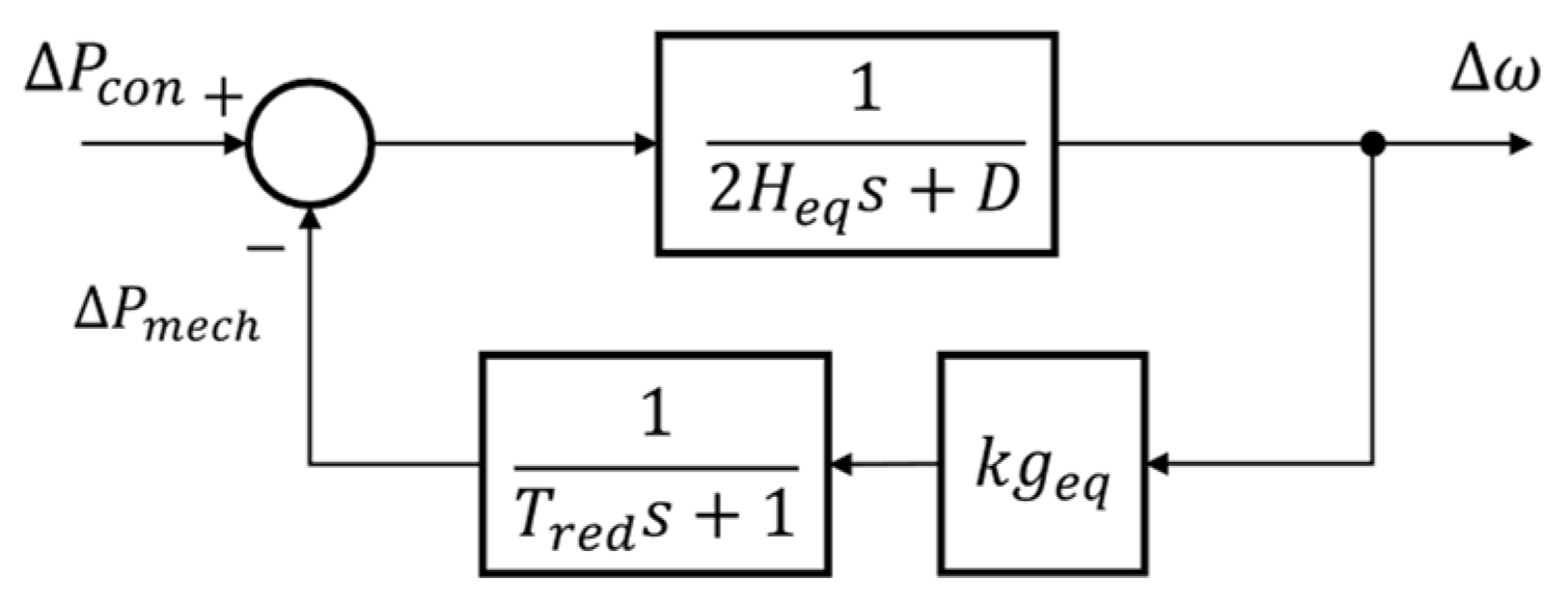
The analytical expression of the frequency was derived using the reduced frequency response (RFR) model, a single-machine frequency response model. This model, which is based on the basic concept of the swing equation, estimates the frequency of the system in response to power imbalances [26,27]. The RFR model uses the equivalent turbine-governor model as a general and simple first-order system and is illustrated in Figure 1 [28].
Studies on inertia constraints have mainly used system frequency response (SFR) models [29,30] based on reheat steam turbines [20,22,24,25]. The RFR model is advantageous as it can cover a wide range of generator types; this benefit is attributed to the usage of a simple turbine-governor model. In addition, as the RFR model minimizes the number of parameters in the turbine-governor model, the number of variables that need to be considered in the linearization process is small, unlike the SFR model. Therefore, the RFR model allows inertia constraints that reflect the load-damping constant to be modeled while still considering all inertia and governor-related variables. If the load-damping constant can be considered as a variable in the inertia constraint, the system inertia and the generator gain can be secured to reflect the different load characteristics in each time interval of the UC.
For the system presented in Figure 1, when the damping ratio is in the range , the analytical expression of the frequency deviation is as follows [28]:
where
is the change in instantaneous generation owing to contingency, is the load-damping constant, is the generator gain of a single machine, is the system inertia, and is the time constant of a single machine.
The analytical expression for the minimum frequency deviation in the RFR model is as follows [28]:
where
In this study, we used the analytical expression for all ranges of from [28] to model the inertia constraints. The analytical expressions for the remaining ranges are omitted.
2.2. Piecewise Linearization Technique for Linearizing the Analytical Expression
The max-affine function-based fitting technique is used for determining the optimal PWL approximation when the number of segments is determined [31]. This technique can yield a PWL approximation for multivariate functions, and a higher linearization accuracy can be achieved by optimizing the determined segments. This technique has been mainly used in studies to model minimum frequency constraints using a single-machine frequency response model [20,24,25].
As reported in [22], applying four variables when linearizing the minimum frequency constraint with this technique is extremely complicated. Therefore, the optimal variables must be determined based on appropriate assumptions.
Among the parameters of the RFR model, is determined by market rules, and is less sensitive to frequency than other parameters [24]. Thus, these two parameters are considered externally determined constants. Therefore, in the proposed average RoCoF constraint and minimum frequency constraint, , , and are determined as variables. Notably, the RFR model minimizes the number of parameters, which allows for the load-damping factor to be included in the variables. The parameters for the max-affine function are calculated as follows:
where is the number of data samples, is the number of segments, , , , are the parameters of the max-affine function, and is the data sample.
2.3. Linearized Inertia Constraint Model
2.3.1. Average Rate of Change of Frequency Constraint Model
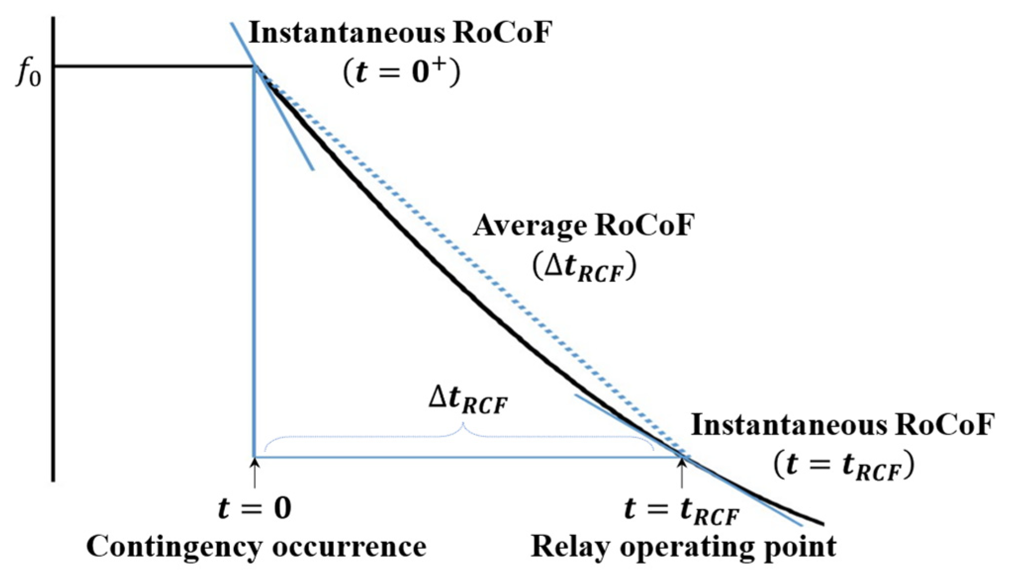
RoCoF protection relays are typically time delay relays. A RoCoF relay will not operate unless a RoCoF above a certain threshold is continuously measured within a set time delay [32]. Figure 2 presents a conceptual illustration of instantaneous RoCoF and average RoCoF. The instantaneous RoCoF is usually the largest at the time of the contingency; thus, considering the behavior of the relay, the RoCoF constraint using the instantaneous RoCoF at that time can conservatively secure system inertia. On the other hand, with the average RoCoF during the time delay of the relay, reasonable system inertia can be secured while preventing relay behavior. In addition, if fast response resources are utilized to support the system inertia, the improvement effect of the RoCoF owing to the frequency responses of these resources is reflected, thereby securing system inertia, which is another potential advantage of this technique [23].
The average RoCoF constraint is modeled using an analytical expression of frequency as follows:
As (11) is a nonlinear constraint, it is modeled as a linear constraint using the PWL technique.
2.3.2. Minimum Frequency Constraint Model
The minimum frequency constraint can be modeled using the minimum frequency deviation magnitude as follows:
The growth of renewable energy, especially solar generation, results in a duck curve in net demand. As the duck curve deepens, the level of net demand can vary widely within a day. The net demand affects the commitment of synchronous units, which can alter the PFR characteristics of the system. Since the PFR characteristics of the system are expressed based on those of a single machine, assuming that the time constant of a single machine is always constant in all time intervals of the UC without considering the system’s characteristics may lead to inefficiencies in terms of securing the inertia and the generator gain.
A typical PSH unit can offer a reserve to the system through governor control and automatic generation control (AGC) only in the generation mode. While in the pumping mode, the PSH unit can create demand to reduce the ramping requirements of the system and provide inertia and reserve through the operation of other synchronous units. To secure reserve and optimize cost, the PSH unit, whose commitment is determined in the UC, is mainly determined to be in pumping mode during periods when net demand is low and is mainly determined to be in generation mode during periods when net demand is high. Therefore, as the net demand level determines the operating status of the PSH units, the minimum frequency constraint is modeled to classify the system according to the net demand level using the operating status of the PSH units as an indicator and to determine the minimum frequency using a different time constant of the single machine in each classified system. The proposed linearized minimum frequency constraint is as follows:
The operating status of the PSH unit is categorized into a generation mode, wherein the PSH unit operates in a generator and a non-generation mode, wherein the PSH unit does not operate as a generator. The minimum frequency constraint is modeled to ensure that the constraints of only one status are valid for each operating status of the PSH units; this approach is based on a binary variable that represents the operating status of all PSH units.
2.3.3. Quasi Steady State Frequency Constraint Model
The quasi steady-state frequency constraint is independent of system inertia and depends solely on the PFR of the system and the characteristics of load changes with respect to frequency changes. Therefore, this constraint is a factor considered in the frequency constraints but is an additional constraint in the inertia constraints. However, from the perspective of stable operation of the system, this constraint can be included in the inertia constraints [9,15]. As this constraint is a linear constraint, it was modeled as follows without any linearization process:
The quasi steady-state frequency constraint is modeled in the same contingency as the minimum frequency constraint.
2.4. Variables for Linearized Inertia Constraints
2.4.1. System Inertia
The system inertia used in the linearized inertia constraint is the system inertia after the contingency. The system inertia is divided into and such that the average RoCoF constraint and the minimum frequency constraint can have different contingencies. The system inertia is modeled to be determined in the UC as indicated in (17) and (18).
System inertia includes the inertia of units in start-up processes and shut-down processes. The start-up processes are the processes in which the unit is connected to the system and increases its power output to reach the minimum power output, and the shut-down processes are the processes in which the unit reduces its power output below the minimum power output to disconnect from the system.
2.4.2. Generator Gain of Single Machine
The generator gain used in the linearized inertia constraints represents the generator gain of the single machine after the contingency. In particular, the generator gain of the single machine is determined by the generator gains of the individual units.
A unit with a high-power output level compared to the maximum power output limit may not be able to provide sufficient PFR according to the predetermined generator gain. If the power output limits of these units are not considered when determining the generator gain of the single machine, then the generator gain of the single machine may be overestimated. Therefore, to determine the generator gain of the single machine, the power output limits of the individual units were considered, and the generator gains of the individual units were recalculated as follows:
To determine the individual generator gains, we compared the generator gain that is calculated assuming the PFRs are provided as total capacities required to increase power outputs of the units to the output limits at the critical quasi steady-state frequency, with the existing inputted generator gains, and choose the lesser of the two values. The redetermined individual generator gains are determined conservatively by using the critical frequency deviation and can be represented as linear constraints. The generator gain of the single machine is determined from the redetermined individual generator gains and is categorized as and to allow for assumed different contingencies depending on the constraints.
2.4.3. Load-Damping Constant
The load-damping constant is independent of the commitment of units. Therefore, the inputted load-damping constant is converted to a form that can be applied to the linearized inertia constraints.
2.5. Time Constant of Single Machine
The frequency sensitivity to the time constant is lower than the frequency sensitivity to other parameters [24]. However, if the time constant set as a constant is not appropriate, it can hinder the linearized inertia constraints from behaving appropriately.
The time constant of the single machine is determined based on the committed units. In large systems, the time constant of the single machine cannot be determined by examining every possible combination of the units. Therefore, in this study, a heuristic approach was used to estimate the time constant of the single machine. The time constant of the single machine is determined by adding a correction constant to the average time constant TAvg of the single machine.
is the average of the time constants of the single machine calculated at the times when the frequency stability problems occurred. Assuming a conservative approach, only the times when stability problems occur are considered, but the average value of the calculated time constants is used instead of the maximum time constant.
The correction constant is applied to compensate for the fitting error [20] of the linearization process and to correct for the error between the frequency calculated by the analytical expression and the actual frequency. Moreover, the correction constant can also serve to ensure the validity of the inertia constraints even when the standard deviation of the time constants derived for the average time constant calculation is large. The correction constant can be determined based on the standard deviation of the time constants; however, deriving the optimal value through iterative calculation is determined to be the most economical approach.
For the minimum frequency constraint, the average constant and the correction constant are each calculated according to the operating status of the PSH units to determine each of the time constants of the single machine. As the average RoCoF is less affected by the PFRs compared to the minimum frequency, we assumed a more efficient approach wherein the number of constraints was minimized by applying a single time constant rather than differentiating the time constant according to the operating status of the PSH units in the average RoCoF constraint.
3. Unit Commitment Model for Linearized Inertia Constraints
3.1. Objective Function
The objective function of UC is to minimize the total system cost, which consists of operating costs, no-load costs, and start-up costs.
3.2. Unit Commitment Constraints
Traditional constraints and the constraints for applying linearized inertia constraints were described.
3.2.1. Power Balance Constraints
The power outputs of renewable energy are assumed to be predetermined.
3.2.2. Power Limit Constraints
The power limit constraints consider the primary and secondary reserves provided by the committed units. In this regard, the primary reserve is defined as the reserve capacity provided by the governor, and the secondary reserve is the reserve capacity provided by the AGC. The secondary reserve is divided into upward secondary reserve, which increases the output power of the unit, and downward secondary reserve, which decreases the output power of the unit.
3.2.3. Ramp Rate Constraints
The ramp rate constraints are reflected in the reserve capacity, and the status of the unit that cannot be start-up/shut-down within a single time interval of UC is considered.
3.2.4. Minimum Up/Down Time Constraints
The minimum up time is the minimum time interval during which the unit must operate continuously at or above the minimum power output limit. The minimum down time is the minimum time interval for the unit to restart after shut-down and includes the time when the unit is operating below the minimum power output limit for the shut-down and start-up processes.
3.2.5. Start-Up/Shut-Down Power Output
We considered the power output of the unit whose start-up time or shut-down time exceeds a single time interval of UC. As adjusting the power output during start-up and shut-down is challenging, a fixed power trajectory is assumed.
3.2.6. Reserve Capacity Constraints
The system is constrained to meet its primary and secondary reserve requirements.
3.2.7. Constraints on Pumped Storage Hydropower Units
PSH units exhibit an energy constraint based on upper reservoir volume.
PSH units are optimized for each unit in the UC. At a certain time, a contradictory state may occur wherein certain PSH units supply energy to the system through generation mode, whereas other PSH units store energy from the system through pumping mode. Therefore, a binary variable representing the overall operating status of all PSH units is introduced to prevent these contradictory states from occurring.
To ensure that the PSH units can operate flexibly and consistently with the net demand level, the stored energy of the PSHs is constrained to half of the maximum storable energy at the start time of the UC.
3.2.8. Binary Variable Constraints
Constraints on the binary variables that represent the operating status of the units.
4. Case Study
To validate the proposed linearized inertia constraints, we compared the results of UC and frequency stability with and without proposed inertia constraints on the systems wherein frequency stability problems occurred owing to low system inertia. Moreover, we examined the efficiency of the proposed inertia constraints compared to the existing inertia constraints.
4.1. Description of System and Premises
A case study was conducted for the South Korean power system in 2030. The system is an isolated system that features a total installed capacity of 20.4 GW of nuclear units and a total installed capacity of 5.5 GW of PSH units in 2030. Table 1 shows the average parameters of the units for each power plant type in the system. The parameters used in the case study are not average parameters but individual parameters for each unit.
The 183 units, excluding 18 nuclear units that cannot provide a frequency response, have the turbine-governor models of PSS/E. Among the units that provide frequency response, 103 combined cycle units have the GAST model, 57 thermal units have the IEEEG1 model, and the remaining 23 hydro units and PSH units have the HYGOV model.
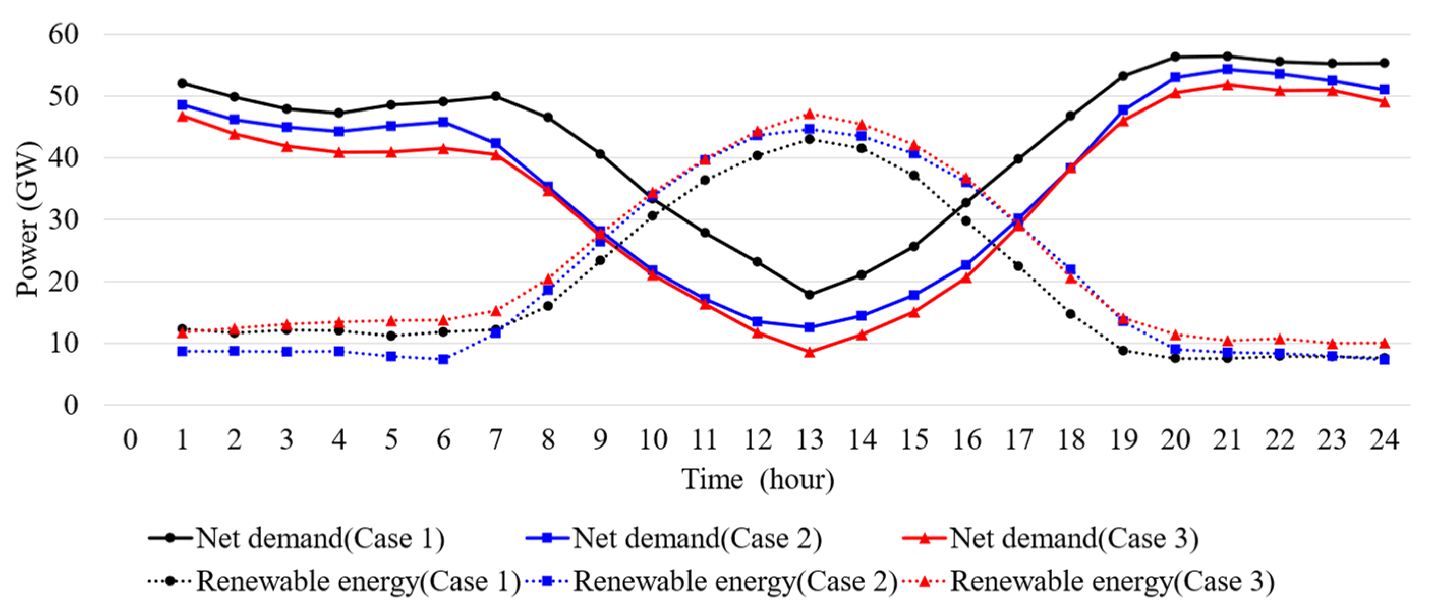
Three cases were selected for the case study based on the lowest net demand level on days when frequency stability problems occur. The net demand and renewable energy of the selected cases are plotted in Figure 3.
The UC is performed by applying five methods of inertia constraints to the selected systems. Method 1 is a conventional method that does not apply inertia constraints. Method 2 is a method that constrains the system inertia to be secured above critical inertia [9,12]. The critical inertia of Method 2 is determined externally by using the method of calculating the instantaneous RoCoF in the contingency.
Method 3 is a boundary constraint method that limits the parameters of the SFR model corresponding to the decision variables to ranges of bounded values [22]. As the methodology for determining the parameters of the SFR model in the actual turbine-governor model is not clear, this method is implemented using the RFR model in this study. The boundary constraints are modeled to constrain the system inertia and the generator gain of the single machine to a range of bounded values. In addition, as it is difficult to extract the boundaries by combining the committed status of all units in large systems such as South Korea, the boundary values that maintain frequency stability are derived through iterative simulations.
Method 4 applies a minimum frequency constraint modeled through a single time constant regardless of the operating status of the PSH units, unlike the proposed inertia constraints. This method is used to validate the proposed minimum frequency constraint, and the rest of the inertia constraints are the same as those used in Method 5, except for the minimum frequency constraint. Method 5 is the proposed linearized inertia constraint method.
Curtailment of renewable energy power is not considered in the UC. This curtailment of power may result in additional commitment of synchronous units. When both inertia constraints and renewable energy curtailment are applied simultaneously, clearly identifying the basis on which the system inertia and PFRs are additionally secured may be difficult.
In particular, regulating the power output of nuclear units during the day is challenging, and these units are mainly operated at maximum power. Therefore, the nuclear units are constrained to be continuously committed at maximum power or continuously shut-down for each unit. For the frequency stability analysis, the nuclear units subject to the contingency are constrained to ensure that they are invariably committed at maximum power.
The RoCoF stability criterion is set to not exceed 0.5 Hz/s for the simultaneous loss of two 1400 MW nuclear units, the units with the largest capacity. The minimum frequency stability criterion is set to not exceed a frequency deviation of 0.3 Hz for the loss of a single 1400 MW nuclear unit, and the quasi steady-state frequency stability criterion is set to not exceed a frequency deviation of 0.2 Hz for the same contingency.
UC was performed on a PC with Intel (R) Core (TM) i5-8400 CPU @ 2.80 GHz, 16 GB RAM using MATLAB R2021a Update 4 with Optimization Toolbox. Frequency simulations were performed in MATLAB R2021a Update 4 using a multi-machine frequency response model with turbine-governor models of PSS/E.
4.2. Frequency Stability Results
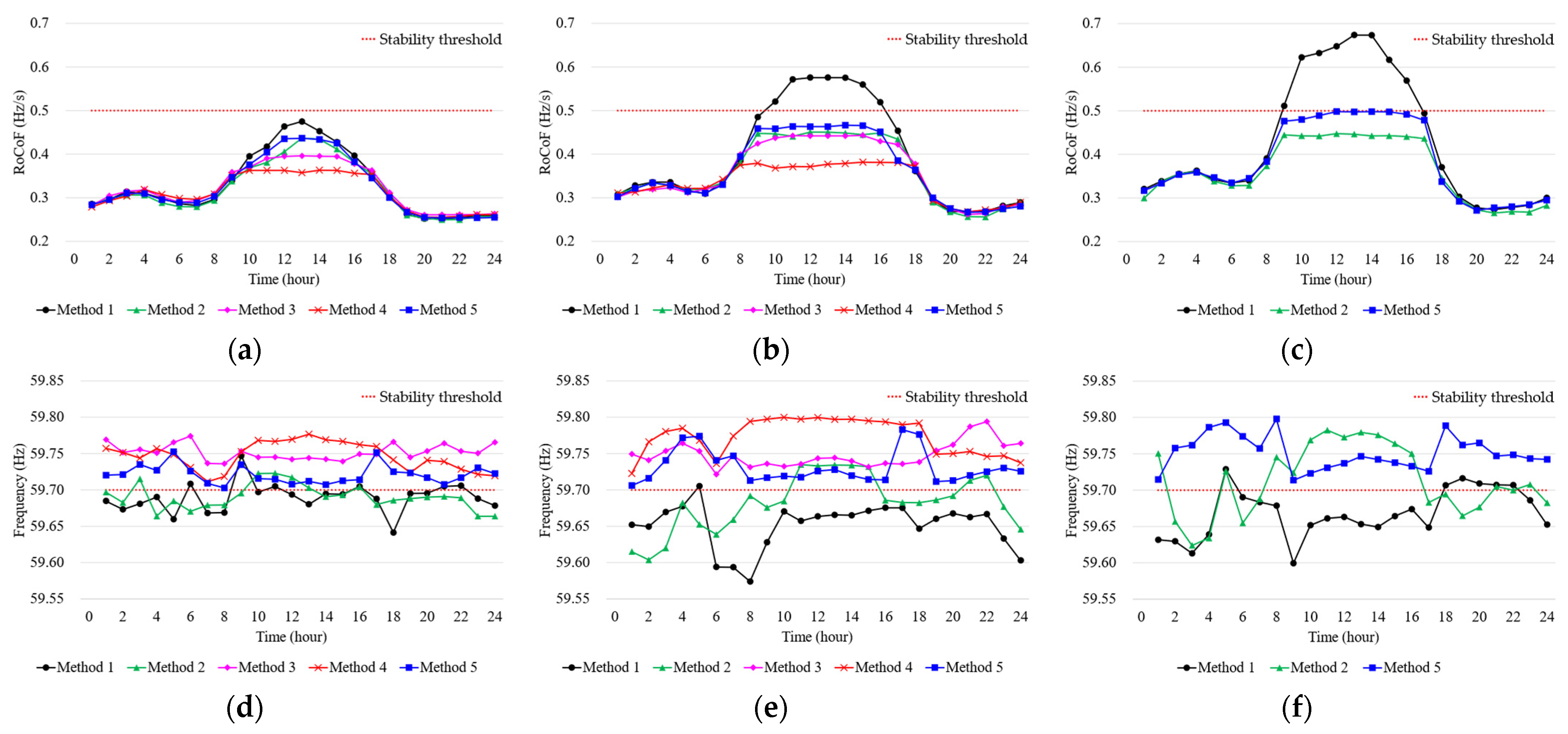
The average RoCoF and minimum frequency for each method in all cases are plotted in Figure 4. The average RoCoF is calculated as the average RoCoF for 0.5 s after the contingency, considering the time delay of the protection relay. The quasi steady-state frequency is independent of the system inertia and is an auxiliary factor of the inertia constraints; in all cases, stability is achieved by securing only the reserve of the existing market rules. Considering this aspect, this result was omitted.
Only the UC with the proposed inertia constraints was able to derive generation mixes that satisfied frequency stability in all cases. Methods 3 and 4 were able to derive generation mixes that satisfied frequency stability in Case 1 and Case 2; however, they were unable to derive feasible solutions in Case 3, which had the lowest net demand. In all cases, the generation mixes of Method 2 were able to achieve the RoCoF stability but did not meet the minimum frequency stability.
4.3. Effects of Linearized Inertia Constraints
4.3.1. Securement of System Inertia
To compare the efficiency of securing system inertia, the average system inertia secured by each method at the times when RoCoF stability problems occurred is listed in Table 2. Methods 2 and 3 secured system inertia above the 168 GWs threshold determined through the instantaneous RoCoF. Method 5, which applied the average RoCoF constraint, was able to secure less system inertia while maintaining RoCoF stability. Although Method 4 applied the average RoCoF constraint, Method 4 secured the most system inertia owing to the minimum frequency constraint. To ensure that the average RoCoF constraint is more efficient at securing system inertia than methods that use instantaneous RoCoF, the efficiency of the minimum frequency constraint must also be guaranteed.
4.3.2. Efficiency of Proposed Minimum Frequency Constraint
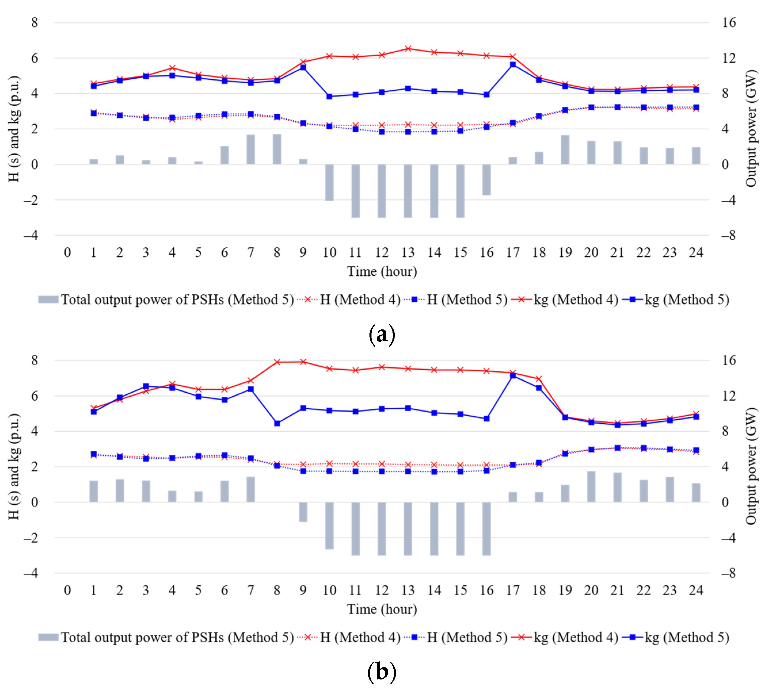
To examine the efficiency of the proposed minimum frequency constraint, the system inertia and the generator gain secured through Method 5 and Method 4 are compared in Figure 5. Method 4 always considers a single time constant, which tends to result in excessively securing the system inertia and the generator gain when the PSH units are operating in a non-generation mode owing to low net demand. In contrast, as Method 5 considers the appropriate time constant according to the operating status of the PSH units, it is more efficient in securing the system inertia and the generator gain while satisfying the minimum frequency stability.
4.3.3. Securement of Generator Gain of the Single Machine
The generator gain of the single machine determines the amount of the PFR provided by the system. The average generator gains obtained for each inertia constraint method in all cases are listed in Table 3. On average, Method 5 resulted in generation mixes that satisfied frequency stability with less secured generator gain than the other methods. Unlike Method 3, Method 5 can determine the appropriate generator gain by considering the system inertia and load-damping constant at each time interval, and unlike Method 4, it is able to avoid excessive securing of the generator gain at certain times.
4.3.4. Acceptance of Inflexible Generation and Total Cost
In each case, the renewable energy power output applied to all methods is identical; thus, the power output of the nuclear units is used to analyze the acceptance of the inflexible generation. The power output of the nuclear units according to each inertia constraint method in all cases is listed in Table 4. The proposed method, Method 5, can accept inflexible generation higher than those of Methods 3 and 4, which satisfied the frequency stability owing to the efficiency of securing the system inertia and the generator gain.
The total system cost for each inertia constraint method in all cases is reported in Table 5. The efficiency of the proposed inertia constraints and the resulting increase in the acceptability of economic and inflexible units allowed for economic generation mixes while still satisfying frequency stability.
4.4. Discussion
The UC with the proposed method was able to secure system inertia and generator gain that satisfied the frequency stability in all cases. The proposed method avoided excessive securing inertia by using the average RoCoF constraint, and the minimum frequency constraint, which was modeled as two different systems depending on the operating status of the PSH, could more suitably reflect the changes in the characteristics of the system to secure efficient inertia and generator gain. The proposed method was more efficient than the conventional methods in terms of securing inertia, securing generator gain, and total system cost; this allowed the derivation of generation mixes that satisfied frequency stability even in Case 3 with a low net demand level.
5. Conclusions
This study presented a novel approach to modeling linearized inertia constraints of generators for frequency stability in the context of UC. The average RoCoF constraint and minimum frequency constraint were modeled using the RFR model, and the load-damping constant was incorporated as a variable of the linearized inertia constraints. Moreover, the minimum frequency constraint was modeled as two different systems depending on the operating state of the PSH. The minimum frequency of each subsystem was determined by its individual time constant. The quasi steady-state frequency constraint was included in the inertia constraints as an auxiliary constraint. We validated the proposed inertia constraints on the 2030 South Korean power system. The UC with the proposed method was able to secure system inertia and generator gain that satisfied the frequency stability. The proposed method was more efficient than the conventional methods in terms of securing system inertia, securing generator gain, and total system cost; this allowed for deriving generation mixes that satisfied frequency stability even in a system with a low net demand level.
The proposed inertia constraint, a method of maintaining frequency stability with only synchronous units in a large isolated system, can be utilized in cases wherein fast response resources are not utilized, or even with their utilization, to conservatively secure system inertia. Future research on inertia constraint should consider the frequency response characteristics of fast response resources and renewable energy generators and the curtailment of renewable energy power output. Finally, future studies should aim to solve large-scale optimization problems that arise owing to increasingly complex operating conditions.
Author Contributions
Conceptualization, S.-E.K. and Y.-H.C.; methodology, S.-E.K.; supervision, Y.-H.C.; writing—original draft preparation, S.-E.K. All authors have read and agreed to the published version of the manuscript.
Funding
This work was supported by the Korea Institute of Energy Technology Evaluation and Planning (KETEP) and the Ministry of Trade, Industry and Energy (MOTIE) of the Republic of Korea (No. 2019371010006B).
Data Availability Statement
The original contributions presented in the study are included in the article, further inquiries can be directed to the corresponding author.
Conflicts of Interest
The authors declare no conflicts of interest.
Nomenclature
| Sets and Indices | |
| Set of time in UC, | |
| Set of synchronous units | |
| Set of PSH units, | |
| Set of tripped units of a contingency for the average RoCoF constraint, | |
| Set of tripped units of a contingency for the minimum frequency constraint, | |
| Set of segments of the average RoCoF constraint/minimum frequency constraint | |
| Parameters | |
| System nominal frequency [Hz] | |
| RoCoF limit [Hz/s] | |
| Minimum frequency deviation limit [Hz] | |
| Quasi steady-state frequency deviation limit [Hz] | |
| Parameters for the average RoCoF constraint | |
| Parameters for the average RoCoF constraint | |
| Parameters for the minimum frequency constraint (generation mode of PSH) | |
| Parameters for the minimum frequency constraint (non-generation mode of PSH) | |
| Inertia constant of unit g [s] | |
| Generator gain of unit g [p.u.] | |
| Machine base of unit g [MVA] | |
| System base [MVA] | |
| Power output of renewable energy/load on the system [MW] | |
| Load-damping constant based on [p.u.] | |
| Operating cost/no-load cost/start-up cost of unit g [USD/MWh] | |
| Maximum/minimum power output limit of unit g [MW] | |
| Maximum/minimum pumping power input of PSH unit g [MW] | |
| Ramp-up/-down rate of unit g [MW/h] | |
| Start-up/shut-down ramp rate of unit g [MW/h] | |
| Start-up/shut-down time of unit g [h] | |
| Minimum up/down time of unit g [h] | |
| Maximum primary reserve of unit g [MW] | |
| Maximum upward/downward secondary reserve of unit g [MW] | |
| Requirement of primary reserve of the system [MW] | |
| Requirement of upward/downward secondary reserve of the system [MW] | |
| Maximum storable energy for PSH unit g [MWh] | |
| Pumping efficiency of PSH unit g | |
| Variables | |
| System inertia constant of the average RoCoF constraint/the minimum frequency constraint [p.u.] | |
| Generator gain of the single machine of the average RoCoF constraint/the minimum frequency constraint [p.u.] | |
| Generator gain of unit g considering generation limits [p.u.] | |
| Power output/pumping power input of unit g/PSH unit g [MW] | |
| Start-up/shut-down power output of unit g [MW] | |
| Primary/upward secondary/downward secondary reserve of unit g [MW] | |
| Energy stored in PSH unit g [MWh] | |
| Binary variable representing commitment status of unit g | |
| Binary variable representing the operating status of PSH unit g (1 if in pumping mode and 0 if not in pumping mode) | |
| Binary variable representing start-up/shut-down status of unit g (1 if the end of start-up process/the start of the shut-down process) | |
| Binary variable representing start-up/shut-down processes of unit g (1 if while in start-up process/shut-down process) | |
| Binary variable representing generation/pumping mode of all PSH units (1 if in generation/pumping mode) | |
References
- Ørum, E.; Kuivaniemi, M.; Laasonen, M.; Bruseth, A.I.; Jansson, E.A.; Danell, A.; Elkington, K.; Modig, N. Future System Inertia; ENTSOE: Brussels, Belgium, 2018. [Google Scholar]
- ENTSOE subgroup system protection inertia TF. Inertia and Rate of Change of Frequency (RoCoF); ENTSOE: Brussels, Belgium, 2020. [Google Scholar]
- Johnson, S.C.; Papageorgiou, D.J.; Mallapragada, D.S.; Deetjen, T.A.; Rhodes, J.D.; Webber, M.E. Evaluating rotational inertia as a component of grid reliability with high penetrations of variable renewable energy. Energy 2019, 180, 258–271. [Google Scholar] [CrossRef]
- Mehigan, L.; Al Kez, D.; Collins, S.; Foley, A.; Ó’Gallachóir, B.; Deane, P. Renewables in the European power system and the impact on system rotational inertia. Energy 2020, 203, 117776. [Google Scholar] [CrossRef]
- Villamor, L.V.; Avagyan, V.; Chalmers, H. Opportunities for reducing curtailment of wind energy in the future electricity systems: Insights from modelling analysis of Great Britain. Energy 2020, 195, 116777. [Google Scholar] [CrossRef]
- Kerdphol, T.; Rahman, F.S.; Watanabe, M.; Mitani, Y.; Turschner, D.; Beck, H. Enhanced virtual inertia control based on derivative technique to emulate simultaneous inertia and damping properties for microgrid frequency regulation. IEEE Access 2019, 7, 14422–14433. [Google Scholar] [CrossRef]
- Du, P.; Mago, N.V.; Li, W.; Sharma, S.; Hu, Q.; Ding, T. New ancillary service market for ERCOT. IEEE Access 2020, 8, 178391–178401. [Google Scholar] [CrossRef]
- Chamorro, H.R.; Sevilla, F.R.S.; Gonzalez-Longatt, F.; Rouzbehi, K.; Chavez, H.; Sood, V.K. Innovative primary frequency control in low-inertia power systems based on wide-area RoCoF sharing. IET Energy Syst. Integr. 2020, 2, 151–160. [Google Scholar] [CrossRef]
- Mosca, C.; Bompard, E.; Chicco, G.; Aluisio, B.; Migliori, M.; Vergine, C.; Cuccia, P. Technical and economic impact of the inertia constraints on power plant unit commitment. IEEE Open Access J. Power Energy 2020, 7, 441–452. [Google Scholar] [CrossRef]
- Schipper, J.; Wood, A.; Edwards, C. Optimizing instantaneous and ramping reserves with different response speeds for contingencies—Part I: Methodology. IEEE Trans. Power Syst. 2020, 35, 3953–3960. [Google Scholar] [CrossRef]
- Muzhikyan, A.; Mezher, T.; Farid, A.M. Power system enterprise control with inertial response procurement. IEEE Trans. Power Syst. 2018, 33, 3735–3744. [Google Scholar] [CrossRef]
- Daly, P.; Flynn, D.; Cunniffe, N. Inertia considerations within unit commitment and economic dispatch for systems with high non-synchronous penetrations. In Proceedings of the IEEE Eindhoven Powertech, Eindhoven, The Netherlands, 29 June–2 July 2015; pp. 1–6. [Google Scholar]
- Banik, S.; Sakib, M.S.; Chowdhury, S.; Masood, N.A. Inertia constrained economic dispatch in a renewable dominated power system. In Proceedings of the IEEE PES Innovative Smart Grid Technologies Conference—Latin America (ISGT Latin America), Lima, Peru, 15–17 September 2021; pp. 1–5. [Google Scholar]
- Helistö, N.; Kiviluoma, J.; Ikäheimo, J.; Rasku, T.; Rinne, E.; O’Dwyer, C.; Li, R.; Flynn, D. Backbone—An adaptable energy systems modelling framework. Energies 2019, 12, 3388. [Google Scholar] [CrossRef]
- Teng, F.; Trovato, V.; Strbac, G. Stochastic scheduling with inertia-dependent fast frequency response requirements. IEEE Trans. Power Syst. 2016, 31, 1557–1566. [Google Scholar] [CrossRef]
- Badesa, L.; Teng, F.; Strbac, G. Simultaneous scheduling of multiple frequency services in stochastic unit commitment. IEEE Trans. Power Syst. 2019, 34, 3858–3868. [Google Scholar] [CrossRef]
- Badesa, L.; Teng, F.; Strbac, G. Conditions for regional frequency stability in power system scheduling—Part I: Theory. IEEE Trans. Power Syst. 2021, 36, 5558–5566. [Google Scholar] [CrossRef]
- Badesa, L.; Teng, F.; Strbac, G. Conditions for regional frequency stability in power system scheduling—Part II: Application to unit commitment. IEEE Trans. Power Syst. 2021, 36, 5567–5577. [Google Scholar] [CrossRef]
- Wen, Y.; Li, W.; Huang, G.; Liu, X. Frequency dynamics constrained unit commitment with battery energy storage. IEEE Trans. Power Syst. 2016, 31, 5115–5125. [Google Scholar] [CrossRef]
- Zhang, C.; Liu, L.; Cheng, H.; Liu, D.; Zhang, J.; Li, G. Frequency-constrained co-planning of generation and energy storage with high-penetration renewable energy. J. Mod. Power Syst. Clean Energy 2021, 9, 760–775. [Google Scholar] [CrossRef]
- Javadi, M.; Gong, Y.; Chung, C.Y. Frequency stability constrained microgrid scheduling considering seamless islanding. IEEE Trans. Power Syst. 2022, 37, 306–316. [Google Scholar] [CrossRef]
- Paturet, M.; Markovic, U.; Delikaraoglou, S.; Vrettos, E.; Aristidou, P.; Hug, G. Stochastic unit commitment in low-inertia grids. IEEE Trans. Power Syst. 2020, 35, 3448–3458. [Google Scholar] [CrossRef]
- Trovato, V.; Bialecki, A.; Dallagi, A. Unit commitment with inertia-dependent and multispeed allocation of frequency response services. IEEE Trans. Power Syst. 2019, 34, 1537–1548. [Google Scholar] [CrossRef]
- Ahmadi, H.; Ghasemi, H. Security-constrained unit commitment with linearized system frequency limit constraints. IEEE Trans. Power Syst. 2014, 29, 1536–1545. [Google Scholar] [CrossRef]
- Zhang, Z.; Du, E.; Teng, F.; Zhang, N.; Kang, C. Modeling frequency dynamics in unit commitment with a high share of renewable energy. IEEE Trans. Power Syst. 2020, 35, 4383–4395. [Google Scholar] [CrossRef]
- Kundur, P. Power System Stability and Control; McGraw-Hill: New York, NY, USA, 1994. [Google Scholar]
- Wood, A.J.; Wollenberg, B.F.; Sheblé, G.B. Power Generation, Operation, and Control, 3rd ed.; John Wiley & Sons: Hoboken, NJ, USA, 2015. [Google Scholar]
- Kim, S.; Chun, Y. Single-machine frequency model and parameter identification for inertial constraints in unit commitment. Energies 2021, 14, 5961. [Google Scholar] [CrossRef]
- Anderson, P.M.; Mirheydar, M. A low-order system frequency response model. IEEE Trans. Power Syst. 1990, 5, 720–729. [Google Scholar] [CrossRef]
- Shi, Q.; Li, F.; Cui, H. Analytical method to aggregate multi-machine SFR model with applications in power system dynamic studies. IEEE Trans. Power Syst. 2018, 33, 6355–6367. [Google Scholar] [CrossRef]
- Magnani, A.; Boyd, S.P. Convex piecewise-linear fitting. Optim. Eng. 2009, 10, 1–17. [Google Scholar] [CrossRef]
- Operations directorate of ENA. Engineering Recommendation G59 Issue 3 Amendment 7; ENA: London, UK, 2019. [Google Scholar]
Figure 1.
Reduced frequency response (RFR) model.

Figure 2.
Instantaneous RoCoF and average RoCoF conceptual illustration.

Figure 3.
Net demand and renewable energy output of the case system.

Figure 4.
Frequency stability results for each method. (a) Average RoCoF of Case 1; (b) Average RoCoF of Case 2; (c) Average RoCoF of Case 3; (d) Minimum frequency of Case 1; (e) Minimum frequency of Case 2; (f) Minimum frequency of Case 3.
Figure 4.
Frequency stability results for each method. (a) Average RoCoF of Case 1; (b) Average RoCoF of Case 2; (c) Average RoCoF of Case 3; (d) Minimum frequency of Case 1; (e) Minimum frequency of Case 2; (f) Minimum frequency of Case 3.

Figure 5.
System inertia and generator gain of the single machine by Method 4 and Method 5. (a) Case 1 system; (b) Case 2 system.
Figure 5.
System inertia and generator gain of the single machine by Method 4 and Method 5. (a) Case 1 system; (b) Case 2 system.


Table 1.
Average parameters of the units for each power plant type in the system.
| Combined Cycle | Thermal Power | Nuclear Power | Hydroelectric Power | Pumped Storage Hydropower | |
|---|---|---|---|---|---|
| Total capacity [MW] | 47,953 | 37,871 | 20,400 | 1582 | 5500 |
| Number of units [EA] | 103 | 57 | 18 | 15 | 8 |
| Operating cost [USD/MWh] | 67 | 37 | 4 | 0 | 0 |
| No-load cost [USD] | 2766 | 3392 | 433 | 0 | 0 |
| Start-up cost [USD] | 2808 | 35,162 | - | 0 | 0 |
| Ramp rate [MW/min] | 21.2 | 16.7 | - | 31.8 | 205.6 |
| Minimum up time [h] | 4.1 | 7.8 | - | 0.5 | 0.5 |
| Minimum down time [h] | 3.5 | 13.7 | - | 0.5 | 0.6 |
| Inertia constant [s] | 5.15 | 3.99 | 4.99 | 3.71 | 4.93 |
| Generator gain [p.u.] | 13.82 | 15.39 | - | 21.85 | 24.93 |
Table 2.
Average system inertia at the times when the RoCoF stability problems occurred.
| Method 1 (GWs) | Method 2 (GWs) | Method 3 (GWs) | Method 4 (GWs) | Method 5 (GWs) | |
|---|---|---|---|---|---|
| Case 2 | 133 | 170 | 173 | 203 | 164 |
| Case 3 | 119 | 170 | - | - | 153 |
Table 3.
Average generator gains for each method in all cases.
| Method 1 (p.u.) | Method 2 (p.u.) | Method 3 (p.u.) | Method 4 (p.u.) | Method 5 (p.u.) | |
|---|---|---|---|---|---|
| Case 1 | 3.43 | 3.49 | 5.50 | 5.24 | 4.47 |
| Case 2 | 3.37 | 3.75 | 5.55 | 6.43 | 5.36 |
| Case 3 | 3.31 | 3.86 | - | - | 5.71 |
Table 4.
Nuclear unit power output for each method in all cases.
| Method 1 (GW) | Method 2 (GW) | Method 3 (GW) | Method 4 (GW) | Method 5 (GW) | |
|---|---|---|---|---|---|
| Case 1 | 15.6 | 14.6 | 12.2 | 10.2 | 14.2 |
| Case 2 | 10.2 | 7.2 | 6.2 | 3.8 | 7.2 |
| Case 3 | 5.8 | 2.8 | - | - | 2.8 |
Table 5.
Total system cost for each method in all cases.
| Method 1 (MUSD) | Method 2 (MUSD) | Method 3 (MUSD) | Method 4 (MUSD) | Method 5 (MUSD) | |
|---|---|---|---|---|---|
| Case 1 | 30.6 | 31.7 | 33.0 | 34.9 | 31.5 |
| Case 2 | 29.0 | 32.1 | 32.6 | 35.1 | 31.7 |
| Case 3 | 31.5 | 36.5 | - | - | 34.1 |
Disclaimer/Publisher’s Note: The statements, opinions and data contained in all publications are solely those of the individual author(s) and contributor(s) and not of MDPI and/or the editor(s). MDPI and/or the editor(s) disclaim responsibility for any injury to people or property resulting from any ideas, methods, instructions or products referred to in the content. |
© 2024 by the authors. Licensee MDPI, Basel, Switzerland. This article is an open access article distributed under the terms and conditions of the Creative Commons Attribution (CC BY) license (https://creativecommons.org/licenses/by/4.0/).
Share and Cite
MDPI and ACS Style
Kim, S.-E.; Chun, Y.-H. Modeling of Linearized Generator Inertia Constraints for Unit Commitment. Energies 2024, 17, 1120. https://doi.org/10.3390/en17051120
AMA Style
Kim S-E, Chun Y-H. Modeling of Linearized Generator Inertia Constraints for Unit Commitment. Energies. 2024; 17(5):1120. https://doi.org/10.3390/en17051120
Chicago/Turabian StyleKim, Sung-Eun, and Yeong-Han Chun. 2024. "Modeling of Linearized Generator Inertia Constraints for Unit Commitment" Energies 17, no. 5: 1120. https://doi.org/10.3390/en17051120
Note that from the first issue of 2016, this journal uses article numbers instead of page numbers. See further details here.