Numerical Methods to Evaluate Hyperelastic Transducers: Hexagonal Distributed Embedded Energy Converters


National Renewable Energy Laboratory, 15013 Denver West Parkway, Golden, CO 80401, USA
*
Author to whom correspondence should be addressed.
Energies 2023, 16(24), 8100; https://doi.org/10.3390/en16248100
Submission received: 19 October 2023
/
Revised: 6 December 2023
/
Accepted: 12 December 2023
/
Published: 16 December 2023
(This article belongs to the Section F3: Power Electronics)
Abstract
:Hexagonal distributed embedded energy converters, also known as hexDEECs, are centimeter-scale energy transducers that leverage variable capacitance to generate electricity when their hyperelastic structure is dynamically deformed. To better understand, characterize, and optimize hexDEEC designs, a series of numerical methods and techniques were developed to model the hyperelastic mechanics of hexDEECs, electrostatic properties, and electricity generation characteristics. The numerical methods developed for the hyperelastic structural analysis were corroborated by empirical results from another study, and the models and equations for capacitance, electrostatic forces, and electrical potential energy were derived from fundamental electrostatic equations. These methods and techniques were implemented within the STAR-CCM+ multiphysics software Version 2020.3 (15.06.008) environment. Results from this analysis revealed methodologies and techniques necessary to model the energy converters, which will enable future exploration and optimization of more specific designs and corresponding applications.
Keywords:
energy transducer; numerical modeling; multiphysics modeling; hexDEEC; hexagonal distributed embedded energy converter; metamaterials; hyperelasticity; DEEC-Tec; distributed embedded energy converter technologies; hyperelastic; variable capacitance; variable capacitance generators; STAR-CCM+; electrostatic; soft-robotics1. Introduction
Hexagonal distributed embedded energy converters (hexDEECs) are a new type of energy transducer that leverage variable capacitance to convert the dynamic deformations of their hyperelastic structure into electricity—as proposed by the National Renewable Energy Laboratory’s (NREL’s) patent: Electric Machines as Motors and Power Generators [1]. Figure 1 provides an overview of an individual hexDEEC, showing the energy transducer’s hyperelastic hexagonal housing, electrode placement, and the gap between positively charged and negatively charged electrodes. The hyperelastic housing is composed of a silicone elastomer, such as Smooth-Sil 950 silicone rubber. Notable features of the silicone elastomer and the reason for its selection as a hexDEEC housing include: (i) less pronounced filler-filler and filler-polymer interaction (minimizing the Mullins-effect/stress-softening); high-dimensional stability (minimal creep deformations) under loading; exhibits good abrasion resistance; can directly withstand wide ranges of temperatures and UV radiation; highly repeatable cyclic loading characteristics; good dielectric properties; and readily adaptable manufacturing processes (e.g., able to vary Shore hardness per a specific hexDEEC application) [2,3,4,5,6,7,8,9,10,11,12,13]. Additionally, silicone elastomers experience significantly lower viscous losses than those elastomers made of acrylics; meaning they can withstand higher frequencies of actuation with lower losses and heat generation than most other materials used in variable capacitance energy harvesting [3,4,5,6,9,14]. Note that this technology needs to survive multiple loading cycles since a hexDEEC fundamentally uses those cycles to harvest and generate energy (as shown in Figure 2). Additionally, compliant electrodes will be used for this design, as is the case for other silicone elastomer-based variable capacitance energy harvesters [9,15,16,17,18,19,20,21]. These compliant electrodes are typically made of various carbon particles in polymer binders, such as carbon grease, or patterned or corrugated metal coatings such as corrugated silver [9,15,21].
A multitude of these small energy generators can be woven together to form larger “metamaterial” frameworks, see Figure 3. As a result, hexDEECs are a form of distributed embedded energy converter technologies (DEEC-Tec), characterized by using many small energy converters that can be distributed, embedded, and/or interconnected to form overall larger energy conversion structures. Potential hexDEEC applications could include, but are not limited to, marine renewable energy conversion, roadway vibrations, building oscillations, or any other dynamically fluctuating structure. Thus, hexDEECs not only represent a fundamentally new type of energy transducer, but they also directly facilitate the advancement of other domains of energy conversion. Indeed, hexDEECs are relatively low-cost, non-toxic, and composed of easily accessible materials (no rare earth materials) and could likely have higher energy densities than those of piezoelectric or electromagnetic energy transducer systems [15,20].
The mechanical-to-electrical conversion cycle of the hexDEEC is shown in Figure 2. First (step 1), the device is pulled in tension, increasing its strain and deforming its internal arrangement of electrode plates such that the original hexagonal capacitor flattens into a thin rectangular capacitor [15,18,20]. Once stretched (step 2), an electrical charge is added to the electrode surfaces via pre-charge circuitry—positive charge is applied to the top three electrode plates, and negative charge is applied to the bottom three electrode plates. These charges generate attractive forces and subsequent Maxwell stresses that aim to keep the hexDEEC in this flattened state [15,18,20]. Once the externally applied tension is removed (step 3), the elastic forces generated by the hexDEEC’s hyperelastic housing oppose the coulombic forces generated by the oppositely charged electrodes and bring the structure back to its original relaxed state [18]. To convert the stored elastic energy in the structure to electrical energy during this step, the charge, voltage, and/or electric field can be held constant by the circuit [15,18,20]. The overall energy gain is dependent upon which of these variables is kept constant, but since the constant voltage cycle requires the least complex energy-harvesting control circuit, this cycle was chosen for the numerical techniques developed and analysis of this work’s hexDEEC design [15,18,20]. Finally, (step 4), the charge is removed from the hexDEEC until it is stretched again and repeats its energy-harvesting cycle [15,18,20].
The following sections detail the research and development of analytical and numerical techniques for analyzing a generic hexDEEC. The implementation of these methods occurs within the multiphysics framework provided by the STAR-CCM+ software environment. This work not only analyzes the capacitance, electrostatic forces, and energy produced by the general hexDEEC design but also outlines methodologies required for modeling hyperelastic materials in STAR-CCM+—outcomes that were validated using empirical results from literature (see [22]). Of particular interest is the software’s ability to incorporate a multitude of physics models with high-performance scalable computation, both in terms of user-developed models (such as those made to incorporate the electrostatic features of the transducer) and also STAR-CCM+’s “out-of-the-box” physics models (such as solid stress, fluid-structure interaction, and electricity-plus-magnetism models). Thus, not only do STAR-CCM+ features enable analyses of individual hexDEECs undergoing uniaxial loading, which is central to this work, but STAR-CCM+ could also enable complex models of multi-axial loadings acting upon woven hexDEEC metamaterials (see Figure 3).
Section 2 describes the derived equations used to determine the capacitance and electrostatic forces on the general hexDEEC design in terms of a constant applied voltage and the transducer’s instantaneous shape. Section 2 also presents the numerical methods used to determine a hexDEEC’s deformation under operating conditions. Section 3 details the analytical and numerical results of the study and verifies the approach used to model a hexDEEC’s hyperelastic characteristics against research conducted by Viljoen [22]. Likewise, Section 3 also describes the findings obtained from the analysis of the hexDEEC’s potential energy production while under tensile loading. Section 4 discusses the results of the analysis and details how the work can be used to advance the continued development of this technology and other potential types of energy transducers based on hexDEECs. Lastly, Section 5 elaborates on the potential avenues of hexDEEC and hexDEEC metamaterial advancements, indicating future pathways for ongoing hexDEEC-based research, development, and corresponding applications.
2. Materials and Methods
To determine the energy that could be generated by a hexDEEC, analytical equations were first developed to find the capacitance of the unique hexagonal-shaped capacitor as described in Section 2.1. The equations developed in this section were used to determine the electrical potential energy and electrostatic forces given the shape of a hexagonal capacitor. Next, it was necessary to understand how the dimensions of the capacitor change due to the deformation of the hexDEEC’s hyperelastic housing under tension. This required identifying a material model for the hyperelastic housing, which was facilitated by an empirical analysis from the literature [22] and determined material models for the specific material planned to be used to manufacture hexDEECs, as described in Section 2.2. In Section 2.3, the models from the literature were recreated in STAR-CCM+ to determine methodologies specific to this software that can accurately represent the results of the prior study [22], which did not use this software. Once these methods were determined and validated, they were then used to model the hexDEECs, as described in Section 2.3. The deformation of a hexDEEC’s housing was then combined with the analytical electrostatic equations to determine the potential energy that could be generated by a hexDEEC.
Note that for this study, the electrodes were considered compliant and idealized, so that they had negligible electrical resistance and mechanical stiffness along with being perfect conductors, as has been done previously in other modeling studies for silicone elastomer-based variable capacitance energy harvesters [19]. As a result, the electrodes were assumed to be perfect conductors and did not affect the mechanics of the hyperelastic silicone housing. However, this simplification is not fully accurate since the compliant electrodes used for similar transducers can have high resistance, damage easily, high stiffness, unevenly distribute charge, impose stress concentrations, and have nonuniform coverage at high strains which can reduce the performance and potential lifetime of the device [15,16,17,21]. The properties of these compliant electrodes vary with the material chosen, where the more commonly used carbon-based electrodes tend to have a low impact on stiffness but have high resistance, and the metallic-based electrodes have high conductivity but high stiffness [21]. Additionally, the integrity of the compliant electrodes can be negatively impacted by humidity, strong electric fields, and high strains [15]. Though novel materials are being developed that can have both low stiffness and high conductivity, which more closely represent the properties of the electrodes modeled in this study, they are still in early development [21]. While an idealization was used for the electrodes modeled for the hexDEEC, future studies can evaluate the impacts of the electrode material chosen on the electrostatic and hyperelastic physics assessed in this study.
2.1. Deriving Analytical Electrostatic Equations for HexDEEC
To determine the potential energy of a hexDEEC (or any hexagonal capacitor), a rigorous process was undertaken, relying on the principles of fundamental electrostatics theory. These calculations, outlined in Section 2.1.1 and Section 2.1.2, involve deriving equations that encompass the spatial geometry, dielectric properties, and charge distribution, thereby providing a comprehensive understanding of the energy stored within these types of energy transducers.
2.1.1. Electric Potential Energy
HexDEECs rely on variable capacitance to produce electricity. The simplest variable capacitor is generally represented as two parallel conducting plates, where one holds positive charges while the other holds negative charges. The capacitance between these plates, C, is defined by the charge stored between them, or the ratio of the magnitude of charge on each plate, Q, to the voltage applied to the plates, V, which, using Maxwell’s equations, simplifies to a ratio between, the permittivity of a vacuum, , dielectric constant, , area of the plates, A, and the distance between the plates, z:
The resulting electrical potential energy of this system, U, is dependent on the work required to keep the charges separated and is influenced by the voltage, charge difference, and resulting capacitance of the system:
The capacitance and energy of a capacitor can be increased by inserting a dielectric material that increases the effective permittivity between the plates by multiplying it by a corresponding dielectric constant, . Note that a dielectric with a factor greater than 1 is polarized by the electric field of the capacitor, which attracts more charge to the electrode plates.
Note that, in this work, the dielectric constant will be assumed as 1; this being the approximate permittivity of air with air being the weakest dielectric between a hexDEEC’s electrode plates (as opposed to any other dielectric and, thus, corresponding permittivity.
Variable capacitors generate energy after their charge, voltage, or electric field strength is altered as a result of experiencing an externally inputted alteration—for instance, a force that pushes the plates closer together and then releases them back to their original position—while charge, voltage, or electric field strength is maintained [15,18,20]. Note that the choice between charge, voltage, or electric field strength—to be maintained throughout the cycle—impacts the overall energy gain and has practical implications such as increasing the complexity of the power-electronic control systems in the transducer’s energy-harvesting circuitry [15,18,20]. In this regard, constant voltage cycles have the most straightforward power-electronic circuit design and is therefore the method assumed for this work’s initial evaluation [15].
Nonetheless, hexDEECs do not rely solely on parallel plates to generate electricity; they also contain two pairs of angled plates. The upper three and bottom three plates are kept at the same voltage so they can be considered as capacitors in parallel, where the first and third capacitors contain angled plates while the second capacitor is a classic parallel plate capacitor. Because these capacitors are in parallel, their capacitances simply add such that the total capacitance of the hexagonal capacitor is .
The capacitance of the angled plates can be determined by breaking them into infinitesimally thin parallel plate capacitors in parallel (Figure 4). Each of these capacitors has a capacitance of
Since the distance between the plates varies with length rather than width, the width of each plate, W, is constant. Therefore, the area of each infinitesimal plate is
Note that an individual hexDEEC is assumed to be exceptionally smaller than its corresponding overall “metamaterial hexDEEC fabric”—where such a metamaterial would be made from the large aggregation (thousands, millions, etc.) of individual hexDEECs. To help visualize such a metamaterial fabric, see Figure 3). Emerging from this disproportionate difference in scale—an individual scale vs. a hexDEEC metamaterial scale—is the assumption that while the much larger metamaterial hexDEEC fabric could directly experience large three-dimensional deformations (bending, twisting, etc.), the individual hexDEECs making up that fabric would, in large part, not directly “see/experience” such three-dimensional deformations. Rather, at the scale of an individual hexDEEC, those larger three-dimensional metamaterial hexDEEC fabric deformations would be (can be assumed to be dispersed as) two-dimensional axial loads along any given individual hexDEEC’s characteristic length. Moreover, note that the hexDEEC’s electrode plates for this study were split into thin strips rather than small cubes with infinitesimal widths as well as lengths as a means to facilitate this two-dimensional approximation/assumption. The approximation used in this work, therefore, effectively assumes that the electrode plate surfaces remain flat. Nonetheless, in future work, there will be further investigation into the effects of directly twisting and bending larger individual hexDEECs; where a hexDEEC’s corresponding electrode surfaces can no longer be assumed to be flat with the analysis, in that case, discretizing the electrodes into plates with both infinitesimal widths as well as lengths.
The distance between each infinitesimally thin strip can be determined by bisecting the angle between the two slanted plates, , and examining the distance between the two plates at the edges of their length. At their closest, the plates are separated by , and at their furthest, they are separated by . If a right triangle is made connecting these points, then the height of this triangle will be and its length will be (Figure 5).
Since this relationship is maintained for the progressive capacitors, can be determined as follows:
The capacitance of the slanted plates can then be determined via the integration below, using the definition for from Equation (7):
The result from Equation (8) can then be further simplified using the relationship between and from Equation (6):
Since both capacitors 1 and 3 are angled, their capacitance is equivalent to the result of Equation (9):
Capacitor 2, with a width equal to the slanted plates and a length of , has a capacitance of:
Therefore, the total capacitance of the hexDEEC is
where W is the width of each plate, is the length of the middle plates, is the distance between the middle plates, is the distance between the side plates at their most distal edge, and is half of the angle between the slanted plates (Figure 5). Knowing , the potential energy in the hexDEEC can be calculated as
The potential energy gain and resulting energy that can be harvested by a hexDEEC is therefore dependent on the geometry and orientation of its plates. Note that there could be some electrical potential energy in the hyperelastic housing itself; largely due to polarization. However, this energy is considered negligible when compared to the exceptionally large (1 kilovolt or higher) pre-charge voltage between a hexDEEC’s electrodes. Thus, electric potential energy with the hexDEEC silicon elastomer housing, itself, is asserted to have negligible effects upon the overall performance characteristics of a hexDEEC—that native elastomer electric potential energy is approximated to be zero in this study.
2.1.2. Electrostatic Force
Due to the applied voltage difference on the plates and the resulting electric field, there is an attracting force between the upper and lower plates. For a parallel plate capacitor, the electric force () can be determined by equating the work done to separate the plates at a certain distance (d) to the electric potential energy of the system:
and
The force on each of the flat parallel plates in the middle of the hexDEEC, , is equivalent to half of the electric force:
The force on each of the slanted plates can be determined similarly to finding their capacitance, where
and
2.2. Hyperelastic Material Models for HexDEEC Housing
Since a material with hyperelastic properties will be used for the housing of the electrodes, the finite element analysis software STAR-CCM+ was used to understand how the hexDEEC would deform under biaxial tensile loads. Additionally, this software will be useful in future studies for analyzing the deformation of a multitude of interconnected hexDEECs. The material chosen for this analysis was a common silicone rubber referred to as Smooth-Sil 950, whose material properties were analyzed in detail by Viljoen in their master’s thesis [22]. Note that while Smooth-Sil 950 and other silicone rubbers have both hyperelastic and viscoelastic properties, this analysis will focus on modeling the hyperelastic properties of this material as the effects of viscoelasticity (and corresponding viscous losses) are less significant for silicone elastomers when compared to those other commonly used materials used for variable capacitance-based energy harvesters, such as acrylic-based dielectric elastomer generators [2,3,4,5,6,7,8,9,23,24]. Thus, in large part, a hexDEEC’s performance is not as strongly defined by any viscoelastic effects of this silicone elastomer housing while its hyperelastic housing does dominate a hexDEEC’s elastic behavior; especially in terms of the operational theory of both an individual hexDEEC and, especially, within the context of a hexDEEC-based metamaterial. Nonetheless, future research may delve into the effects of viscoelasticity hexDEEC silicon elastomer housing—exploring phenomena like elastic creep and the Mullins effect. Such investigations could leverage existing research, notably work conducted by Case et al., which gives greater attention to the viscoelastic effects in similar materials; see [23]).
Smooth-Sil 950 is a platinum silicone from the company Smooth-On, Inc., which is used for rapid prototyping, wax casting, architectural restoration, and casting concrete; it is also suitable for food-related applications since it is non-toxic. It has a Shore A hardness of 50 and a rated tensile strength at a break of 5 MPa or 320% elongation [25]. As with all rubber-like materials, Smooth-Sil 950 exhibits nonlinear behavior and large elastic strains, meaning that linear theory is inappropriate for modeling it. Instead, silicone rubber is considered to be an isotropic, nearly incompressible, and hyperelastic material.
The nonlinear stress–strain relationship of hyperelastic materials can be expressed in terms of strain energy density, , as shown as follows:
where F is the deformation gradient, C is the right Cauchy–Green strain, E is the Green-Lagrange strain, and U is the right stretch tensor [26].
Generally, the stress–strain relationship for hyperelastic materials can be written as follows:
where S is the second Piola–Kirchhoff stress [26]. The second derivative of the strain energy potential defines the material tangent as a fourth-order tensor [26]:
For nearly incompressible materials like Smooth-Sil 950, the strain energy potential can be split into deviatoric and volumetric parts [26]:
where the volumetric part is dependent only on the volume ratio [26]:
and the deviatoric part can be expressed in terms of the invariants (, ) of or the principal stretches (; ) of the modified right stretch [26].
Note that modeling nearly incompressible materials can be challenging since they can exhibit volumetric locking meaning that their computed displacements can be orders of magnitude smaller than anticipated. STAR-CCM+ can overcome this issue using a two-field approach where the displacement and mean stress or pressure are independent variables [26]. The stress–strain relationship in this case is derived from a modified strain energy potential, which is dependent on the displacement field u and pressure p:
where is the internal pressure associated with the displacement field and is the bulk modulus [26]. Equation (25) generates a constraint equation relating and p, where if then [26].
Therefore, the stress–strain relationship can be written as follows:
where is the modified second Piola–Kirchhoff stress and is the right Cauchy–Green strain tensor [26].
The specific mechanical behavior of Smooth-Sil 950 can be characterized by a strain energy function with empirically derived constants. Models such as the Mooney–Rivlin and Ogden models use such an approach to characterize hyperelastic materials [27,28,29,30]. Viljoen assessed these models and determined that the three-parameter Mooney–Rivlin model was the best at generally predicting the material characteristics of Smooth-Sil 950 because it tended to have a better prediction of the stress states when extrapolated, and it is simpler than the Ogden model, which has six rather than three unknowns [22]. The Mooney–Rivlin three-parameter model is shown as follows:
where , , and are empirically determined material constants [22,26]. To determine these constants and which model to use, Viljoen conducted experimental tests—uniaxial tensile, uniaxial compression, and biaxial bubble inflation—and used the hyperelastic numerical models along with direct and inverse finite element model updating methods to characterize the experimentally determined material behavior [22].
2.3. Finite Element Analysis
As a first step in characterizing the deformation of the hexDEEC, the finite element analysis done by Viljoen [22] was recreated in STAR-CCM+ because they did not use this software in their analysis. Specifically, the uniaxial tensile and biaxial bubble tests were recreated because they were more representative of the deformations anticipated for the transducer when it is generating electricity due to external tension. The benefit of this analysis was to understand which features in STAR-CCM+ were necessary to develop a reliable model of a hyperelastic material that could then be applied to a model of a hexDEEC. Note that all of the simulations were of 3D objects and while some of the analyses could have been approximated in lower dimensions, we were primarily interested in understanding how to model the hyperelastic material in 3D to create a realistic model of the hexDEEC in 3D.
The resulting hexDEEC model involved ramping loading on both ends of the device while recording the changes in the five length parameters that can be used to find the resulting capacitance and electric attracting force between the plates: the width (W), slanted length (), middle length (), middle gap height (), and side gap height () (see Figure 5 and Section 2.1.1). An additional benefit to using STARCCM+ is the ability to create custom functions, which enable the simulation to track the values of the variables, apply them to the capacitance, energy, and electric force equations, change the electric force loading as the simulation was processing, and enable ramped loading. The five length variables were recorded in STARCCM+ by using two point probes at the ends of each length with changing x, y, and z positions that were recorded as the hexDEEC underwent variable loading from 0 to 5 N on both sides, increasing by 0.5 N for each second of loading. The positions of these probes were then converted into the desired length variables, which were then applied to the custom equations for capacitance, energy, and electric force.
Generally, the STAR-CCM+ simulations required using the hyperelastic and nearly incompressible material models are described in Section 2.2. Additionally, since all the simulations considered the solid mechanics of these hyperelastic objects, it was necessary to include the solid stress and nonlinear geometry models. The solid stress solver, incorporated into the simulation from the solid stress model, was a sparse direct solver. Since the geometry was nonlinear the equations for the static and dynamic problems were also nonlinear and the solution required updating the stiffness matrix. In this case, the solid stress solver factorized the stiffness matrix every time the matrix was updated based on the full Newton iteration method [26]. As described in Section 2.3.2 and Section 2.3.4 it was also necessary to include the solid stress load step solver for simulating the mechanics of the bubble and the hexDEEC. This solver enabled the external loads to be applied more gradually and is typically suitable for simulations with large nonlinearities [26]. Since ramped loading was used in the simulation, STAR-CCM+’s implicit unsteady solver was required. This solver used first-order discretization, which set the integration method of the solid stress solver to backward Euler [26].
2.3.1. Validation of Numerical Methods: Uniaxial Tensile Simulations
To verify the accuracy of the numerical analysis for the hexDEEC, STAR-CCM+ was used to recreate the uniaxial tensile simulations for the “dumbbell” shape and flat strip shape, in addition to the biaxial tensile bubble inflation simulations done by Viljoen, which are described further in Section 2.3.2 [22]. For these simulations the dimensions of the parts were matched to those of Viljoen’s simulations and the experimental work shown in Figure 6. In Viljoen’s experimental work, Smooth-Sil 950 silicone rubber was molded into these shapes, which were then uniaxially loaded in a 1 kN load cell at a strain rate of 100 mm/min. The engineering stress and stretch in the y-direction, parameters often used to describe the mechanics of hyperelastic materials, were calculated via the following equations:
and
where is the force measured by a load cell in the y-direction, and are the initial gauge width and thickness of the sample, respectively, l is the gauge length of the sample at the instant of data acquisition, and is the initial gauge length of the sample [22].
For the simulations of these samples, Viljoen used a mesh of 1710 Quad-4 elements for the rectangular flat strip and 60 Quad-4 elements for the gauge area of the dumbbell, defined initially as . A smaller mesh was used to reduce errors at the boundaries in the experimental data. The rectangular flat strip’s boundary conditions included applying an edge load on one face, being fully constrained on the face opposite to the face receiving the tensile load, and being constrained against any movement perpendicular to the direction of the applied load, as shown in Figure 7. The dumbbell gauge area’s constraints included nonzero prescribed displacements in the direction of the applied load for the top and bottom five nodes and a zero displacement constraint for movements perpendicular to the direction of the load for the middle node in the top and bottom, as shown in Figure 7. These nonzero displacements were based on the empirical data recorded by Viljoen [22].
In their analysis, Viljoen used the empirical data to determine the relevant material constants for the three-parameter Mooney–Rivlin model via direct and indirect identification methods such as least-squares fit. The material constants determined via Viljoen’s direct method with positive constant constraints were used for this analysis (Table 1).
To recreate the results of these uniaxial tensile tests, parts were made in SolidWorks Version 2020 according to the dimensions specified in Figure 6 and uploaded into STAR-CCM+ as Parasolid CAD files. The models selected in STAR-CCM+ included implicit unsteady, nearly incompressible material, nonlinear geometry, solid, solid stress, and three-dimensional elements. Note that selecting the implicit unsteady and solid stress models in STAR-CCM+ included the implicit unsteady and solid stress solvers in the simulation. The material law was specified to include hyperelasticity and Mooney–Rivlin (five-term). The five-term version was selected to include the , , and values found by Viljoen as shown in Table 1. Selecting the material law activated the proper hyperelastic material model for the simulation. Rubber was selected as the material for these models, and the density was altered to that of Smooth-Sil 950 (1236.28 kg/m3) [25].
For the rectangular flat strip, two segments were made to represent the applied tensile force and the fixed edge; it was not necessary to restrict movement in the sides of the part. The force applied to the distal edge was a ramped load defined as a custom vector field function. This field function varied the applied force, , so that it would be equivalent to Equation (33) which is a rearrangement of Equation (31) and was used by Viljoen to determine the engineering stress experienced by the uniaxial specimens:
The ramped vector field function increased the applied force in the loaded direction so that at the end of the ramp it would be equivalent to the force used to reach the maximum reported engineering stress from Viljoen, , for discrete time increments, , until the time that the ramp ends, :
The stretch was determined with a scalar field function similar to Equation (32):
Equation (35) was used in place of Equation (32) because it was unnecessary to calculate the length of the rectangle, l, in STAR-CCM+ directly since the displacement in the direction of loading, , of a point probe at the loaded edge could be easily recorded. The probe was placed in the center of this face. Reports, monitors, and plots for the engineering stress and stretch of the loaded edge point probe were generated. Scenes showing the stress and x-displacement were generated for ease of visualization.
A “directed-mesh” with an automated two-dimensional (2D) mesher was used to generate the part’s quadrilateral mesh. The base size of this mesh was set to 0.5 mm with a default and minimum target surface size of 100% and 10%, respectively, of this base size. Note that the 2D mesher was used to mesh the top surface of the flat strip and the directed mesh effectively extruded the mesh to cover the volume of the 3D object. Eight layers were used for the volume distribution.
The time step of the implicit unsteady solver, , was set to 1 s, and the stopping criteria was set so that the maximum physical time, , was 32 s and the maximum inner iterations was set to five.
The dumbbell-shaped model required more careful consideration for its loading because Viljoen focused their analysis on the dumbbell’s gauge rectangle, as shown in Figure 7, and used experimentally derived data to describe its motion and boundary conditions [22]. The motion of this gauge rectangle’s nodes near the constrained edge can be modeled by including and fixing the wide edge of the dumbbell on that side. The motion of the nodes closer to the loaded edge can be modeled by applying an appropriate load, such as that described in Equation (33), to the gauge rectangle’s face without the wider end of the dumbbell. As a result, the SolidWorks model made for the dumbbell was designed to match the dimensions in Figure 6 but was missing the wider edge after the gauge rectangle on the loaded side.
The dumbbell shape also had two segments, one for the fixed edge and the other for the loaded edge, where a ramped force was applied, as described in Equation (34). Unlike the rectangle model, the dumbbell model’s stretch was not determined by examining the shape’s overall length; instead, the gauge length was used to describe the stretch since Viljoen did not model the wide end of the dumbbell [22]. As a result, two point probes were necessary, one at the near end and one at the far end of the gauge rectangle. The x-coordinates of these points were recorded under the ramped loading by using a field function that added their displacement with their original position. The resulting x-coordinates were then subtracted from each other to determine the new length of this region, which was applied to Equation (32) to determine the stretch. As with the rectangular strip simulation, reports for the positions of the point probes were included and converted into monitors and plots. The mesh used for the dumbbell was made with a directed mesh with an automated 2D mesher for a quadrilateral mesh with a base size of 0.5 mm, target and minimum surface size of 10% and 100%, respectively, and 10 layers for its volume distribution. Note that the 2D mesher was used to mesh the top surface of the dumbbell and the directed mesh effectively extruded the mesh to cover the volume of the 3D object and create the 3D mesh. The time step, maximum inner iterations, and maximum physical time were identical to those of the simulation for the rectangular flat strip.
2.3.2. Validation of Numerical Methods: Biaxial Inflation Simulation
The biaxial tensile analysis involved recreating Viljoen’s bubble inflation tests. These tests were necessary to further assess the material’s tensile response in 3D space and to better understand how to model large deformations in all three dimensions, since the large deformations in the uniaxial tests occurred only in two dimensions. In their experimental work a 1.6 mm thick sheet of Smooth-Sil 950 was fixed along the periphery of a 50 mm diameter circle and inflated with controlled pressurized air. This applied pressure and resulting deformation of the circular membrane could then be translated into engineering stress and stretch using the axial symmetry of the system and the assumption of hemispherical deformation during inflation due to the material’s incompressible and isotropic characteristics [22]. For this test, the engineering stress, , was defined by Viljoen as follows:
where P is the applied pressure, is the bubble’s radius of curvature, is the stretch, and is the initial thickness of the membrane. In this case, the stress and stretch in the x-direction are equivalent to those in the y-direction [22]. The stretch for this case was calculated using the following equation:
Since the diameter of the flat deflated membrane, , is fixed, a virtual circle with a smaller diameter can be used to assess the stretch of the bubble as it inflates. The virtual circle’s initial diameter is denoted with , and d is its instantaneous diameter.
Finally, the radius of curvature is described in the following equation where H is the height of the inflated bubble [22]:
Viljoen simulated the inflation tests using a finite element mesh of the flat circular membrane with 720 Quad 4 thin shell elements [22]. The boundary conditions included fixed (zero displacement) constraints along the periphery nodes, a frictionless contact body boundary condition where the top clamps would contact the inflated membrane, and a cavity on all bottom faces to represent air pressure [22].
From Viljoen’s analysis of their empirical data and their direct and indirect identification methods, they determined the relevant material constants for the three-parameter Mooney–Rivlin model [22]. The parameters derived from their direct method were used for this analysis and are shown in Table 2.
To recreate the bubble inflation tests with the proper boundary conditions in STAR-CCM+, initially a circular disc was made in SolidWorks using the same dimensions as those used in Viljoen’s simulations. As with the uniaxial simulations, a Parasolid file was made from SolidWorks and uploaded into STAR-CCM+. The models selected in STAR-CCM+ included implicit unsteady, nearly incompressible material, nonlinear geometry, solid, solid stress, solution interpolation, and three-dimensional elements. Note that selecting the implicit unsteady and solid stress models in STAR-CCM+ included the implicit unsteady and solid stress solvers in the simulation. The material law was specified to include hyperelasticity and Mooney–Rivlin (five-term). The five-term version was selected to include the nonzero , , and values found by Viljoen as shown in Table 2. Selecting the material law activated the proper hyperelastic material model for the simulation. Rubber was selected as the material for these models, and the density was altered to that of Smooth-Sil 950 (1236.28 kg/m3) [25].
Additionally, due to the more three-dimensional nature of the deformation in this simulation, a few key changes were made that were unnecessary for the uniaxial simulations. The solid stress load stepper option from the solid stress load step solver was added to appropriately model the membrane’s hyperelastic deformation, since simulations without this solver would not run. The max force and load steps were specified to be 40 N and 20, respectively, and the stopping criterion for each load step was set to a displacement criterion of . The solid displacement motion option was selected to account for the large deformation. As a result, all point probes used on the model needed to have the following motion option selected to properly record data. To approximate the load and boundary conditions on the material, two segments were made to represent the applied pressure on the bottom face and the fixed edge constraint along the peripheral ring edge. The applied pressure was ramped via a vector field function that increased the applied pressure in the loaded direction so that at the end of the ramp it would be equivalent to a constant maximum pressure reported from Viljoen, , for discrete time increments, , until the time that the ramp ends, :
To apply the second constraint of a frictionless contact body boundary condition where the top clamps would contact the inflated membrane, rigid contact wall constraints were necessary. However, in STAR-CCM+ these constraints can only be applied as rigid contact planes for solid stress simulations [26]. As a result, a new SolidWorks file was made of the membrane, designing it as a 16-sided regular polygon with an inscribed circle diameter of . This new membrane replaced the old circular one for the simulation, and rigid contact planes were added on each edge of the polygon, each with a penalty parameter of Pa/m.
Point probes were added to measure the changes in H and d, as the simulation proceeded. One was placed at the center of the membrane, and a report was made to record its z-position at different time steps of the simulation to measure H. Another two were placed mm in the x-direction from the origin to represent d for the 20 mm diameter virtual circle; d was calculated using data from reports of the x-position of both of these points and subtracting their positions and taking the absolute value. Monitors and plots were made from these reports. After these variables were calculated, Equations (36)–(38) were used to determine the stretch, , and engineering stress, . A scene showing the z-displacement was generated for ease of visualization.
A directed mesh with an automated 2D mesher was used to create the part’s quadrilateral mesh, where the 2D mesh was used on the top surface of the polygon and extruded to cover the volume of the 3D object to create the 3D mesh. The base mesh size was 3 mm with target and minimum surface sizes of 100% and 10% of base size, respectively, with two layers. Note that prior to the implementation of the load step solver and the displacement motion, the simulation would not run with a quadrilateral mesh due to floating point errors. A resolution to this issue was attempted using an automated 3D mesh with a tetrahedral mesh, surface remesher, and automatic surface repair. The surface repair feature enabled the simulation to run; however, the results were nonphysical likely due to volumetric locking. Further investigations of using a tetrahedral mesh for this simulation were not conducted but could be conducted in future work. The time step of the implicit unsteady solver, , was set to 1 s, and the stopping criteria were set so that the maximum physical time, , was set to 15 s and the maximum inner iteration was set to five.
2.3.3. Validation of Numerical Methods: Data Collection from Literature Results
To compare the accuracy of the methods used in STAR-CCM+ to the experimentally validated results from Viljoen, the results for the engineering stress, , and stretch, , for each of the three simulations (flat strip, dumbbell, and bubble) were exported into Excel, Microsoft 365 Version 2311 (Build 17029.20068), and compared to Viljoen’s work. Data points from Viljoen’s work were obtained using WebPlotDigitizer, Version 4.6, an open-source web-based tool used to extract numerical data from images of plots; it has been used by researchers in more than 600 published articles [31].
2.3.4. HexDEEC STAR-CCM+ Simulations
The generic hexDEEC design was modeled in STAR-CCM+ using the lessons learned from the validation simulations. The design for the hexDEEC was made in SolidWorks with dimensions shown in Figure 8 and imported into STAR-CCM+ as a Parasolid file. The models selected in STAR-CCM+ included implicit unsteady, nearly incompressible material, nonlinear geometry, solid, solid stress, solution interpolation, and three-dimensional elements. Note that selecting the implicit unsteady and solid stress models in STAR-CCM+ included the implicit unsteady and solid stress solvers in the simulation. The material law selected was hyperelasticity with the Mooney–Rivlin five-parameter model. Selecting the material law activated the proper hyperelastic material model for the simulation. As with the other simulations, rubber was used as the material with an altered density to match that of Smooth-Sil 950 [25]. As with the bubble simulation, this simulation would not run without the solid stress load stepper option from the solid stress load step solver and the solid displacement option. The parameters used for the load stepper were the same as those used for the bubble simulation in Section 2.3.2.
The parameters used for this simulation were identical to those used by the dumbbell in Table 1, since Viljoen’s analysis of the accuracy of their models for uniaxial testing of a unique geometry showed that this model had an error of about 2% when compared with their experimental results [22]. The coefficients for the bubble membrane in Table 2 had a lower error of about 1%; however, a solution in STAR-CCM+ did not converge when using these coefficients for the hexDEEC model [22].
These simulations modeled the hexDEEC described in Figure 8 undergoing biaxial tensile loading from 0 to 5 N on each side. Two segments were made to represent the ramped loads on each end of the device; as a result of this equal loading, no constraints were required. The field functions used to represent this force were represented by Equation (40) as follows:
The plus/minus sign represents how this force was positive or negative depending on the side that it was applied on. The ramp time, , was 10 s of physical time, and the maximum force applied, , was 5 N.
To account for the variable capacitance and electrostatic forces generated by the hexDEEC as a result of its deformation, point probes were added to represent the five length variables from Figure 5. Two points were added mid-plane of the hexDEEC to represent each length. Reports and monitors were made of each point’s x, y, and z positions. The distance formula (Equation (41)) was then used to create reports and monitors of the five length variables:
The values from the length reports were then used along with equations from Section 2.1.1 and Section 2.1.2 to create reports for the slanted plate capacitance (see Equation (10)), flat plate capacitance (see Equation (11)), total capacitance of the hexDEEC (see Equation (12)), electrostatic potential energy (see Equation (13)), and electrostatic force for the flat and slanted plates (see Equations (16) and (19), respectively). Note that the constant voltage used in this case was 1 kV. Monitors and plots were made for these reports. Scenes showing the mesh and z-displacement were also generated for ease of visualization—see Figure 9 for a scene of the mesh used in the hexDEEC simulations.
The electrostatic forces applied vertical attracting loads to the flat and slanted plates according to Equations (16) and (19), meaning that forces on the bottom plates were in the positive z-direction and forces on the top plates were in the negative z-direction. These forces were considered point forces, applied at the center of their relevant plates, and implemented using six segments and custom field functions, one for each plate. Note that the electrostatic forces acted on the 6 interior faces of the hexDEEC as it was stretched and as shown in Equations (16) and (19) the magnitude of these forces changed as the hexDEEC deformed. Therefore unlike the models created to replicate Viljoen’s work the hexDEEC simulation was a multiphysics simulation that modelled both the hyperelasticity and the electrostatics of the model simultaneously. However, since the electrostatic physics could be represented by custom field functions based on the equations derived in Section 2.1.1 and Section 2.1.2, it was unnecessary to use STAR-CCM+’s built-in electrostatic modeling capabilities. Therefore the governing equations used in the electrostatic simulations were Equations (12), (13), (16) and (19), which defined the capacitance, electrostatic potential energy, and electrostatic forces for the hexDEEC. Additionally, it was assumed that the hexDEEC received a constant applied voltage of 1 kV on its top electrodes and the air between the electrodes had a dielectric constant of 1. Note that the dielectric properties of the hyperelastic housing were not considered since as mentioned in Section 2.1.1 there is likely very little charge in the hyperelastic material compared to that in the conductive electrodes.
A directed mesh with an automated “2D mesher” was used to create the part’s quadrilateral mesh, where the 2D mesh was applied to the side of the hexDEEC and extruded to cover the volume of the 3D object to create a 3D mesh. The base size was 0.4 mm with a target and minimum surface size of 100% and 10%, respectively, and 15 layers. As with the bubble simulation in Section 2.3.2, the time step of the implicit unsteady solver, , was set to 1 s, and the stopping criteria was set so that the maximum physical time was set to 12 s and the maximum inner iterations was set to five. Note that the maximum time was greater than that of the ramp time, 10 s, to determine if the results of the analysis changed under constant loading.
3. Results
This section highlights the results of the numerical models from the validation studies (Section 3.1), the mechanical deformation of the hexDEEC under biaxial loading (Section 3.2), the resulting capacitance of the hexDEEC (Section 3.3), the electrostatic forces acting on the transducer (Section 3.4), and energy produced by the device (Section 3.5).
3.1. Validation of Numerical Methods
When comparing the results from the tensile tests between the experimental and numerical tests from Viljoen versus the recreations, from this work, as conducted in in STAR-CCM+, there is generally a strong consistency between the models. For the uniaxial simulations of the flat strip and dumbbell, the results are nearly identical between the two models, except for minor deviations that occur for the flat strip when the stretch of the model approaches an 80% larger length than its initial state (see Figure 10 and Figure 11). Note that the deformation and x-displacement of the flat strip and dumbbell at the end of their simulations in STAR-CCM+ are shown in Figure 12 and Figure 13. The residual plots for the simulations are shown in Figure 14 and Figure 15.
The results from the bubble simulations were less accurate, as shown in Figure 16. Unlike the uniaxial simulations, the overlap between the results ended around a stretch of 1.45, or 45% of the sample’s original length with an error of about 12% at a stretch of 1.9, or 90% of the sample’s initial length. This was likely due to the frictionless peripheral wall boundary condition described in Section 2.3.2. Viljoen did not specify the wall height for this constraint and whether infinite walls were used in their simulations, as was done in the STAR-CCM+ simulations. Potentially, the penalty used in STAR-CCM+ was not high enough, or there were issues with the polygon-shaped walls that did not occur with the cylindrical walls used in Viljoen’s simulations [22]. Overall, the results from these validation simulations were promising and justified proceeding to the next step of modeling the hexDEEC. Note that the deformation and z-displacement of the bubble at the end of the simulation in STAR-CCM+ are shown in Figure 17. The residual plot for the simulation is shown in Figure 18.
3.2. Mechanics of HexDEEC
The STAR-CCM+ simulations of the hexDEEC showed how the hyperelastic housing deforms under tensile forces. For clarity, Figure 19 shows the five length variables used to determine the resulting capacitance, forces, and energy generated in Equations (10)–(13), (16) and (19).
As shown in Figure 20, most of the lengths, such as , , W, and , change almost linearly as the simulation proceeds. However, decreases dramatically after only 0.5 N of loading and then proceeds to approach about 1.4 mm as the loading continues. This result is reasonable, as initial qualitative tests with experimental hexDEECs indicate that the inner space shrinks prior to any significant stretching of the hyperelastic housing. While these results will need to be verified by empirical experimental testing, this is a promising sign that indicates that STAR-CCM+ could properly assist in modeling these unique transducers. Note that the deformation and z-displacement of the HexDEEC with 5 N of biaxial force applied in STAR-CCM+ are shown in Figure 21. The residual plot for the simulation is shown in Figure 22, note that the residuals for the last 10 iterations are low due to the applied forces being constant at the end of the simulation.
3.3. Capacitance of HexDEEC
Using the results from the changes in the length parameters, the capacitances of the hexDEEC, and its individual flat and slant plate pairs were determined according to Equations (12), (11) and (10), respectively, and are shown in Figure 23. Note that although the capacitance is on the order of 0.1 picofarads (pF), this could be later optimized by altering the dimensions of the generic hexDEEC design. The results show that the rate of increase in total capacitance decreases as the tensile force increases, which corresponds to the dramatic decrease in shown in Figure 20. As the loading continues, the slanted plates become more flat, and the flat plates have limited space to move since remains relatively constant, leaving only changes in dimensions due to stretching to increase the electrode area to increase the capacitance. As indicated by the reduced rate of capacitance increase, stretching appears to be less effective at increasing the capacitance than reducing the distance between the plates for this design.
3.4. Electrostatic Forces of HexDEEC
The resulting electrostatic forces on the top and bottom electrode plates of the hexDEEC as described by Equations (16) and (19) are shown in Figure 24. These forces, recorded in micronewtons, have a similar impact on the top and bottom faces of the device, as would the weight of a grain of sand on the entire top or bottom surface, or about 15 g, for 1 kV of applied constant voltage. Note that as the voltage increases so do these forces and since variable capacitors tend to operate at high voltages, it is important to keep these loads in mind when optimizing a system for energy production [15,20].
3.5. Energy Production of HexDEEC
Using Equation (13), the energy generated by this hexDEEC design was determined and is shown in Figure 25. Note that the energy produced by the transducer follows the overall capacitance due to the constant applied voltage. When 1 kV is applied, the energy generated is on the order of 0.1 J and at maximum is about 0.25 J, which corresponds to about 70 picowatt-hours (pWh). However, this energy scales with voltage squared, meaning that higher pre-charge voltages can assist with increasing the energy generated by every hexDEEC. While each individual hexDEEC, present in this work, typically generates sub-microjoules of energy, note that they can later be incorporated into larger energy-producing metamaterials such as the one shown in Figure 3.
Given that the energy increases with voltage squared and linearly with the number of hexDEECs used, Figure 26 shows how much energy could be generated with up to 40 kV of constant pre-charge voltage and 1000 hexDEECs. Note that the maximum energy produced with 1000 hexDEECs, pre-charged with constant voltage of 40 kV, is about 0.5 J or about 0.15 mWh.
4. Discussion
The results from Section 3 show that the methods used in Section 2.3 can be used to model hyperelastic materials in STAR-CCM+. While there was a strong correlation between the results of the uniaxial tests (see Figure 10 and Figure 11), the results for the biaxial bubble tests were less accurate, potentially due to the implementation of the peripheral wall boundary condition as described in Section 3.1. Overall, the results from this validation assessment demonstrate that the methods used in this paper can be utilized for other hyperelastic simulations in STAR-CCM+. The following modeling options in STAR-CCM+ are specifically recommended: implicit unsteady, nearly incompressible material, nonlinear geometry, solid, solid-stress, solution interpolation, and three-dimensional elements. Note that selecting the implicit unsteady and solid stress models in STAR-CCM+ included the implicit unsteady and solid stress solvers in the simulation. The material law chosen should include hyperelasticity, and then the model used to represent the material (in this case, Mooney–Rivlin) should include the relevant empirically derived constants into the model’s material properties. This enables the hyperelastic material model in STAR-CCM+. We also suggest selecting rubber as the model’s material. For the best results with large deformations, the solid stress load stepper option from the solid stress load stepper solver and solid displacement motion option were required.
After using the results from Viljoen [22] to validate the methods used in STAR-CCM+, we modeled a general design for the hexDEEC, and we examined how its different length dimensions change under loading and the resulting capacitance, electrostatic forces, and energy produced by the hexDEEC transducer. Though these results still need to be verified through empirical studies, this work provides a foundation for future efforts that will optimize the energy production of this hyperelastic hexagonal energy transducer. For instance, this study indicates that the sharp decrease in leads to the largest increase in capacitance, and therefore increasing the initial length of this parameter could maximize the change in capacitance. The optimization for this design could involve altering the five length parameters, the overall size of the device to maximize the change in capacitance, and the use of stretchable electrodes to increase variable capacitance. Capacitance would be focused on in this case because, according to Equation (13), it largely determines the overall energy produced, considering that the voltage applied is constant.
This study aimed to develop a modeling technique focused on the hexDEEC’s energy harvesting during external actuation—the dynamics of which are primarily described by hyperelastic effects in silicon elastomers. Building from that, to enhance the model’s accuracy in ongoing research, future work will involve comparing the results obtained through the modeling technique presented here with experimental findings and with additional finite element solvers such as COMSOL and Abaqus. Moreover, alternative material elastomer models, such as the Ogden three-parameter model or the Ghosh and Lopez-Pamies model (a model that accounts for hyperelasticity, viscoelasticity, and electrostriction) will be considered to provide a higher fidelity of numerical representation of a hexDEEC’s elastic dynamical behavior [22,32].
5. Conclusions
The study involved hexagonal distributed embedded energy converters (hexDEECs), a novel type of energy transducer proposed by NREL’s patent [1]. These converters use variable capacitance to convert dynamic deformations into electricity. An individual hexDEEC has a hyperelastic hexagonal housing with opposing electrodes placed within that housing. HexDEECs can be woven into larger metamaterial frameworks, which can form larger energy conversion structures that could be used in various dynamic structures such as roadways, buildings, marine energy converters, wind energy converters, and more. Furthermore, hexDEECs could theoretically both convert energy and actively deform structures that they are a part of, offering advancements in both energy conversion systems and physical actuation systems—this would be a future pathway of research.
The primary objectives of this work were twofold: (i) to outline a methodology for simulating hyperelastic materials, such as those used in the hexDEEC’s housing, and (ii) to employ the STAR-CCM+ software to facilitate the analyzing a generic hexDEEC’s capacitance, electrostatic forces, and potential energy generation. The study first recreated Viljoen’s empirical and numerical analysis results [22] for uniaxial and biaxial simulations in STAR-CCM+. Once consistency with Viljoen’s work was confirmed, a STAR-CCM+ model of a generic hexDEEC was developed, incorporating analytically derived equations for capacitance, electrostatic forces, and potential energy generation. Overall, this work serves as a preliminary step toward optimizing hexDEEC development. Ongoing and future work will leverage experimental studies to validate the findings of the work presented here. Optimizing this technology may involve exploring alternative shapes for variable capacitance transducers. After experimental analysis and optimization, the next phase would involve evaluating the performance of a metamaterial, or a structural framework, comprising multiple interconnected hexDEEC transducers.
6. Patents
- Boren, B., Datskos, P.D., and Weber, J. (2022). Electric Machines as Motors and Power Generators. US Patent 11,522,469. Washington, DC: U.S. Patent and Trademark Office. See [1].
- Boren, B. and Weber, J. (2022). Flexible Wave Energy Converter. US Patent 11,401,910. Washington, DC: U.S. Patent and Trademark Office. See [33].
Author Contributions
Conceptualization, J.S.N. and B.B.; methodology, J.S.N. and B.B.; software, J.S.N.; validation, J.S.N.; formal analysis, J.S.N.; investigation, J.S.N.; resources, J.S.N. and B.B.; curated data, J.S.N. and B.B.; writing—original draft preparation, J.S.N.; writing—review and editing, J.S.N. and B.B.; visualization, J.S.N. and B.B.; supervision, B.B.; project administration, B.B.; funding acquisition, B.B. All authors have read and agreed to the published version of the manuscript.
Funding
This work was authored by the National Renewable Energy Laboratory, operated by Alliance for Sustainable Energy, LLC, for the U.S. Department of Energy (DOE) under contract no. DE-AC36-08GO28308. Funding provided by the U.S. Department of Energy Office of Energy Efficiency and Renewable Energy Water Power Technologies Office. The views expressed in the article do not necessarily represent the views of the DOE or the U.S. Government. The U.S. Government retains and the publisher, by accepting the article for publication, acknowledges that the U.S. Government retains a nonexclusive, paid-up, irrevocable, worldwide license to publish or reproduce the published form of this work, or allow others to do so, for U.S. Government purposes.
Data Availability Statement
Data are contained within the article.
Acknowledgments
The authors acknowledge and give thanks for the vision, advocacy, and support from Jochem Weber and Panos Datskos crediting them both for their guidance, insights, and impetus of this work, without which such research and development would not be possible. We would also like to thank Nicole Mendoza for her advice on developing the numerical modeling methods used in this work.
Conflicts of Interest
The authors declare no conflict of interest. The funders had no role in the design of the study; in the collection, analyses, or interpretation of data; in the writing of the manuscript, or in the decision to publish the results.
References
- Boren, B.; Datskos, P.; Weber, J. Electric Machines as Motors and Power Generators. U.S. Patent 11,522,469, 6 December 2022. [Google Scholar]
- Cho, E.; Chiu, L.L.Y.; Lee, M.; Naila, D.; Sadanand, S.; Waldman, S.D.; Sussman, D. Characterization of Mechanical and Dielectric Properties of Silicone Rubber. Polymers 2021, 13, 1831. [Google Scholar] [CrossRef]
- Bernardi, L.; Hopf, R.; Ferrari, A.; Ehret, A.; Mazza, E. On the large strain deformation behavior of silicone-based elastomers for biomedical applications. Polym. Test. 2017, 58, 189–198. [Google Scholar] [CrossRef]
- Lavazza, J.; Contino, M.; Marano, C. Strain rate, temperature and deformation state effect on Ecoflex 00-50 silicone mechanical behaviour. Mech. Mater. 2023, 178, 104560. [Google Scholar] [CrossRef]
- Machado, G.; Chagnon, G.; Favier, D. Analysis of the isotropic models of the Mullins effect based on filled silicone rubber experimental results. Mech. Mater. 2010, 42, 841–851. [Google Scholar] [CrossRef]
- Zakaria, S.; Yu, L.; Kofod, G.; Skov, A.L. The influence of static pre-stretching on the mechanical ageing of filled silicone rubbers for dielectric elastomer applications. Mater. Today Commun. 2015, 4, 204–213. [Google Scholar] [CrossRef]
- Alarifi, I.M. A comprehensive review on advancements of elastomers for engineering applications. Adv. Ind. Eng. Polym. Res. 2023, 6, 451–464. [Google Scholar] [CrossRef]
- Sahu, D.; Sahu, R.K. Review on the role of intrinsic structure on properties of dielectric elastomers for enhanced actuation performance. Mater. Today Commun. 2023, 34, 105178. [Google Scholar] [CrossRef]
- Madsen, F.; Daugaard, A.; Hvilsted, S.; Skov, A. The Current State of Silicone-Based Dielectric Elastomer Transducers. Macromol. Rapid Commun. 2016, 37, 378–413. [Google Scholar] [CrossRef]
- Kornbluh, R.; Pelrine, R.; Pei, Q.; Heydt, R.; Stanford, S.; Oh, S.; Eckerle, J. Electroelastomers: Applications of dielectric elastomer transducers for actuation, generation, and smart structures. SPIE 2002, 4698, 254. [Google Scholar]
- Maffli, L.; Rosset, S.; Ghilardi, M.; Capri, F.; Shea, H. Ultrafast All-Polymer Electrically Tunable Silicone Lenses. Adv. Funct. Mater. 2015, 25, 1656–1665. [Google Scholar] [CrossRef]
- Kornbluh, R.; Wong-Foy, A.; Pelrine, R.; Prahlad, H.; McCoy, B. Long-lifetime All-polymer Artificial Muscle Transducers. Mater. Res. Soc. Symp. Proc. 2010, 1271, 301. [Google Scholar] [CrossRef]
- Rosset, S.; Niklaus, M.; Dubois, P.; Shea, H. Large-Stroke Dielectric Elastomer Actuators With Ion-Implanted Electrodes. J. Microelectromech. Syst. 2009, 18, 1300. [Google Scholar] [CrossRef]
- Brochu, P.; Pei, Q. Advances in Dielectric Elastomers for Actuators and Artificial Muscles. Macromol. Rapid Commun. 2009, 31, 10–36. [Google Scholar] [CrossRef]
- Kornbluh, R.; Pelrine, R.; Prahlad, H.; Wong-Foy, A.; McCoy, B.; Kim, S.; Eckerle, J.; Low, T. From boots to buoys: Promises and challenges of dielectric elastomer energy harvesting. SPIE 2011, 7976, 1–19. [Google Scholar]
- McKay, T.; O’Brien, B.; Calius, E.; Anderson, I. Self-priming dielectric elastomer generators. Smart Mater. Struct. 2010, 19, 055025. [Google Scholar] [CrossRef]
- Pelrine, R.; Kornbluh, R.; Eckerle, J.; Jeuck, P.; Oh, S.; Pei, Q.; Stanford, S. Dielectric elastomers: Generator mode fundamentals and applications. Proc. SPIE 2001, 4329, 148–156. [Google Scholar]
- Graf, C.; Maas, J.; Schapeler, D. Energy harvesting cycles based on electro active polymers. Proc. SPIE 2010, 7642, 1–12. [Google Scholar]
- Foo, C.; Koh, S.; Keplinger, C.; Kaltseis, R.; Bauer, S.; Suo, Z. Performance of dissipative dielectric elastomer generators. J. Appl. Phys. 2012, 111, 094107. [Google Scholar]
- Invernizzi, F.; Dulio, S.; Patrini, M.; Guizzetti, G.; Mustarelli, P. Energy harvesting from human motion: Materials and techniques. RSC 2016, 45, 5455–5473. [Google Scholar] [CrossRef] [PubMed]
- Rosset, S.; Shea, H. Flexible and stretchable electrodes for dielectric elastomer actuators. Appl. Phys. A 2013, 110, 281–307. [Google Scholar] [CrossRef]
- Viljoen, D. Characterising Material Models for Silicone-Rubber using an Inverse Finite Element Model Updating Method. Master’s Thesis, Stellenbosch University, Stellenbosch, South Africa, 2018. [Google Scholar]
- Case, J.; White, E.; Kramer, R. Soft Material Characterization for Robotic Applications. Soft Robot. 2015, 2, 80–87. [Google Scholar] [CrossRef]
- Ucar, H.; Basdogan, I. Dynamic characterization and modeling of rubber shock absorbers: A comprehensive case study. J. Low Freq. Noise Vib. Act. Control. 2018, 37, 509–518. [Google Scholar] [CrossRef]
- Smooth-On. Smooth-Sil Series: Addition Cure Silicone Rubber Compounds. Available online: https://www.smooth-on.com/tb/files/SMOOTH-SIL_SERIES_TB.pdf (accessed on 30 June 2021).
- Siemens. Simcenter STAR-CCM+ Siemens PLM Software Manual 2020. Available online: https://docs.sw.siemens.com/documentation/external/PL20200805113346338/en-US/userManual/userguide/html/index.html#page/STARCCMP%2FGUID-2A67917A-277F-4EF2-B9AC-9F4979ACA553.html%23 (accessed on 4 August 2022).
- Pagoli, A.; Chapelle, F.; Corrales-Ramon, J.; Mezouar, Y.; Lapusta, Y. Review of soft fluidic actuators: Classification and materials modeling analysis. Smart Mater. Struct. 2022, 31, 013001. [Google Scholar] [CrossRef]
- Yeoh, O. Some forms of the strain energy function for rubber. Rubber Chem. Technol. 1993, 66, 754–771. [Google Scholar] [CrossRef]
- Mooney, M. A theory of large elastic deformation. J. Appl. Phys. 1940, 11, 582–592. [Google Scholar] [CrossRef]
- Ogden, R. Large deformation isotropic elasticity–on the correlation of theory and experiment for incompressible rubberlike solids. Proc. R. Soc. A 1972, 326, 565–584. [Google Scholar] [CrossRef]
- GitHub. WebPlotDigitalizer: README. Available online: https://github.com/ankitrohatgi/WebPlotDigitizer (accessed on 5 August 2022).
- Ghosh, K.; Lopez-Pamies, O. On the two-potential constitutive modeling of dielectric elastomers. Meccanica 2021, 56, 1505–1521. [Google Scholar] [CrossRef]
- Boren, B.; Weber, J. Flexible Wave Energy Converter. U.S. Patent 11,401,910, 2 February 2022. [Google Scholar]
Figure 1.
Isometric and side view of an individual hexDEEC. The hexDEEC energy transducer consists of a hyperelastic housing made of silicone rubber with six internal compliant electrodes; the upper three electrodes are positively charged while the lower three electrodes are negatively charged. When the arms of the housing are pulled in tension, the shape of the hexagonal housing is deformed. This alters the overall distance between the upper and lower electrodes and, therefore, the device’s capacitance changes and electricity is generated.

Figure 2.
Energy conversion cycle of the hexDEEC that enables it to convert mechanical energy into electrical energy. A hexDEEC energy transducer requires external tension on its arms (step 1) in addition to energy-harvesting circuitry that applies charge when the device is stretched under such tension (step 2). It maintains a constant charge, voltage, or electric field as the load is removed and the hexDEEC relaxes to its initial shape (step 3), and then the resulting charge is removed until another load is applied (step 4) [15,18,20].

Figure 3.
Example of a metamaterial made from interwoven hexDEECs. Like its constituent parts, a hexDEEC metamaterial can take external sources of energy that dynamically deform the metamaterial, and convert that energy into electricity (with such electricity generation being motivated as a possible source of renewable energy).

Figure 4.
The angled plates of the hexDEEC capacitor can be approximated by splitting them into many thin parallel plate capacitors, whose total capacitance is simply the sum of the discretized parallel plates.
Figure 4.
The angled plates of the hexDEEC capacitor can be approximated by splitting them into many thin parallel plate capacitors, whose total capacitance is simply the sum of the discretized parallel plates.

Figure 5.
The capacitance of the hexagonal capacitor inside of the hexDEEC is dependent on the width of the plates (W), the distance between the central plates (), the length of the central plates (), the minimum distance between the slanted plates (), and the length of the slanted plates (). As shown on the right and in Equation (6), the angle of the slanted plates () can be defined in terms of the other length variables.

Figure 6.
Dimensions in mm for the dumbbell shape and a representation of the rectangular flat strip shape analogous to what was used in Viljoen’s empirical and numerical tensile analysis; including their respective initial gauge length (), gauge width (), and gauge thickness () [22]. Note this is an original image with dimensions adapted from Viljoen; see [22].

Figure 7.
The figure above is a pictorial representation of the finite element modeling efforts done for a dumbbell and a rectangle. The large red arrows represent the uniaxial loads applied to the 3D objects and the smaller black arrows represent the prescribed displacement applied to the gauge rectangle’s top and bottom nodes on the dumbbell. Note that a mesh was applied to just the gauge area of the dumbbell since this was the only portion of the object modeled in Viljoen’s study [22]. Note that this figure was generated specifically to this work; the figure is an original.

Figure 8.
HexDEEC dimensions used for this study; note that all dimensions are in mm.

Figure 9.
Scene in STAR-CCM+ showing the mesh for the hexDEEC. This mesh included 4260 cells, 10,456 faces, 17,564 edges, and 6720 vertices.
Figure 9.
Scene in STAR-CCM+ showing the mesh for the hexDEEC. This mesh included 4260 cells, 10,456 faces, 17,564 edges, and 6720 vertices.

Figure 10.
Results of the recreation of the flat strip simulation from Viljoen between their experimental and model data vs. the results from STAR-CCM+.
Figure 10.
Results of the recreation of the flat strip simulation from Viljoen between their experimental and model data vs. the results from STAR-CCM+.

Figure 11.
Results of the recreation of the dumbbell simulation from Viljoen between their experimental and model data vs. the results from STAR-CCM+.
Figure 11.
Results of the recreation of the dumbbell simulation from Viljoen between their experimental and model data vs. the results from STAR-CCM+.

Figure 12.
3D STAR-CCM+ scene showing the x-displacement for the stretched flat strip at the end of the simulation.
Figure 12.
3D STAR-CCM+ scene showing the x-displacement for the stretched flat strip at the end of the simulation.

Figure 13.
3D STAR-CCM+ scene showing the x-displacement for the stretched dumbbell at the end of the simulation. Note the dumbbell is missing the wider edge on its loaded side since in this simulation the ramped force was applied to the end of the dumbbell’s gauge rectangle, see Figure 6.
Figure 13.
3D STAR-CCM+ scene showing the x-displacement for the stretched dumbbell at the end of the simulation. Note the dumbbell is missing the wider edge on its loaded side since in this simulation the ramped force was applied to the end of the dumbbell’s gauge rectangle, see Figure 6.

Figure 14.
Residuals for the flat strip tensile test simulation in STAR-CCM+.

Figure 15.
Residuals for the dumbbell tensile test simulation in STAR-CCM+.

Figure 16.
Results of the recreation of the bubble simulation from Viljoen between their experimental and model data vs. the results from STAR-CCM+ for using a directed quadrilateral mesh.
Figure 16.
Results of the recreation of the bubble simulation from Viljoen between their experimental and model data vs. the results from STAR-CCM+ for using a directed quadrilateral mesh.

Figure 17.
The 3D STAR-CCM+ scene showing the z-displacement for the stretched bubble at the end of the simulation.
Figure 17.
The 3D STAR-CCM+ scene showing the z-displacement for the stretched bubble at the end of the simulation.

Figure 18.
Residuals for the bubble biaxial tensile test simulation in STAR-CCM+.

Figure 19.
Length variables of the generic hexDEEC design required to determine the transducer’s capacitance, electrostatic forces, and potential energy generation.
Figure 19.
Length variables of the generic hexDEEC design required to determine the transducer’s capacitance, electrostatic forces, and potential energy generation.

Figure 20.
Changes in the length variables of the generic hexDEEC design due to the tensile forces on each side determined in STAR-CCM+.
Figure 20.
Changes in the length variables of the generic hexDEEC design due to the tensile forces on each side determined in STAR-CCM+.

Figure 21.
STAR-CCM+ scene showing the z-displacement for the stretched hexDEEC at the end of the ramped loading.
Figure 21.
STAR-CCM+ scene showing the z-displacement for the stretched hexDEEC at the end of the ramped loading.

Figure 22.
Residuals for the HexDEEC simulation in STAR-CCM+.

Figure 23.
Capacitances of the total hexDEEC (), the flat plates (), and the slanted plates () as described by Equations (12), (11) and (10), respectively.

Figure 24.
Electrostatic forces (in micronewtons) acting on the top and bottom plates of the total hexDEEC (), the flat plates (), and the slanted plates (), as described by Equations (16) and (19). Note that, in this case, 1 kV of constant voltage is applied to the system.

Figure 25.
Energy (in microjoules) produced per loading cycle by one hexDEEC when a constant voltage of 1 kV is applied.
Figure 25.
Energy (in microjoules) produced per loading cycle by one hexDEEC when a constant voltage of 1 kV is applied.

Figure 26.
Energy (in joules) produced per loading cycle by up to 1000 hexDEECs when a constant voltage of up to 40 kV is applied.
Figure 26.
Energy (in joules) produced per loading cycle by up to 1000 hexDEECs when a constant voltage of up to 40 kV is applied.


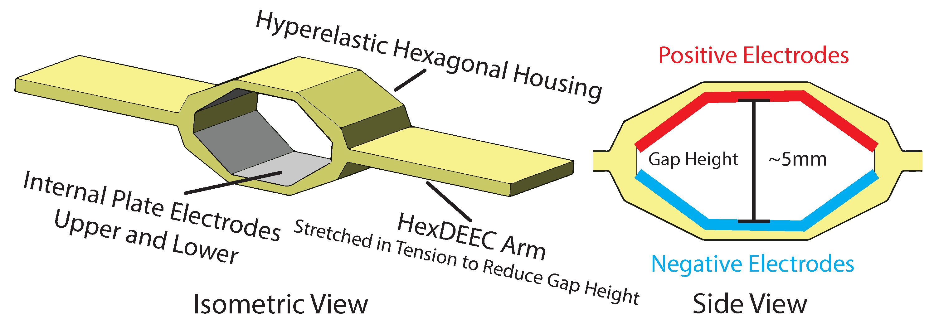
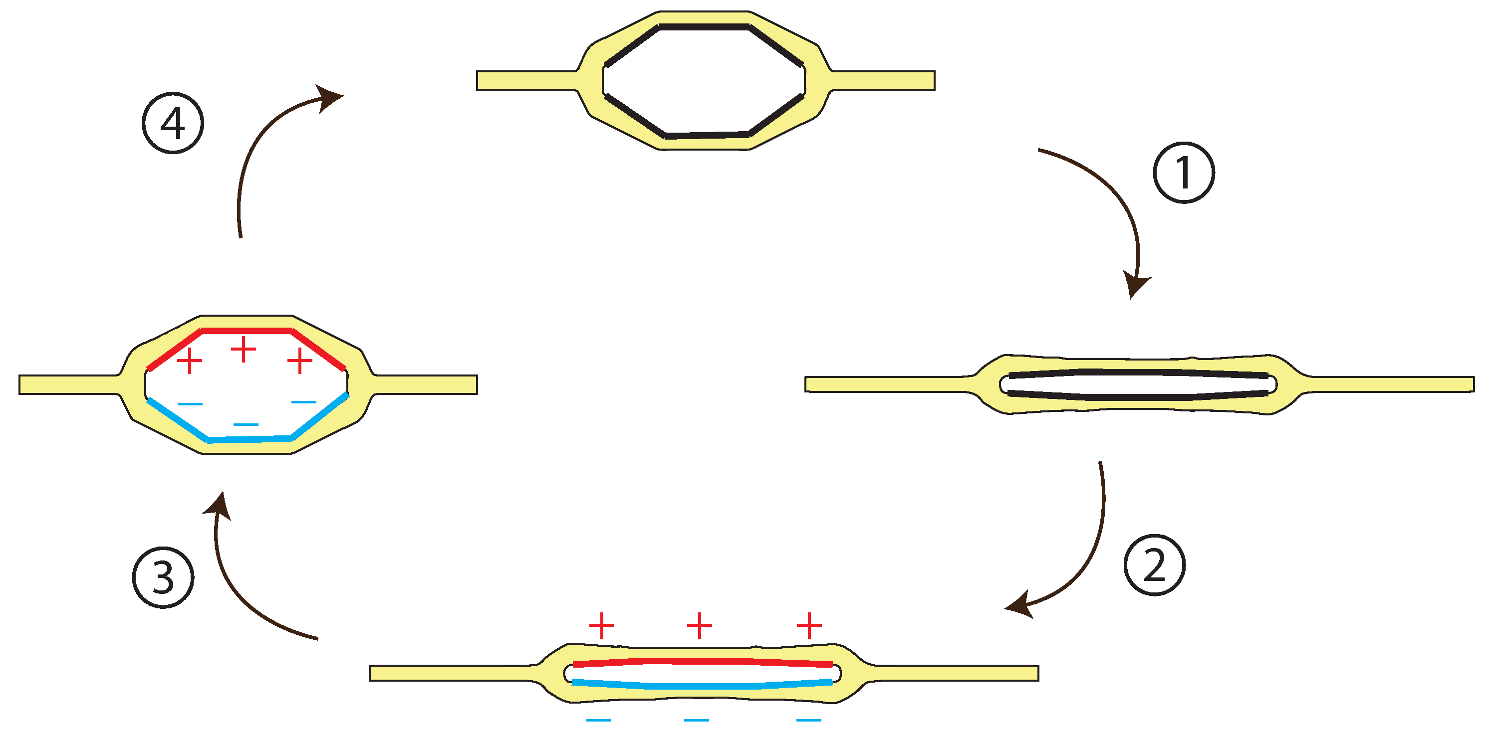
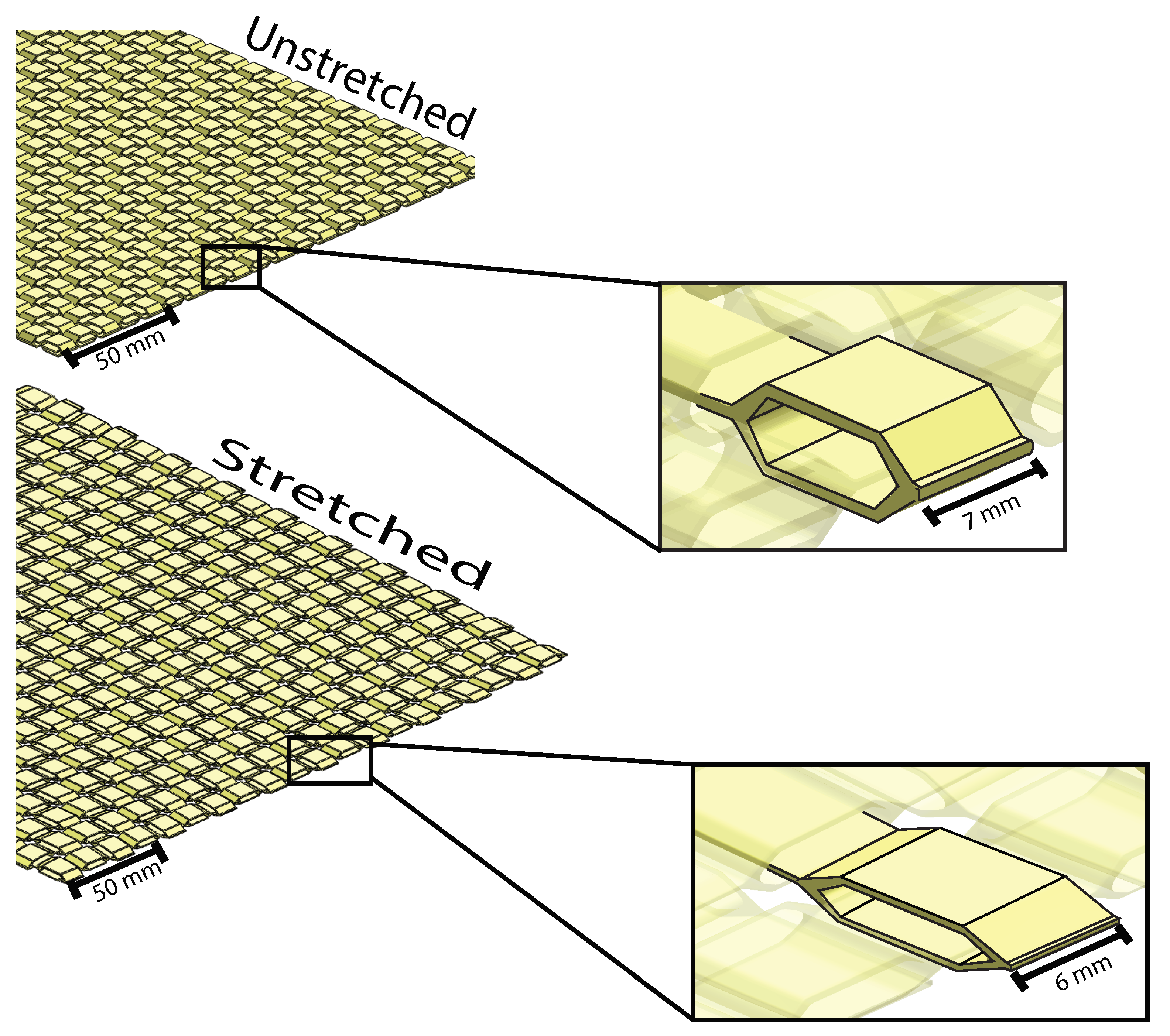
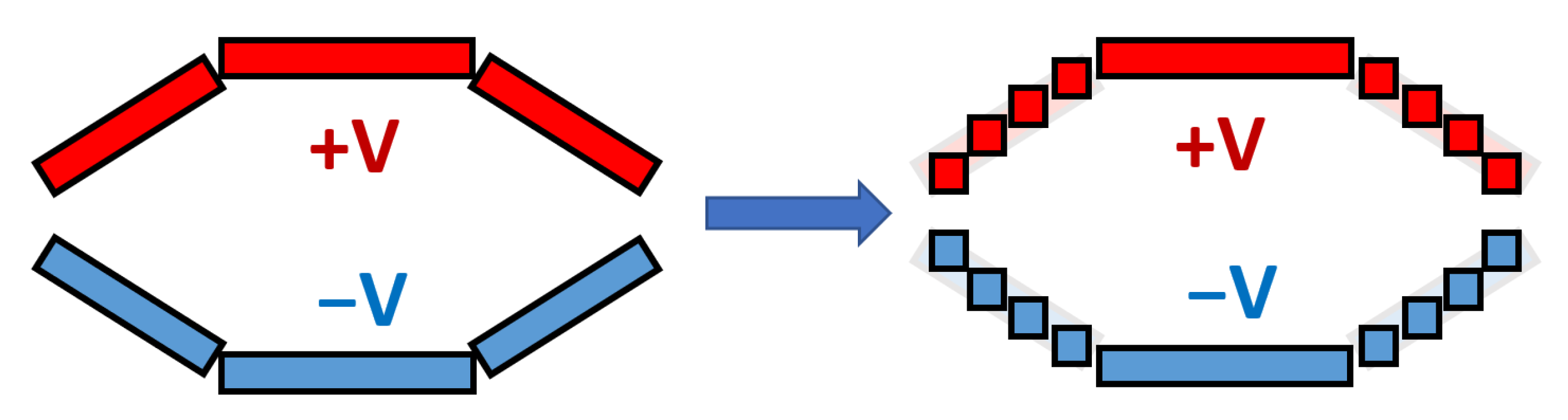
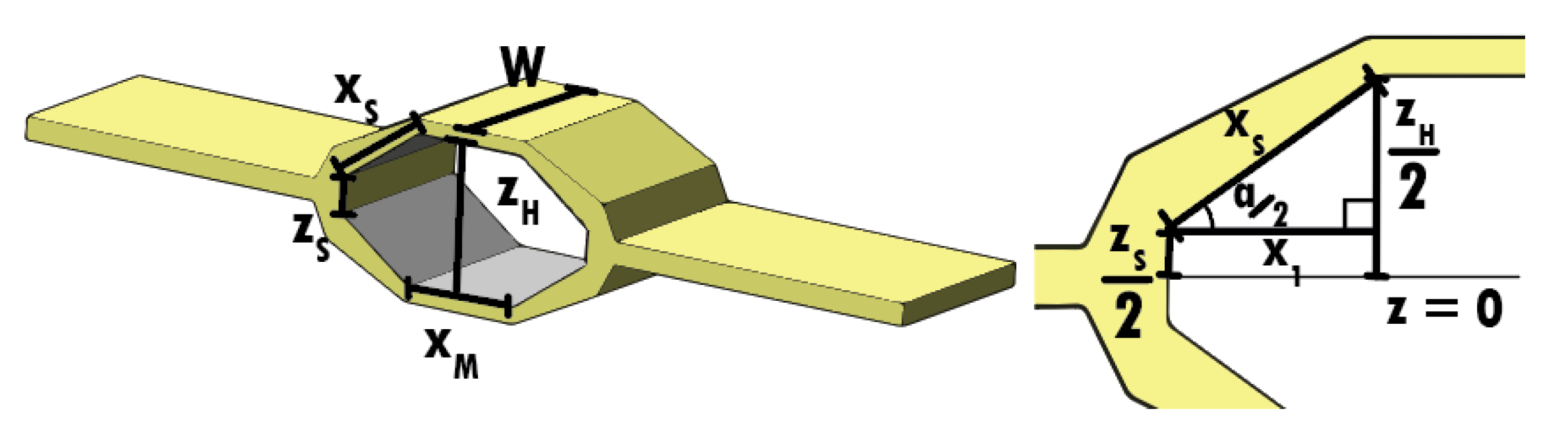
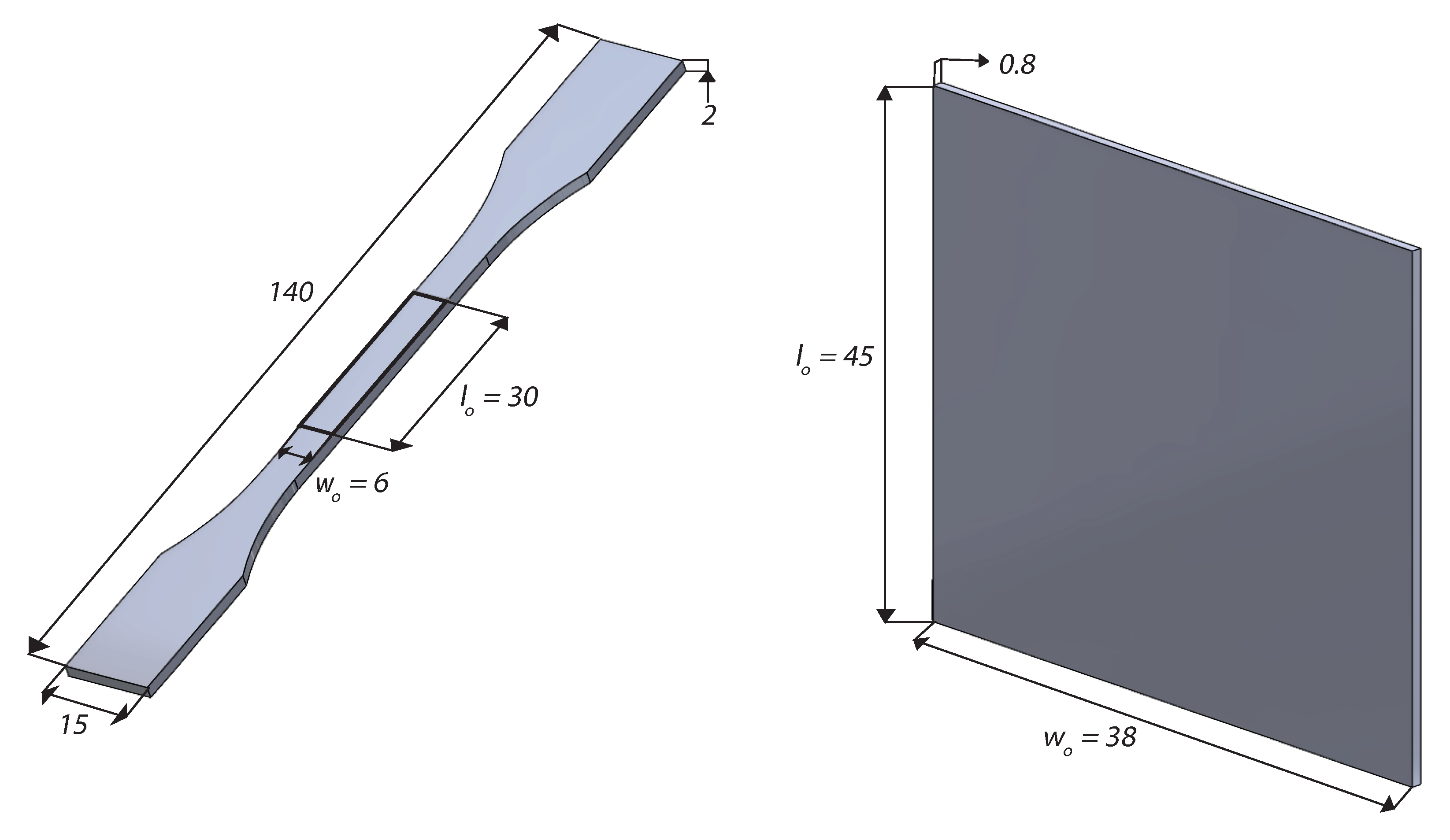
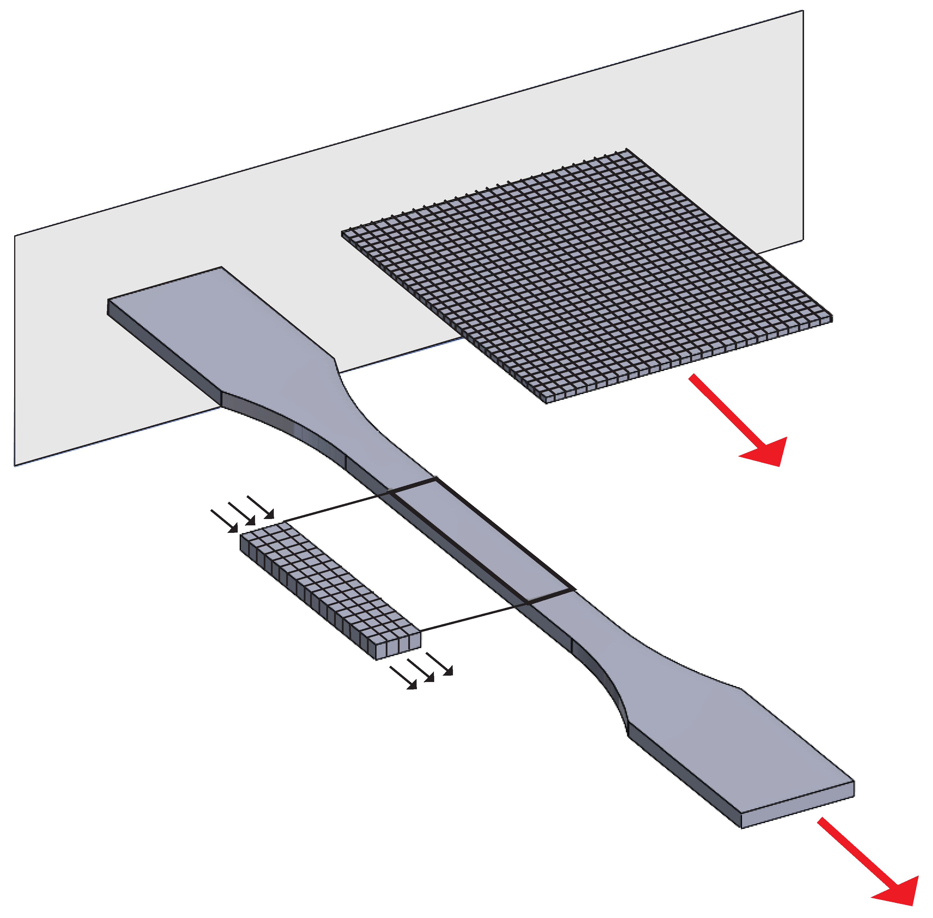
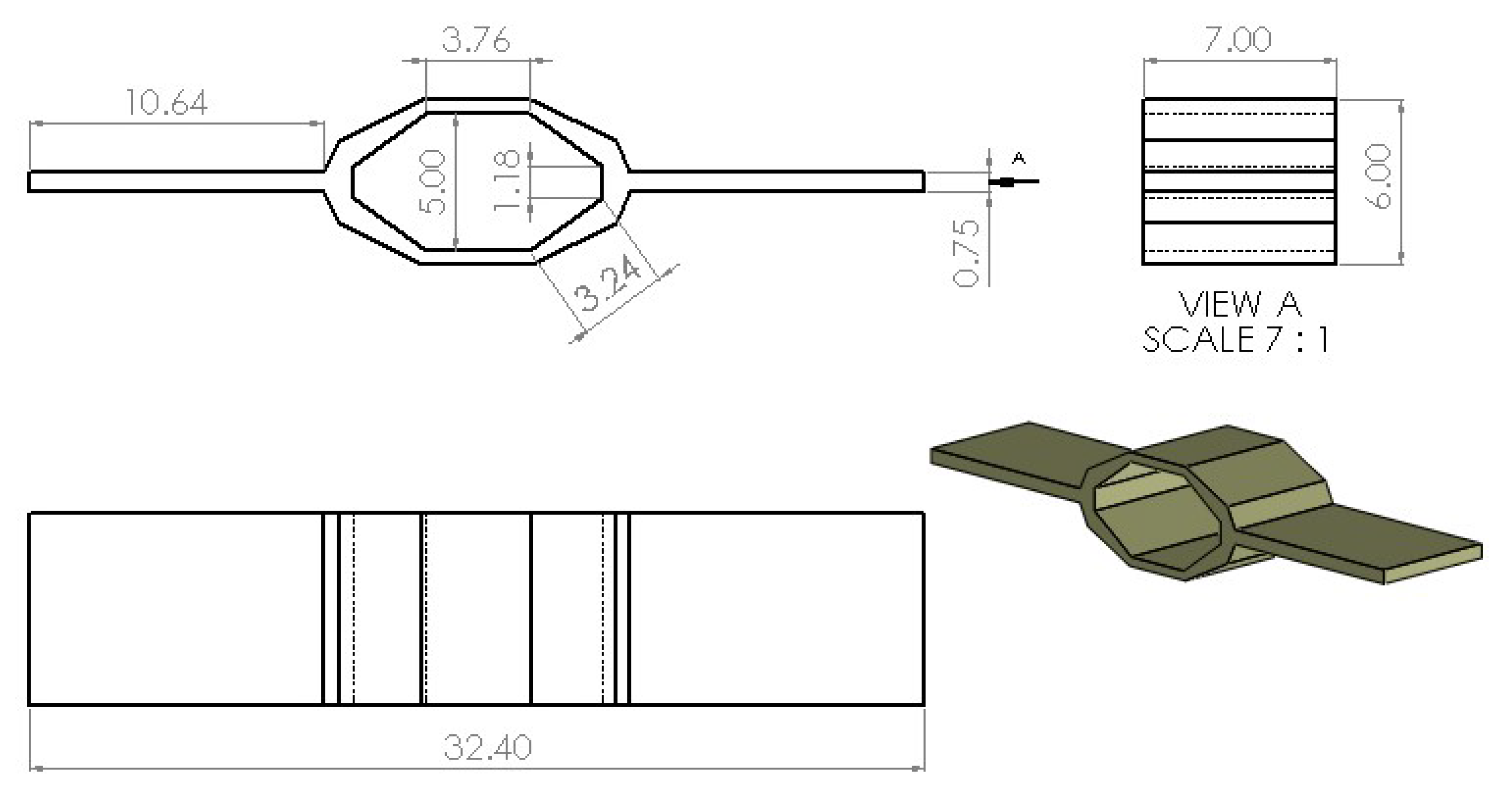
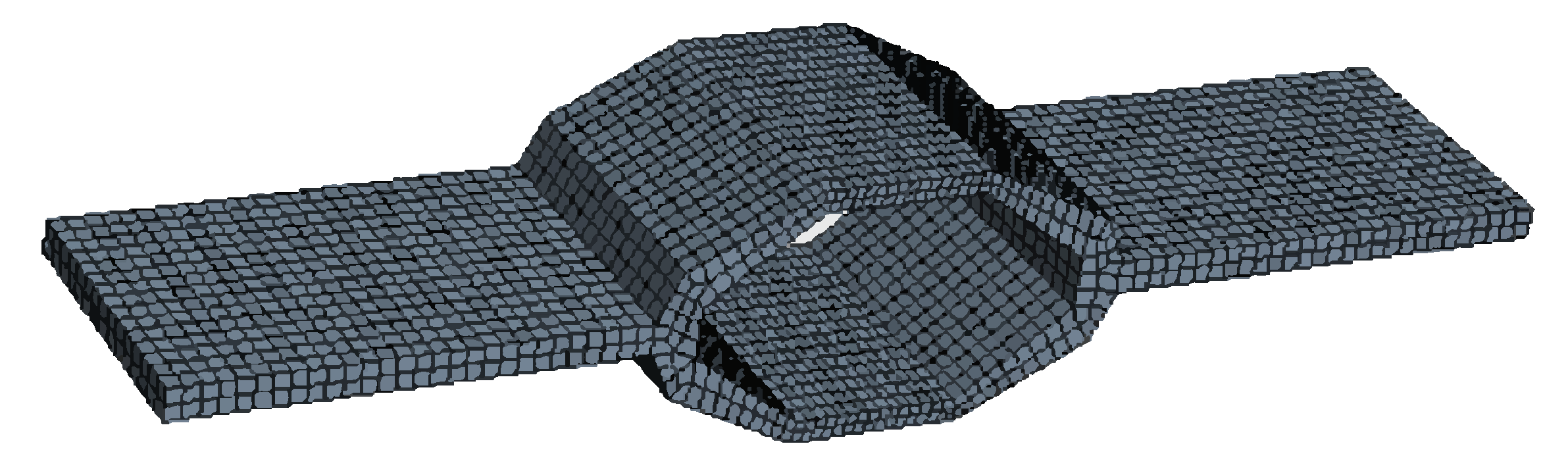
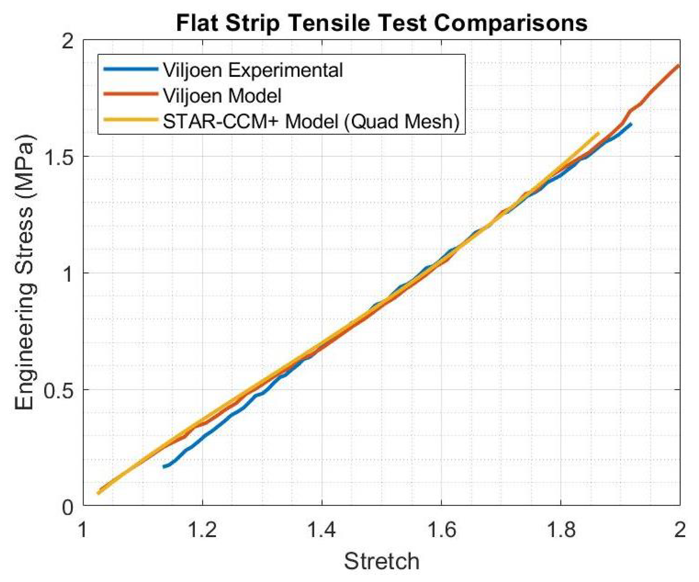
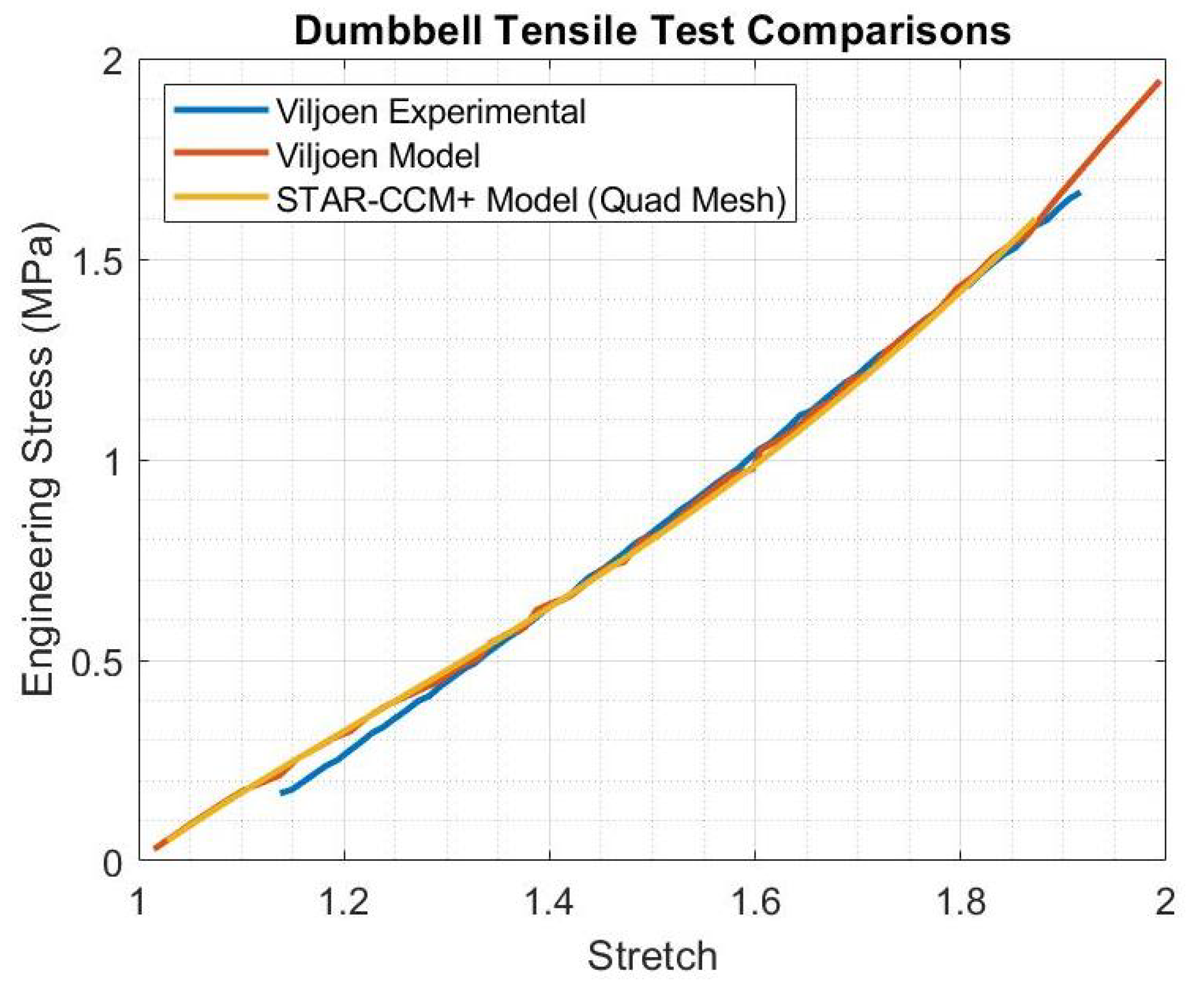
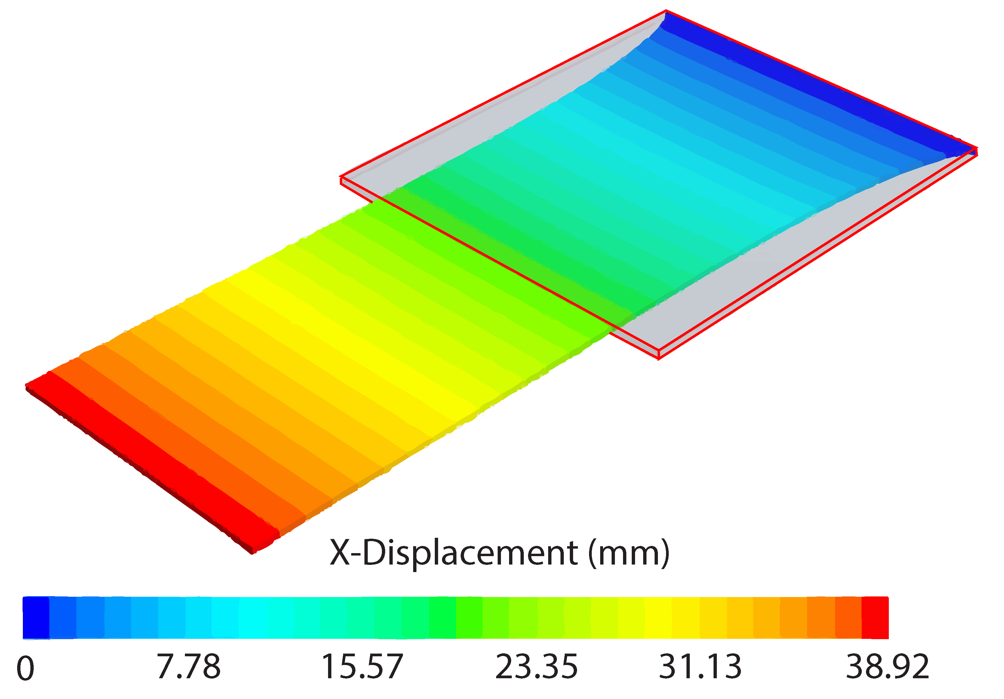
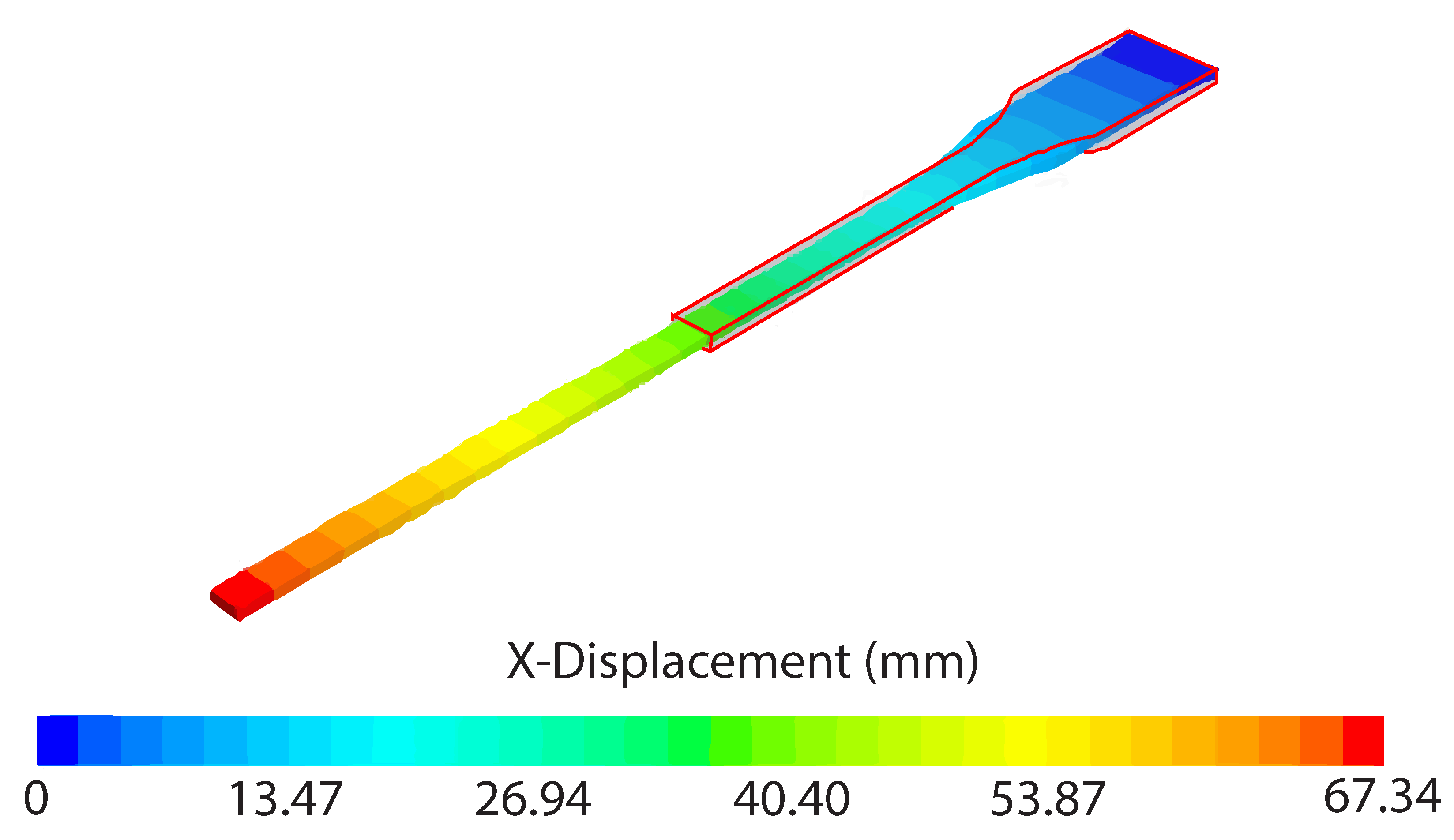
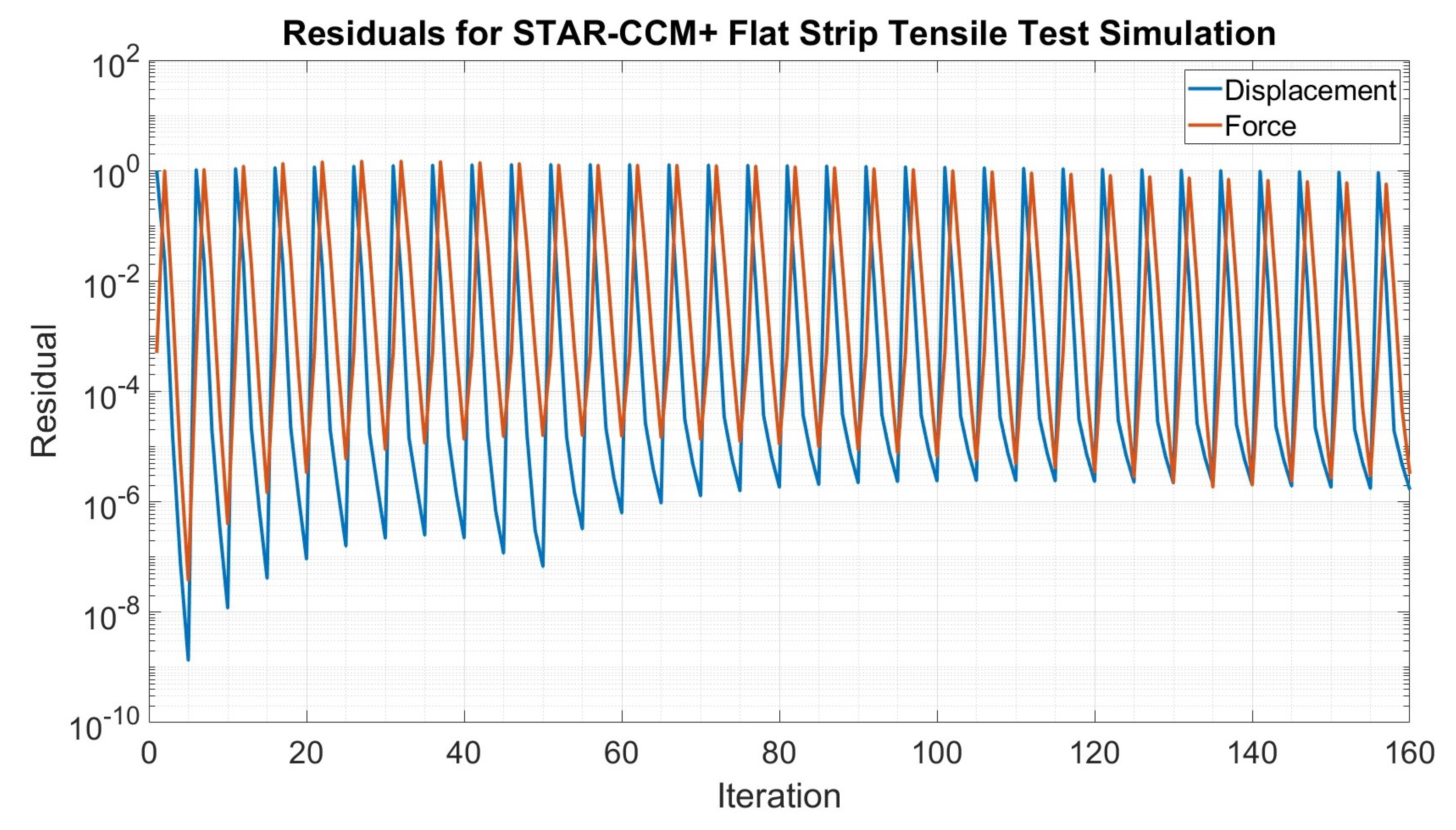
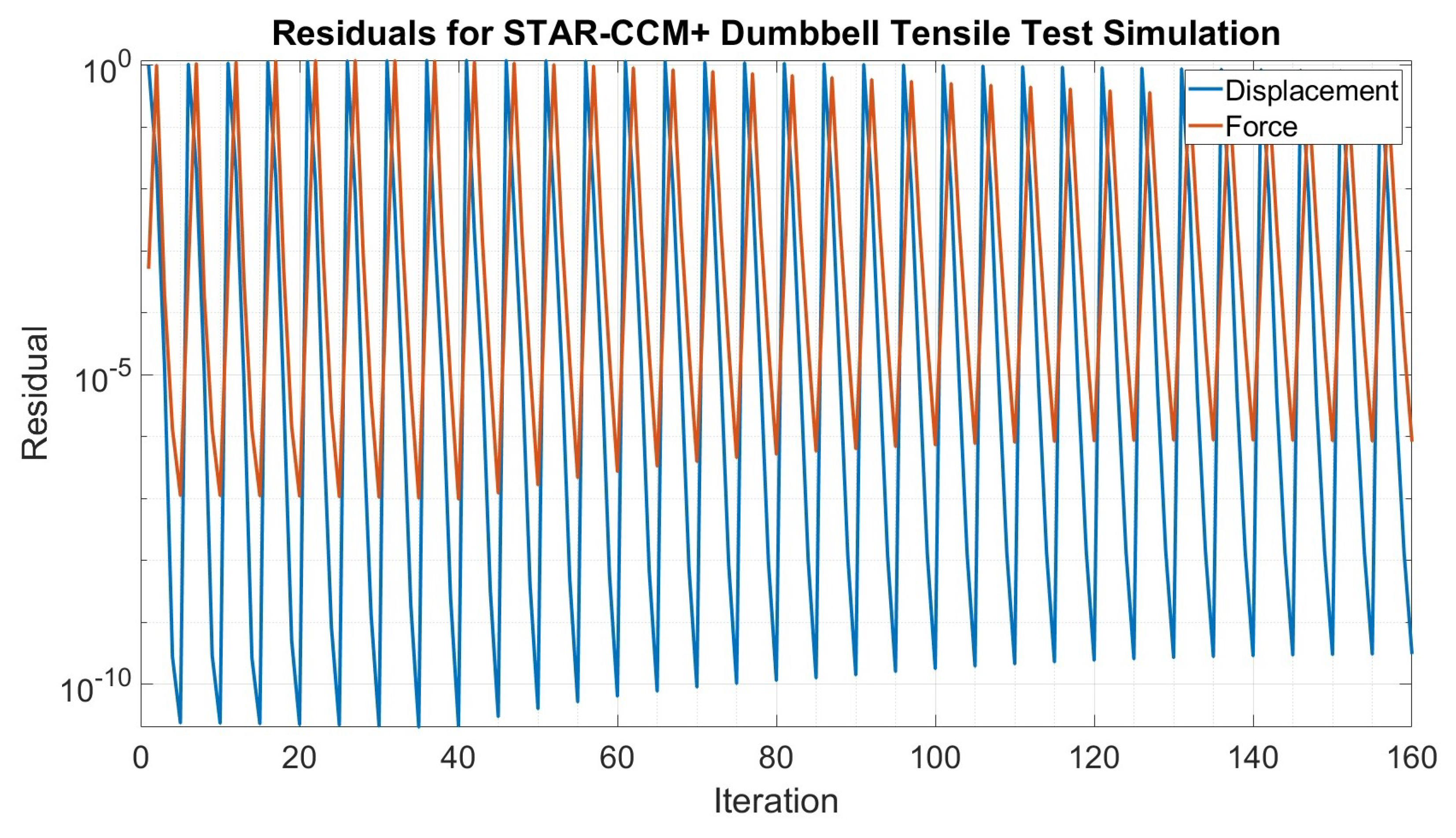
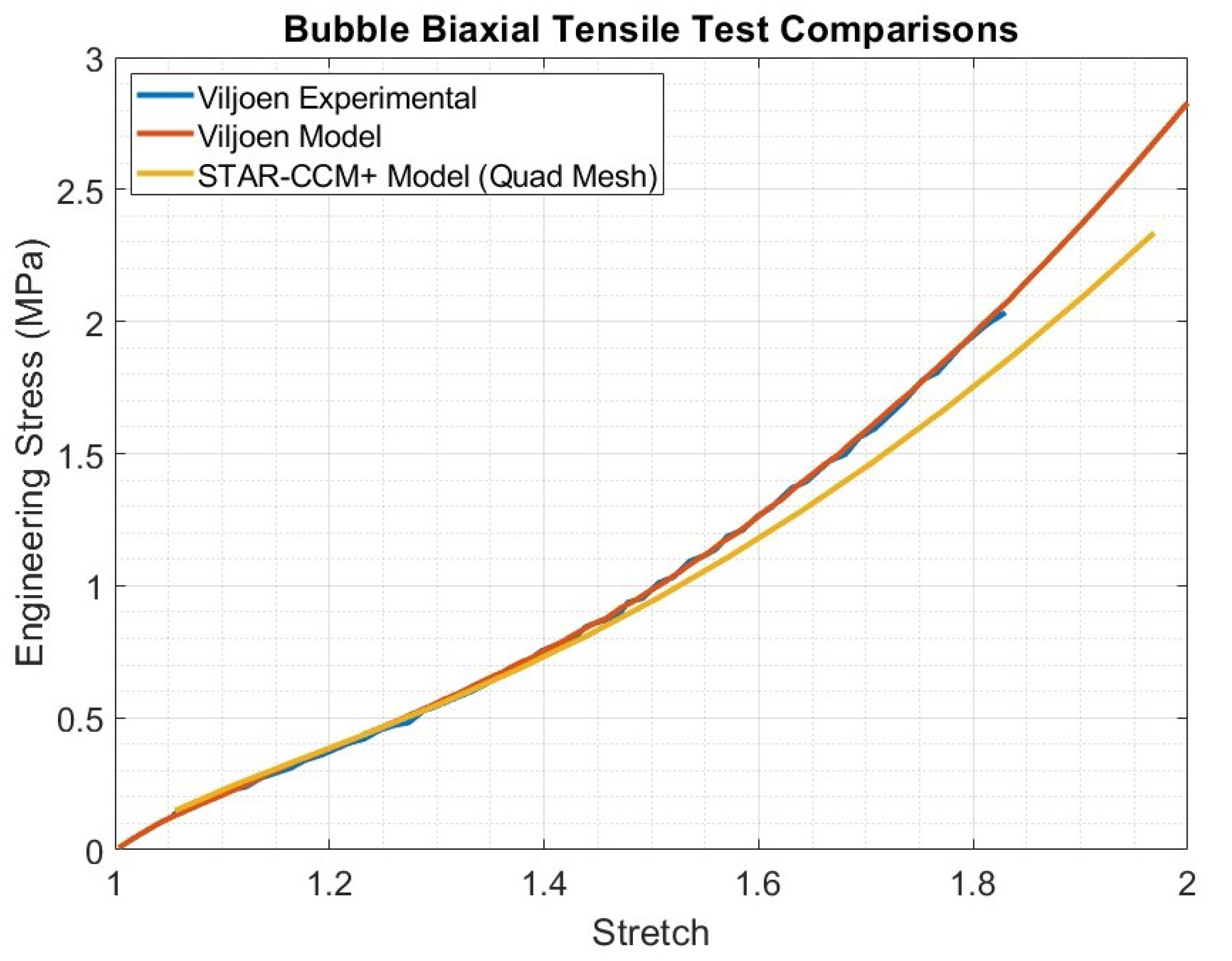
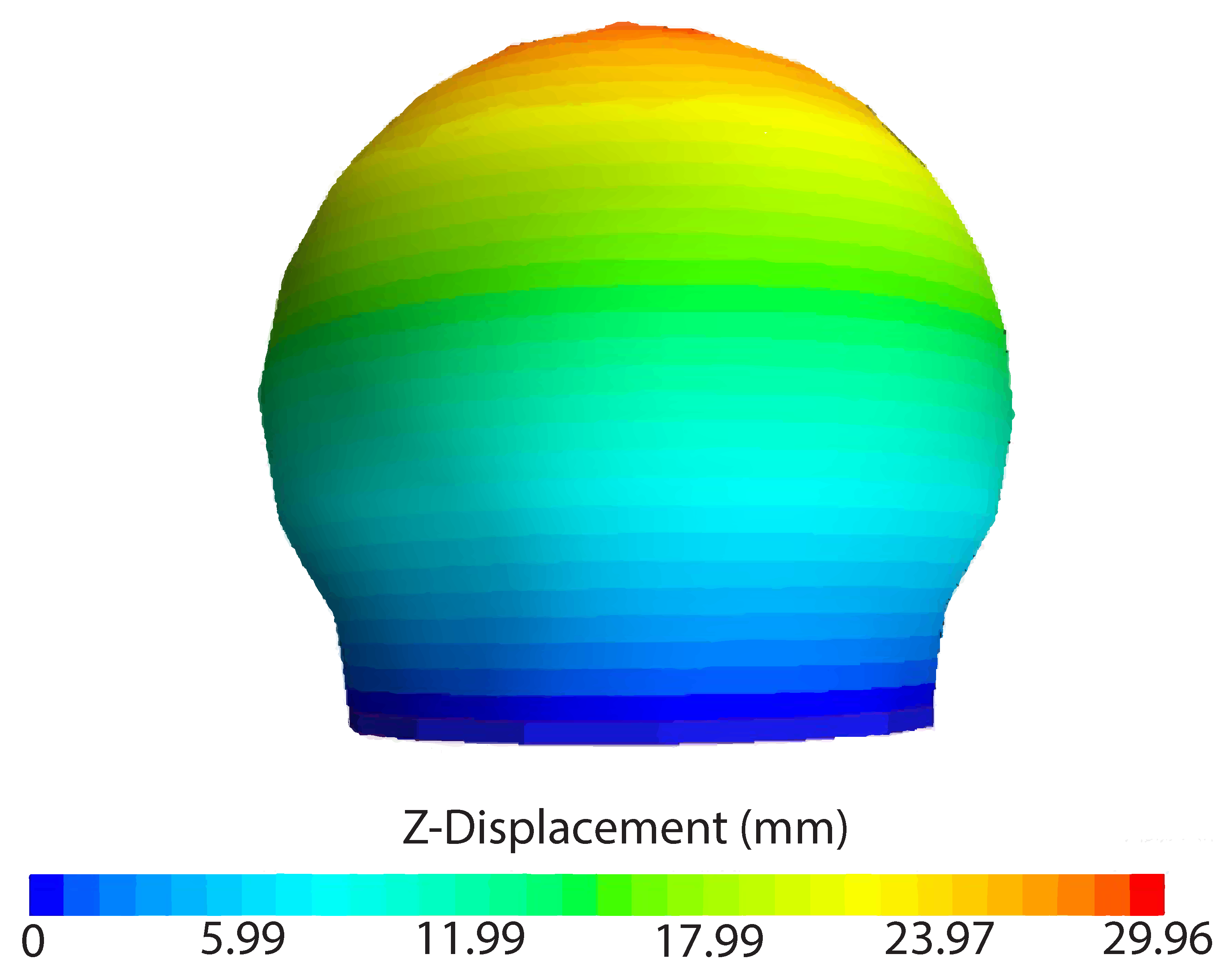
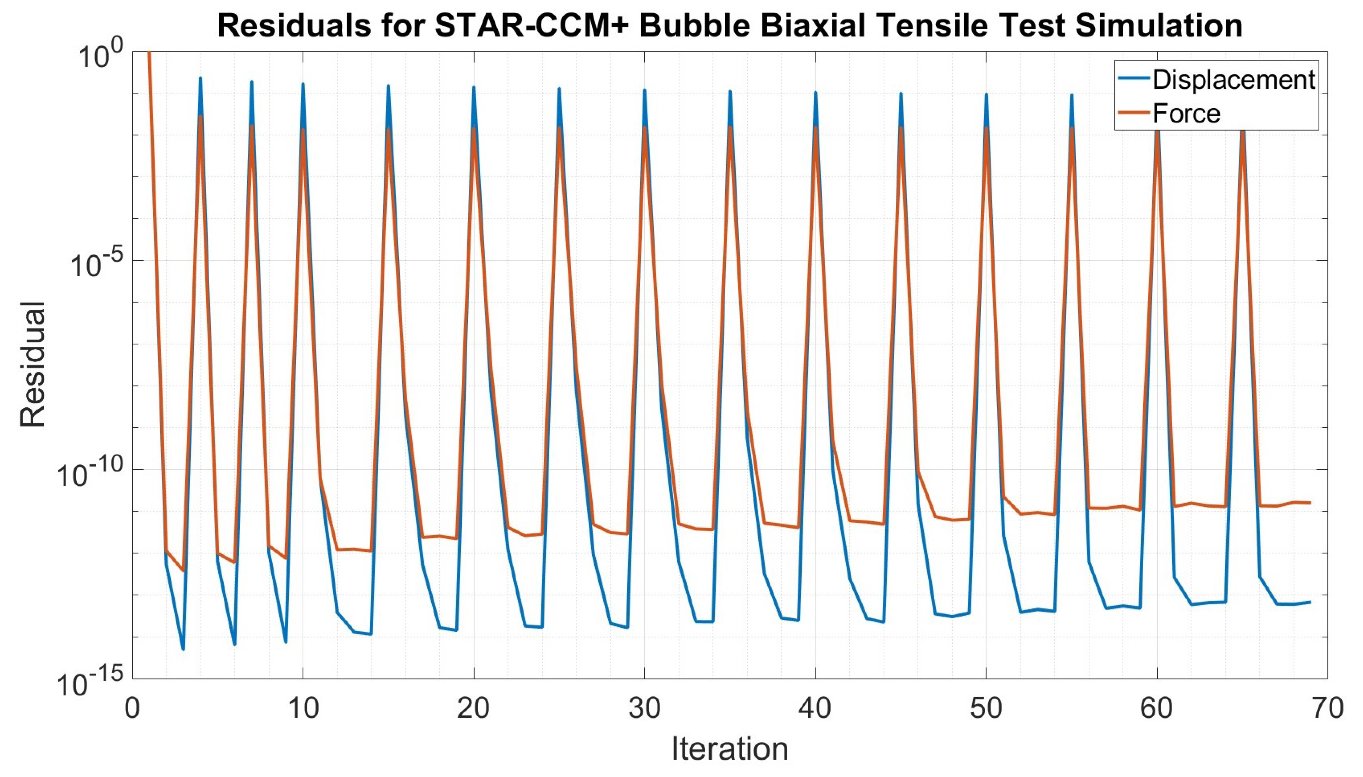
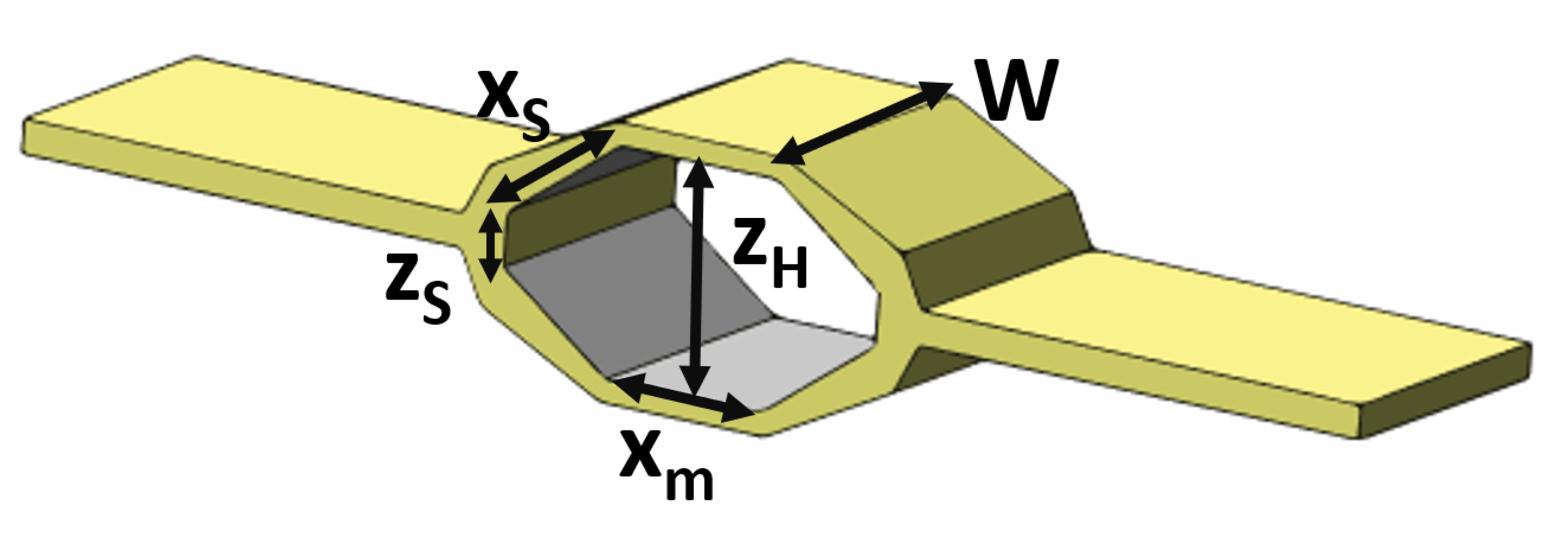
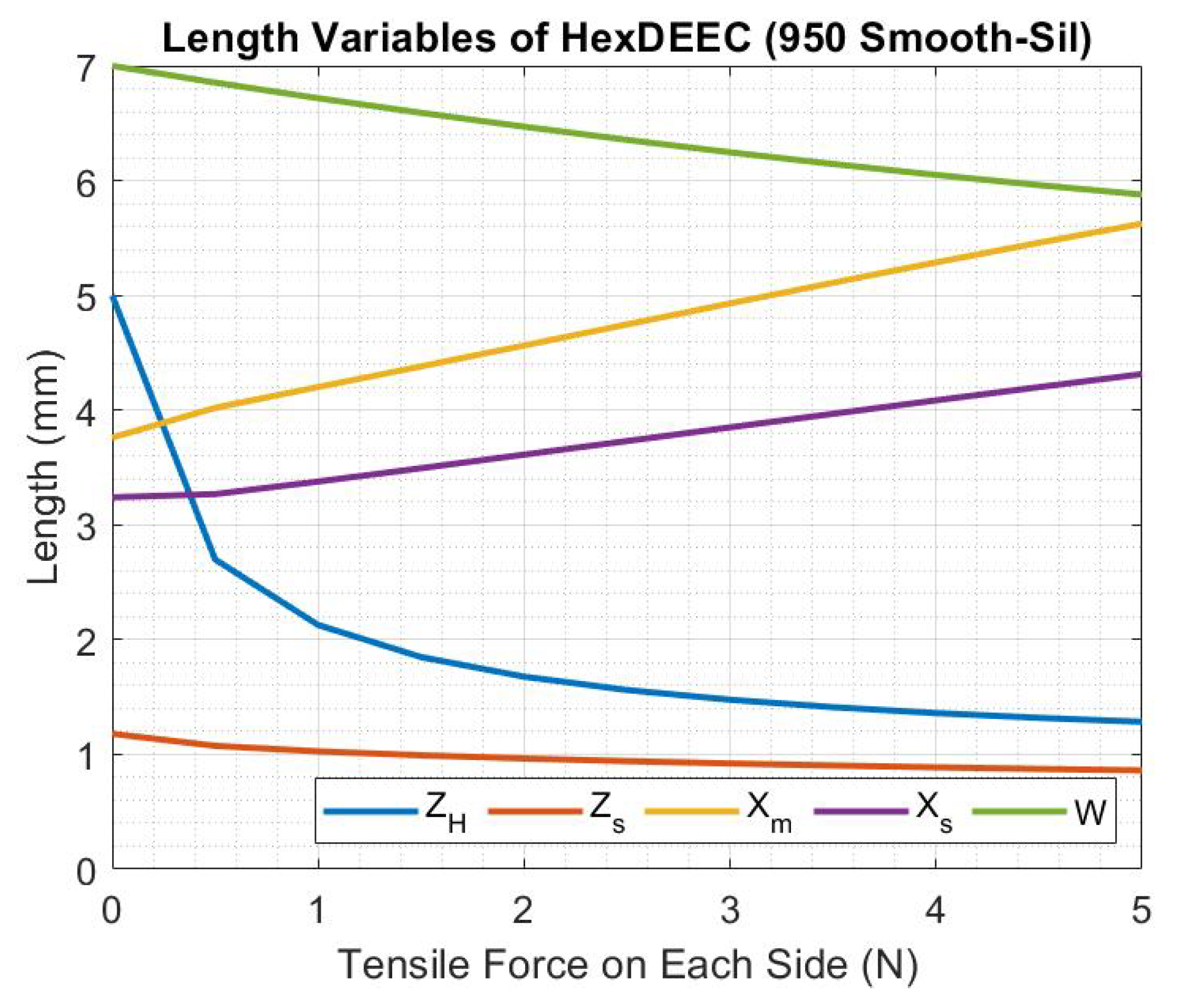
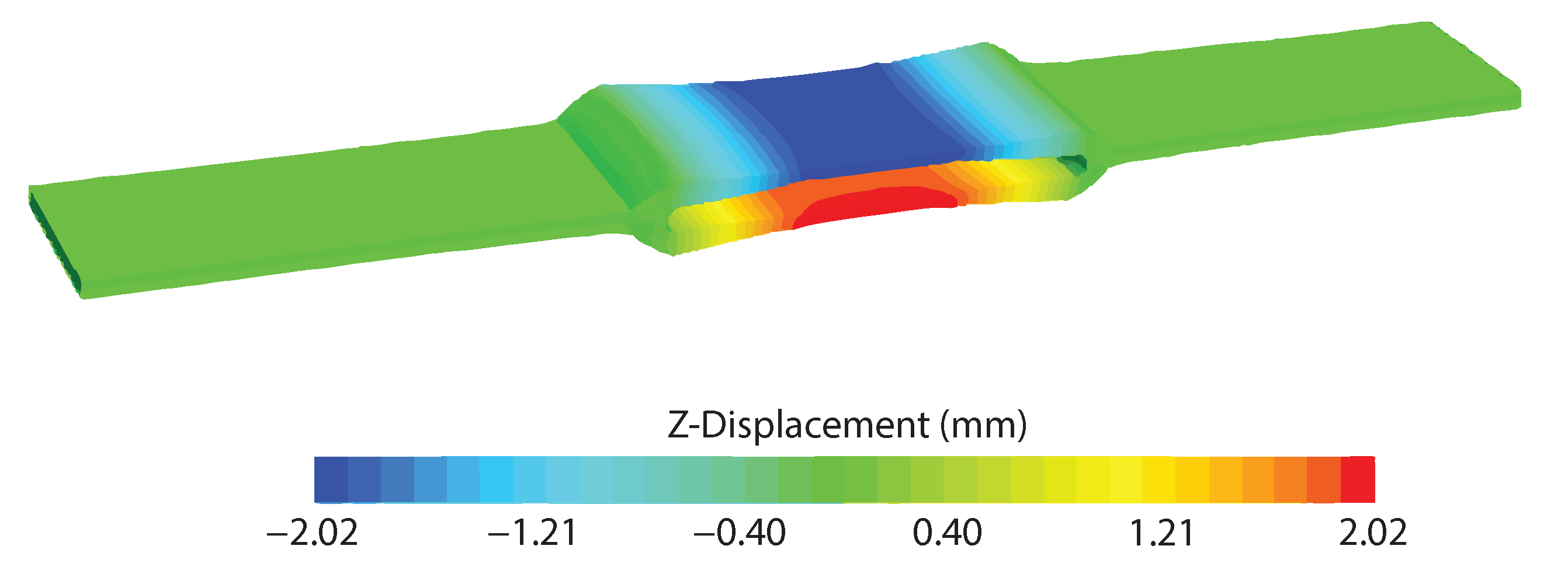
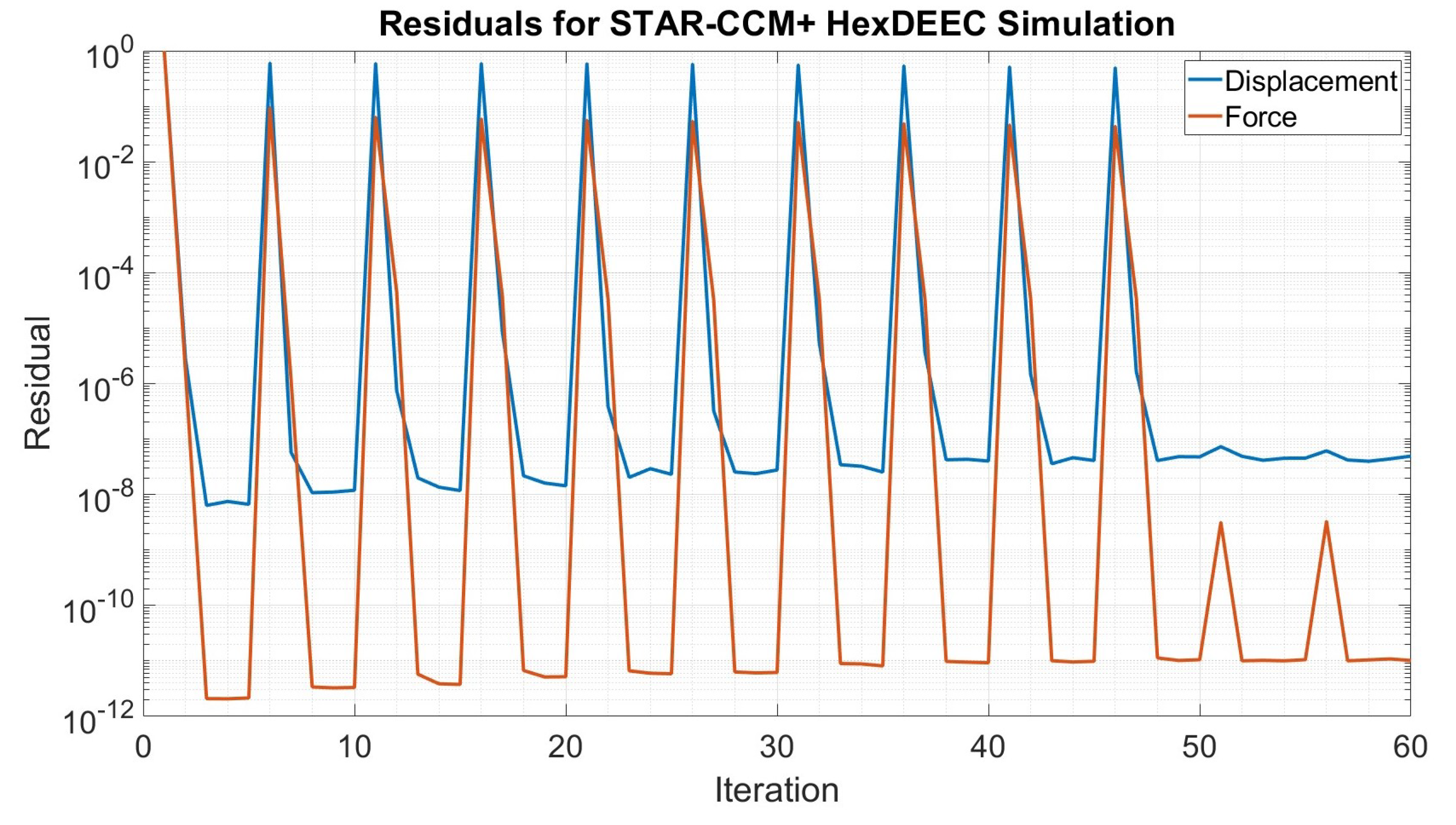
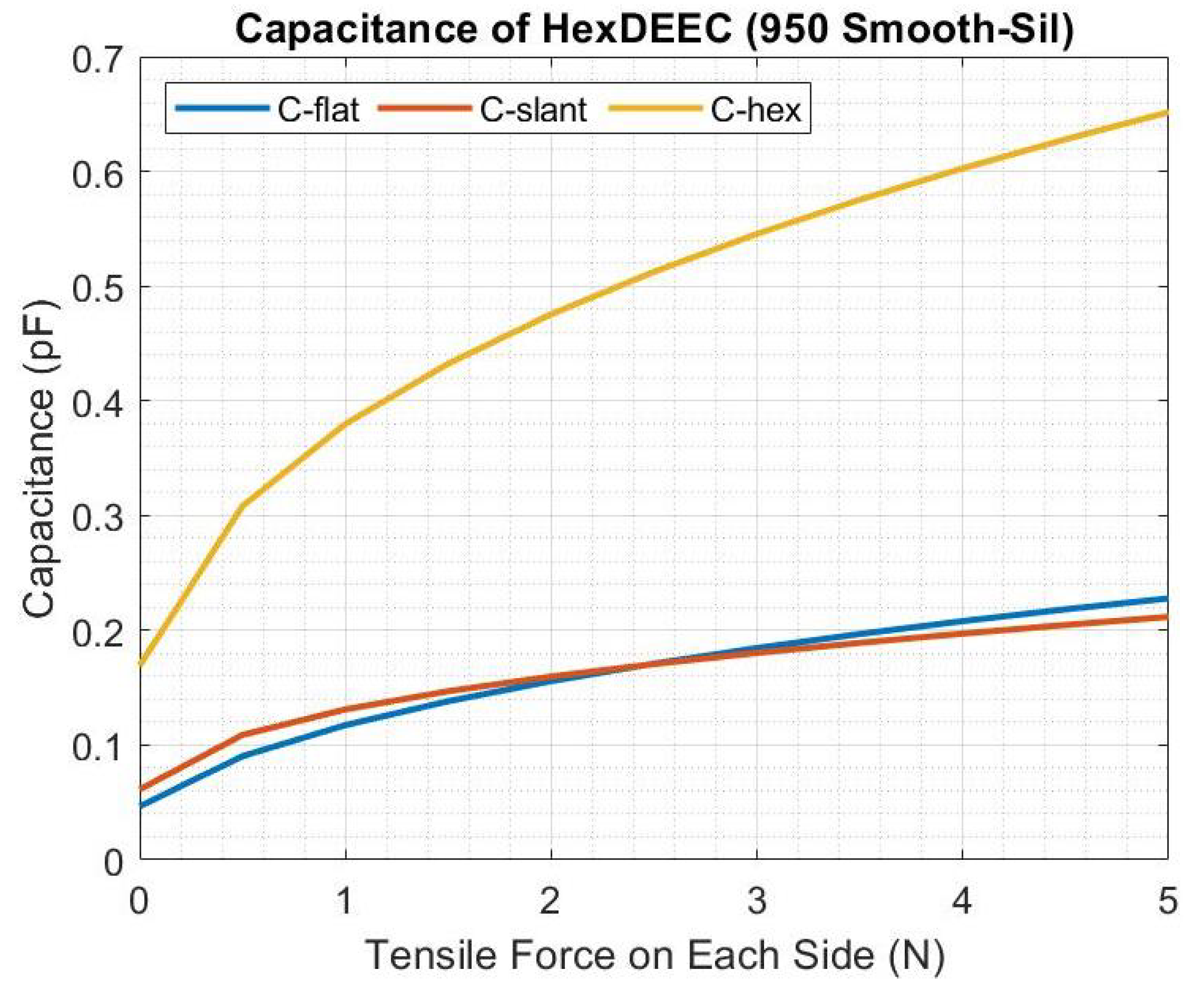
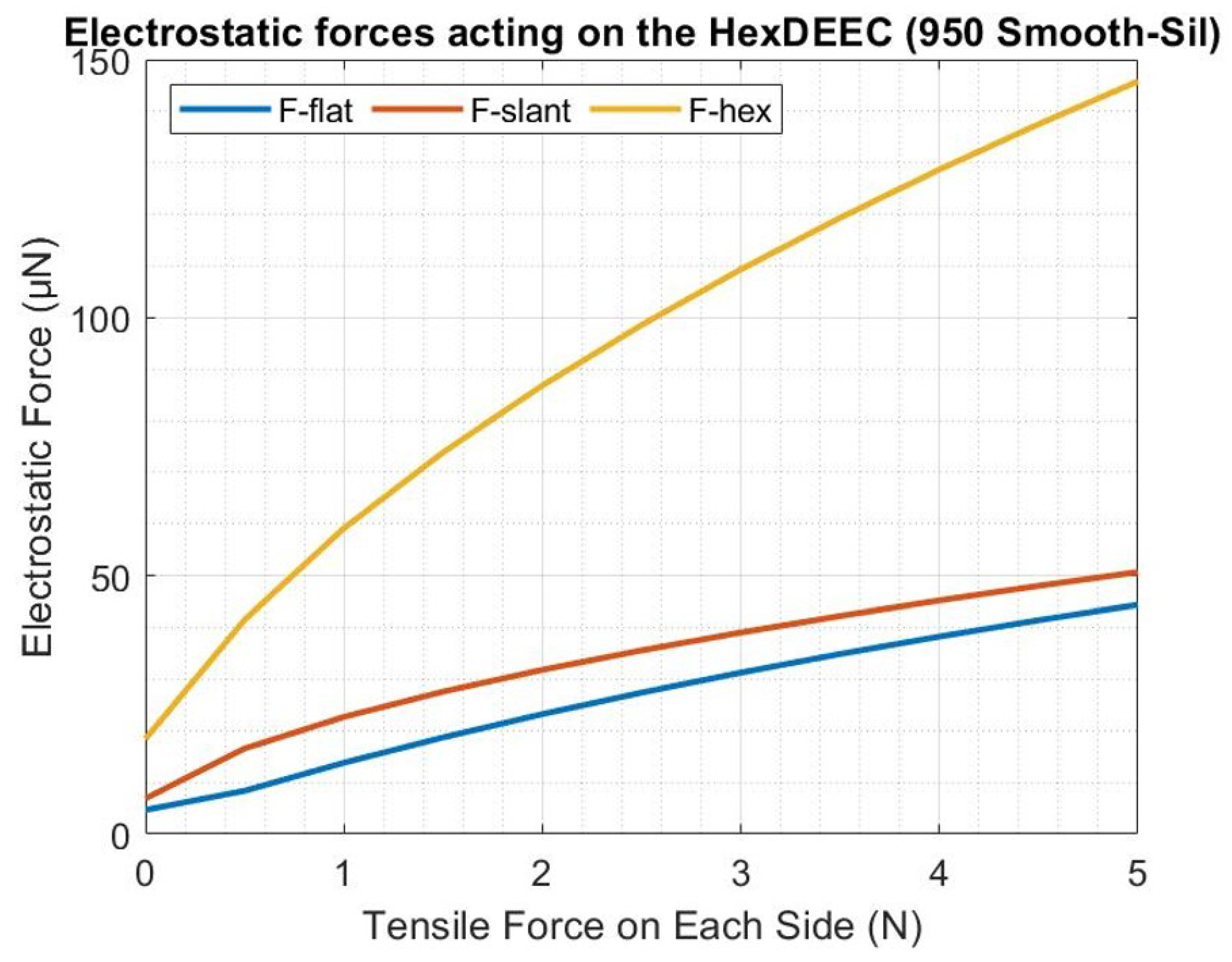
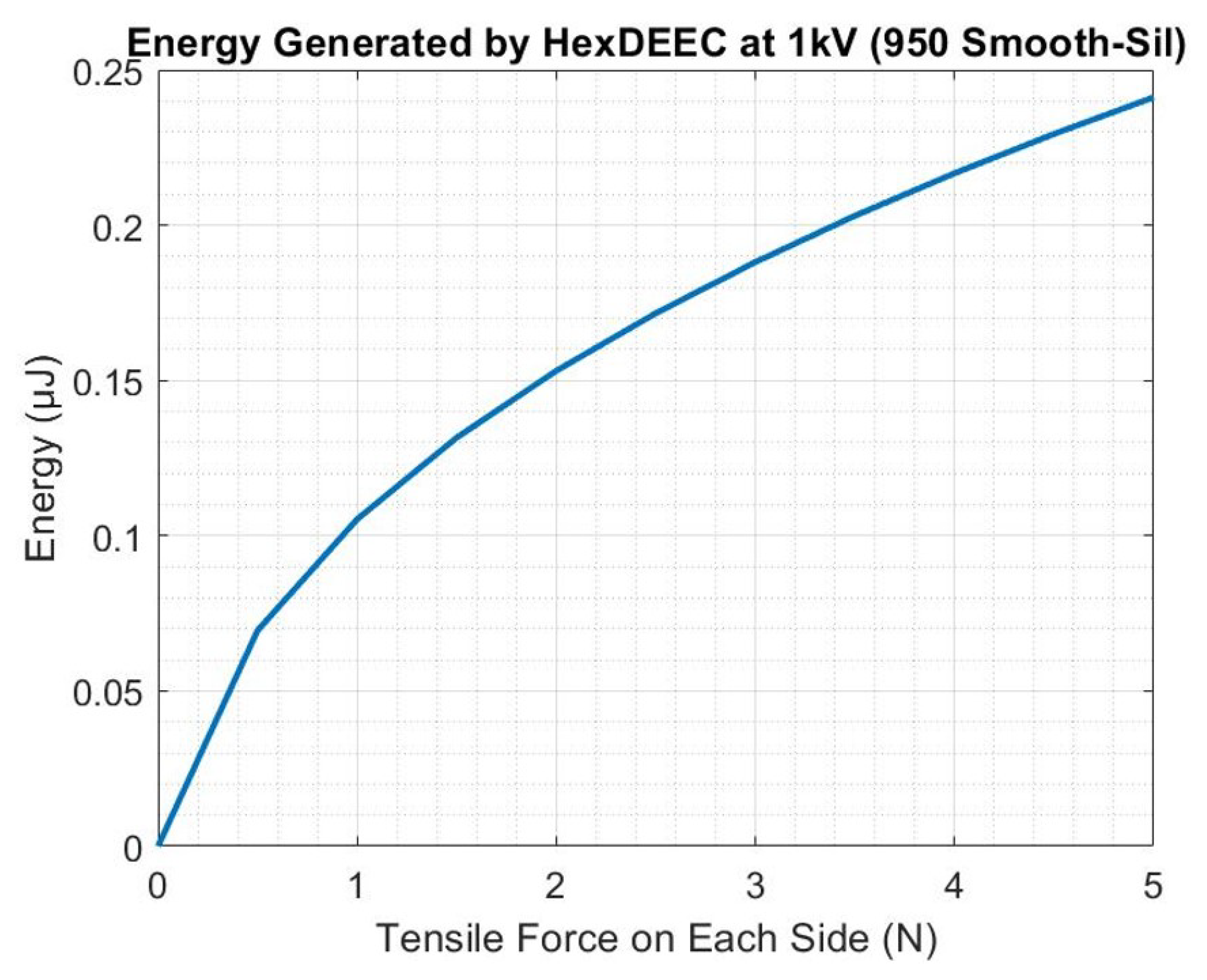
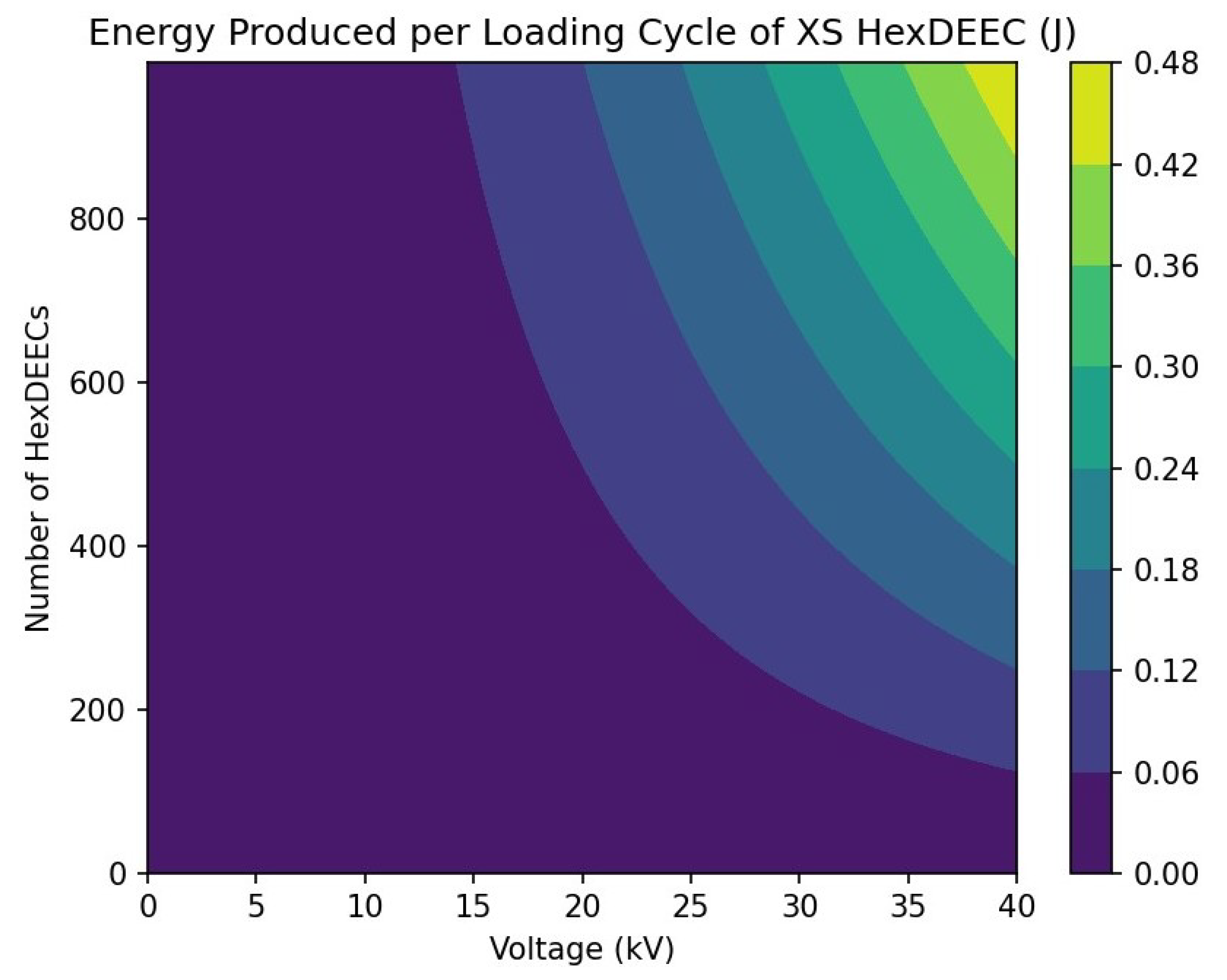
Table 1.
Hyperelastic material constants adapted from Viljoen and used for comparing uniaxial tensile tests [22].
Table 1.
Hyperelastic material constants adapted from Viljoen and used for comparing uniaxial tensile tests [22].
| Sample | (Pa) | (Pa) | (Pa) |
|---|---|---|---|
| Rectangular Flat Strip | 343,879.29 | 0.0 | 48,820.41 |
| Dumbbell Shaped | 306,269.50 | 0.0 | 62,791.08 |
Table 2.
Hyperelastic material constants adapted from Viljoen and used for comparing biaxial tensile inflation tests [22].
Table 2.
Hyperelastic material constants adapted from Viljoen and used for comparing biaxial tensile inflation tests [22].
| Sample | (Pa) | (Pa) | (Pa) |
|---|---|---|---|
| Bubble Membrane | 391,166.63 | −152,451.75 | 92,171.05 |
Disclaimer/Publisher’s Note: The statements, opinions and data contained in all publications are solely those of the individual author(s) and contributor(s) and not of MDPI and/or the editor(s). MDPI and/or the editor(s) disclaim responsibility for any injury to people or property resulting from any ideas, methods, instructions or products referred to in the content. |
© 2023 by the authors. Licensee MDPI, Basel, Switzerland. This article is an open access article distributed under the terms and conditions of the Creative Commons Attribution (CC BY) license (https://creativecommons.org/licenses/by/4.0/).
Share and Cite
MDPI and ACS Style
Niffenegger, J.S.; Boren, B. Numerical Methods to Evaluate Hyperelastic Transducers: Hexagonal Distributed Embedded Energy Converters. Energies 2023, 16, 8100. https://doi.org/10.3390/en16248100
AMA Style
Niffenegger JS, Boren B. Numerical Methods to Evaluate Hyperelastic Transducers: Hexagonal Distributed Embedded Energy Converters. Energies. 2023; 16(24):8100. https://doi.org/10.3390/en16248100
Chicago/Turabian StyleNiffenegger, James Salvador, and Blake Boren. 2023. "Numerical Methods to Evaluate Hyperelastic Transducers: Hexagonal Distributed Embedded Energy Converters" Energies 16, no. 24: 8100. https://doi.org/10.3390/en16248100
Note that from the first issue of 2016, this journal uses article numbers instead of page numbers. See further details here.