
Power Distribution Systems’ Vulnerability by Regions Caused by Electrical Discharges

1
Department of Electrical Engineering, São Paulo State University (UNESP), Ilha Solteira 15385-000, São Paulo, Brazil
2
Department of Energy Engineering, São Paulo State University (UNESP), Rosana 19274-000, São Paulo, Brazil
*
Author to whom correspondence should be addressed.
Energies 2023, 16(23), 7790; https://doi.org/10.3390/en16237790
Submission received: 19 October 2023
/
Revised: 20 November 2023
/
Accepted: 23 November 2023
/
Published: 27 November 2023
(This article belongs to the Section F: Electrical Engineering)
Abstract
:Energy supply interruptions or blackouts caused by faults in power distribution feeders entail several damages to power utilities and consumer units: financial losses, damage to power distribution reliability, power quality deterioration, etc. Most studies in the specialized literature concerning faults in power distribution systems present methodologies for detecting, classifying, and locating faults after their occurrence. In contrast, the main aim of this study is to prevent faults by estimating the city regions whose power grid is most vulnerable to them. In this sense, this work incorporates a geographical-space study via a spatial data analysis using the local variable electrical discharge density that can increase fault risks. A geographically weighted spatial analysis is applied to data aggregated by regions to produce thematic maps with the city regions whose feeders are more vulnerable to failures. The spatial data analysis is implemented in QGIS and R programming environments. It is applied to the real data of faults in distribution power grid transformers and electrical discharges in a medium-sized city with approximately 200,000 inhabitants. In this study, we highlight a moderate positive correlation between electrical discharge density and the percentage of faults in transformers by regions in the central and western areas of the city under study.
1. Introduction
Energy supply interruptions (ESIs) or faults are events associated with the operational process of power distribution systems (PDSs) [1]. They are classified into two categories: temporary and permanent. Transient faults occur in a very short time (in the order of milliseconds). After this, a PDS is automatically restored. On the other hand, there is no electrical system restoration in the occurrence of a permanent fault. In this case, the PDS returns to its nominal operating conditions after the fault location and removal [2].
An ESI causes substantial financial losses for power utilities and consumer units (CU) that share the same distribution power grid. In this sense, electrical discharges represent a relevant cause of an ESI; furthermore, they are associated with damage to electrical equipment [3]. With the energy market’s development, an energy supply with good quality and reliability become a relevant factor for power grid operators [4]. Thus, an ESI depreciates the PDS indices of quality and reliability [5], where fault events represent 80% to 90% of the times without energy supply to CUs [6].
In this context, there are several factors associated with ESIs: (i) adverse weather conditions, (ii) fires, (iii) tree vegetation close to the overhead power distribution, (iv) human failures, and (v) equipment failures (due to manufacturing defect, lack of maintenance, or obsolescence) [2,7].
The National Electrical System Operator (ONS) presented a statistical report of the main factors responsible for faults in Brazilian power grids, as shown in Table 1. Adverse weather conditions such as electrical discharges, heavy rains, storms, and wind gusts are the main ESI causes, with approximately 30% participation [7].
Additionally, Table 1 shows the reasons associated with ESI, representing an average among Brazilian cities. In this sense, consider a town on the northeast coast of Brazil, where wind gusts are the main reason for faults in distribution feeders. Meanwhile, they are not associated with ESIs for another city in the central region with different weather conditions such as those of coastal towns. Therefore, various factors cause ESIs in other areas. Thus, incorporating spatial data analysis (SDA) helps understand which factors are relevant to a city region becoming more vulnerable to ESIs.
To the best of the authors’ knowledge, most studies in the specialized literature prioritize fault detection and location after their occurrence. For example, in [8,9,10,11,12], fault detection and classification were performed considering various fault scenarios. On the other hand, estimating regions in which the power grid distribution is more vulnerable to failures provides crucial information for planning measures to avoid inconveniences and additional costs arising after steady-state faults occur.
Reducing the time of ESIs is essential for improving the power quality in a PDS [13]. In this context, estimating regions vulnerable to failures assists in decision-making and identifying critical areas that must be prioritized for replacing damaged equipment. Thus, power supply with more excellent quality and reliability is ensured.
In this sense, this study aims to incorporate the analysis of geographic space for estimating city regions whose utility grid is more vulnerable to failures. It is assumed that some local factors or variables interfere with the utility grid, making it more vulnerable to failures. These local factors or variables are shown in Table 1: adverse weather conditions such as electrical discharges, tree vegetation, and fires.
In this context, geographic information systems (GISs) are essential to an SDA for estimating regions vulnerable to faults. They are used in managing, planning, and controlling power grids. They comprise geoprocessing tools for collecting, storing, analyzing, and displaying geographic data. A GIS application enables power grid visualization, which is affected by local factors that belong to the region where it is located, as well as other power utility assets, such as substations, transformers, and protection equipment [14,15].
According to [16], the first step in an SDA is to perform an exploratory analysis of spatial or georeferenced data. An exploratory analysis consists of the graphical representation of data available on thematic maps or heat maps and the incorporation of descriptive statistics metrics considering the geographic space.
Thus, this study performs a geographically weighted exploratory analysis (GWEA) on geographic data from a Brazilian city. Crucial for this study are the georeferenced data and the weighting matrix. In the former, georeferenced data are those whose geographical coordinates of the phenomenon under investigation are known. In the latter, the weighting matrix represents the urban zone’s neighborhood structure because it allows for characterizing the influence among small regions or census tracts (CTs).
Therefore, the first step of an SDA with aggregated data in small regions or CTs is performed in this study: GWEA. It is performed based on a local factor or variable frequently associated with faults in a PDS: electrical discharges. It is determined whether these local variables become the utility grid in some city regions more vulnerable to failures. Therefore, GWEA is applied to data aggregated by small areas or CTs to produce thematic maps with the city regions whose feeders are more susceptible to failures.
1.1. Literature Review
A fault incidence matrix method was introduced in [4] to evaluate the reliability of a medium voltage distribution grid. The authors presented a reliability calculation unit called M-Segment-N-tie-switch (MSNT), which included several distribution grid structures; thus, the method became applicable for different systems’ operating conditions. Each MSNT was associated with a matrix of a power supply path obtained by inversing the node branch incidence matrix. Subsequently, it was used to obtain the fault incidence matrix. The reliability indices for each system load were calculated, where the fault incidence matrix and the vectors of fault events’ characteristics were applied. The technique improved the reliability efficiency, as it avoided some procedures such as the fault events enumeration and the repetitive search for the fault influence range. Furthermore, the technique is intuitive and enables a sensitivity analysis and system vulnerability identification.
In [17], a GIS-based tool for spatial analysis in a PDS was presented. The authors applied spatial analysis techniques such as inverse distance weighting, slope, and contour maps. The load flow results were the input data for the ArcGIS, where several maps were produced to analyze the dynamic behavior of the PDS. The results showed that any disturbances occurring in the PDS were detected and controlled in real-time through the GIS application.
Chen and Kezunovic [18] proposed a fuzzy logic-based tool for the predictive analysis of ESIs. The authors highlighted the extreme climate impacts and their risk to the electrical system’s operation. Fuzzy logic was introduced to process weather information. Wind speeds and gusts were input parameters, whereas the fuzzy inference system provides an alert level as the output. A risk map was produced from the vulnerability results and processed using GIS. The risk results were shown as power-cut probability maps. Weather forecasts and operational data belonging to the system improved the decision-making process.
In [5], a data mining-based tool was proposed to determine fault probabilities. The technique was based on the Naive Bayes model, incorporating weather information, assets, and outage history. Feeder sections were classified according to their fault probability using GIS.
Zhou et al. [1] presented a methodology for assessing and managing fault risks in PDSs with distributed generation units. An island partitioning strategy was proposed to improve accuracy and speed in the evaluation process. The best management strategy was calculated by applying an improved genetic algorithm.
Monte Carlo simulation (MCS) was introduced by Goerdin, Smit, and Mehairjan [19] for fault risk analysis in PDSs. A decision-making framework based on fault risk was built from the MCS results to guide asset management processes. The study performed fault predictions with a focus on medium-voltage cables and failures in cable joints.
Muñoz and García [20] presented a GIS-based tool for analyzing the impacts of floods on a PDS. The technique applies a flood risk analysis and the calculation of reliability indices for PDSs.
In [21], a strategy for analyzing the vulnerability of geographically correlated faults was proposed. The authors introduced a DC power flow and a cascade fault model. The detection of areas most vulnerable to faults was performed through the application of a network survival analysis using data obtained via GIS.
A study of impacts on energy supply was presented in [22]. The authors introduced an analysis of extreme weather events that directly affect Indonesia’s electrical system. In this sense, electrical discharges represent an essential cause of ESIs in high-voltage transmission lines.
A method for forecasting vulnerability to faults in PDSs was proposed in [23]. Piping and cables on the verge of failure were identified. The authors applied geospatial data, georeferenced faults clustering, and machine learning. The system components were classified according to the number of failures attributed to them. In this way, a ranking list was created where equipment with a high probability of failure occupied the first places.
An automatic system for locating faults in a PDS was presented by Albasri et al. [24]. The technique was based on a smart meter implementation. A GIS was applied to display the fault location on maps. The voltage sag method was selected to determine the fault location, where a correlation was found between the fault location and the voltage sag at the measurement points. This provided a reduction in the search area for a segment of the feeder with the anomaly.
In [25], an intelligent system for electrical grid monitoring was proposed based on the Internet of Things (IoT) and GIS. The fault state was determined via sensors whose objective was to collect current changes in the PDS. The technique combines information about faults, which is transmitted to the information center using ZigBee technology. A GIS was applied to obtain the disturbance’s geographic location.
Finally, Chen et al. [26] presented a predictive method for managing interruptions in a PDS caused by wind gusts and tree vegetation. A GIS-based tool was introduced to correlate power system data with different climate data layers. Maps with areas vulnerable to faults caused by wind gusts and tree vegetation were presented.
1.2. Contributions
This study presents a method for estimating regions vulnerable to faults. The highlights of the proposed approach are described below.
- (1)
- Incorporation of a geographic space to estimate regions vulnerable to failures in a PDS. Previous estimations of areas vulnerable to faults are essential information to aid decision-making and guide preventive actions by the power utilities. Such actions can avoid all inconveniences and additional costs after faults occur in a PDS.
- (2)
- GWEA by regions is accomplished from local variables associated with faults and electrical discharges. GWEA allows for separate exploratory analyses of electrical discharge and faults and the search for local associations between these variables in each region of the city.
1.3. Paper Structure
This paper continues in Section 2 with the relationship between an ESI and electrical discharges. Section 3 presents an overview of an exploratory spatial data analysis (ESDA) (Section 3.1), Spearman’s correlation coefficient (Section 3.1.1), spatial analysis with data aggregated by regions (Section 3.2), neighborhood structure with data aggregated by areas (Section 3.2.1), and GWEA (Section 3.2.2). Section 4 presents a case study of the implementation of GWEA in a Brazilian city. Section 4.1 and Section 4.2 present a case study description. In Section 4.3, an ESDA is performed, where the variables electrical discharge density (Section 4.3.1) and the percentage of the faults in distribution transformers by regions (Section 4.3.2) are presented. Section 4.3.3 offers the geographically weighted (GW) statistical summary considering the neighborhood structure and weighting among areas. Finally, Section 5 shows the conclusions of this study.
2. Energy Supply Interruptions: Electrical Discharges
Overhead distribution grids are susceptible to ESIs due to adverse weather conditions such as electrical discharges, rains, storms, and wind gusts. Numerous electrical discharge protection measures, such as lightning rod installations, have been implemented, improving insulation levels. However, the ESI caused by electrical discharges is significant according to operational experience [27]. They contribute significantly to both temporary and permanent interruptions [28].
Electrical discharges occur directly and indirectly in transmission and distribution lines. Direct events, which are the most dangerous, happen when an electrical discharge directly strikes the line. On the other hand, indirect events, whose frequency is higher, are classified as occurring in regions where the power grid is close to the ground. These events are critical for distribution systems since they are characterized by a low critical flashover voltage [29].
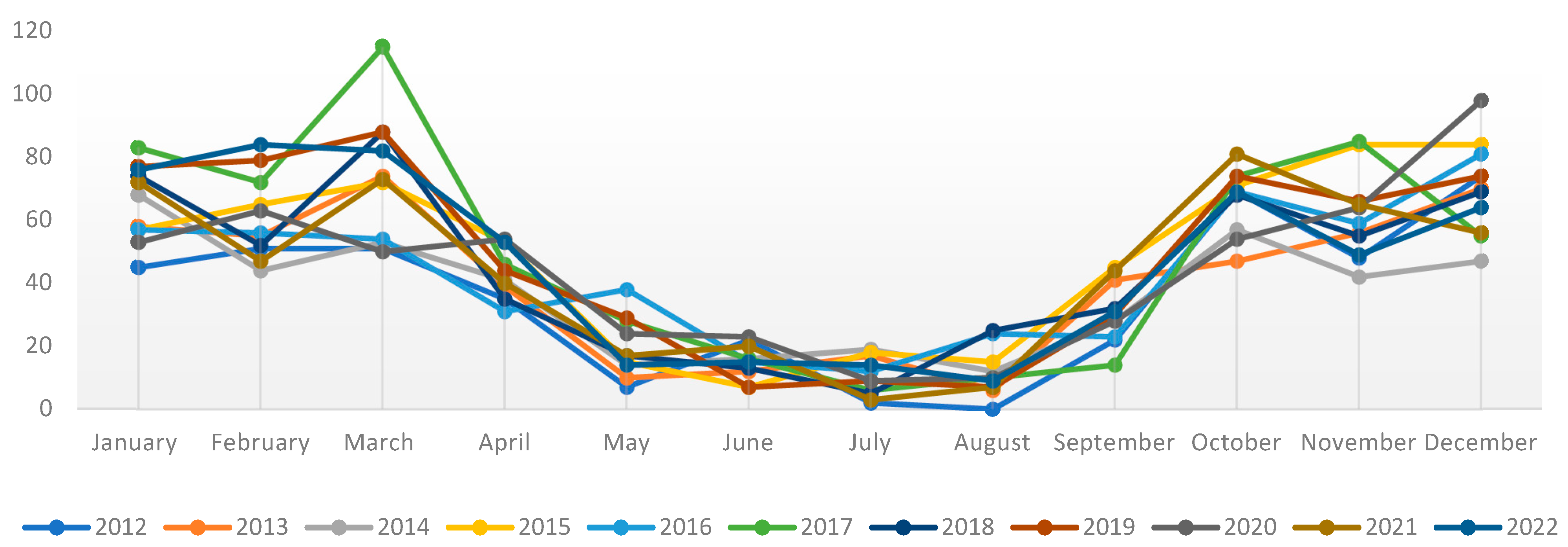
According to Teru and Okabe [30], the faults that occur in Japanese distribution lines are mainly caused by electrical discharges. They are the leading causes of ESIs in China, Japan, and Malaysia [28]. In this sense, Figure 1 shows the monthly average number of disturbances caused by electrical discharges over ten years in Brazil. It is observed that there are more discharges in the first and fourth quarters of the year because this period is more humid and rainy [7].
3. Spatial Data Analysis
An SDA aims to measure properties and relationships considering the phenomenon of spatial location. In this way, the geographic space is incorporated into the study; thus, there is a visual perception via the spatial distribution of the problem under analysis [31].
3.1. Exploratory Spatial Data Analysis
An ESDA is a graphical presentation of georeferenced data on thematic maps or heat maps. An ESDA is a set of techniques to describe and explore spatial or georeferenced data [32]. In this context, a series of metrics derived from descriptive statistics are incorporated; thus, one can identify spatial patterns and formulate hypotheses related to data distribution in geographical space [31,33]. An ESDA is the first step toward a study in SDAs.
3.1.1. Spearman’s Correlation Coefficient
Spearman’s global correlation coefficient in (1) estimates whether two variables are associated; additionally, they do not need to be linearly associated [31].
The coefficient is obtained by arranging the values of two variables in ascending (or descending) order, replacing each original value with a positive integer that represents the ordinal position of the original value in the data series. This correlation coefficient is calculated via (1):
where is the number of CTs; is the square of the difference between the ordinal position of two variables in the same CT.
This coefficient varies in the range [−1, 1], where a positive correlation coefficient implies a directly proportional relationship between the variables, while a negative coefficient implies an inversely proportional relationship.
Additionally, Spearman’s coefficient is not sensitive to asymmetries in the data distribution or outliers. It indicates the degree of dependence between two variables and is an important tool for formulating hypotheses about spatial dependence and cause-and-effect relationships.
Finally, it is worth mentioning that Spearman’s coefficient is a global metric whose influence on the neighborhood is not considered. In contrast, the next section presents local metrics, where the influence of neighboring CTs is represented by a spatial weighting matrix.
3.2. Spatial Analysis with Data Aggregated by Regions
This study is associated with an SDA using data aggregated by regions. It consists of methods that allow for the analysis of georeferenced data whose location is associated with areas delimited by polygons. It is applied to address events aggregated by municipalities, neighborhoods, or CTs, where the exact location of events is unavailable; however, an aggregated value by area is available. The visualization of data aggregated by regions is usually performed through thematic maps with the spatial pattern phenomenon under study [16,34,35].
With data aggregated by areas, an SDA allows for the use of public information by the Brazilian Institute of Geography and Statistics (IBGE). The IBGE does not disclose the private data of the individuals interviewed for confidentiality reasons. These data are grouped into small areas or polygons called CTs, whose area is a function of population density: CTs with a higher population density have a smaller area and vice versa.
3.2.1. Weighting Matrix
Studies in the specialized literature that apply SDA techniques commonly belong to epidemiology, botany, criminology, and mineral resources’ prospecting. In these fields of study, there is a typical neighborhood structure based on spatial proximity or Euclidean distance among the centroids of areas; closer areas have more significant influence than more distant areas [36]. This neighborhood structure based on spatial proximity among areas is also applied in our study. Numerous other neighborhood structures are based on spatial proximity among areas evaluated in [37].
In this context, a spatial weighting matrix (SWM) is formed using weights , where the degree of spatial relationship or spatial dependence between the variables observed in the areas and is estimated. An SWM is an essential tool for GW modeling. Three key elements must be considered for SWM building: distance type, kernel function, and bandwidth [38,39].
The SWM is a symmetric matrix built for a set of areas , where, from each element , the spatial relationship or spatial dependence between the variables observed in and areas are estimated.
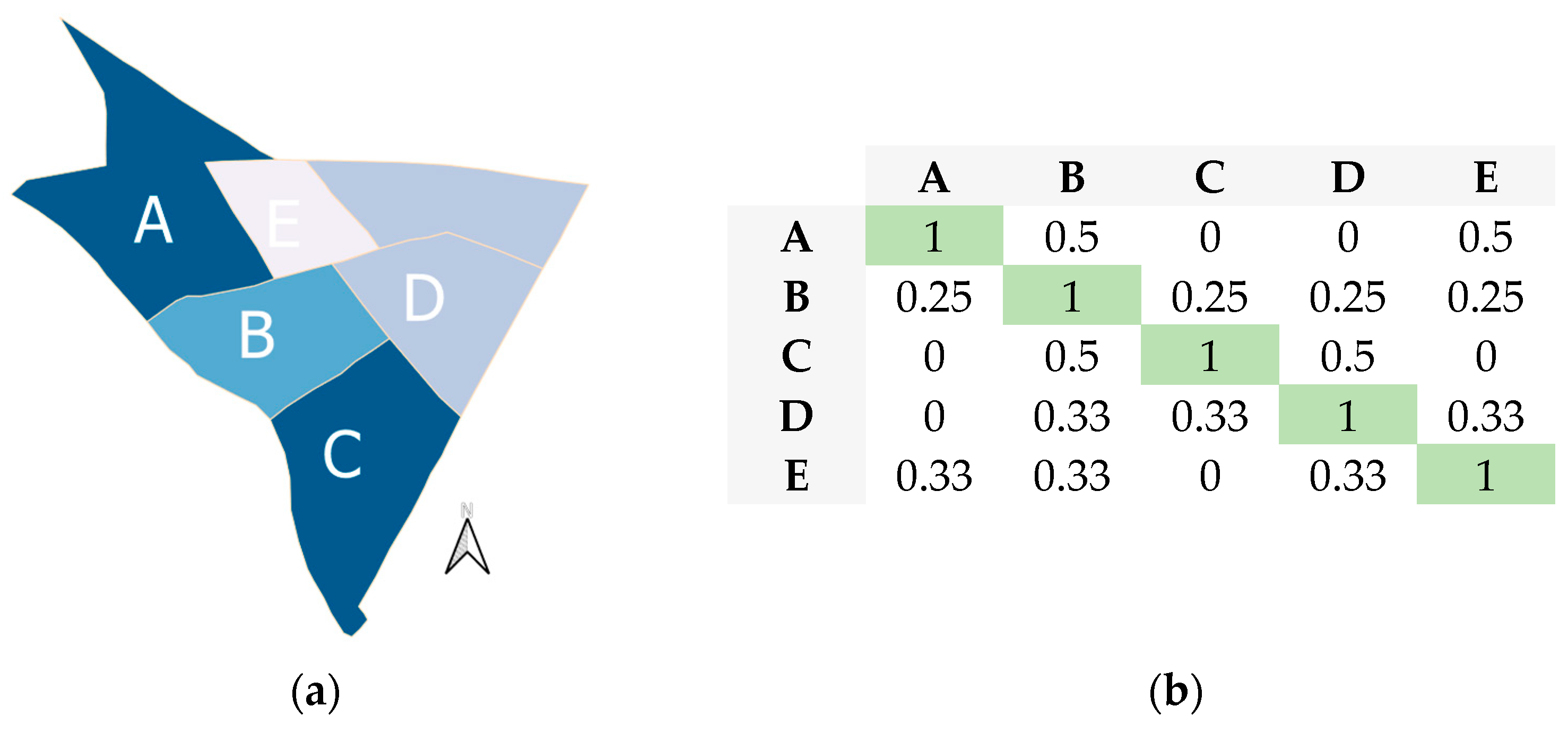
Figure 2 shows an illustrative example of obtaining a weighting matrix . In Figure 2a, there is a city with five CTs (, , , and ); on the other hand, in Figure 2b, there is a weighting matrix for a city with CTs and whose obtaining rule is according to (2). The CT has borders in common with two other CTs: and . Therefore, the total number of borders of CTs for is equal to two. Thus, the weighting matrix elements, (weighting between and ) and (weighting between and ), are equal to according to (2). Other CTs do not have borders in common with ( and for example); therefore, they have zero weighting: and .
3.2.2. Geographically Weighted Statistics Metrics
Geographically weighted models (GWMs) are techniques belonging to non-stationary spatial statistics, which incorporate local spatial relationships into their structure intuitively and explicitly [38,40]. Their application is suitable for situations where the spatial data need to be better described using a local model since they enable the estimation and mapping of each location in the geographical space under study. GWMs’ outputs are commonly mapped to provide a helpful tool that usually precedes a more sophisticated statistical analysis [38].
Spatial weighting functions are crucial elements in GW modeling, whose objective is quantifying the spatial relationship or spatial dependence between the observed variables via SWM [38].
In this context, in our study, SWM elements are obtained via a Gaussian kernel application in (3) and shown in Figure 3. It is a monotonic decreasing function of the distance among centroids of areas and . These functions have a parameter for the bandwidth, which controls their decay rate [34,38].
For example, Figure 3 shows the most conventional kernel function or weighting function from Gollini et al. [38]: the Gaussian kernel. It is obtained using (3) with an arbitrary bandwidth .
where represents the distance between the centroids of areas and , and is the bandwidth parameter.
It is worth pointing out that kernel the function selection is performed empirically. The Gaussian kernel is chosen because it follows Tobler’s first law, where the weighting between nearby CTs is greater than for distant CTs [36]. Furthermore, as shown in Figure 3, the Gaussian kernel is a continuous function with a smooth decay. Additionally, the decay rate is regulated through a bandwidth parameter . Other kernel functions with characteristics analogous to the Gaussian kernel could be applied.
A GW local summary statistic can be obtained from a spatial data set. Therefore, from the attributes and at any point , the following metrics can be obtained through (4)–(7): mean GW, standard deviation GW, Pearson’s correlation coefficient GW, and covarianceGW, respectively [38,41].
where is an element of SWM .
4. Results and Discussion
In this study, the spatial regression terminology is applied where there is a dependent or study variable whose distribution in geographic space is partially explained through a set of independent or explanatory variables. In our study, the dependent variable consists of a percentage of damaged distribution transformers that resulted in steady-state failures.
According to [42], the power utility of Paraná State, Brazil (COPEL), presented an annual failure rate of 1.2% in distribution transformers, where electric discharges caused 30% of these occurrences.
In this sense, the independent or explanatory variable analyzed is the surface density of electric discharges per km2. They are associated with faults in distribution feeders. It is worth pointing out that all transformers and all-electric discharges in the city under study were georeferenced; their geographic coordinates were known, making it possible to apply an SDA.
4.1. Case Study in A Brazilian City
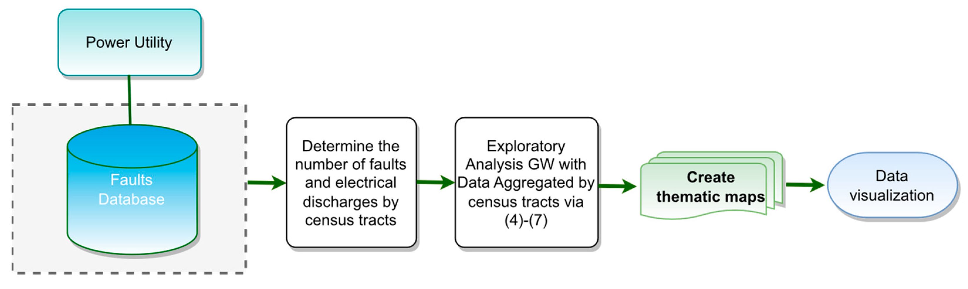
This work performs an exploratory spatial data analysis to evaluate how electric discharges influence some city regions more vulnerable to steady-state faults. In this sense, Figure 4 shows an overview of the main steps of our study: the (1) acquisition of georeferenced data (damaged distribution transformers and electric discharges), (2) exploratory analysis of spatial data, and (3) display of the results in thematic maps.
The power utility applied in the simulations had a real feeder located in São Paulo State, Brazil. The simulations used QGIS version 3.30 and R software version 4.1.2 [37]. QGIS is a GIS that allows for the visualization, editing, and analysis of spatial data. QGIS allows for the checking, processing, previewing, updating, and presentation of spatial data. Different types of data can be displayed through maps, where it is possible to understand patterns, trends, and relationships [15].
On the other hand, R is a programming language and free statistical and graphical computing software. It contains many libraries or packages for numerical analysis, such as the GWmodel version 2.3.1 applied in this study. Unlike QGIS, R was not initially created as a GIS; however, it can perform functions like a GIS.
All simulations in this study were performed on a computer with a Windows operating system; an Intel Core i7 processor, 1.8–2.3 GHz, 64-bit; and 16 GB of RAM.
4.2. Database Description
In this section, the variables electrical discharge density () and the percentage of permanent faults in distribution transformers by regions () are evaluated because electrical discharges can make some city regions more vulnerable to faults. and are variables obtained in small areas called CTs. CTs show the public demographic census data produced by IBGE because individual data are confidential.
Consider a of the city under analysis with , where corresponds to the number of CTs. The dependent or study variable is shown in (8). It is obtained from the ratio between the number of permanent faults per that caused faults in power distribution transformers and the total number of transformers in represented by . represents the probability of faults in the transformer per CT. Thus, the number of failures in transformers of is approximately proportional to its total number of transformers. It is noteworthy that the faults in our study are associated with transformers because they are georeferenced:
The surface density of electrical discharges () is an independent or explanatory variable, and it is expressed in (9). It is the ratio between the number of electrical discharges and the of area per km2. The variable obtained is more effective than the total number of electrical discharges by CTs because the number of electrical discharges that reach a CT is approximately proportional to its area.
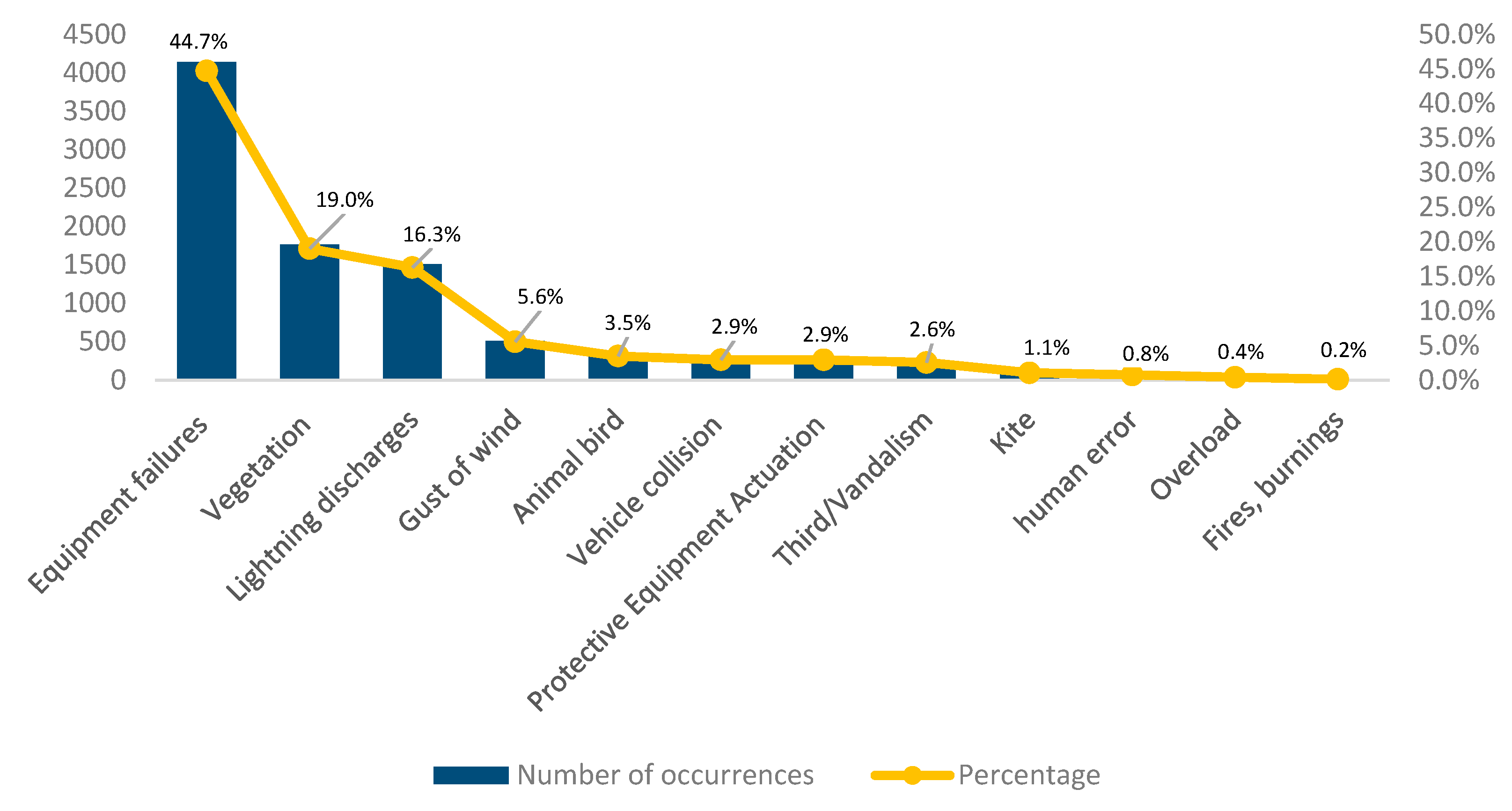
Figure 5 shows the main reasons that caused 9266 ESIs in more than one minute in a Brazilian city over four years. According to Figure 1 and Figure 5, weather conditions are the leading causes of interruptions in the utility grid. Figure 5 shows that meteorological conditions such as wind gusts and electrical discharges accounted for 21.9% of ESIs.
However, it is worth noting that Figure 5 shows numerical values from the power utility database without a refined treatment. Thus, technicians in the field identified the percentages associated with the factors responsible for ESIs without further investigation. For example, the leading causes of ESIs were “equipment failures”, with an occurrence of 44.7%. However, this is a “black box” because equipment failures can be caused by numerous factors such as equipment obsolescence, adverse weather conditions (rains, wind gusts, electrical discharges), overload, clandestine connections, or human failures. In this sense, the overview of the numerous factors responsible for ESIs is more important than the numerical values shown in Figure 5.
4.3. Exploratory Spatial Data Analysis
4.3.1. Electrical Discharges
Electrical discharges occasionally reach the utility grid; consequently, they cause disturbances and ESIs. Figure 6 shows a monthly distribution of 2036 electrical discharges that occurred in the city under study over four years. Table 2 shows some descriptive statistics metrics by CTs. From Table 2, each CT experiences between one and two electrical discharges by year on average. However, a single CT was the target of 40 electrical discharges in 2011.
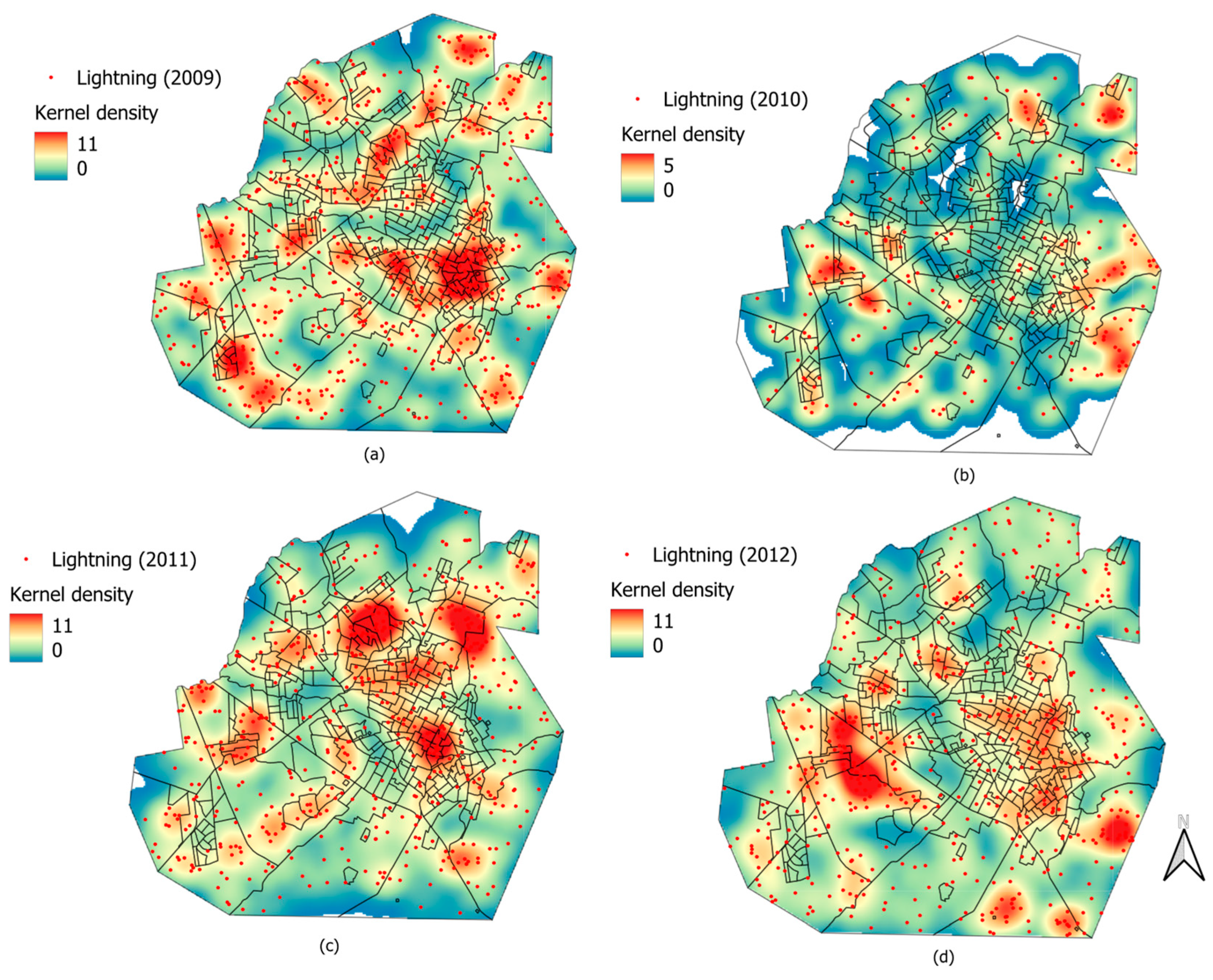
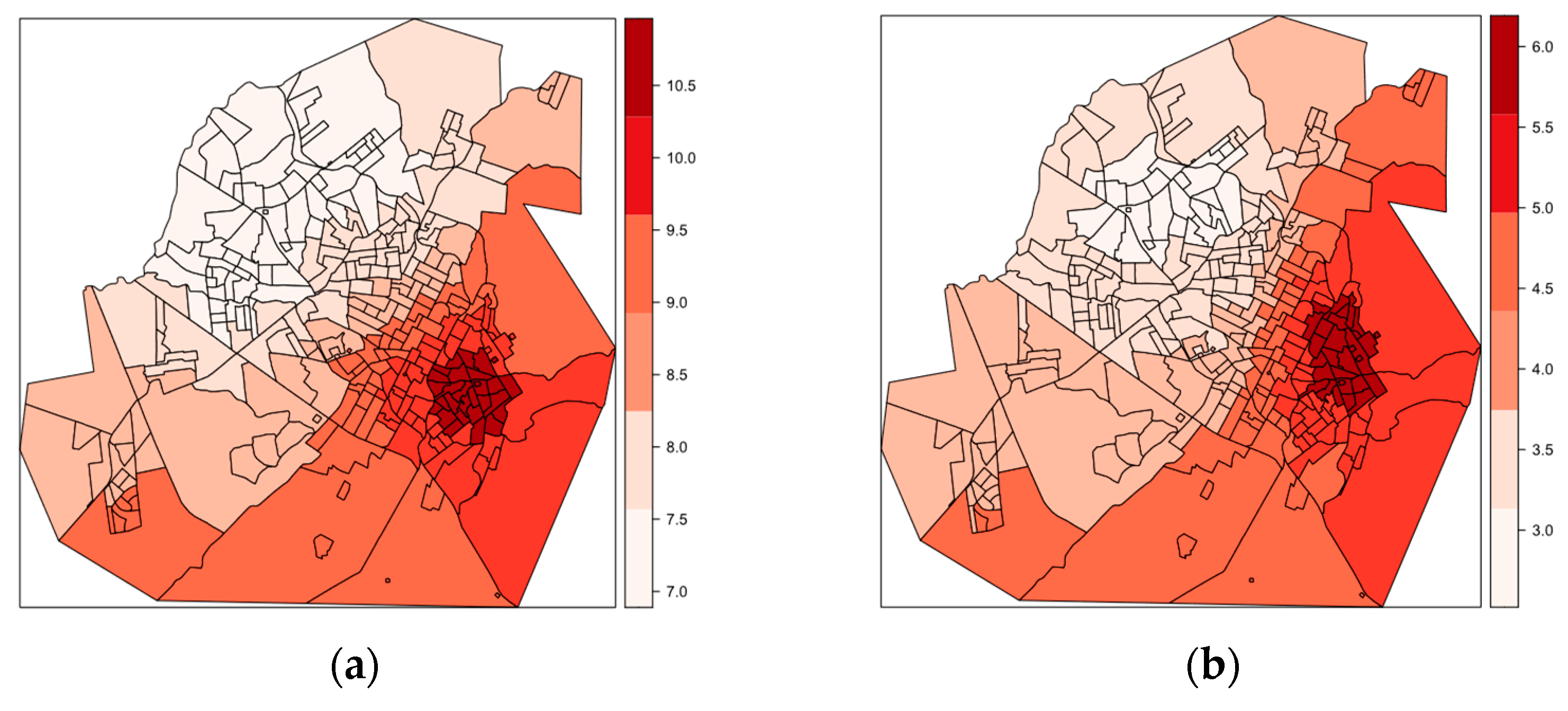
Figure 7a–d show the heat maps obtained using the Gaussian kernel density considering the electrical discharge distribution for the years 2009, 2010, 2011, and 2012, respectively. The Gaussian kernel is based on electrical discharge clustering based on a predefined distance called bandwidth. Therefore, CTs with high concentrations of electrical discharges (indicated by red regions) have high Gaussian kernel values. The maximum Gaussian kernel value in 2010 corresponds to approximately half of the value observed in other years, for example. Therefore, this variation indicates a heterogeneous distribution of electrical discharges over the years.
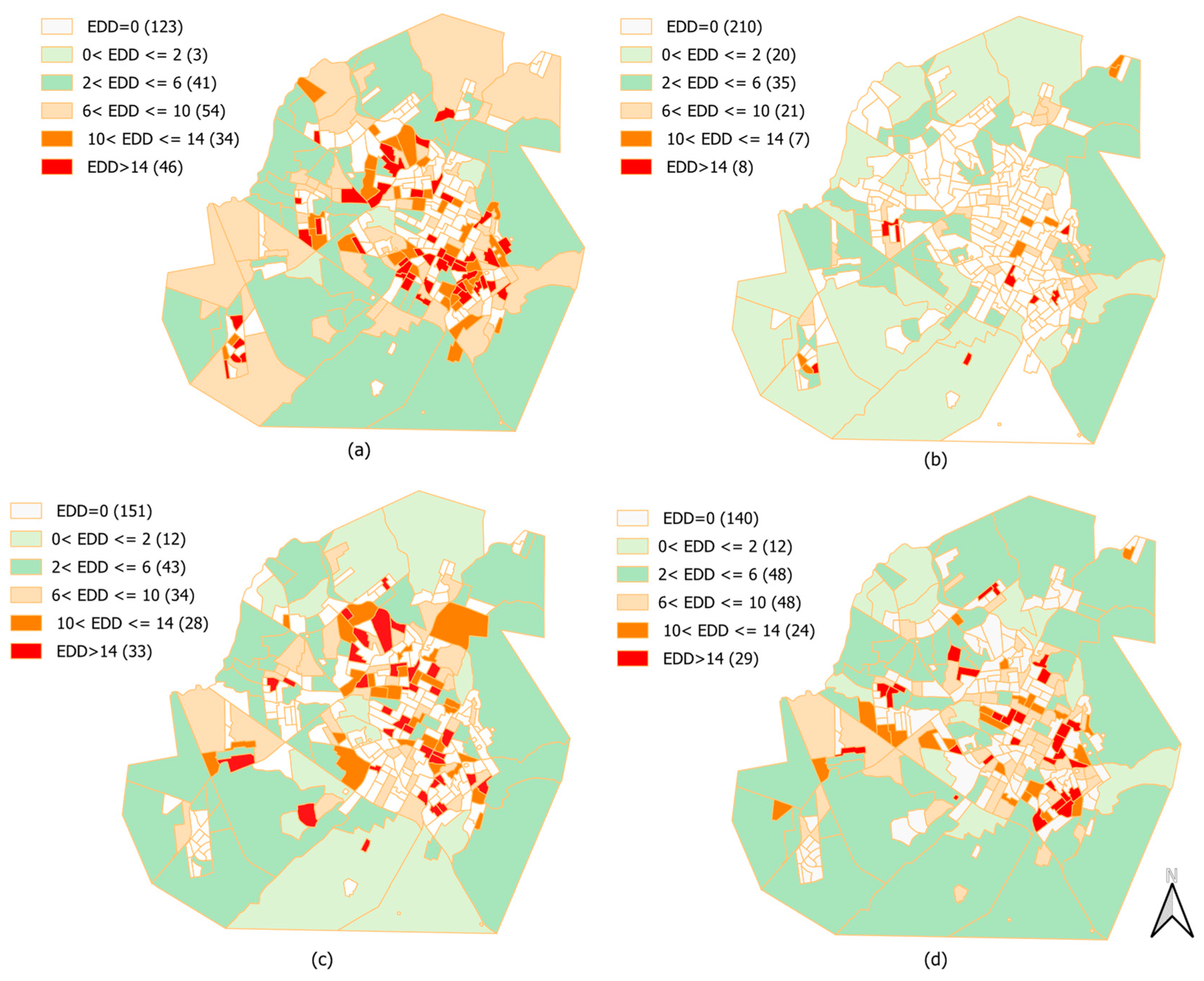
The variable considers the total area of each CT in km2. In many cases, the number of electrical discharges in a CT is proportional to its area. Figure 8a–d show thematic maps for over the years 2009, 2010, 2011, and 2012, respectively. The numbers in parentheses indicate the CTs whose is in the designated range. For example, in Figure 8a, which corresponds to the in 2009, it is observed that 41 CTs have an with a value between 2 and 6 electrical discharges per km2. Most of these CTs belong to the city’s periphery and are represented in light green.
According to Figure 8, the EDD has a similar pattern for all years analyzed. CTs with a high EDD belong to the central regions and move toward the center-southeast and center-northwest of the city. There is an exception in Figure 8b. According to Table 2, 2010 is an atypical year (outlier) with few rains and electrical discharges. The regions with a high EDD (central, northwest, and southeast) are more densely urbanized and have many elevated structures such as buildings, antennas, and tree vegetation that attract electrical discharges. Overhead lines also attract electrical discharges; thus, they have protective equipment to deal with them. On the other hand, CTs located on the city’s periphery and, therefore, close to rural areas show a reduced EDD. These CTs contain extensive flat areas with open fields.
4.3.2. Number of Faults in Transformers by Regions
The number of faults in transformers is the dependent or study variable. This work covers 3794 interruptions caused by distribution-transformer failures. This approach is adopted because transformers are georeferenced, and this is a condition for using SDA techniques.
Table 3 shows metrics of descriptive statistics applied to the annual number of interruptions by CTs caused by faults in power distribution transformers from 2009 to 2012. There were three yearly interruptions by CT on average. However, there were 42 interruptions in a single CT caused by transformer failures in 2009.
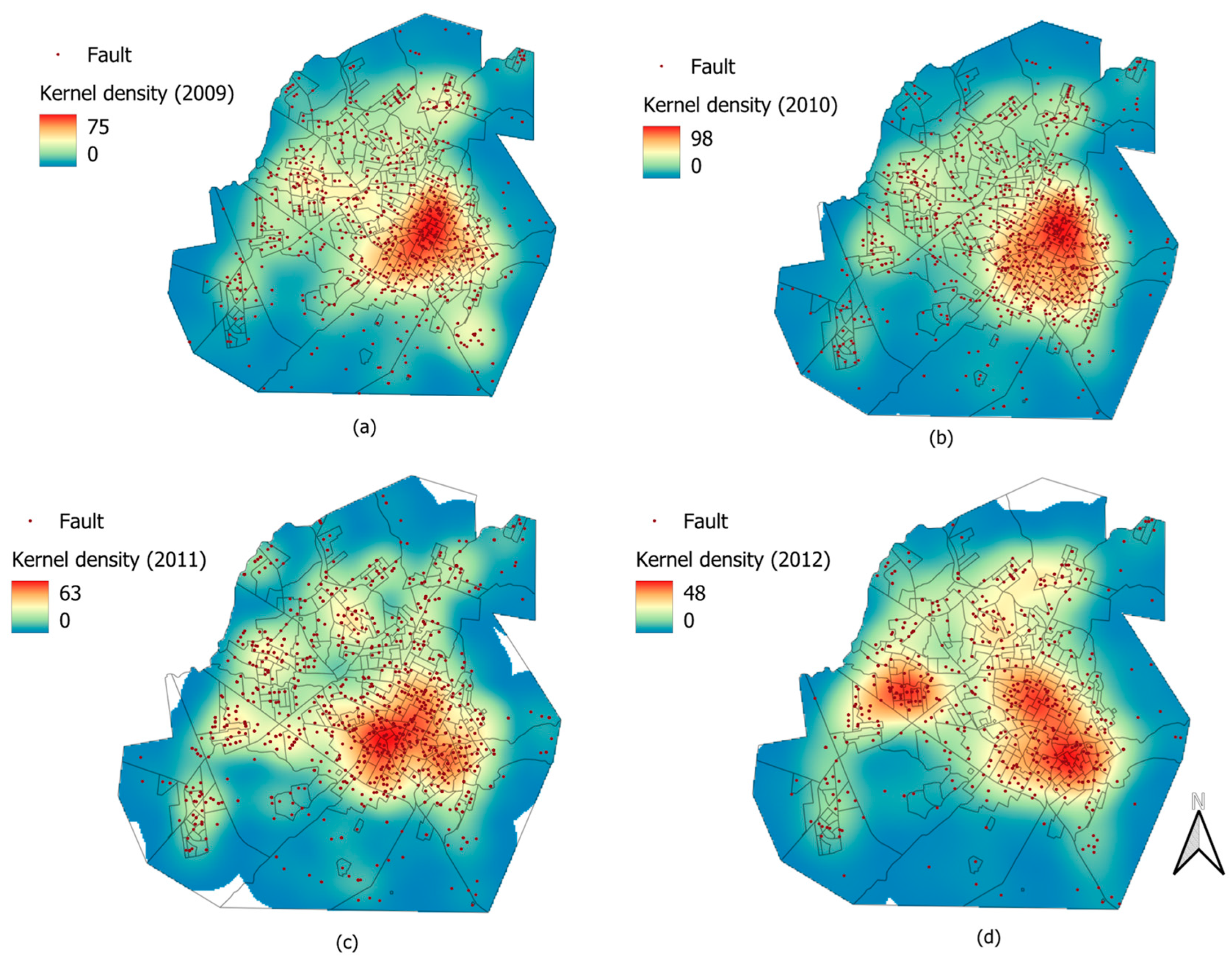
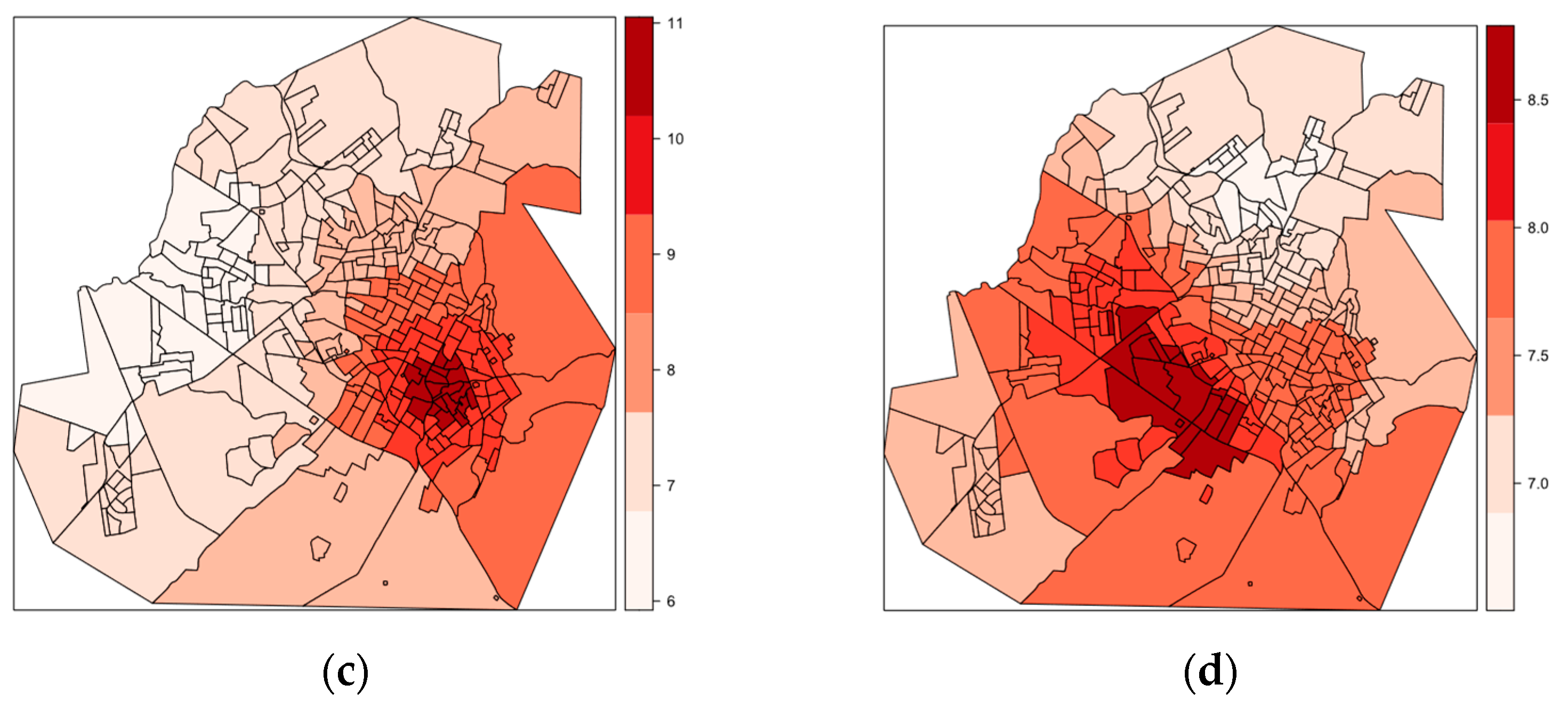
Figure 9a–d show the heat maps where the interruptions in distribution transformers that occurred in 2009, 2010, 2011, and 2012 are represented. The main objective is to visualize the high concentration of interruptions in transformers in some city areas. The heat maps for all years have a similar pattern with a high fault concentration in the city’s central region. This region has a high population density and, therefore, has many transformers. Figure 9c shows the heat map for the year 2011, with warm areas in the center-southeast direction. Finally, Figure 9d shows the heat map for the year 2012, where there is a significant cluster of distribution transformer faults in the western, center, and southeast regions.
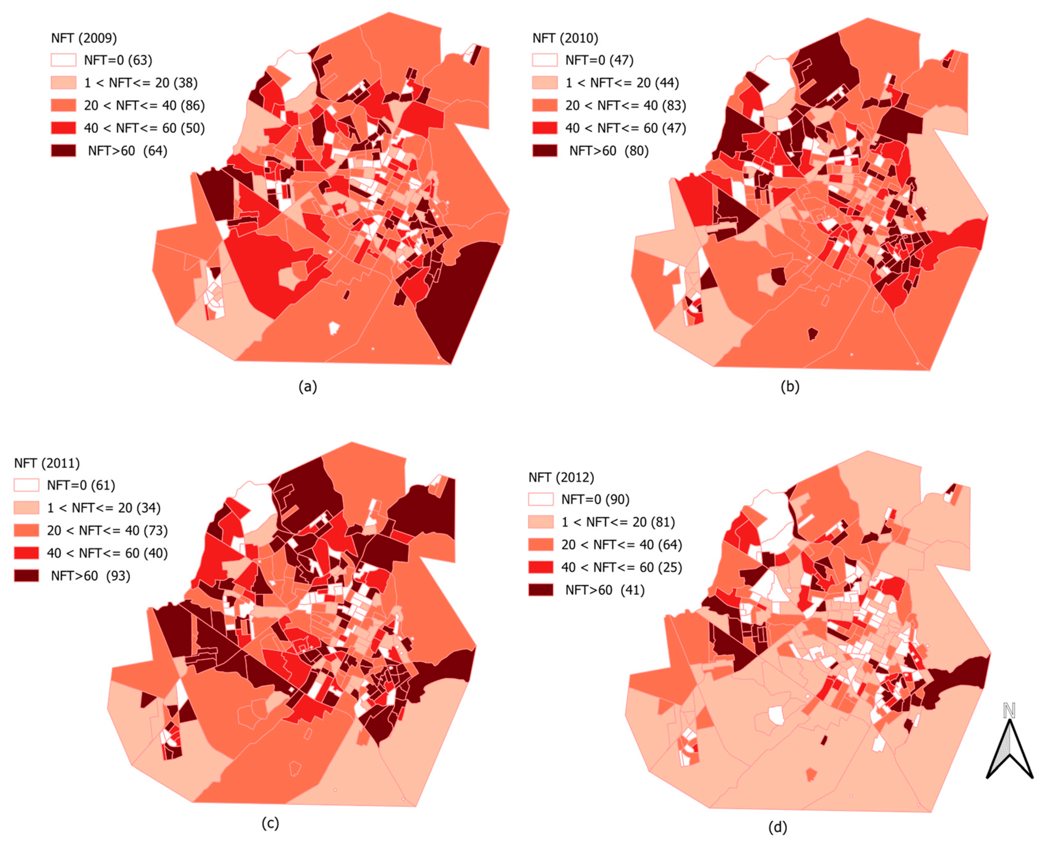
In this sense, Figure 10a–d show thematic maps for the NFT dependent variable for the years 2009, 2010, 2011, and 2012, respectively. The maps visually represent interruptions, considering the total number of transformers installed in each CT. There is a contrast between Figure 9 and Figure 10. Figure 9 shows a fault distribution pattern with a significant concentration in the central region. On the other hand, Figure 10 shows a variation in trends over the years studied.
It is noteworthy that Figure 10 shows information in parentheses with the total number of CTs whose NFT is within the indicated range. For example, Figure 10a shows 86 CTs with , where most of the CTs have NFT in that range for all years evaluated.
In Figure 10a, there are 64 CTs with a high . Most are in the southeast, west, and north regions. In Figure 10b, there are 80 CTs with a high . The southeast and west regions contain some CTs with a high NFT, and other CTs appear in the northwest region. Figure 10c has the largest number of CTs with a high NFT, being 93 CTs. The southeast, west, and northwest regions contain many CTs with a high , and other CTs appear in the northeast and central regions. Lastly, Figure 10d has the smallest number of CTs with a high NFT: there are 41 CTs, and the majority are in the east, west, and northwest regions. Certainly, in 2012, the distributor performed the maintenance or replacement of many damaged transformers located in CTs with many faults.
According to Figure 10, there are some CTs with a high NFT located in peripheral city regions. On the other hand, these regions have a low in Figure 8. Therefore, a preliminary assessment indicates that there are possibly other local variables that influence the high NFT in these regions.
In this context, peripheral regions close to rural regions are fire targets. However, we cannot conclude that the is high in peripheral regions of the city due to fires. Further studies should confirm or refute that hypothesis.
4.3.3. Geographically Weighted Summary Statistics
Spearman’s correlation global coefficient between the and is shown in Table 4 for the years 2009 to 2012 according to (1). The and have a moderate positive global correlation for all years analyzed. Thus, a cause-and-effect relationship may exist between these variables; therefore, an increase in the causes an increase in the . Additional investigations must be performed to confirm or refute this hypothesis.
In contrast to local metrics, global metrics do not consider the influence of neighboring CTs, whose influence is represented by SWM. Thus, the correlation absence at the global level does not imply the correlation absence at the local level [31,37]. Therefore, global and local correlations can present different results because the correlation coefficient at a global level represents all CTs with a single numerical value.
Therefore, for a more detailed analysis, a GW local exploratory analysis is performed considering the influence of neighboring CTs. In this sense, this section presents thematic maps as the result of applying the GW metrics in (4)–(7). The neighborhood structure among the nth CTs influences these GW metrics. The neighborhood structure is represented by the weighting matrix which is constructed from the Gaussian kernel in (3) and represented in Figure 3.
The neighborhood structure in this study follows Tobler’s notion of spatial dependence, which states the first law of geography where all things are similar; however, things closer look more than distant things [36].
In this sense, the weighting assigned by the Gaussian kernel is inversely proportional to the Euclidean distance between the CT centroids. Thus, as the distance between CTs and is reduced, the weighting between them increases. The elements belong to the weighting matrix , and it represents the neighborhood structure in an urban area of a Brazilian city with CTs.
Therefore, if a CT has a high number of electrical discharges, it is likely that nearby CTs will show this same characteristic. On the other hand, if a CT has feeders with many ESIs, nearby CTs are expected to have this same problem because they share the same power grid. Therefore, the neighborhood structure based on Euclidean distance among CTs is suitable for estimating areas vulnerable to faults.
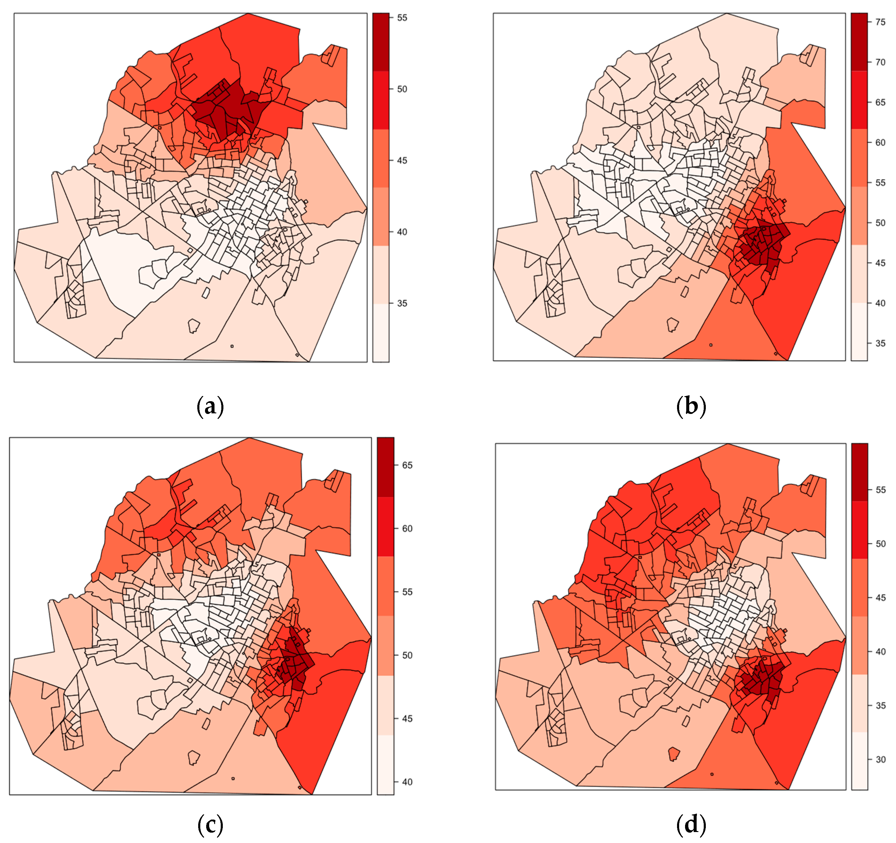
Figure 11a–d show the GW standard deviation for the independent variable for the years 2009, 2010, 2011, and 2012, respectively. Figure 11a,c show high local variability for the central and southeastern regions. Figure 11b shows high local variability for the central-east region. Finally, Figure 11d shows high local variability for the central-eastern region. A high local variability indicates that there are nearby CTs that present very different values. As shown in Figure 11, it is worth highlighting the high local variability in regions around the central area. It contains buildings and tree vegetation that attract electrical discharges.
On the other hand, Figure 12a–d show the GW standard deviation for the dependent variable for the years 2009, 2010, 2011, and 2012, respectively. Figure 12a shows high local variability for the northern regions. Figure 12b shows high local variability for the southeast region, and finally, Figure 12c,d show high local variability for the southeast and northwest regions. It is worth highlighting that there is a change in regions with greater local variability that is more pronounced for the than the over the years. Field teams work continuously to maintain and replace damaged transformers; therefore, there is greater variation in the than the by CTs over the years.
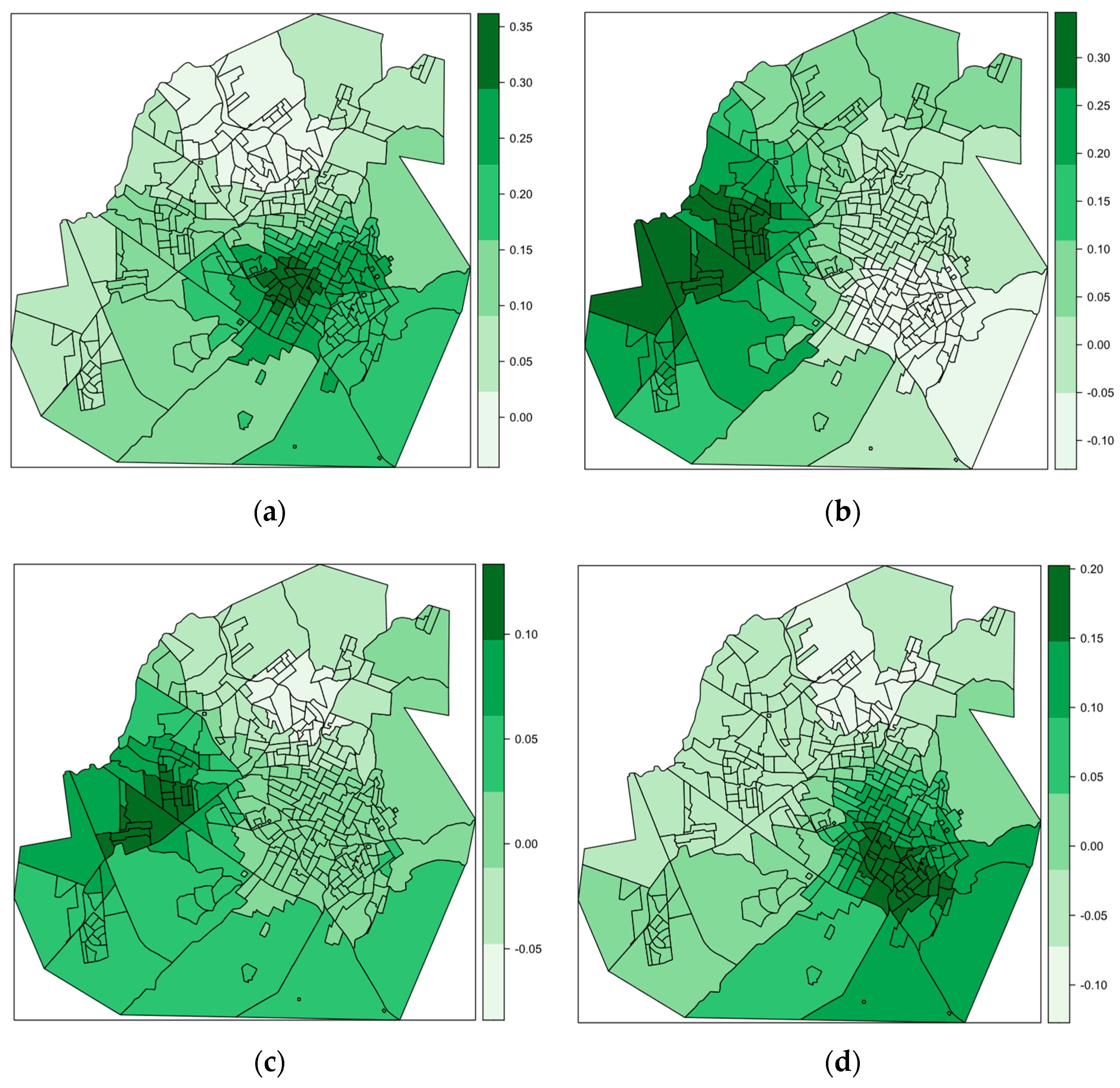
Lastly, Figure 13a–d show a local correlation GW between the dependent variable and the independent variable for 2009 to 2012, respectively. There is a non-stationary relationship between the and variables with a moderate GW local correlation in the central (Figure 13a,d) and west (Figure 13b,c) regions.
The positive correlation means that, in these regions, the and are directly proportional variables. Therefore, there is first a numerical indication that electrical discharges are associated with ESIs in power grid transformers in these regions.
The non-stationary relationship between the and indicates that a global spatial regression model would not be suitable for estimating regions vulnerable to faults; on the other hand, a local regression model would be better suited to represent non-stationarity at the local level.
It is worth highlighting that GWEA is performed with an adaptive bandwidth where the influence of the 45 closest CTs is considered for the analysis of each CT. This closest CT value corresponds to 15% of the total CTs in the city under study [38].
5. Conclusions
In this study, a crucial step was performed that preceded the estimating of census tracts (CTs) vulnerable to faults: the geographically weighted (GW) exploratory spatial data analysis (ESDA). Essential for this analysis was the availability of georeferenced real data: the dependent variable, number of faults in distribution transformers () by census tracts (CTs) and the independent or explanatory variable, electrical discharges density ().
An ESDA was performed using metrics of GW statistics with a visual presentation of variables in the city’s geographical space. The GW statistics summarily demonstrated the spatial variability between the and variables.
The GW correlation showed a moderate positive correlation between the and in the central (in 2009 and 2012) and in the west (in 2010 and 2011) regions. Therefore, electrical discharges are associated with the power grid faults in these regions.
It is worth mentioning a limitation of this study: only faults in power distribution transformers were considered, which was because the geographical coordinates of the equipment were known.
The ESDA performed in this study is vital for implementing more sophisticated mathematical models in future studies to estimate regions vulnerable to faults. Furthermore, incorporating other variables, such as tree vegetation, will provide greater robustness to future analysis.
Author Contributions
Conceptualization, A.S.S. and L.T.F.; methodology, A.S.S. and L.T.F.; software, A.S.S. and L.T.F.; validation, A.S.S., L.T.F., M.L.M.L. and C.R.M.; formal analysis, A.S.S., L.T.F., M.L.M.L. and C.R.M.; investigation, A.S.S.; resources, C.R.M.; data curation, A.S.S.; writing—original draft preparation, A.S.S. and L.T.F.; writing—review and editing, A.S.S., L.T.F., M.L.M.L. and C.R.M.; visualization, A.S.S.; supervision, C.R.M.; project administration, C.R.M.; funding acquisition, C.R.M. All authors have read and agreed to the published version of the manuscript.
Funding
This research was funded by Coordination for the Improvement of Higher Education Personnel (CAPES), Financing Code 001, and the National Council for Scientific and Technological Development (CNPq) Agency—Brazil.
Data Availability Statement
The data presented in this study are available on request from the corresponding author. The data are not publicly available because the authors are not allowed to publish them publicly.
Conflicts of Interest
The authors declare no conflict of interest.
References
- Zhou, Q.; Li, X.; Liao, J.; Xiong, T. Power failure risk assessment and management based on stochastic line failures in distribution network including distributed generation. IEEJ Trans. Electr. Electron. Eng. 2018, 13, 1303–1312. [Google Scholar] [CrossRef]
- Gururajapathy, S.S.; Mokhlis, H.; Illias, H.A. Fault location and detection techniques in power distribution systems with distributed generation: A review. Renew. Sustain. Energy Rev. 2017, 74, 949–958. [Google Scholar] [CrossRef]
- Mikropoulos, P.N.; Tsovilis, T.E. Statistical Method for the Evaluation of the Lightning Performance of Overhead Distribution Lines. IEEE Trans. Dielectr. Electr. Insul. 2013, 20, 202–211. [Google Scholar] [CrossRef]
- Wang, C.; Zhang, T.; Luo, F.; Li, P.; Yao, L. Fault incidence matrix based reliability evaluation method for complex distribution system. IEEE Trans. Power Syst. 2018, 33, 6736–6745. [Google Scholar] [CrossRef]
- Leite, J.B.; Mantovan, J.R.S.; Dokic, T.; Chen, Q.Y.; Kezunovic, M. Failure Probability Metric by Machine Learning for Online Risk Assessment in Distribution Networks. In Proceedings of the 2017 IEEE PES Innovative Smart Grid Technologies Conference-Latin America (ISGT Latin America), Quito, Ecuador, 20–22 September 2017; pp. 1–6. [Google Scholar]
- Souza, F.A.; Castoldi, M.F.; Goedtel, A. A cascade perceptron and Kohonen network approach to fault location in rural distribution feeders. Appl. Soft Comput. 2020, 96, 106627. [Google Scholar] [CrossRef]
- National Electric System Operator, “Supply Quality”, ONS. Available online: https://www.ons.org.br/ (accessed on 1 July 2023). (In Portuguese).
- da Silva Santos, A.; Faria, L.T.; Lopes, M.L.M.; Lotufo, A.D.P.; Minussi, C.R. Efficient Methodology for Detection and Classification of Short-Circuit Faults in Distribution Systems with Distributed Generation. Sensors 2022, 22, 9418. [Google Scholar] [CrossRef] [PubMed]
- Zhang, C.; Wang, J.; Huang, J.; Cao, P. Detection and classification of short-circuit faults in distribution networks based on fortescue approach and softmax regression. Int. J. Electr. Power Energy Syst. 2020, 118, 105812. [Google Scholar] [CrossRef]
- Chaitanya, B.K.; Yadav, A. An intelligent fault detection and classification scheme for distribution lines integrated with distributed generators. Comput. Electr. Eng. 2018, 69, 28–40. [Google Scholar] [CrossRef]
- Elnozahy, M.S.; El-Shatshat, R.A.; Salama, M.M.A. Single-phasing detection and classification in distribution systems with a high penetration of distributed generation. Electr. Power Syst. Res. 2016, 131, 41–48. [Google Scholar] [CrossRef]
- Dehghani, M.; Khooban, M.H.; Niknam, T. Fast fault detection and classification based on a combination of wavelet singular entropy theory and fuzzy logic in distribution lines in the presence of distributed generations. Int. J. Electr. Power Energy Syst. 2016, 78, 455–462. [Google Scholar] [CrossRef]
- Yuan, J.; Jiao, Z. Faulty feeder detection based on image recognition of current waveform superposition in distribution networks. Appl. Soft Comput. 2022, 130, 109663. [Google Scholar] [CrossRef]
- AL-Sakkaf, A.-S.A.; AL-Ramadan, B.M. Applications of GIS in Electrical Power System; King Fahd University of Petroleum and Minerals: Dhahran, Saudi Arabia, 2013; pp. 1–6. [Google Scholar]
- Shafiullah, M.; Rahman, S.M.; Mortoja, M.G.; Al-Ramadan, B. Role of spatial analysis technology in power system industry: An overview. Renew. Sustain. Energy Rev. 2016, 66, 584–595. [Google Scholar] [CrossRef]
- Câmara, G.; Carvalho, M.S.; Cruz, O.G.; Correa, V. Spatial Analysis of Areas; Editora EMBRAPA: Brasília, Brazil, 2004. (In Portuguese) [Google Scholar]
- Abdulrahman, I.; Radman, G. Power system spatial analysis and visualization using geographic information system (GIS). Spat. Inf. Res. 2019, 28, 101–112. [Google Scholar] [CrossRef]
- Chen, C.; Kezunovic, M. Fuzzy Logic Approach to Predictive Risk Analysis in Distribution Outage Management. IEEE Trans. Smart Grid 2016, 7, 2827–2836. [Google Scholar] [CrossRef]
- Goerdin, S.A.V.; Smit, J.J.; Mehairjan, R.P.Y. Monte Carlo simulation applied to support risk-based decision making in electricity distribution networks. In Proceedings of the 2015 IEEE Eindhoven PowerTech, PowerTech 2015, Eindhoven, The Netherlands, 29 June–2 July 2015; Institute of Electrical and Electronics Engineers Inc.: Piscataway, NJ, USA, 2015. [Google Scholar] [CrossRef]
- Muñoz, D.S.; Garcia, J.L.D. GIS-based tool development for flooding impact assessment on electrical sector. J. Clean. Prod. 2021, 320, 128793. [Google Scholar] [CrossRef]
- Bernstein, A.; Bienstock, D.; Hay, D.; Uzunoglu, M.; Zussman, G. Power Grid Vulnerability to Geographically Correlated Failures–Analysis and Control Implications. In Proceedings of the IEEE INFOCOM 2014-IEEE Conference on Computer Communications, Toronto, ON, Canada, 27 April–2 May 2014; IEEE: Piscataway, NJ, USA, 2014; pp. 2634–2642. [Google Scholar]
- Handayani, K.; Filatova, T.; Krozer, Y. The vulnerability of the power sector to climate variability and change: Evidence from Indonesia. Energies 2019, 12, 3640. [Google Scholar] [CrossRef]
- Mortensen, L.K.; Shaker, H.R.; Veje, C.T. Relative fault vulnerability prediction for energy distribution networks. Appl. Energy 2022, 322, 119449. [Google Scholar] [CrossRef]
- Albasri, F.A.; Zaki, A.Z.; Al Nainoon, E.; Alawi, H.; Ayyad, R. A Fault Location System Using GIS and Smart Meters for the LV Distribution System. In Proceedings of the 2019 International Conference on Innovation and Intelligence for Informatics, Computing, and Technologies, Sakhier, Bahrain, 22–23 September 2019; IEEE: Piscataway, NJ, USA, 2019; pp. 1–6. [Google Scholar]
- Su, X. Engineering fault intelligent monitoring system based on Internet of Things and GIS. Nonlinear Eng. 2023, 12, 20220322. [Google Scholar] [CrossRef]
- Chen, P.-C.; Dokic, T.; Stokes, N.; Goldberg, D.W.; Kezunovic, M. Predicting weather-associated impacts in outage management utilizing the GIS framework. In Proceedings of the 2015 IEEE PES Innovative Smart Grid Technologies Latin America (ISGT LATAM), Montevideo, Uruguay, 5–7 October 2015; IEEE: Piscataway, NJ, USA, 2015; pp. 417–422. [Google Scholar]
- Xu, Y.; Tong, C.; Xiang, M.; Wang, T.; Xu, J.; Zheng, J. Lightning risk estimation and preventive control method for power distribution networks referring to the indeterminacy of wind power and photovoltaic. Electr. Power Syst. Res. 2023, 214, 108896. [Google Scholar] [CrossRef]
- Sestasombut, P.; Ngaopitakkul, A. Evaluation of a direct lightning strike to the 24 kV distribution lines in Thailand. Energies 2019, 12, 3193. [Google Scholar] [CrossRef]
- Mestriner, D.; de Moura, R.A.R.; Procopio, R.; de Oliveira Schroeder, M.A. Impact of grounding modeling on lightning-induced voltages evaluation in distribution lines. Appl. Sci. 2021, 11, 2931. [Google Scholar] [CrossRef]
- Miyazaki, T.; Okabe, S. Field analysis of the occurrence of distribution-line faults caused by lightning effects. IEEE Trans. Electromagn. Compat. 2011, 53, 114–121. [Google Scholar] [CrossRef]
- Druck, S.; Carvalho, M.S.; Câmara, G.; Monteiro, A.M.V. Spatial Analysis of Geographic Data; Editora EMBRAPA: Brasília, Brazil, 2004. (In Portuguese) [Google Scholar]
- Le Gallo, J.; Ertur, C. Exploratory spatial data analysis of the distribution of regional per capita GDP in Europe, 1980–1995. Pap. Reg. Sci. 2003, 82, 175–202. [Google Scholar] [CrossRef]
- Haining, R. Spatial Data Analysis: Theory and Practice; Cambrigdge University Press: Cambrigdge, UK, 2003; Volume 1. [Google Scholar]
- Faria, L.T.; Melo, J.D.; Padilha-Feltrin, A. Spatial-Temporal Estimation for Nontechnical Losses. IEEE Trans. Power Deliv. 2016, 31, 362–369. [Google Scholar] [CrossRef]
- Ventura, L.; Feliz, G.; Vargas, R.; Faria, L.T.; Melo, J.D. Estimation of Non-Technical Loss Rates by Regions. Electr. Power Syst. Res. 2023, 223, 109685. [Google Scholar] [CrossRef]
- Tobler, W.R. Cellular geography. In Philosophy in Geography; Springer: Berlin/Heidelberg, Germany, 1979; pp. 379–386. [Google Scholar]
- Bivand, R.S.; Pebesma, E.; Gómez-Rubio, V. Applied Spatial Data Analysis with R; Springer: Berlin/Heidelberg, Germany, 2013; Volume 10. [Google Scholar]
- Gollini, I.; Lu, B.; Charlton, M.; Brunsdon, C.; Harris, P. GWmodel: An R Package for Exploring Spatial Heterogeneity Using Geographically Weighted Models. JSS J. Stat. Softw. 2015, 63, 1–52. [Google Scholar] [CrossRef]
- Brunsdon, C.; Fotheringham, A.S.; Charlton, M.E. Geographically weighted regression a method for exploring spatial nonstationarity. Geogr. Anal. 1996, 28, 281–298. [Google Scholar] [CrossRef]
- Fotheringham, A.S.; Brunsdon, C.; Charlton, M. Geographically Weighted Regression: The Analysis of Spatially Varying Relationships; John Wiley & Sons: Hoboken, NJ, USA, 2002. [Google Scholar]
- Dykes, J.; Brunsdon, C. Geographically weighted visualization: Interactive graphics for scale-varying exploratory analysis. IEEE Trans. Vis. Comput. Graph. 2007, 13, 1161–1168. [Google Scholar] [CrossRef]
- Kuster, K.K.; Santos, S.L.F.; Piantini, A.; Lazzaretti, A.E.; Mello, L.G.; Pinto, C.L.S. An Improved Methodology for Evaluation of Lightning Effects on Distribution Networks. In Proceedings of the 2017 International Symposium on Lightning Protection (XIV SIPDA), Natal, Brazil, 2–6 October 2017; IEEE: Piscataway, NJ, USA, 2017; pp. 261–267. [Google Scholar]
Figure 1.
Disturbances caused by electrical discharges between 2012 and 2022 in Brazil [7].
Figure 1.
Disturbances caused by electrical discharges between 2012 and 2022 in Brazil [7].

Figure 2.
An illustrative example of constructing a weighting matrix: (a) five census tracts of the city under study; (b) corresponding weighting matrix.
Figure 2.
An illustrative example of constructing a weighting matrix: (a) five census tracts of the city under study; (b) corresponding weighting matrix.

Figure 3.
Gaussian kernel function with bandwidth b = 1000.

Figure 4.
Overview of an exploratory analysis GW of spatial data.

Figure 5.
Main factors that caused permanent faults in a Brazilian city.

Figure 6.
Monthly distribution of electrical discharges.

Figure 7.
Heatmap considering electric discharge distribution by census tracts for the years: (a) 2009, (b) 2010, (c) 2011, and (d) 2012.
Figure 7.
Heatmap considering electric discharge distribution by census tracts for the years: (a) 2009, (b) 2010, (c) 2011, and (d) 2012.

Figure 8.
Electrical discharges density (EDD) by census tracts for the years 2009 (a), 2010 (b), 2011 (c), and 2012 (d).
Figure 8.
Electrical discharges density (EDD) by census tracts for the years 2009 (a), 2010 (b), 2011 (c), and 2012 (d).

Figure 9.
Heat map considering faults in transformers by census tracts in urban areas for the years 2009 (a), 2010 (b), 2011 (c), and 2012 (d).
Figure 9.
Heat map considering faults in transformers by census tracts in urban areas for the years 2009 (a), 2010 (b), 2011 (c), and 2012 (d).

Figure 10.
Percentage of faults in transformers (NFT) by census tracts for the years 2009 (a), 2010 (b), 2011 (c) and 2012 (d).
Figure 10.
Percentage of faults in transformers (NFT) by census tracts for the years 2009 (a), 2010 (b), 2011 (c) and 2012 (d).

Figure 11.
GW standard deviation for electrical discharges density (EDD) for the years 2009 (a), 2010 (b), 2011 (c) and 2012 (d).
Figure 11.
GW standard deviation for electrical discharges density (EDD) for the years 2009 (a), 2010 (b), 2011 (c) and 2012 (d).


Figure 12.
GW standard deviation for the percentage of faults in transformers (NFT) by CTs for the years 2009 (a), 2010 (b), 2011 (c), and 2012 (d).
Figure 12.
GW standard deviation for the percentage of faults in transformers (NFT) by CTs for the years 2009 (a), 2010 (b), 2011 (c), and 2012 (d).

Figure 13.
GW local correlation between NFT and EDD for the years 2009 (a), 2010 (b), 2011 (c), and 2012 (d).
Figure 13.
GW local correlation between NFT and EDD for the years 2009 (a), 2010 (b), 2011 (c), and 2012 (d).


Table 1.
Main causes of disturbances in Brazilian power grids.
| Fault Reasons | Number of Annual Faults | |||||
|---|---|---|---|---|---|---|
| 2020 | % | 2021 | % | 2022 | % | |
| Adverse Weather Conditions | 708 | 29.75% | 704 | 29.82% | 743 | 35.01% |
| Fires | 587 | 24.66% | 633 | 26.81% | 250 | 11.80% |
| Equipment Failures | 144 | 6.05% | 167 | 7.10% | 127 | 6.00% |
| Tree Vegetation | 135 | 5.67% | 87 | 3.70% | 97 | 4.60% |
| Human Failures | 109 | 4.58% | 141 | 6.00% | 136 | 6.41% |
Table 2.
Statistical summary of electric discharges by census tracts.
| Parameters | Evaluated Years | |||
|---|---|---|---|---|
| 2009 | 2010 | 2011 | 2012 | |
| Maximum | 39 | 26 | 40 | 39 |
| Minimum | 0 | 0 | 0 | 0 |
| Average | 2.35 | 0.79 | 1.82 | 1.80 |
| Standard deviation | 5.78 | 2.52 | 4.55 | 5.03 |
| Total number | 707 | 239 | 548 | 542 |
Table 3.
Statistical summary of the number of interruptions in transformers by census tracts.
| Parameters | Evaluated Years | |||
|---|---|---|---|---|
| 2009 | 2010 | 2011 | 2012 | |
| Maximum | 42 | 21 | 27 | 13 |
| Minimum | 0 | 0 | 0 | 0 |
| Average | 3.14 | 3.55 | 3.83 | 2.08 |
| Standard deviation | 4.08 | 3.63 | 4.28 | 2.35 |
| Total number | 946 | 1069 | 1153 | 626 |
Table 4.
Spearman’s correlation coefficient between EDD and NFT.
| Evaluated Years | |||
|---|---|---|---|
| 2009 | 2010 | 2011 | 2012 |
| 0.4407 | 0.6553 | 0.5073 | 0.5432 |
Disclaimer/Publisher’s Note: The statements, opinions and data contained in all publications are solely those of the individual author(s) and contributor(s) and not of MDPI and/or the editor(s). MDPI and/or the editor(s) disclaim responsibility for any injury to people or property resulting from any ideas, methods, instructions or products referred to in the content. |
© 2023 by the authors. Licensee MDPI, Basel, Switzerland. This article is an open access article distributed under the terms and conditions of the Creative Commons Attribution (CC BY) license (https://creativecommons.org/licenses/by/4.0/).
Share and Cite
MDPI and ACS Style
Santos, A.S.; Faria, L.T.; Lopes, M.L.M.; Minussi, C.R. Power Distribution Systems’ Vulnerability by Regions Caused by Electrical Discharges. Energies 2023, 16, 7790. https://doi.org/10.3390/en16237790
AMA Style
Santos AS, Faria LT, Lopes MLM, Minussi CR. Power Distribution Systems’ Vulnerability by Regions Caused by Electrical Discharges. Energies. 2023; 16(23):7790. https://doi.org/10.3390/en16237790
Chicago/Turabian StyleSantos, Andréia S., Lucas Teles Faria, Mara Lúcia M. Lopes, and Carlos R. Minussi. 2023. "Power Distribution Systems’ Vulnerability by Regions Caused by Electrical Discharges" Energies 16, no. 23: 7790. https://doi.org/10.3390/en16237790
Note that from the first issue of 2016, this journal uses article numbers instead of page numbers. See further details here.