
A Unified Graph Formulation for Spatio-Temporal Wind Forecasting


1
Department of Technology Systems, University of Oslo, P.O. Box 70, 2027 Kjeller, Norway
2
Institute for Energy Technology, P.O. Box 40, 2027 Kjeller, Norway
*
Author to whom correspondence should be addressed.
Energies 2023, 16(20), 7179; https://doi.org/10.3390/en16207179
Submission received: 11 September 2023
/
Revised: 3 October 2023
/
Accepted: 18 October 2023
/
Published: 20 October 2023
(This article belongs to the Special Issue AI-Based Forecasting Models for Renewable Energy Management)
Abstract
:With the rapid adoption of wind energy globally, there is a need for accurate short-term forecasting systems to improve the reliability and integration of such energy resources on a large scale. While most spatio-temporal forecasting systems comprise distinct components to learn spatial and temporal dependencies separately, this paper argues for an approach to learning spatio-temporal information jointly. Many time series forecasting systems also require aligned input information and do not naturally facilitate irregular data. Research is therefore required to investigate methodologies for forecasting in the presence of missing or corrupt measurements. To help combat some of these challenges, this paper studied a unified graph formulation. With the unified formulation, a graph neural network (GNN) was used to extract spatial and temporal dependencies simultaneously, in a single update, while also naturally facilitating missing data. To evaluate the proposed unified approach, the study considered hour-ahead wind speed forecasting in the North Sea under different amounts of missing data. The framework was compared against traditional spatio-temporal architectures that used GNNs together with temporal long short-term memory (LSTM) and Transformer or Autoformer networks, along with the imputation of missing values. The proposed framework outperformed the traditional architectures, with absolute errors of around 0.73–0.90 m per second, when subject to 0–80% of missing input data. The unified graph approach was also better at predicting large changes in wind speed, with an additional 10-percentage-point improvement over the second-best model. Overall, this paper investigated a novel methodology for spatio-temporal wind speed forecasting and showed how the proposed unified graph formulation achieved competitive results compared to more traditional GNN-based architectures.
1. Introduction
Forecasting is the task of trying to predict what will happen in the future based on current or historical information. Physical models utilise complex governing equations about dynamic systems to infer the future, while time series forecasting typically refers to statistical methods that extrapolate recorded time series into the future. Forecasting has become a ubiquitous tool for being able to make informed decisions in modern society, ranging from forecasting expected traffic flows [1,2], items sold by retailers [2,3], supply and demand of energy [2,4,5] and the weather [6,7], to name a few.
Spatio-temporal forecasting leverages the fact that time series recorded at different physical locations can be heavily correlated, meaning that forecasts can be improved by considering these jointly. As an example, if a particular road in a traffic network is congested, it might affect the traffic flow on nearby roads.
With the depletion of fossil-fuel-based energy resources, the proportion of renewable energy in the electricity mix has significantly grown in recent years [8]. Wind energy currently accounts for over 840 GWs of installed capacity worldwide [9]. Different to conventional energy resources, such as hydroelectric, coal and gas power plants, wind energy is inherently intermittent and cannot be readily engaged to meet the demand. As a result, incorporating wind energy into electricity grids on a large scale presents notable challenges to the assurance of power system reliability and resilience. Improved weather forecasting emerges as an important topic of research for providing more information on the expected power outputs from these resources in the near future.
Even though spatio-temporal forecasting using deep learning (DL) has been heavily concerned with traffic network applications, such as forecasting traffic flows, ride hailing and ride sharing, recent studies are starting to shift towards wind and energy forecasting (e.g., the SIGKDD Cup22 [10]). Due to the importance of accurate forecasting systems for the successful integration of wind energy, this study decided to focus on short-term spatio-temporal wind forecasting. The North Sea was used as a case study since this area has a large potential for offshore wind energy and is expected to undergo significant development in coming years [11].
Graph neural networks (GNNs) have been popularly employed for spatio-temporal forecasting. Typically, spatial and temporal features are modelled by distinct parts of a model. For example, a GNN can be used to extract spatial features, while another network such as a recurrent (RNN) or convolutional neural network (CNN) learns temporal dependencies. Furthermore, since spatio-temporal forecasting relies on measurements from a large number of sensors at different locations, there is an increased likelihood of missing or corrupt measurements in the available data. Considering wind energy, offshore installations are expected to significantly grow in coming years [9,12]. Part of the motivation behind using the North Sea as a case study was also that such offshore applications are characterised by harsh ocean environments that increase the likelihood of corrupt measurements [13], potentially requiring more flexible prediction systems. Since most temporal networks require aligned inputs, missing values are often imputed using simple heuristics, such as mean or last recorded values, or entire samples are discarded despite there being many sensors with available information. This might deteriorate model performance as the data distribution is shifted [14]. The main contributions of this paper can be summarised as:
- An investigation into a unified graph formulation for wind forecasting, where spatial and temporal dependencies are considered simultaneously by a GNN.
- Only a GNN was required for the proposed formulation, alleviating the need for additional temporal networks. As a result, inputs did not have to be aligned and the framework naturally allowed for missing input information, irregular time series and different sampling frequencies.
- Since the proposed graph formulation removed the need for the imputation or removal of samples with missing information, it should not impose additional bias or distribution shifts on the available data.
- The proposed spatio-temporal unified graph network (STUGN) was compared against a range of different baselines for the task of spatio-temporal wind speed forecasting in the North Sea under different amounts of missing input information.
In Section 2, an overview of the related works will be presented. Section 3 then outlines some fundamental concepts within DL and a traditional spatio-temporal forecasting setting using GNNs. An overview of the proposed framework is presented in Section 4, with the problem description and experimental specifications outlined in Section 5. Finally, the results are presented and discussed in Section 6, before a short conclusion follows in Section 7.
2. Related Works
Some of the simplest, yet very effective, methods used for forecasting wind revolve around the autoregressive integrated moving average (ARIMA) model [15]. Kavasseri and Seetharaman [16] studied the fractional-ARIMA model for one- and two-day-ahead wind speed forecasts. Singh et al. [17] proposed the RWT-ARIMA model, where wavelet transform was used to decompose a signal into multiple sub-series with different frequency characteristics. Slightly more complicated models, such as support vector regressors (SVRs) or k-nearest neighbour (KNN) algorithms, have also been successfully employed for wind forecasting [18].
Within the realms of DL-based forecasting systems for wind, multilayer perceptron (MLP), RNN- and CNN-based models have for a long time been the most popular methods. Even though MLPs represent the simplest DL models, such architectures have found success both when used in isolation [19] or as part of hybrid models [20]. By changing the 2D convolution operation to a 1D causal convolution, CNNs have also been successfully used to forecast wind [21]. To learn long-term context without the need for very deep models, Oord et al. [22] introduced dilated causal convolution, which has also proved effective for various wind forecasting studies [23,24]. Gated recurrent units (GRUs) and long short-term memory (LSTM) cells are specific types of RNNs that are both very popular for sequence analysis and time series forecasting [25,26,27]. To learn long-term dependencies, attention mechanisms have become an integral part of more recent RNN-based architectures that consider longer time series, as dependencies can be modelled irrespective of the temporal distance [27,28,29].
The Transformer was proposed as an architecture completely without recurrence, but instead fully reliant on the attention mechanism [30]. Transformers have taken the DL community by storm, showing impressive results for a host of different applications [31]. Due to the success of Transformers, such architectures have also become increasingly popular within the forecasting domain [32,33]. Some of the prominent Transformer-based architectures that were specifically designed for time series forecasting include the Autoformer [34], FEDformer [35] and Informer [36]. Huang et al. [37] found success when using the multi-step Informer architecture for wind power forecasting compared to LSTM and MLP architectures. Similar to the Autoformer architecture [34], Bentsen et al. [38] used distinct streams to learn periodic and trend components separately, with wavelet decomposition and an altered attention mechanism to better facilitate periodic components. When used for wind speed forecasting in the North Sea, the Autoformer and FFTransformer were found to achieve superior performance compared to other state-of-the-art Transformer architectures [38].
Despite the reported success of Transformer-based forecasting systems [34,35,36,39], a recent study also importantly questioned how effective Transformers were for time series forecasting [40]. Zeng et al. [40] proposed a very simple one-layer linear model (LTSF-Linear) and showed how it was able to outperform state-of-the-art Transformer architectures for the long-term forecasting benchmarks used in the respective studies [34,35,36,39]. Even though the study questioned how effective complex Transformer models were for time series forecasting, the focus was only on long-term forecasting, 96–720 time steps ahead, and lacked investigation into short-term forecasting. Nevertheless, Zeng et al. [40] correctly identified that many studies lack comparisons of complex DL models against simpler linear or statistical methods.
Spatio-temporal forecasting models aim to improve prediction performance by leveraging information from multiple correlated time series simultaneously. By associating each time series with a specific cell in a grid-like structure, CNNs were initially popular tools for learning spatial correlations [26,41,42]. However, a problem with CNNs for modelling spatial dependencies is that the rigid ordering of physical locations in a grid structure might not be able to adequately represent complex topologies.
GNNs operate on graphs and can better facilitate complex and dynamic physical layouts. Various studies combined GNNs that learn spatial correlations with other networks to learn temporal dependencies, such as an MLP [32], LSTM [6], CNN [43] or Transformer [44]. In essence, most methods partition the spatio-temporal forecasting problem by having different parts of a model learn spatial and temporal dependencies separately. As a result, some studies have proposed new methods for processing spatial and temporal information simultaneously. The StemGNN model proposed by Cao et al. [45] leveraged graph and discrete Fourier transform prior to a graph convolutional block to learn spatial and temporal dependencies jointly. Zhang et al. [46] and Horn et al. [47] did not consider forecasting but instead medical classification based on multivariate time series. By representing every recorded sample as an individual node in a graph, Zhang et al. [46] learned inter- and intra-series correlations jointly while also being able to facilitate irregularly sampled time series. This methodology seems potentially interesting for forecasting, as the framework could be used to learn spatial and temporal dependencies jointly, in addition to facilitating missing or irregularly sampled data.
Since spatio-temporal forecasting models utilise recorded measurements from a large number of sensors, it is often the case that some samples are missing or corrupt. With regard to wind forecasting, Tawn et al. [48] conducted a study to investigate the effects of missing data on forecasting performance. The study showed that missing data can have a significant negative impact on model training, but also that multiple imputations could alleviate some of these issues. Wen et al. [49] trained a model to impute missing values at the forecasting stage, showing good performance for wind forecasting in the presence of missing data. Functional neural networks (FNNs) can handle irregular time series and Rao et al. [50] proposed two extensions to FNNs for spatio-temporal modelling that showed good performance for precipitation forecasting. In the GRAPE framework proposed by You et al. [51], features were encoded in the edges of a graph, which naturally allowed for incomplete time series. The coupled graph ODE with self-evolution of edges operates on dynamic graphs and achieved superior performance in forecasting COVID-19 deaths in US states [52]. Roy et al. [53] proposed the SST-GNN for traffic speed prediction. The SST-GNN architecture comprised a current-day and historic model that, along with advanced spatio-temporal aggregation, effectively extracted information from multiple physical locations with both hourly and daily traffic information.
3. Materials and Methods
3.1. Long Short-Term Memory
Even though RNNs have been popular for learning temporal dependencies using DL, the original architecture is prone to exploding or vanishing gradients. The LSTM unit [54] alleviates some of the shortcomings of classic RNNs by introducing the gating mechanisms illustrated in Figure 1. To produce multi-step forecasts, either an autoregressive or direct strategy could be used. In a direct strategy, which was used for LSTM-based models in this study, the last output from the LSTM network, , is passed to an MLP or a single linear transform, , to produce the multi-step forecasts as
where T is the input sequence length, are the number of features recorded at time t and are the forecasts for K future times .
3.2. Transformer
The Transformer [30] was proposed as an alternative to RNNs and has since become a popular architecture for sequence learning. Transformers are based on attention mechanisms, which alleviates the need for recurrence and avoids the problem of vanishing or exploding gradients. An illustration of the overall architecture, in an encoder-based forecasting setting, is provided in Figure 2. The computation in a single layer, l, can be summarised as:
where LayNorm and FFN are layer normalisation and position-wise feed-forward networks, respectively. and are linear projections for layer, l, to queries, keys and values, respectively, and the outputs from layer l. To make forecasts in an encoder setting, a sequence of length is typically fed to the model, where T is the number of historical measurements and K is the number of future time steps to forecast. Placeholders such as mean or last recorded values are used in place of the last K indices in the inputs.
3.3. Traditional Spatio-Temporal Problem Formulation
In a traditional spatio-temporal setting using GNNs, inputs are organised as graphs; , with node features and edge weights , where N is the number of spatial locations and T the number of time steps. and are the node and edge weight feature dimensions, respectively. Considering wind speed forecasting, node features could correspond to the temperature, wind speed and direction, resulting in , recorded at a particular physical location. Edge features could be the difference in latitude and longitude between two physical locations, i.e., . All observed values at a timestamp, t, are denoted as , while the series for a particular node (i.e., physical location), i, is denoted as . For simplicity, it was assumed that input graph structures and edge weights were fixed across time, which results in . are the features describing the edge sending from node j to i, e.g., the physical distance between two measurement locations. If there is no edge sending from node j to i, then . Given the observed values for T previous time steps, and the graph structure described by W, a spatio-temporal model f, with parameters , should predict the values at K future time steps for the different locations as:
where represents the forecasted values at a time, t, e.g., the expected wind speeds for N physical locations.
3.4. Traditional Spatio-Temporal Architecture Using GNNs
One of the most common types of GNNs is the message-passing neural network (MPNN), which propagates features by exchanging information amongst adjacent nodes. The computation in a single message-passing operation can be summarised as
where are the updated features for node i at timestamp t, after layer l. Following the spatio-temporal notation from Section 3.3, inputs to the first layer are the input node and edge weight attributes, i.e., and , where the input edge weight attributes are the same for all time steps. and are the update and message functions, e.g., linear transforms, and a permutation invariant aggregator, such as mean or sum. is the set containing the neighbourhood of node i, i.e., . Even though the input edge weights do not change over time, i.e., , edge weights are denoted with a time dimension, t, since for is generally dependent on t. In our traditional framework, the connectivity between nodes, i.e., , will remain fixed, but the exact edge weight features can be dynamic over time and updated, as illustrated by the optional ‘Edge Update’ block in Figure 3. The operation in Equation (7) can be stacked into multiple layers over l to form a GNN. A range of different variations exist, such as graph attention networks (GATs) [55], where an attention mechanism weighs neighbouring nodes differently, resulting in a weighted average aggregation, ⊕. Even though the graph updates might differ slightly, the computational flow remains similar to Equation (7), with update and message functions, and . All spatio-temporal frameworks using GNNs described from here on forward can use the MPNN update in Equation (7) or any other common GNN update. For more details on different types of GNNs, the interested reader is referred to [56,57].
For the MPNN update in Equation (7), aggregations and updates are only performed along the spatial dimension, with different time step information considered separately. To model temporal dependencies, another network, such as an LSTM, is typically included in addition to the graph update or the update function is represented by a temporal network. In any case, the temporal and spatial dependencies are primarily considered separately, with the message operation only operating along the spatial dimension, as illustrated in Figure 4a. Ideally, the authors argue that in a unified spatio-temporal framework, spatial and temporal dependencies should be considered jointly.
Even though the graph update in Equation (7) can handle a variable number of nodes, e.g., physical locations, the temporal update functions typically require aligned measurements and do not allow for missing values being omitted from the inputs. As a result, missing values will have to be filled by zero-values, some more advanced data imputation or for the entire time series containing the missing information to be removed. Discarding the input series for a particular location would also mean that the model would not produce a forecast for this location.
4. Proposed Framework
4.1. Unified Graph Formulation
Instead of treating each time series recorded at a particular location as a single node in a graph or each time step as a separate graph, the measurements for a specific time and location can be treated as its own node. From this, it follows that a graph, , now has node features , where , and edge weights . With no missing data, there are T recorded samples for each of the N locations, resulting in nodes. However, in the presence of missing data or variable sequence lengths for different locations, a graph will have a smaller number of nodes, , where is the cardinality of the set of measurements at location i.
In the unified graph formulation, spatial and temporal information are both represented in an equivalent manner. Spatial and temporal dependencies can then be considered jointly by a single GNN, alleviating the need for separate sequence learners. A simplified illustration of the unified graph framework is provided in Figure 4b, where missing values are simply omitted from the inputs. An update for a single node feature using a simple MPNN with the unified graph formulation is demonstrated in Figure 5. From the illustration, it is clear how the neighbourhood of a node spans both space and time, meaning that the message and update functions, and , extract spatial and temporal dependencies simultaneously.
In a traditional setting, as illustrated in Figure 4a, the entire time series recorded at a particular physical location will be assigned to a single node. As a result, missing values need to be imputed or represented by a mask value due to the sequence learners typically requiring aligned inputs along the temporal dimension. Considering the example in Figure 4a, it is also evident that if all the time series with missing information are removed, there would not be any input information left and models would not produce any meaningful forecasts. For the unified graph framework in Figure 4b, each recorded sample is considered as a node, which is connected to samples recorded either at the same or other physical locations. In such a setting, a GNN could leverage the sparse information available to produce forecasts, even if all missing values are removed. Depending on the application, the connectivity illustrated in Figure 4b and Figure 5 could either follow some simple rules or be learned by the network. Nevertheless, an important feature of the proposed formulation is that missing values are simply not included nor required.
Now, consider the measurement locations in Figure 6, corresponding to 14 different meteorological measurement stations located in the North Sea. Assume that, for every station, some meteorological variables are recorded every 10 min, such as wind speed, temperature and pressure. Each recorded value will be associated with a physical location and a timestamp. Since there is no temporal dimension in X, temporal information needs to be directly encoded in the inputs, such as the encoding used for Transformers [30]. This also applies to the physical location information. Node features could, for example, be encoded using learnable embeddings that project the timestamp, physical location and recorded value information to a higher dimensional space, d. The latent representations could then be summed together to construct the particular node embedding as
where ‖ is the concatenation operator and FeatEmbed, PhysPosEmbed and TimeEmbed are embeddings such as linear transforms to d dimensional space. , and are the wind speed, pressure and temperature recorded at latitude , longitude and timestamp , corresponding to a node, i. This was a trivial example used to show how recorded values, time and physical position information might be encoded into the node features, but various other embeddings could be used and should be adapted to suit the particular application. Similarly, if the problem utilises edge weight features, W, the relative distance in both space and time between two nodes could be encoded as
Here, temporal and physical location information were included in both Equations (8) and (9). However, only including such information in either the edge weights or node features might be sufficient. Some of the key motivations behind the unified graph formulation can be summarised as follows:
- Since the framework allows for sparse inputs in both space and time, missing values can simply be omitted from the inputs.
- Spatial and temporal information are encoded in a similar manner, enabling a GNN to learn both spatial and temporal dependencies simultaneously.
- With a large number of sensors, different meteorological variables might be sampled at different frequencies. For instance, wind speeds might be recorded every ten minutes and precipitation every hour. Other features, such as component failures or control instructions, typically occur at irregular intervals. The proposed architecture naturally allows for different and irregular sampling since it does not require aligned inputs along the spatial or temporal dimensions. This might be a particularly desirable feature in order to incorporate all potentially relevant information to produce accurate forecasts.
4.2. Network Architecture
Models using the proposed graph formulation will be referred to as spatio-temporal unified graph networks (STUGNs). An illustration of the overall model architecture is provided in Figure 3, where the graph block is the only necessary component and can be represented by any common type of GNN. In Figure 3, and are the sets of recorded values, physical locations and timestamps, respectively. Graph connectivity information, described by , is also fed to the embedding layer to construct the input edge features W. Inspired by Haugsdal et al. [58], a persistence connection takes the last recorded value for a particular measurement location and adds it to the output, which has been multiplied by some trainable parameter, , initialised to zero. This was found to speed up convergence and improve validation accuracy, as models were initialised to a sensible starting point, namely the Persistence model. Furthermore, instead of the layer normalisation commonly used in various Transformer architectures, it was found that applying the ReZero [59] initialisation after every graph block and FFN in Figure 3 yielded good performance. In essence, the ReZero allows a network to learn the model depth by introducing learnable gating into the residual connections.
Since the main motivation behind the study was to investigate the general performance of the proposed unified graph formulation, a few different graph updates were studied for the STUGN architecture. This was carried out to demonstrate how the proposed framework is not limited to a single GNN architecture and to be able to better conclude distinct characteristics of the proposed framework.
The first two STUGN models will be denoted as the STUGN-MPNN and STUGN-GATv2, where the graph block in Figure 3 was represented by an MPNN or GATv2, respectively. GATv2 [60] is an improved version of the original GAT network [55]. For the third model, which will be referred to as the STUGN-TGAT, an altered graph attention update was used, based on the scaled dot-product attention [30]. Considering the graph update of the STUGN-TGAT model, a node, i, was updated based on information from neighbouring nodes , through the following attention operation:
Here, are trainable weight matrices, projecting from d to dimensional space, and ⊙ element-wise multiplication. Queries, , contain the target node information while neighbouring nodes and corresponding edge information are embedded in the keys, . For input graphs without edge features, Equation (11) would become , and the key representation for a particular node would not explicitly depend on the relationship between i and j. In Equation (11), edge features were transformed through and multiplied with the sender node features, , to produce a more informative key representation. Instead of the multiplication in Equation (11), edge and node features could be concatenated and linearly transformed together, as in [46]. However, the motivation behind the proposed key representation in Equation (11) was to have a dynamic transform of neighbouring node features that depends on the edge weights. This would not be the case if features are concatenated and updated as , where the key representation would be a sum of linear transforms of node and edge information separately.
5. Experiments
5.1. Dataset
The forecasting performance of the proposed framework was evaluated for the task of spatio-temporal wind speed forecasting. Air temperature and pressure, wind speed and direction were recorded as 10 min averages from June 2015 to February 2022 for the 14 measurement locations displayed in Figure 6. Wind speed forecasts should be made over the next hour (6 steps ahead) for all locations simultaneously. The data were made available by the Norwegian Meteorological Institute and are openly available through the Frost API (https://frost.met.no/index.html, accessed on 30 August 2022). An example of how to download the data using the Frost API can be found here (https://github.com/LarsBentsen/FFTransformer, accessed on 1 October 2023). The first 60% of the data, with respect to time, were used for training, with the subsequent 20% for validation and the last 20% for testing. Physical location information was represented by the latitude and longitude of a particular measurement station and all features were scaled to have zero mean and unit variance. Timestamp information for a recording was taken as the minute-of-hour, hour-of-day, day-of-month and month-of-year. For instance, values recorded at 18:50 on the 21st of February would have the timestamp [2,18,21,50]. Each timestamp feature was further decomposed into its sine and cosine components. As an example, the hour-of-day stamp was represented as
Some previous studies instead scale the timestamp information, e.g., [2,18,21,50], using a min-max scaler [34,36]. However, by not decomposing into sine and cosine components, the times 23:00 and 01:00 would be very far apart, despite the small two-hour difference. Wind direction measurements were also decomposed into sine and cosine components to be able to represent the circular characteristic.
5.2. Baseline Methods for Comparison
The STUGN models were compared against four statistical and nine DL baselines. Inspired by the important points raised by Zeng et al. [40], the first three baselines were very simple models, namely the Persistence, ARIMA, a vector autoregression (VAR) and a one-layer linear (TSF-Linear) model. The Persistence model did not have any parameters and simply extended the last recorded value at a particular station as the forecast for the next K time steps,
The ARIMA model is a very common baseline used for time series forecasting. In this study, individual ARIMA models were fitted on each independent test batch using past recorded wind speeds as inputs. The code implementation for fitting the ARIMA models can be found here (https://github.com/cure-lab/LTSF-Linear/tree/main, accessed on 1 October 2023) [40]. The VAR model performed a linear transform of previous values to predict the expected value for the next time step:
where is a linear transform of the recorded variables of interest, e.g., temperature, wind speed and direction, from the previous T time steps. To make multi-step-ahead predictions, the predictions from the previous time step, t, were fed as inputs to predict the next step ahead, .
The TSF-Linear model, taken from [40], was very similar to a VAR model, but employed a direct strategy, using a single linear transform to predict all K steps ahead simultaneously. Different from [40], the TSF-Linear model was found to achieve slightly better results when using a trainable persistence connection, as was carried out for the spatio-temporal models. The overall computation for the TSF-Linear model then becomes
where is a linear transform of the previously recorded values and is a trainable parameter initialised to zero. Neither the TSF-Linear nor VAR models leveraged spatial information, only historical recordings from the particular station that should be forecasted.
The remaining nine baselines were more advanced based on the traditional framework outlined in Section 3 and similar to the spatio-temporal framework presented in [38]. The architectures were similar to that depicted in Figure 3, but with temporal update functions added subsequent to the graph updates, as in Figure 4b. Three temporal networks were studied, denoted as ST-LSTM, ST-Transformer and ST-Autoformer, for models using the LSTM, Transformer or Autoformer as sequence learners, respectively. For each sequence learner, three different graph blocks were studied, resulting in spatio-temporal baseline architectures. First, for models with normal MPNNs (Equation (7)), the update and message functions were linear transforms with and , where d is the dimensionality of latent variables. Since each node, i, represented a physical location, Equation (7) only considered spatial relations. To also learn temporal correlations, the outputs from the graph updates were fed to either an LSTM (Figure 1), a Transformer encoder (Figure 2) or Autoformer [34,38] for the ST-LSTM, ST-Transformer and ST-Autoformer, respectively. For more information on the implementation of the different sequence learners, the interested reader is referred to [38]. With an MPNN as the graph update, the operation of the graph block in Figure 3 becomes
where g is a temporal update function, a mean aggregation of messages and ‖ the concatenation operator. Residual connections were also added to and before the outputs were passed to the next layer. The last two graph updates considered for the spatio-temporal baseline models were the more advanced GATv2 and TGAT updates described in Section 4.
5.3. Experimental Set-Up
To test the models under different amounts of missing data, 0, 10, 20, 30, 50 and 80% of the input entries were removed from the original dataset, resulting in six different sets of training, validation and test datasets. For the baseline models, which required aligned input data, missing values were interpolated to be in between the closest available values in the past and future. If no values were available in the inputs for a particular location, missing values were set equal to those of the closest station with available data, in terms of geographical distance. Since the STUGN framework could operate on sparse inputs, no imputation or value filling was required, but only the available recordings were fed to the STUGN models, as demonstrated in Figure 4b. As can be seen from the figure, this meant that the STUGN models received inputs comprising irregular sequences with varying lengths for different stations.
Since the STUGN framework naturally facilitates variable frequencies, hourly mean wind speeds were also computed, resulting in an additional time series for each physical location. Having both 10 min and 1 h frequency data could be an efficient method for increasing the historical look-back window used to make forecasts without sacrificing detailed information in the short term or significantly increasing the computational complexity. For the ST-LSTM, ST-Transformer and ST-Autoformer models, the two series for a particular station were concatenated along the input feature dimension. If the two series had different lengths, the shortest would be padded with zeros to match the length of the longest series before concatenating. Look-back windows were the same for all models, determined through hyper-parameter tuning and set to the 18 and 12 previous time steps for the 10 min and 1 h data, corresponding to 3 and 12 h of historical information, respectively.
All models used learned linear transforms to d dimensional space as the embedding of temporal position, physical position and measurement information, as in Equation (8). Since the ST-Transformer, ST-Autoformer and STUGN models were without recurrence, sequence position information was also encoded into the node features using the sine and cosine embedding from [30]. Input edge features contained physical distance information for all models, while the STUGN models also included temporal distance as in Equation (9).
Hyper-parameter tuning was conducted based on the training and validation datasets with 30% missing values for all models. First, a wide search space was investigated using Bayesian search with Optuna [61] before narrowing the search space and using grid search to determine the final model parameters. All models had a latent dimensionality of 64 and consisted of three stacked layers (i.e., in Equations (7) and (18)). Model training was stopped after 30 epochs using an Adam optimiser with a batch size of 16 and a 5% dropout rate on a single NVIDIA 2080Ti GPU. The code was mainly developed using the Pytorch [62] and Pytorch Geometric [63] libraries in Python. Position-wise FFNs for the STUGN, ST-Transformer and ST-Autoformer architectures were two-layer MLPs with hidden layer dimensionality of 256 and GELU activation functions. The outputs from all ST and STUGN models were passed through a final position-wise FFN without normalisation or residual connections before the outputs were added to a trainable persistence connection to produce the forecasts, as illustrated in Figure 3. Considering Figure 3, a two-layer MLP was used to update edge features before each graph block, with inputs being the edge, sender and receiver node features. Any attention operation used four attention heads. ST-Transformer models used pre-layer normalisation [64], ST-Autoformer models used post layer normalisation as in [30], while the STUGN models used the ReZero normalisation [59].
Graph connectivity, , was constructed based on the geographical distance between measurement locations so that every node was connected to its three closest measurement locations. For the STUGN models, connectivity also spanned the temporal dimension, and the neighbourhood for a particular node was set to the three closest nodes in terms of geographical distance and the three closest points along the temporal dimension in the future and past (i.e., ). Nodes that corresponded to forecast locations, i.e., unknown values, did not send to any input nodes but received information from all other nodes corresponding to the same measurement location. Overall, the graph connectivity followed simple heuristics and learnable adjacency matrices or more advanced metrics were not experimented with to determine node similarity and connectivity. This was left for future work, as the fundamental aim of this study was to demonstrate the effectiveness of the proposed framework under simple conditions, without engineering very domain-specific graph structures that might give the STUGN models an unfair advantage.
6. Results and Discussion
6.1. Prediction Accuracy
The mean squared error (MSE) was used to train the models, with the mean absolute error (MAE) also computed on the test data as
where y and are the labels and predictions, respectively. By computing the MAEs and MSEs on the test data, these metrics were the primary methods used to evaluate the performance of different models. The MAE computes the average absolute difference between the predictions and true values, meaning that the metric penalises errors equally. The MSE on the other hand, computes the average squared difference between predictions and true values. This means that larger errors are more heavily penalised while smaller errors will not contribute as much to the overall loss. By computing both MSEs and MAEs, it is possible to derive potentially distinct characteristics about the type of errors that different models produce. Every model was trained for five different input seeds and with the six different missing data settings described previously. Predictive performance was evaluated based on the average from the five seeds, with the mean and standard deviation results given in Table 1 and Table 2.
As expected, model errors increased as more values were removed. From the MSEs and MAEs in Table 1 and Table 2, the ARIMA models were found to have poor forecasting performance, with much higher errors than the Persistence model. For settings with a large amount of missing data, the ARIMA models performed worse in terms of MSEs than MAEs, indicating that the model had some predictions that were very far away from the true recordings, while most forecasts were closer to the true wind speeds. Overall, it seemed that the ARIMA models struggled to make accurate predictions, especially for settings with a large amount of missing data, which was likely due to these models being fitted on individual test batches and not leveraging spatial information. The TSF-Linear and VAR models were only single linear transforms of previous wind speeds to produce predictions for the next six steps ahead. In all settings, the TSF-Linear slightly outperformed the Persistence model, meaning that it was able to learn some structures in the data to make better forecasts, despite not taking spatial dependencies or complex non-linear relations into account. From Table 1 and Table 2, it was found that the VAR model performed worse in terms of both MSEs and MAEs, with slightly higher errors than the Persistence model. From this, it was concluded that simple linear models were not particularly effective for wind speed forecasting. However, with the better results from the TSF-Linear models compared to the VAR models, it seemed like a direct forecasting strategy was more suitable than an autoregressive strategy.
All other models significantly outperformed the TSF-Linear and VAR models, which proved their effectiveness in wind speed forecasting and indicated that the models were able to leverage spatial dependencies to improve forecast accuracies. Overall, using the GATv2 as the graph update block yielded the best results for the ST models. Considering the ST-LSTM models, the differences between the MPNN and GATv2 updates were very small and the MPNN update might therefore be preferred due to its simplicity. With higher test losses across all settings, the proposed TGAT update did not prove very effective for the Autoformer, Transformer and LSTM-based models. From the results in Table 1 and Table 2, it was found that the LSTM-based models slightly outperformed all ST-Transformer models, indicating that LSTM might be better suited for short-term wind speed forecasting. The ST-Autoformer model achieved inferior results compared to the ST-LSTM and ST-Transformer models. Since the Autoformer architecture uses an AutoCorrelation module instead of the self-attention update in the Transformer, the Autoformer mainly relies on extrapolating periodic frequency information. The Autoformer might therefore have struggled to leverage information from both the hourly and 10-min time series information used as inputs. Furthermore, while the Transformer might learn which values in the inputs were likely imputed, thereby not placing too much weight on these inputs, the Autoformer performs fast Fourier transform (FFT) on the input time series in the autocorrelation module. With FFT, entire series are considered together to extract periodic information and imputed values might significantly change the frequency and amplitude of different periodic components. As a result, the ST-Autoformer might be more sensitive to imputed missing values, resulting in higher forecasting errors.
In contrast to the ST models, the STUGN models did not have additional temporal networks, but had MPNN, GATv2 or TGAT networks serving as the principal update functions to extract temporal and spatial dependencies jointly. It was found that the MPNN update was not very effective for the STUGN architecture. This was unsurprising, since the simple average aggregation of neighbouring features for the MPNN was not expected to be able to extract rich spatio-temporal dependencies. On the other hand, when replacing the MPNN operation with the TGAT or GATv2 networks, the STUGN models outperformed all other methods, with the STUGN-TGAT models yielding the best overall results in terms of MAEs and MSEs. Similar to the scaled dot-product attention in the Transformer, the TGAT update was hypothesised to potentially achieve better results for applications where there are a larger number of nodes. This claim was supported by the fact that the TGAT achieved much more competitive results for the STUGN models, where many more nodes were aggregated than for the baseline ST models.
Considering the different amounts of missing input data, the STUGN models consistently performed even better than when the second-best model was subject to an additional 10% of missing data. For example, by looking at the results in Table 1 and Table 2, the MSEs and MAEs for the STUGN-GATv2 when subject to 20% of missing data were lower than those for the ST-LSTM-GATv2 model under the 10% setting. Furthermore, in terms of the reported MAEs in Table 2, the absolute improvement for the STUGN-GATv2 model over the ST-LSTM-GATv2, was around three times higher for the 80% setting than for the 0% setting. A potential reason for the better relative performance of the STUGN architectures for settings with a large amount of missing data could be that these models would not be tricked into treating interpolated values as true recordings, since missing values were simply omitted. For the baseline architectures, interpolated values might confuse the models about the true underlying data distributions, resulting in slightly higher prediction errors.
6.2. Prediction Examples
Figure 7 provides six-step-ahead prediction examples from the different model architectures using the GATv2 graph updates. Every disjoint line represents the six-step predictions for a particular input, while black lines are the true recorded wind speeds. In Figure 7a, the original dataset was used, while in Figure 7b, 80% of the input data to the models were missing. Although one should not conclude specific characteristics from some randomly chosen prediction examples, a few general trends were noted. All models produced more offset predictions for the 80% setting in Figure 7b, indicating that models might rely too heavily on specific look-back time steps, such as the last recorded wind speeds, when making their predictions. The non-spatial Persistence, VAR and TSF-Linear models clearly showed worse predictions, particularly for the 80% setting in Figure 7b, as seen by the systematically too low predictions around 240–270 time steps. It was unsurprising that these models were more heavily influenced by missing input information, as they could not leverage potentially useful information from neighbouring stations. Considering the forecasts in Figure 7b, the STUGN-GATv2 model seemed generally better at predicting large changes in wind speed when subject to a large amount of missing input information, as seen by the last two forecasts starting at time steps 306 and 312.
In order to confirm whether the STUGN-GATv2 model was indeed better at predicting large changes in wind speed within a forecast horizon, MSEs were computed for different amounts of true absolute change in wind speed between the first and last time steps in a horizon. Figure 8 shows plots of the relative performance of different models for varying absolute changes in wind speed. The ARIMA model was excluded from Figure 8 since this model performed worse than the Persistence model across all settings. Results in Figure 8a,b were the relative improvements in terms of MSE, compared to the Persistence model, for settings with no additional and 80% missing input data, respectively. A ‘Delta Wind Speed Bin’ of 1.0–2.0 m/s, meant that there was a change of 1.0–2.0 m/s between the first and sixth time steps for the recorded wind speeds. The reason for providing the relative performance compared to the Persistence model was that this model was not able to predict changes, but had constant predictions for all six-step-ahead predictions. From both settings in Figure 8a,b, it was found that all models showed a progressively better performance, relative to the Persistence model, as absolute changes in wind speed increased. Comparing the ST-Autoformer and ST-Transformer models for the 0% setting in Figure 8a, the ST-Transformer was generally better at predicting small changes in wind speed while the ST-Autoformer performed better for large changes in wind speed. However, when subject to a large amount of missing input information in Figure 8b, the ST-Transformer outperformed the ST-Autoformer across all wind conditions, strengthening the conclusion that the ST-Autoformer was more sensitive to imputed values. The ST-Transformer, on the other hand, was found to obtain similar results to the ST-LSTM for the 80% setting in Figure 8b, and inferior results for the 0% setting in Figure 8b. This might indicate that the self-attention mechanism of the Transformer might have been able to better distinguish real and interpolated values in the inputs, making it somewhat less sensitive to missing input information.
Considering the ST and STUGN models, relative MSEs diverged for larger changes in wind speed in Figure 8a,b, showing how the STUGN-GATv2 models were better than other models at predicting large changes in wind speed. For the setting with 80% missing input data, models seemed to not improve for very large changes in wind speed of greater than 2 m/s within the hour ahead horizon. Comparing the ST-LSTM and STUGN models for the 0% setting in Figure 8a, it was also found that these models achieved a very similar performance for horizons where the wind speed remained around a particular value, i.e., for the wind speed bin of 0–1 m/s. However, for the extreme case of 80% missing input data, the STUGN-GATv2 model significantly outperformed the ST-LSTM-GATv2 model for all conditions, even when there was little change in wind speed across a horizon. Such findings further show how the STUGN architecture was more robust against missing input information and generally better at predicting sudden changes in wind speed.
6.3. Station-Specific Accuracy
To further evaluate whether the results reported in Table 1 and Table 2 were consistent across different scenarios, station-specific MAEs were computed and plotted in Figure 9. From the figure, it was found that there was significant variability in absolute errors for different stations. Although the absolute differences were greater between stations for the 0% than for the 80% setting in Figure 9a and Figure 9b, respectively, the relative errors between stations seemed consistent across the two settings. Since all models showed higher errors for some stations, such as ‘Brage’, than for others, e.g., ‘Valhalla’, this indicates that some stations were inherently more challenging to forecast rather than there being model-specific biases. For most stations, the relative performance of different models was consistent with the previously reported results, i.e., with the STUGN architecture outperforming other models and with the Persistence, ARIMA, TSF-Linear and VAR models yielding the highest errors. An exception to this was for the ST-Autoformer model, which showed a more variable performance compared to other models for the different stations. Such results might be due to some stations having longer periods of missing input information in the original dataset. Since the ST-Autoformer leveraged series decomposition and mainly performed processing on periodic components, the architecture might have struggled to effectively leverage spatial trend information from neighbouring locations, especially if particular stations had longer periods with missing data.
6.4. Power-Saving Performance
As a final note to better understand the potential implications of the relative forecasting performances, the associated energy production errors for the one-hour-ahead forecasts were estimated. Energy values were estimated by first transforming wind speed forecasts to kW using the power curve for the NREL 5 MW reference wind turbine [65]. The 10 min energy estimates were then summed over the forecast horizon to obtain the forecasted total energy production for the next hour. Table 3 shows the average improvements compared to the Persistence model in kWh, where higher values are better. Negative values for the VAR and ARIMA models in Table 3 indicate that the models performed worse than the Persistence model. When considering point prediction performance, evaluated through the MSE and MAE results in Table 1 and Table 2, the ST-Transformer outperformed the ST-Autoformer models across all settings. However, for the estimated power savings in Table 3, where the errors were essentially the areas under the curve for an entire forecast horizon, the ST-Autoformer generally outperformed or achieved similar results to the ST-Transformer models for less than 50% of missing data. This is interesting as it shows how the ST-Autoformer could potentially be preferred over the ST-Transformer models if a user were more interested in the total forecasted energy production over the entire hour, given settings with limited amounts of missing data. From Table 3, it was also found that the STUGN models could improve accuracies by around 35–40 kWh compared to the Persistence model and around 4–12 kWh compared to the second-best model. Despite these being crude power estimates, they demonstrate some of the significant cost improvements that slightly more accurate forecasting models could achieve, especially as modern wind farms typically have much larger capacities than 5 MW.
Even though the absolute difference in prediction accuracy between the STUGN and ST-LSTM models was relatively small overall, the consistently better performance of the STUGN models for estimated energy errors, different wind conditions, stations and amounts of missing data demonstrate how the STUGN architecture could be a competitive spatio-temporal forecasting framework. Furthermore, even though the unified graph formulation initially might seem more complex than the traditional framework used for the ST models, the STUGN architecture was simpler than the traditional frameworks since it alleviated the need for temporal networks. By removing the need for aligned inputs, the STUGN framework was also more versatile, being able to naturally facilitate time series information for multiple sensors with potentially different or irregular sampling frequencies. This could be desirable for a range of forecasting systems where missing data might be a challenge or where sensors have different sampling frequencies.
6.5. Future Work
Since this study was an investigation into a new unified spatio-temporal forecasting framework, there are a few areas that seem particularly interesting for future work. Here, only wind speed forecasting was considered and the new graph formulation should be tested for different applications such as forecasting turbine powers in large wind parks, household energy consumption or other smart grid applications where data could be irregularly sampled. The graph connectivity might also be quite significant and studying methods for domain-specific similarity evaluation of nodes or learnable graph adjacency matrices might be relevant to boost performance.
Secondly, a drawback of the current implementation is that graphs might become quite large for systems with many sensors, time steps and a lack of missing data. To limit the memory and computational costs, methods to reduce the size of the graphs should be investigated. A potential approach could be to design a hierarchical framework, where neighbourhood information is first considered as a single node in a low-resolution graph to capture long-range global interactions. This would mean that measurements with similar spatial and temporal positions would first be aggregated, resulting in a graph with fewer nodes. The low-resolution graph could then be fed to a GNN to extract global spatio-temporal dependencies. Multiple high-resolution sub-graphs, where each neighbourhood is represented as an isolated graph, could then be fed to another GNN, along with the global dependency information from the latent low-resolution graph. Such a hierarchical framework could avoid having a large number of edges sending between nodes that are far apart in either space or time, resulting in lower memory and computational costs.
Similar to Transformers, the STUGN architecture adds positional encoding to the inputs. Much of the positional encoding literature leverages methods from DL that are often designed for other domains, such as natural language processing. It was therefore believed that the STUGN architecture, as well as other Transformer-based forecasting systems, might significantly benefit from additional research on domain-specific spatio-temporal encoding. Domain-specific spatio-temporal encoding and graph connectivity are not limited to the STUGN framework and might also provide valuable insights to improve traditional spatio-temporal forecasting models.
Nevertheless, the authors believe that despite some particular areas of potential improvements, the study stands as an interesting approach to spatio-temporal wind speed forecasting. The STUGN models were, despite their relative simplicity, able to achieve a competitive performance with complex DL architectures. It is therefore believed that the STUGN architecture could help to spark new ideas amongst researchers, which might ultimately result in much more accurate and flexible forecasting systems for wind and other renewable energy resources.
7. Conclusions
This paper studied a unified graph formulation for spatio-temporal wind forecasting. By treating every recorded sample as a node in a graph, GNNs could be used to learn both spatial and temporal dependencies simultaneously. Furthermore, using such a formulation, inputs did not have to be aligned along the temporal dimension and the proposed STUGN framework naturally allowed for missing values, irregular series and different sampling frequencies. The STUGN models achieved MAEs of 0.73–0.90 m per second when subject to 0–80% of missing input data, outperforming traditional spatio-temporal forecasting architectures using GNNs combined with temporal update functions. In general, the STUGN architecture achieved slightly better results than the second-best model when the former was subject to an additional 10% missing input data. Overall, the study aimed to investigate the feasibility of a unified spatio-temporal graph formulation, which was found to achieve competitive results with more traditional methods for short-term wind speed forecasting. Finally, the authors believe that future work would benefit from investigating STUGN-based architectures’ performance on new datasets and the effect of graph connectivity and feature embeddings.
Author Contributions
Conceptualisation, L.Ø.B.; methodology, L.Ø.B.; software, L.Ø.B.; validation, L.Ø.B.; formal analysis, L.Ø.B.; investigation, L.Ø.B.; resources, L.Ø.B.; data curation, L.Ø.B.; writing—original draft preparation, L.Ø.B.; writing—review and editing, N.D.W., R.S. and P.E.; visualisation, L.Ø.B.; supervision, N.D.W., R.S. and P.E.; project administration, L.Ø.B.; funding acquisition, N.D.W., R.S. and P.E. All authors have read and agreed to the published version of the manuscript.
Funding
This work was financed by the research project ELOGOW (Electrification of Oil and Gas Installation by Offshore Wind). ELOGOW (project number: 308838) is funded by the Research Council of Norway under the PETROMAKS2 program with financial support from Equinor Energy AS, ConocoPhillips Skandinavia AS and Aibel AS.
Data Availability Statement
The data are openly available through the Frost API (https://frost.met.no/index.html, accessed on 30 August 2022), subject to the user agreeing to the terms and conditions.
Acknowledgments
The authors would like to thank the Research Council of Norway, Equinor Energy AS, ConocoPhillips Skandinavia AS and Aibel AS for funding this work under the ELOGOW project. The authors would also like to thank the Norwegian Meteorological Institute for enabling the open-access data used for this study.
Conflicts of Interest
The authors declare no conflict of interest.
References
- Yu, B.; Yin, H.; Zhu, Z. Spatio-temporal graph convolutional networks: A deep learning framework for traffic forecasting. In Proceedings of the 27th International Joint Conference on Artificial Intelligence, Stockholm, Sweden, 13–19 July 2018; pp. 3634–3640. [Google Scholar]
- Salinas, D.; Flunkert, V.; Gasthaus, J.; Januschowski, T. DeepAR: Probabilistic forecasting with autoregressive recurrent networks. Int. J. Forecast. 2020, 36, 1181–1191. [Google Scholar] [CrossRef]
- Qi, Y.; Li, C.; Deng, H.; Cai, M.; Qi, Y.; Deng, Y. A deep neural framework for sales forecasting in e-commerce. In Proceedings of the 28th ACM International Conference on Information and Knowledge Management, Beijing, China, 3–7 November 2019; pp. 299–308. [Google Scholar]
- Smyl, S.; Hua, N.G. Machine learning methods for GEFCom2017 probabilistic load forecasting. Int. J. Forecast. 2019, 35, 1424–1431. [Google Scholar] [CrossRef]
- Li, X.; Shang, W.; Wang, S. Text-based crude oil price forecasting: A deep learning approach. Int. J. Forecast. 2019, 35, 1548–1560. [Google Scholar] [CrossRef]
- Ghaderi, A.; Sanandaji, B.M.; Ghaderi, F. Deep Forecast: Deep Learning-based Spatio-Temporal Forecasting. In Proceedings of the ICML 2017 Time Series Workshop, Sydney, Australia, 11–15 August 2017. [Google Scholar]
- Sønderby, C.K.; Espeholt, L.; Heek, J.; Dehghani, M.; Oliver, A.; Salimans, T.; Agrawal, S.; Hickey, J.; Kalchbrenner, N. Metnet: A neural weather model for precipitation forecasting. arXiv 2020, arXiv:2003.12140. [Google Scholar]
- Okumus, I.; Dinler, A. Current status of wind energy forecasting and a hybrid method for hourly predictions. Energy Convers. Manag. 2016, 123, 362–371. [Google Scholar] [CrossRef]
- GWEC. Global Wind Report. 2022. Available online: https://gwec.net/global-wind-report-2022/ (accessed on 4 September 2023).
- Zhou, J.; Lu, X.; Xiao, Y.; Su, J.; Lyu, J.; Ma, Y.; Dou, D. Sdwpf: A dataset for spatial dynamic wind power forecasting challenge at kdd cup 2022. arXiv 2022, arXiv:2208.04360. [Google Scholar]
- An, E. Strategy to Harness the Potential of Offshore Renewable Energy for a Climate Neutral Future; European Commission: Brussels, Belgium, 2020. [Google Scholar]
- European Commision. Member States Agree New Ambition for Expanding Offshore Renewable Energy. 2023. Available online: https://energy.ec.europa.eu/news/member-states-agree-new-ambition-expanding-offshore-renewable-energy-2023-01-19_en (accessed on 11 August 2023).
- Yang, B.; Zhong, L.; Wang, J.; Shu, H.; Zhang, X.; Yu, T.; Sun, L. State-of-the-art one-stop handbook on wind forecasting technologies: An overview of classifications, methodologies, and analysis. J. Clean. Prod. 2021, 283, 124628. [Google Scholar] [CrossRef]
- Khan, P.W.; Byun, Y.C.; Lee, S.J.; Park, N. Machine learning based hybrid system for imputation and efficient energy demand forecasting. Energies 2020, 13, 2681. [Google Scholar]
- Elsaraiti, M.; Merabet, A. A comparative analysis of the arima and lstm predictive models and their effectiveness for predicting wind speed. Energies 2021, 14, 6782. [Google Scholar] [CrossRef]
- Kavasseri, R.G.; Seetharaman, K. Day-ahead wind speed forecasting using f-ARIMA models. Renew. Energy 2009, 34, 1388–1393. [Google Scholar] [CrossRef]
- Singh, S.; Mohapatra, A. Repeated wavelet transform based ARIMA model for very short-term wind speed forecasting. Renew. Energy 2019, 136, 758–768. [Google Scholar]
- Jørgensen, K.L.; Shaker, H.R. Wind power forecasting using machine learning: State of the art, trends and challenges. In Proceedings of the 2020 IEEE 8th International Conference on Smart Energy Grid Engineering (SEGE), Oshawa, ON, Canada, 12–14 August 2020; pp. 44–50. [Google Scholar]
- Sfetsos, A. A novel approach for the forecasting of mean hourly wind speed time series. Renew. Energy 2002, 27, 163–174. [Google Scholar] [CrossRef]
- Guo, Z.h.; Wu, J.; Lu, H.y.; Wang, J.z. A case study on a hybrid wind speed forecasting method using BP neural network. Knowl.-Based Syst. 2011, 24, 1048–1056. [Google Scholar] [CrossRef]
- Zhou, J.; Liu, H.; Xu, Y.; Jiang, W. A hybrid framework for short term multi-step wind speed forecasting based on variational model decomposition and convolutional neural network. Energies 2018, 11, 2292. [Google Scholar] [CrossRef]
- Oord, A.v.d.; Dieleman, S.; Zen, H.; Simonyan, K.; Vinyals, O.; Graves, A.; Kalchbrenner, N.; Senior, A.; Kavukcuoglu, K. Wavenet: A generative model for raw audio. arXiv 2016, arXiv:1609.03499. [Google Scholar]
- Dong, X.; Sun, Y.; Li, Y.; Wang, X.; Pu, T. Spatio-temporal convolutional network based power forecasting of multiple wind farms. J. Mod. Power Syst. Clean Energy 2021, 10, 388–398. [Google Scholar] [CrossRef]
- Shivam, K.; Tzou, J.C.; Wu, S.C. Multi-step short-term wind speed prediction using a residual dilated causal convolutional network with nonlinear attention. Energies 2020, 13, 1772. [Google Scholar] [CrossRef]
- Yamak, P.T.; Yujian, L.; Gadosey, P.K. A comparison between arima, lstm, and gru for time series forecasting. In Proceedings of the 2019 2nd International Conference on Algorithms, Computing and Artificial Intelligence, Sanya, China, 20–22 December 2019; pp. 49–55. [Google Scholar]
- Wang, Y.; Zou, R.; Liu, F.; Zhang, L.; Liu, Q. A review of wind speed and wind power forecasting with deep neural networks. Appl. Energy 2021, 304, 117766. [Google Scholar] [CrossRef]
- Lim, B.; Zohren, S. Time-series forecasting with deep learning: A survey. Philos. Trans. R. Soc. A 2021, 379, 20200209. [Google Scholar] [CrossRef]
- Bahdanau, D.; Cho, K.; Bengio, Y. Neural machine translation by jointly learning to align and translate. arXiv 2014, arXiv:1409.0473. [Google Scholar]
- Sun, Y.; Wang, X.; Yang, J. Modified particle swarm optimization with attention-based LSTM for wind power prediction. Energies 2022, 15, 4334. [Google Scholar] [CrossRef]
- Vaswani, A.; Shazeer, N.; Parmar, N.; Uszkoreit, J.; Jones, L.; Gomez, A.N.; Kaiser, Ł.; Polosukhin, I. Attention is all you need. Adv. Neural Inf. Process. Syst. 2017, 30, 5998–6008. [Google Scholar]
- Lin, T.; Wang, Y.; Liu, X.; Qiu, X. A survey of transformers. AI Open 2022, 3, 111–132. [Google Scholar] [CrossRef]
- Pan, X.; Wang, L.; Wang, Z.; Huang, C. Short-term wind speed forecasting based on spatial-temporal graph transformer networks. Energy 2022, 253, 124095. [Google Scholar] [CrossRef]
- Xu, M.; Dai, W.; Liu, C.; Gao, X.; Lin, W.; Qi, G.J.; Xiong, H. Spatial-temporal transformer networks for traffic flow forecasting. arXiv 2020, arXiv:2001.02908. [Google Scholar]
- Wu, H.; Xu, J.; Wang, J.; Long, M. Autoformer: Decomposition transformers with auto-correlation for long-term series forecasting. Adv. Neural Inf. Process. Syst. 2021, 34, 22419–22430. [Google Scholar]
- Zhou, T.; Ma, Z.; Wen, Q.; Wang, X.; Sun, L.; Jin, R. Fedformer: Frequency enhanced decomposed transformer for long-term series forecasting. In Proceedings of the International Conference on Machine Learning, PMLR, Baltimore, MD, USA, 17–23 July 2022; pp. 27268–27286. [Google Scholar]
- Zhou, H.; Zhang, S.; Peng, J.; Zhang, S.; Li, J.; Xiong, H.; Zhang, W. Informer: Beyond efficient transformer for long sequence time-series forecasting. In Proceedings of the AAAI Conference on Artificial Intelligence, Virtual, 2–9 February 2021; Volume 35, pp. 11106–11115. [Google Scholar]
- Huang, X.; Jiang, A. Wind Power Generation Forecast Based on Multi-Step Informer Network. Energies 2022, 15, 6642. [Google Scholar] [CrossRef]
- Bentsen, L.Ø.; Warakagoda, N.D.; Stenbro, R.; Engelstad, P. Spatio-temporal wind speed forecasting using graph networks and novel Transformer architectures. Appl. Energy 2023, 333, 120565. [Google Scholar] [CrossRef]
- Li, S.; Jin, X.; Xuan, Y.; Zhou, X.; Chen, W.; Wang, Y.X.; Yan, X. Enhancing the locality and breaking the memory bottleneck of transformer on time series forecasting. Adv. Neural Inf. Process. Syst. 2019, 32, 5243–5253. [Google Scholar]
- Zeng, A.; Chen, M.; Zhang, L.; Xu, Q. Are transformers effective for time series forecasting? arXiv 2022, arXiv:2205.13504. [Google Scholar] [CrossRef]
- Xu, Y.; Yang, G.; Luo, J.; He, J.; Sun, H. A multi-location short-term wind speed prediction model based on spatiotemporal joint learning. Renew. Energy 2022, 183, 148–159. [Google Scholar] [CrossRef]
- Liu, Y.; Qin, H.; Zhang, Z.; Pei, S.; Jiang, Z.; Feng, Z.; Zhou, J. Probabilistic spatiotemporal wind speed forecasting based on a variational Bayesian deep learning model. Appl. Energy 2020, 260, 114259. [Google Scholar] [CrossRef]
- Wu, Z.; Pan, S.; Long, G.; Jiang, J.; Zhang, C. Graph wavenet for deep spatial-temporal graph modeling. arXiv 2019, arXiv:1906.00121. [Google Scholar]
- Cai, L.; Janowicz, K.; Mai, G.; Yan, B.; Zhu, R. Traffic transformer: Capturing the continuity and periodicity of time series for traffic forecasting. Trans. GIS 2020, 24, 736–755. [Google Scholar] [CrossRef]
- Cao, D.; Wang, Y.; Duan, J.; Zhang, C.; Zhu, X.; Huang, C.; Tong, Y.; Xu, B.; Bai, J.; Tong, J.; et al. Spectral temporal graph neural network for multivariate time-series forecasting. Adv. Neural Inf. Process. Syst. 2020, 33, 17766–17778. [Google Scholar]
- Zhang, X.; Zeman, M.; Tsiligkaridis, T.; Zitnik, M. Graph-Guided Network for Irregularly Sampled Multivariate Time Series. In Proceedings of the International Conference on Learning Representations, Virtual, 25–29 April 2022. [Google Scholar]
- Horn, M.; Moor, M.; Bock, C.; Rieck, B.; Borgwardt, K. Set functions for time series. In Proceedings of the International Conference on Machine Learning, PMLR, Virtual, 13–18 July 2020; pp. 4353–4363. [Google Scholar]
- Tawn, R.; Browell, J.; Dinwoodie, I. Missing data in wind farm time series: Properties and effect on forecasts. Electr. Power Syst. Res. 2020, 189, 106640. [Google Scholar] [CrossRef]
- Wen, H.; Pinson, P.; Gu, J.; Jin, Z. Wind energy forecasting with missing values within a fully conditional specification framework. Int. J. Forecast. 2023, in press. [Google Scholar] [CrossRef]
- Rao, A.R.; Wang, Q.; Wang, H.; Khorasgani, H.; Gupta, C. Spatio-temporal functional neural networks. In Proceedings of the 2020 IEEE 7th International Conference on Data Science and Advanced Analytics (DSAA), Sydney, Australia, 6–9 October 2020; pp. 81–89. [Google Scholar]
- You, J.; Ma, X.; Ding, Y.; Kochenderfer, M.J.; Leskovec, J. Handling missing data with graph representation learning. Adv. Neural Inf. Process. Syst. 2020, 33, 19075–19087. [Google Scholar]
- Huang, Z.; Sun, Y.; Wang, W. Coupled graph ode for learning interacting system dynamics. In Proceedings of the 27th ACM SIGKDD International Conference on Knowledge Discovery and Data Mining (SIGKDD), Virtual, 14–18 August 2021. [Google Scholar]
- Roy, A.; Roy, K.K.; Ahsan Ali, A.; Amin, M.A.; Rahman, A.M. SST-GNN: Simplified spatio-temporal traffic forecasting model using graph neural network. In Proceedings of the Advances in Knowledge Discovery and Data Mining: 25th Pacific-Asia Conference, PAKDD 2021, Virtual Event, 11–14 May 2021, Proceedings, Part III; Springer: Cham, Switzerland, 2021; pp. 90–102. [Google Scholar]
- Hochreiter, S.; Schmidhuber, J. Long short-term memory. Neural Comput. 1997, 9, 1735–1780. [Google Scholar] [CrossRef]
- Veličković, P.; Cucurull, G.; Casanova, A.; Romero, A.; Liò, P.; Bengio, Y. Graph Attention Networks. In Proceedings of the International Conference on Learning Representations, Toulon, France, 24–26 April 2017. [Google Scholar]
- Bronstein, M.M.; Bruna, J.; Cohen, T.; Veličković, P. Geometric deep learning: Grids, groups, graphs, geodesics, and gauges. arXiv 2021, arXiv:2104.13478. [Google Scholar]
- Veličković, P. Everything is Connected: Graph Neural Networks. arXiv 2023, arXiv:2301.08210. [Google Scholar] [CrossRef] [PubMed]
- Haugsdal, E.; Aune, E.; Ruocco, M. Persistence Initialization: A novel adaptation of the Transformer architecture for Time Series Forecasting. arXiv 2022, arXiv:2208.14236. [Google Scholar] [CrossRef]
- Bachlechner, T.; Majumder, B.P.; Mao, H.; Cottrell, G.; McAuley, J. Rezero is all you need: Fast convergence at large depth. In Proceedings of the Conference on Uncertainty in Artificial Intelligence, PMLR, Online, 27–30 July 2021; pp. 1352–1361. [Google Scholar]
- Brody, S.; Alon, U.; Yahav, E. How Attentive are Graph Attention Networks? In Proceedings of the International Conference on Learning Representations, Virtual, 25–29 April 2022. [Google Scholar]
- Akiba, T.; Sano, S.; Yanase, T.; Ohta, T.; Koyama, M. Optuna: A next-generation hyperparameter optimization framework. In Proceedings of the 25th ACM SIGKDD International Conference on Knowledge Discovery & Data Mining, Anchorage, AK, USA, 4–8 August 2019; pp. 2623–2631. [Google Scholar]
- Paszke, A.; Gross, S.; Massa, F.; Lerer, A.; Bradbury, J.; Chanan, G.; Killeen, T.; Lin, Z.; Gimelshein, N.; Antiga, L.; et al. Pytorch: An imperative style, high-performance deep learning library. In Proceedings of the 33rd Conference on Neural Information Processing Systems (NeurIPS 2019), Vancouver, BC, Canada, 8–14 December 2019; Volume 32. [Google Scholar]
- Fey, M.; Lenssen, J.E. Fast Graph Representation Learning with PyTorch Geometric. In Proceedings of the ICLR Workshop on Representation Learning on Graphs and Manifolds, New Orleans, LA, USA, 6 May 2019. [Google Scholar]
- Xiong, R.; Yang, Y.; He, D.; Zheng, K.; Zheng, S.; Xing, C.; Zhang, H.; Lan, Y.; Wang, L.; Liu, T. On layer normalization in the transformer architecture. In Proceedings of the International Conference on Machine Learning, PMLR, Virtual, 13–18 July 2020; pp. 10524–10533. [Google Scholar]
- Jonkman, J.; Butterfield, S.; Musial, W.; Scott, G. Definition of a 5-MW Reference Wind Turbine for Offshore System Development; Technical Report; National Renewable Energy Lab (NREL): Golden, CO, USA, 2009. [Google Scholar]
Figure 1.
Illustration of an RNN with the LSTM unit comprising forget, input and output gating mechanisms [54].
Figure 1.
Illustration of an RNN with the LSTM unit comprising forget, input and output gating mechanisms [54].

Figure 2.
Transformer encoder with multi-head attention (MHA) and position-wise feed-forward network (FFN) [30].
Figure 2.
Transformer encoder with multi-head attention (MHA) and position-wise feed-forward network (FFN) [30].

Figure 3.
Generic spatio-temporal forecasting architecture. Depending on the graph structure and embedding, the illustration can represent both the traditional and proposed formulations discussed in Section 3 and Section 4, respectively. In the traditional setting, the ‘Graph Block’ represents a GNN and temporal network as in Figure 4a. Only the embedding and graph blocks are strictly required. Prior to the graph block, the ‘Edge Block’ represents updating edge features, such as using an MLP or similar.

Figure 4.
Simplified illustration of the key differences between traditional spatio-temporal forecasting architectures using GNNs (a) and the proposed STUGN architecture (b). In the traditional architecture (a), GNNs and sequence learners extract spatial and temporal features separately, where orange values in the inputs represent imputed missing values. In the proposed STUGN architecture (b), each observation is treated as its own node, connected to other nodes with the same or different time step and physical location. A single GNN can then learn temporal and spatial correlations jointly.

Figure 5.
Example of a single node update with a simple MPNN using mean aggregation. Clearly, the unified graph formulation can have sparse or irregular inputs along both spatial and temporal dimensions. Since the neighbourhood of a node spans both space and time, a single graph update can consider spatial and temporal dependencies jointly.

Figure 6.
Fourteen meteorological measurement stations located in the North Sea.

Figure 7.
Prediction examples for the different models, along with the true recorded wind speeds (black). Considering STUGN and ST models, only GATv2-based architectures were included for brevity. Each disjoint line represents an individual 6-step-ahead prediction. (a) are prediction examples where no additional input information was removed, while, in (b), 80% of the input data for the models were missing. These missing values are not shown for the true values in the plot (b). Predictions are for the ‘Kvitebjørnfeltet’ measurement station in Figure 6.

Figure 8.
Relative model MSE performance for different changes in wind speed. ‘Delta Wind Speed Bins’ are the absolute difference in true wind speed between the 1st and 6th step-ahead predictions, while the y-axis shows the MSEs for a model divided by the MSEs for the Persistence model. (a) Relative MSEs for different changes in wind speed, subject to no additional missing data. (b) Relative MSEs for different changes in wind speed, subject to 80% missing data.

Figure 9.
MAEs computed for different station locations available in the test set. Considering the ST and STUGN models, only the GATv2 settings were included for brevity. (a) Station MAEs for the different models when subject to no additional missing input data. (b) Station MAEs for the different models when subject to 80% of missing input data.


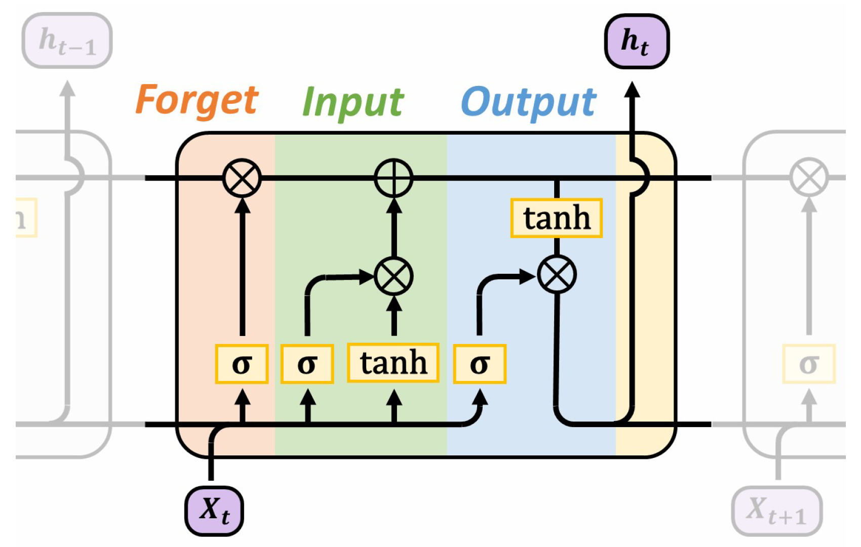
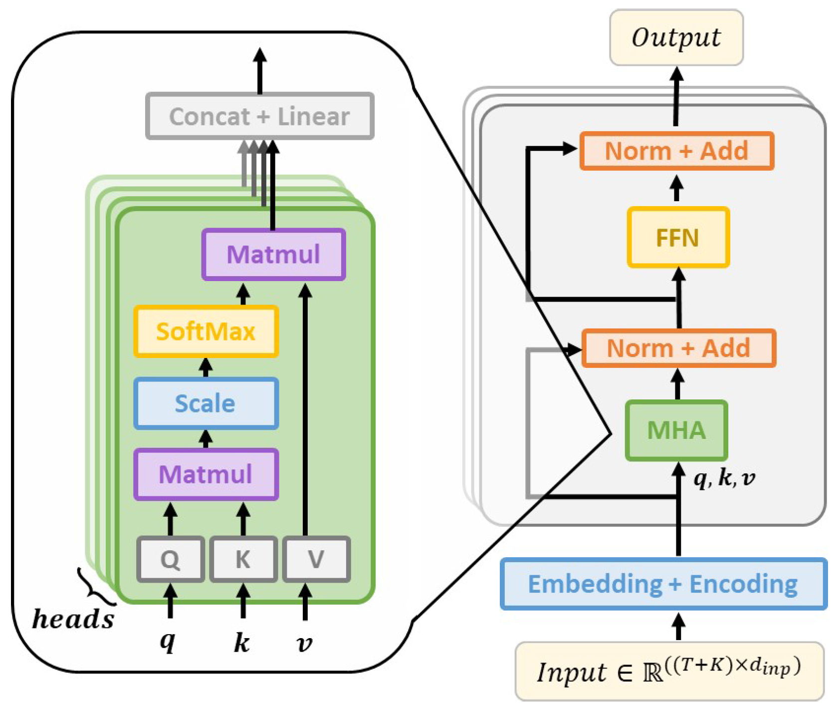
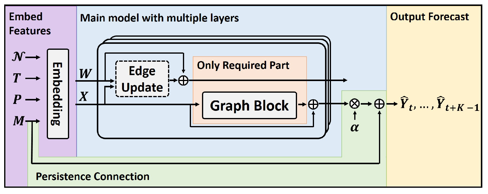
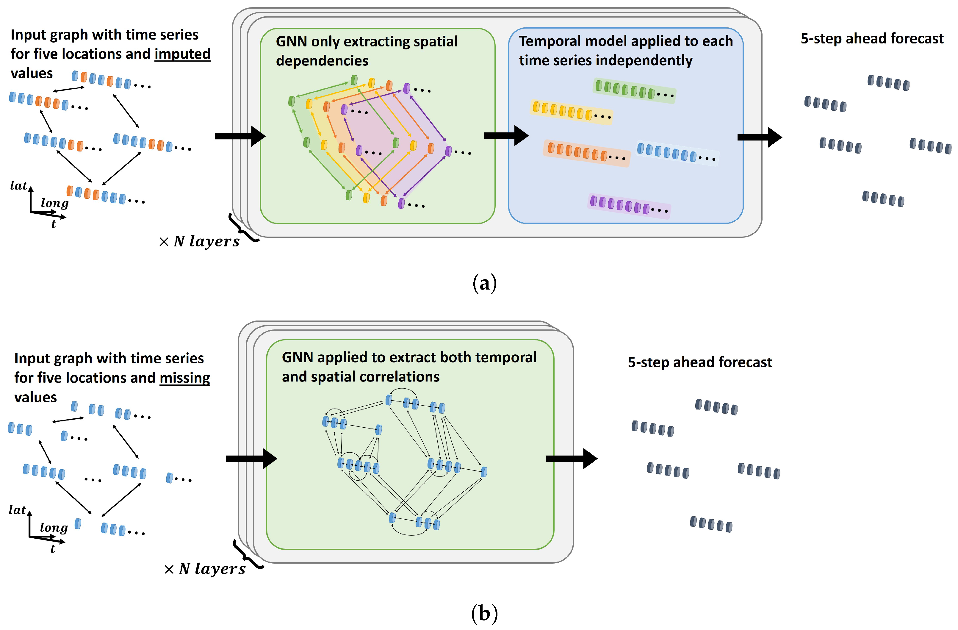
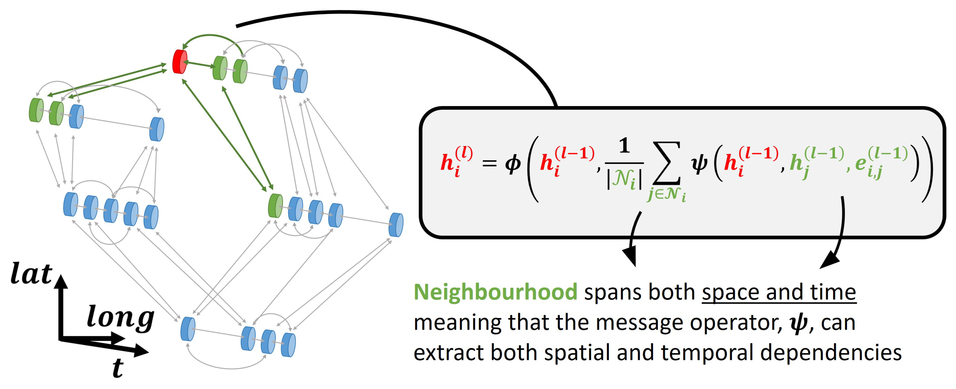
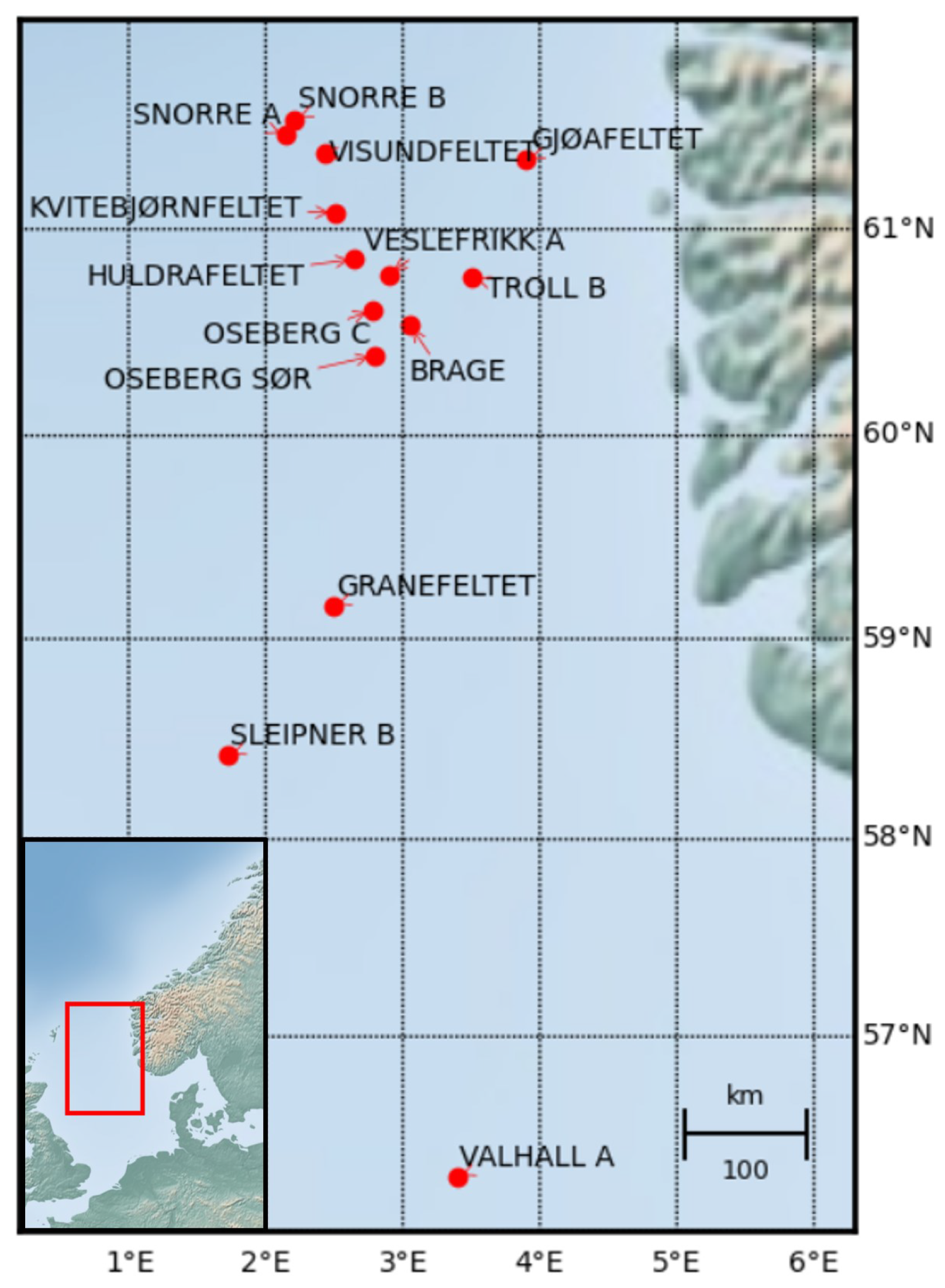
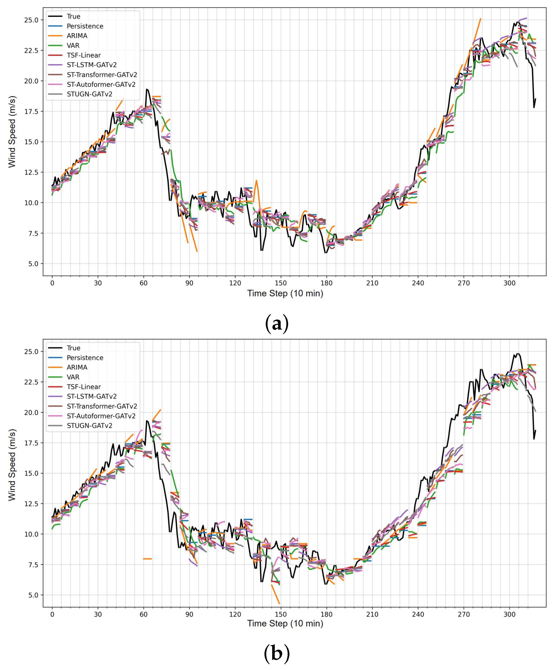
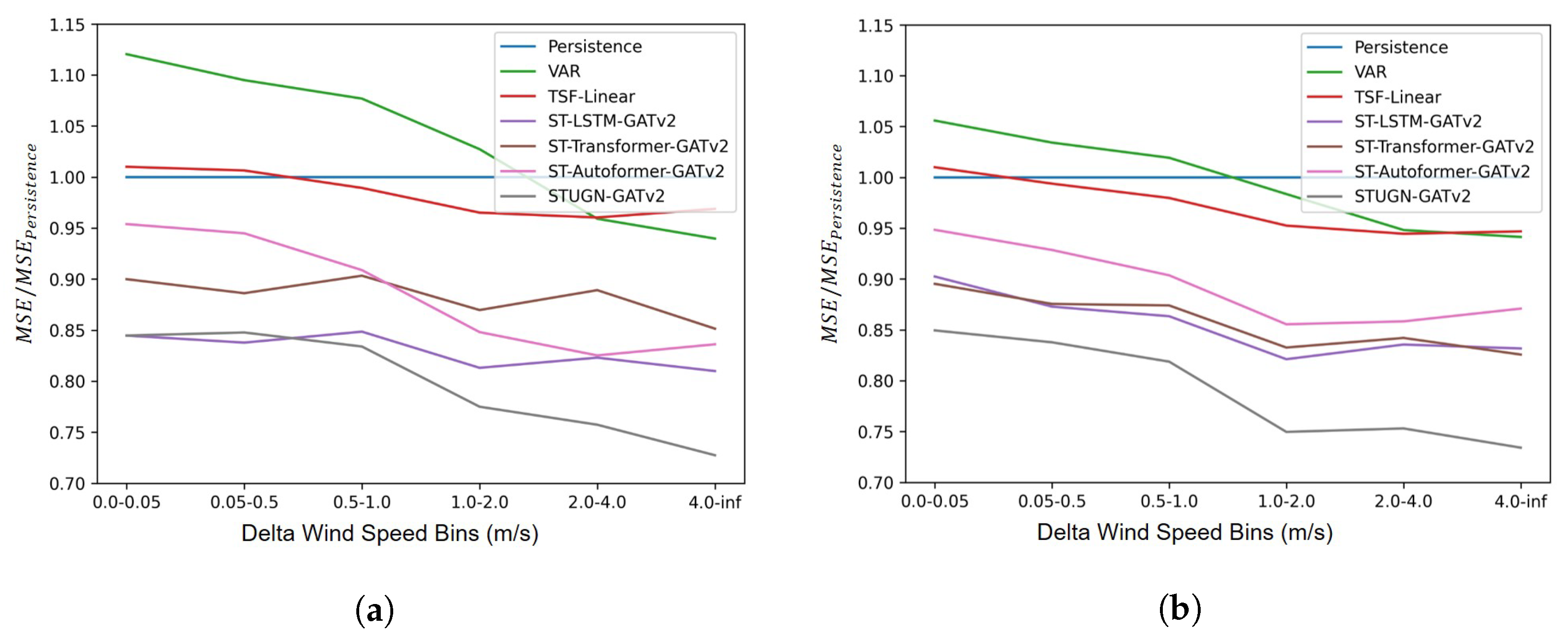
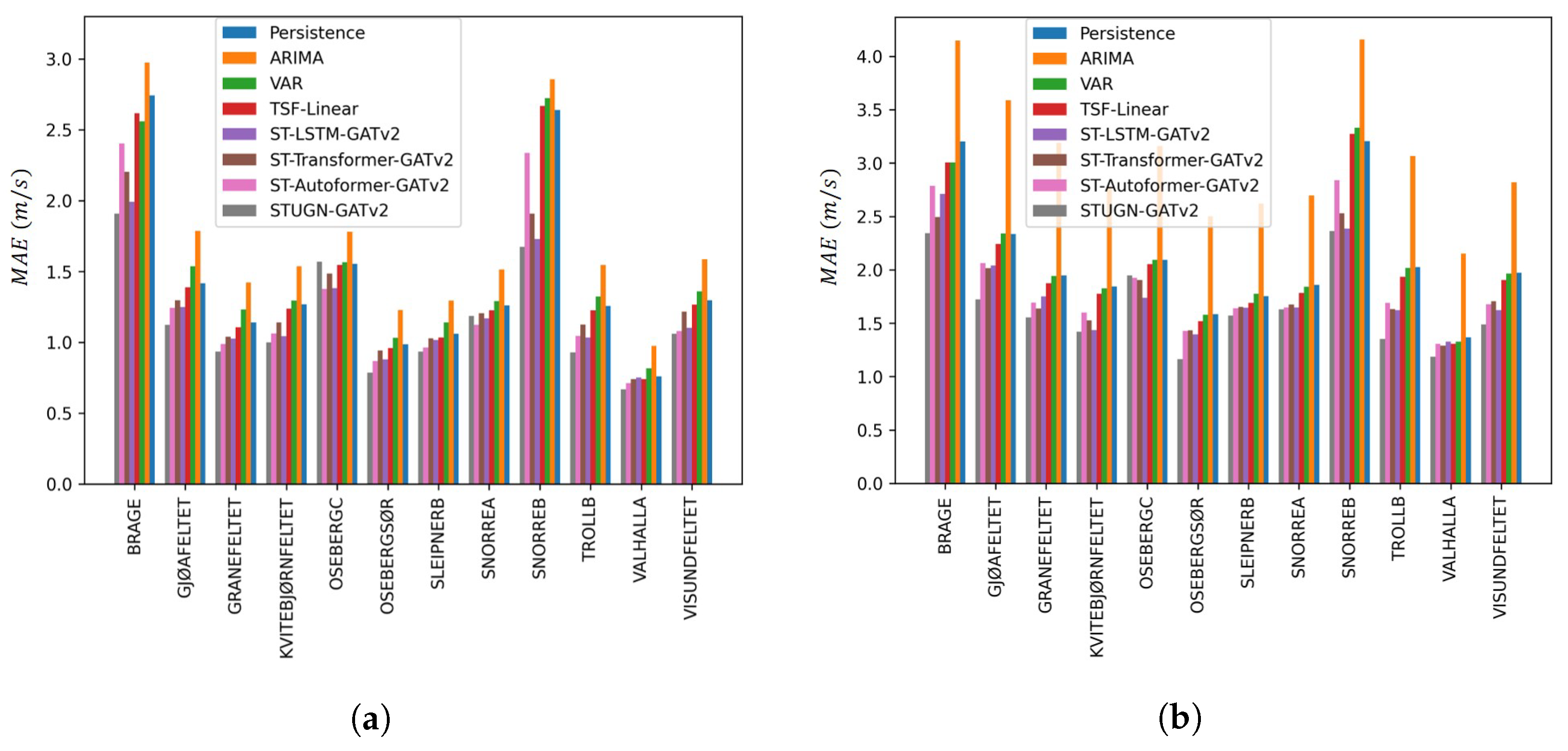
Table 1.
MSEs in m/s for 6-step (1 h)-ahead wind speed forecasts for measurement stations in Figure 6. Values are the mean ± standard deviation from five independent training runs.
Table 1.
MSEs in m/s for 6-step (1 h)-ahead wind speed forecasts for measurement stations in Figure 6. Values are the mean ± standard deviation from five independent training runs.
| Percentage Missing | 0% | 10% | 20% | 30% | 50% | 80% |
|---|---|---|---|---|---|---|
| Persistence | 1.448 ± 0.000 | 1.448 ± 0.000 | 1.455 ± 0.000 | 1.487 ± 0.000 | 1.585 ± 0.000 | 2.098 ± 0.000 |
| ARIMA | 1.707 ± 0.000 | 1.707 ± 0.000 | 1.716 ± 0.000 | 1.740 ± 0.000 | 1.821 ± 0.000 | 3.073 ± 0.000 |
| VAR | 1.488 ± 0.001 | 1.488 ± 0.001 | 1.496 ± 0.001 | 1.518 ± 0.001 | 1.601 ± 0.001 | 2.084 ± 0.001 |
| TSF-Linear | 1.418 ± 0.000 | 1.418 ± 0.001 | 1.424 ± 0.000 | 1.454 ± 0.000 | 1.545 ± 0.001 | 2.029 ± 0.000 |
| ST-LSTM-MPNN | 1.197 ± 0.002 | 1.198 ± 0.002 | 1.206 ± 0.003 | 1.236 ± 0.008 | 1.322 ± 0.006 | 1.773 ± 0.004 |
| ST-LSTM-GATv2 | 1.185 ± 0.010 | 1.187 ± 0.006 | 1.195 ± 0.008 | 1.227 ± 0.009 | 1.310 ± 0.011 | 1.767 ± 0.012 |
| ST-LSTM-TGAT | 1.208 ± 0.007 | 1.207 ± 0.006 | 1.213 ± 0.006 | 1.243 ± 0.009 | 1.327 ± 0.010 | 1.753 ± 0.009 |
| ST-Transformer-MPNN | 1.233 ± 0.012 | 1.233 ± 0.012 | 1.239 ± 0.012 | 1.264 ± 0.007 | 1.344 ± 0.008 | 1.786 ± 0.009 |
| ST-Transformer-GATv2 | 1.268 ± 0.014 | 1.279 ± 0.006 | 1.267 ± 0.022 | 1.305 ± 0.009 | 1.380 ± 0.006 | 1.771 ± 0.017 |
| ST-Transformer-TGAT | 1.283 ± 0.010 | 1.286 ± 0.011 | 1.289 ± 0.005 | 1.319 ± 0.009 | 1.381 ± 0.007 | 1.782 ± 0.006 |
| ST-Autoformer-MPNN | 1.293 ± 0.022 | 1.292 ± 0.012 | 1.292 ± 0.011 | 1.310 ± 0.009 | 1.401 ± 0.008 | 1.866 ± 0.016 |
| ST-Autoformer-GATv2 | 1.273 ± 0.006 | 1.275 ± 0.011 | 1.282 ± 0.005 | 1.313 ± 0.009 | 1.412 ± 0.012 | 1.876 ± 0.019 |
| ST-Autoformer-TGAT | 1.288 ± 0.007 | 1.287 ± 0.008 | 1.294 ± 0.010 | 1.331 ± 0.011 | 1.423 ± 0.004 | 1.891 ± 0.014 |
| STUGN-MPNN | 1.192 ± 0.016 | 1.193 ± 0.014 | 1.201 ± 0.006 | 1.221 ± 0.006 | 1.312 ± 0.019 | 1.668 ± 0.019 |
| STUGN-GATv2 | 1.160 ± 0.015 | 1.160 ± 0.016 | 1.165 ± 0.018 | 1.193 ± 0.013 | 1.277 ± 0.015 | 1.636 ± 0.008 |
| STUGN-TGAT | 1.153 ± 0.010 | 1.155 ± 0.013 | 1.164 ± 0.006 | 1.190 ± 0.011 | 1.264 ± 0.014 | 1.642 ± 0.022 |
Table 2.
MAEs in m/s for 6-step (1 h)-ahead wind speed forecasts for measurement stations in Figure 6. Values are the mean ± standard deviation from five independent training runs.
Table 2.
MAEs in m/s for 6-step (1 h)-ahead wind speed forecasts for measurement stations in Figure 6. Values are the mean ± standard deviation from five independent training runs.
| Percentage Missing | 0% | 10% | 20% | 30% | 50% | 80% |
|---|---|---|---|---|---|---|
| Persistence | 0.810 ± 0.000 | 0.810 ± 0.000 | 0.813 ± 0.000 | 0.823 ± 0.000 | 0.855 ± 0.000 | 0.997 ± 0.000 |
| ARIMA | 0.882 ± 0.000 | 0.882 ± 0.000 | 0.885 ± 0.000 | 0.891 ± 0.000 | 0.915 ± 0.000 | 1.147 ± 0.000 |
| VAR | 0.846 ± 0.000 | 0.846 ± 0.000 | 0.849 ± 0.000 | 0.856 ± 0.000 | 0.882 ± 0.000 | 1.015 ± 0.000 |
| TSF-Linear | 0.803 ± 0.000 | 0.803 ± 0.000 | 0.806 ± 0.000 | 0.817 ± 0.000 | 0.848 ± 0.000 | 0.987 ± 0.000 |
| ST-LSTM-MPNN | 0.749 ± 0.001 | 0.750 ± 0.001 | 0.753 ± 0.001 | 0.764 ± 0.003 | 0.795 ± 0.002 | 0.933 ± 0.001 |
| ST-LSTM-GATv2 | 0.748 ± 0.003 | 0.748 ± 0.003 | 0.751 ± 0.003 | 0.763 ± 0.003 | 0.794 ± 0.004 | 0.931 ± 0.003 |
| ST-LSTM-TGAT | 0.755 ± 0.003 | 0.756 ± 0.003 | 0.758 ± 0.003 | 0.769 ± 0.003 | 0.799 ± 0.002 | 0.928 ± 0.002 |
| ST-Transformer-MPNN | 0.761 ± 0.004 | 0.760 ± 0.004 | 0.762 ± 0.004 | 0.772 ± 0.002 | 0.802 ± 0.002 | 0.937 ± 0.002 |
| ST-Transformer-GATv2 | 0.767 ± 0.003 | 0.770 ± 0.003 | 0.769 ± 0.005 | 0.781 ± 0.002 | 0.809 ± 0.001 | 0.931 ± 0.004 |
| ST-Transformer-TGAT | 0.772 ± 0.003 | 0.773 ± 0.003 | 0.775 ± 0.001 | 0.786 ± 0.003 | 0.810 ± 0.002 | 0.935 ± 0.002 |
| ST-Autoformer-MPNN | 0.776 ± 0.007 | 0.776 ± 0.006 | 0.776 ± 0.002 | 0.784 ± 0.004 | 0.815 ± 0.003 | 0.954 ± 0.006 |
| ST-Autoformer-GATv2 | 0.771 ± 0.003 | 0.772 ± 0.004 | 0.774 ± 0.003 | 0.785 ± 0.004 | 0.820 ± 0.005 | 0.958 ± 0.005 |
| ST-Autoformer-TGAT | 0.775 ± 0.003 | 0.774 ± 0.004 | 0.778 ± 0.003 | 0.791 ± 0.002 | 0.824 ± 0.001 | 0.964 ± 0.004 |
| STUGN-MPNN | 0.748 ± 0.005 | 0.749 ± 0.005 | 0.753 ± 0.002 | 0.760 ± 0.002 | 0.793 ± 0.005 | 0.908 ± 0.005 |
| STUGN-GATv2 | 0.737 ± 0.005 | 0.738 ± 0.005 | 0.740 ± 0.006 | 0.751 ± 0.004 | 0.782 ± 0.004 | 0.898 ± 0.003 |
| STUGN-TGAT | 0.735 ± 0.004 | 0.736 ± 0.004 | 0.740 ± 0.002 | 0.750 ± 0.002 | 0.778 ± 0.003 | 0.901 ± 0.006 |
Table 3.
Estimated energy prediction improvements in kWh for a single 5 MW turbine per forecast horizon of 1 h compared to the Persistence model.
Table 3.
Estimated energy prediction improvements in kWh for a single 5 MW turbine per forecast horizon of 1 h compared to the Persistence model.
| Percentage Missing | 0% | 10% | 20% | 30% | 50% | 80% |
|---|---|---|---|---|---|---|
| Persistence | 0.0 | 0.0 | 0.0 | 0.0 | 0.0 | 0.0 |
| ARIMA | ||||||
| VAR | 0.0 | −0.1 | 0.1 | 0.8 | 1.5 | 2.5 |
| TSF-Linear | 4.1 | 4.1 | 4.1 | 4.3 | 4.9 | 6.4 |
| ST-LSTM-MPNN | 30.0 | 29.6 | 29.9 | 30.9 | 30.6 | 28.4 |
| ST-LSTM-GATv2 | 28.8 | 28.4 | 28.9 | 28.8 | 27.2 | 28.5 |
| ST-LSTM-TGAT | 24.9 | 24.0 | 24.4 | 26.4 | 26.5 | 30.6 |
| ST-Transformer-MPNN | 20.9 | 23.4 | 22.8 | 24.6 | 24.7 | 26.6 |
| ST-Transformer-GATv2 | 19.3 | 18.8 | 20.2 | 20.5 | 22.4 | 29.1 |
| ST-Transformer-TGAT | 18.0 | 17.7 | 18.3 | 19.1 | 20.7 | 29.0 |
| ST-Autoformer-MPNN | 22.3 | 22.5 | 21.3 | 22.2 | 22.5 | 19.3 |
| ST-Autoformer-GATv2 | 21.4 | 20.2 | 21.0 | 21.9 | 21.7 | 21.4 |
| ST-Autoformer-TGAT | 19.8 | 17.8 | 20.2 | 17.8 | 17.5 | 13.9 |
| STUGN-MPNN | 28.5 | 26.8 | 29.0 | 29.8 | 29.9 | 37.8 |
| STUGN-GATv2 | 36.5 | 37.0 | 37.3 | 36.2 | 35.1 | 42.5 |
| STUGN-TGAT | 36.8 | 36.9 | 36.7 | 33.8 | 34.6 | 42.3 |
Disclaimer/Publisher’s Note: The statements, opinions and data contained in all publications are solely those of the individual author(s) and contributor(s) and not of MDPI and/or the editor(s). MDPI and/or the editor(s) disclaim responsibility for any injury to people or property resulting from any ideas, methods, instructions or products referred to in the content. |
© 2023 by the authors. Licensee MDPI, Basel, Switzerland. This article is an open access article distributed under the terms and conditions of the Creative Commons Attribution (CC BY) license (https://creativecommons.org/licenses/by/4.0/).
Share and Cite
MDPI and ACS Style
Bentsen, L.Ø.; Warakagoda, N.D.; Stenbro, R.; Engelstad, P. A Unified Graph Formulation for Spatio-Temporal Wind Forecasting. Energies 2023, 16, 7179. https://doi.org/10.3390/en16207179
AMA Style
Bentsen LØ, Warakagoda ND, Stenbro R, Engelstad P. A Unified Graph Formulation for Spatio-Temporal Wind Forecasting. Energies. 2023; 16(20):7179. https://doi.org/10.3390/en16207179
Chicago/Turabian StyleBentsen, Lars Ødegaard, Narada Dilp Warakagoda, Roy Stenbro, and Paal Engelstad. 2023. "A Unified Graph Formulation for Spatio-Temporal Wind Forecasting" Energies 16, no. 20: 7179. https://doi.org/10.3390/en16207179
Note that from the first issue of 2016, this journal uses article numbers instead of page numbers. See further details here.