1. Introduction
Buildings are a crucial component of the future energy transition, as they account for a significant proportion of worldwide energy use and greenhouse gas emissions [
1]. Over the past decade, there has been a significant rise in energy use within the building sector. Specifically, between 2010 and 2021, energy use in buildings experienced a more than 17% increase, surging from 115 exajoules (EJ) to nearly 135 EJ [
2]. Building efficiency optimization and decarbonization are therefore essential for achieving low-carbon economic goals. In Europe, more than 220 million buildings were built before 2001, making up 85% of the EU’s building stock. Many of these buildings will still be standing in 2050. Many of them are inefficient in terms of energy use, and many rely on fossil fuels for heating and cooling, as well as old appliances and outdated technologies [
3].
The European Commission has set ambitious targets to decarbonize the building sector as part of the European Green Deal and has implemented the Energy Performance of Buildings Directive (EPBD) to promote building energy efficiency and reduce greenhouse gas emissions [
4]. One of the key components of EPBD is the Energy Performance Certificate (EPC), which shows an estimation of a building’s energy efficiency. The EPC has become an important source for energy planning and policymaking in the building stock. From the widely acknowledged importance of the upcoming building renovation wave in Europe [
3] energy analysis for existing buildings has emerged as a powerful input to foster renovation plans. EPC databases have become one of the main sources of building energy information, playing an important role in policy making or urban transition of the building stock. The accuracy of the estimated EPC has, however, been questioned [
5]. Building energy analysis is highly sensitive to the quality of input data and the methodology for the analysis itself. For existing buildings, the minimum required inputs may not be available, and the analysis will inevitably rely on assumptions. To organize the assumptions, a set of boundaries is defined for the energy performance assessor, while keeping the framework open for high applicability, but also prone to subjective evaluations [
6]. As such, the analysis outcomes may not accurately explain the current building energy performance. This can eventually cause inefficient retrofit plans and or unnecessarily expensive and infeasible renovation measures.
Enriching the current EPC calculation methodology with building-monitored data has become essential to identifying energy-saving potential and further improving the building stock energy efficiency [
7]. Disaggregating buildings’ energy consumption by energy services is a valuable approach for understanding and optimizing energy usage in buildings [
8]. End-use disaggregation involves breaking down the total energy consumption of a building into specific categories such as space heating, space cooling, appliances and lighting, water heating, and cooking. Space heating, cooling, domestic hot water, and lighting are the major contributors to energy use in buildings.
The past few years have seen widespread implementation of metering systems at the individual building level. These systems usually record the overall energy performance of a building and therefore, do not give any indication of breakdown in the end-use services. Therefore, techniques to disaggregate end-uses from existing meter infrastructure enable enhanced energy data analytics capabilities. The breakdown of energy consumption in buildings varies depending on factors such as building type, climate, and region [
9,
10,
11,
12,
13].
This research caters to these gaps and provides accurate end-use energy analysis with low-quality and easily accessible inputs. The methodology presents a holistic framework to overcome the different issues by adopting a variety of methods when considering varying data characteristics. The use of load disaggregation techniques to identify the end-use building services based on data availability is investigated. The paper is outlined as follows: The following section discusses the state-of-the-art techniques in end-use load decomposition.
Section 2 introduces the devised data-driven methodology with the explanation of the implemented data-driven load decomposition techniques in addition to introducing different case studies to demonstrate the presented framework.
Section 3 presents the outcomes of the applied methods in demonstration cases.
Section 4 lists the discussion, limitations, and boundaries of this research.
Section 5 concludes the presented study and presents outlooks of the work.
State-of-the-Art Techniques in End-Use Load Decomposition
Although buildings are typically equipped with energy meters that monitor bulk energy consumption, most buildings still lack adequate submetering that can disaggregate energy use into its constituent end-uses and allow operators and energy managers to monitor the flow of energy within a building and help identify anomalous consumption [
14]. This exists mainly due to the lack of sufficient input data [
15]. Building physical characteristics such as heat transfer rates are not always available. Some technical features of the installed HVAC may not be accurately available. The efficiency of the system is mostly overestimated. Often, there is a lack of required domain knowledge to perform an accurate analysis. Energy analysis with insufficient input data requires knowledge of data enhancement methods and experience with energy calculation methodologies. Moreover, there is a lack of accurate methods that are computationally fast [
16].
There are three main methods to disaggregate the end-use in the buildings [
17] namely direct metering using multiple sensors/meters (such as data sets available [
18,
19]), non-intrusive load monitoring (NILM) [
20,
21,
22,
23,
24], and statistical approaches [
18,
25]. While direct metering provides accurate data, installation and maintenance costs are considerably high and not feasible in every residential and commercial building. In contrast, NILM uses less equipment and allows for energy usage monitoring without directly interacting with each device, which makes it convenient and cost-effective. However, NILM requires the installation of advanced sensors for data acquisition, and calibration for signal-device matching, and heavily relies on accurate algorithms for energy allocation. In recent years, NILM approaches have gained momentum as artificial intelligence (AI), embedded devices, and the Internet of Things (IoT) have advanced substantially [
26]. In many applications, such as providing an informative breakdown of the energy use of the house, only a good estimation of the energy use for different appliances will suffice. In this case, theoretical calculations are viable options in comparison to intrusive load monitoring. However, the selection and implementation of the optimal algorithm is often a complex decision, as this requires a deep understanding of the subject matter. This reliance on expert knowledge diminishes the effectiveness of the available input data. Consequently, there is a requirement for a comprehensive framework that can facilitate the development of suitable methodologies for building energy decomposition. Such a framework should accommodate diverse data accessibility and leverage multiple data sources to extract maximum value. Lastly, statistical methods, breakdowns of building energy consumption based on aggregate energy data, and detailed residence descriptions without requiring real-time monitoring are mostly used for national-level analysis [
17]. In most cases, they use either simplified regression models or engineering methods to construct their models (such as [
27]). With smart meters, utilities can retrieve energy measurement data remotely based on fine-grained time intervals [
28]. The data collected from smart meters can be used for various purposes, such as identifying submetering needs, developing an optimal permanent submetering strategy, and conducting a metering assessment to better understand energy use characteristics [
29,
30,
31,
32,
33].
End-use heat disaggregation techniques often differ based on the time resolution considered for the analysis. A study by Bacher et al. used a time series of 10 min values of total heat load for a single-family house [
34]. The authors formulated a non-parametric model to estimate the space heating using the fact that domestic hot water (DHW) appears as short spikes in the time series of the gas consumption, while space heating (SH) has a lower frequency and appears for more hours. Hence, they used a kernel smoother, and all the values significantly above the kernel smoother were considered to be the DHW heat demand spikes.
Marszal-Pomianowska et al. [
7] used a simple methodology, which allows for the calculation of both the mean hourly and daily profiles of DHW heat demand using hourly data from the overall heat demand of the building. This contributes significantly to enhancing our comprehension of DHW usage. The authors validated their study by applying the method to a dataset comprising hourly readings of total heat consumption from 38 single-family houses supplied by district heating.
Neu et al. [
35] modeled five residential archetypes to generate the required operational data with the required frequency. The methodology generates activity-specific occupancy and appliance electricity use profiles using time of use survey (TUS) activity data coupled with Markov Chain Monte Carlo techniques. By combining the probability distributions for TUS activities with the average daily DHW energy demand, depending on the household size, day type, and season, it is expanded to DHW energy demand profiles. On a national level and every 15 min, the simulations provided variations in DHW consumption, heat demand, and energy usage for DHW heating. Typically, a model like this is only appropriate for a specific building. Additionally, practice demonstrates that such models are significantly less precise than analyses based on actual measurements [
35].
Several urban multi-energy simulation models have surfaced in the past few years that deploy data-driven physics-based calculations for end-use heat load estimations. The UK residential building stock model used a resistor-capacitor (RC) model for space heat load estimations and an occupancy model with existing activity profiles to estimate DHW consumption [
36]. While the results provide an acceptable overview of the UK building stock, the model fails to render satisfactory results at the individual building level. Fischer et al. [
37] employed a stochastic bottom-up approach to estimate heat loads for single-family dwellings. In that study, the authors used a behavioral model that required data regarding occupants’ activities. They further used a simplified physical model to estimate a realistic heat load profile, while keeping the modeling tasks and computational efforts manageable.
Data-driven models have also gained significant popularity when segregating and estimating the DHW consumption from the total heat load. Sorensen et al. used the hourly heat consumption values and developed a linear regression model considering outdoor temperature, hour of the day, weekdays, and holidays as the explanatory variables [
38]. Leiria et al. [
14] used the energy monitoring data (1 h resolution) of 28 Danish apartments to demonstrate the disaggregation of SH and DHW demands. The authors compared different techniques for disaggregation looking for the optimal method to estimate the SH and DHW separately. They proposed their method which is a combination of Support Vector Regression (SVR) with the Kalman filter.
The energy signature curve (ESC) technique is a data-driven that exploits statistical models to explain the relationship between the outdoor temperature and the total heating demand [
39]. Building energy signature analysis is a well-established tool for understanding the relationship between building energy use and outdoor temperature and analyzing energy-saving potentials. This approach facilitates the determination of average hourly and daily patterns in DHW (Domestic Hot Water) demand based on hourly data concerning the overall building heat demand. This contributes to a deeper understanding of how DHW is used. We verify the effectiveness of this approach using data collected from both single-family houses and apartments. Subsequently, we apply this approach to a dataset containing hourly readings of total heat consumption from 38 single-family houses connected to district heating.
The process of disaggregation of building demand, as discussed above, has seen the use of different datasets at various time resolutions. The subsequent implementation of disaggregation techniques does not give any consolidated indication of their application in the built environment. As such, this paper aims to provide a holistic view (or a set of guidelines) of end-use load disaggregation under different levels of detail of the building stock data. Furthermore, this study calculates updated building U-values that can be used to further bridge the energy performance gap.
2. Methodology
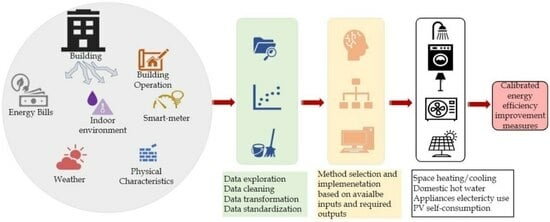
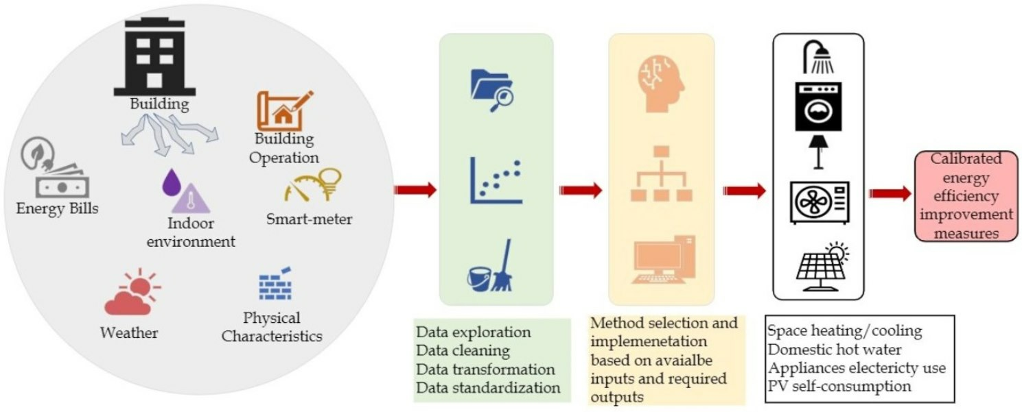
The methodology, proposed in this study, provides a framework to identify building energy end-uses for different buildings. The method has a major focus on the use of energy bills, time-series consumption patterns, indoor environment variables, and building physical parameters (
Figure 1). This framework represents one of the first attempts at establishing guidelines when the data available are either too limited to perform a whole-building energy simulation or the data are not integrated into the standard building energy performance methodology. The techniques represent a simplified approach to bridge the gap and facilitate the adoption of smart meter data in conventional building energy performance calculations.
Data collection is the initial step in the workflow that retrieves the energy bills, end-use consumption statistics, local weather information, indoor operational data, and time-series datasets for buildings under consideration. The availability and the requirement of these dataset differs from one technique to the other. Energy bills and end-use consumption statistics are normally required on an aggregated level. This could range from monthly to yearly aggregates over time. The local weather information is extracted either from the local weather stations or from the typical meteorological weather files. The indoor operational data include mainly the indoor temperature profiles and act as the data enhancement requirements to calibrate the disaggregated end-uses. The time-series datasets mainly focus on total heat consumption values for a fixed time resolution. In the event of the availability of static building data (e.g., U-values), each time series is further linked to building physical parameters.
The second step is data preprocessing when dealing with smart meter time-series data. The data need to be checked for duplicate values, irrelevant timestamps, missing values, and negative measurements. The data preprocessing procedure mainly implements data cleaning and data transformation processes.
Data Cleaning: This is a standardized process to be implemented before any data-driven model formulation. The implementation of data cleaning removes irrelevant data points including missing values, duplicate data, and other inconsistencies that do not align with the existing data patterns.
Data Transformation/Standardization: This process deals with the data structure, data integration, and data normalization. Some of the examples include scaling different variables to a similar range or creating a dataset with standard characteristics (mean = 0 and standard deviation = 1).
The next steps include the selection of an appropriate assessment method and the output estimation step, which are different for different methods and are explained in detail below.
The techniques presented below calculate the end-use services in buildings, which include space heating, domestic hot water, space cooling, ventilation, lighting, and other purposes (e.g., PV self-consumption).
2.1. Calibrated Theoretical Energy Decomposition Technique
This technique is an adaptation of the Measured Energy Performance Indicator (MEPI-) tool resulting out of the X-tendo project [
40] and is applicable to all types of buildings except for industrial buildings. MEPI follows the general principles as described in EN 52000-1 series [
41]. The primary input for the MEPI at the building level comprises measurement data concerning the energy supplied to and discharged from the building unit. These data are categorized by energy carrier and application. MEPI improves the estimated energy performance indicator with measured energy use. The assortment of meters required within the monitoring setup can encompass electricity, gas, oil, and heat meters, or a combination thereof. The quantity, type, and placement of these meters, both primary and secondary, are contingent upon the specific system and the architectural layout of the building. Nonetheless, it was recognized within the X-tendo consortium that the essential monitoring infrastructure is often absent in existing building stock. To address this gap, the calculation tool is supplemented by a report that offers strategies for utilizing actual energy consumption data to depict either a portion or the overall energy performance. This approach proves beneficial in scenarios where there is a scarcity of information or in instances involving intricate structures such as malls or hospitals, where employing a purely theoretical methodology would be excessively time-consuming and expensive. The gap between theoretical calculations and actual energy consumption can lead sub-optimal retrofit recommendations [
40].
The proposed enhancement improves the quality of MEPI energy analysis by using measured indoor temperature. As such, the technique initially estimates the theoretical energy use for different services using EN 52000-1 series [
41], and then the estimated theoretical values are calibrated using energy bills. In the final step, calibrated estimated energy uses are corrected by indoor temperature. Three steps are followed to derive the calibration factor for the estimation of calibrated energy use:
Step 1 is for the estimation of theoretical energy use (Equation (1)) that is decomposed into different services by different energy carriers where available. Energy carriers are electricity, district heating, district cooling, biofuel, oil, and gas.
where t stands for theoretical, E
i,t is theoretically calculated per energy carrier i for different energy services namely space heating, domestic hot water, space cooling (if applicable), ventilation, lighting, and other services wherever applicable:
Etotal,i,t is total theoretical energy use by energy carrier i (kWh) which is a summation of space heating, domestic hot water, space cooling, ventilation and lighting electricity consumption, and energy needs for other services if applicable.
Step 2 involves the calculation of calibration factors. Equation (2) is used at this step.
where E
s,i,t refers to the theoretical energy demand for services (as listed previously) for energy carrier i. Calibration factor f
s,i is accordingly calculated for service s (the same services as listed above) for energy carrier i. f
s,i shows the share of the energy service s from the total energy use.
Step 3 assigns actual energy use based on calibration factors according to the equation below.
Es,i,c stands for calibrated energy use for service s including space heating, domestic hot water, space cooling, ventilation and lighting electricity consumption, and other services if applicable for energy carrier i. The main underlying assumption for this method is that the theoretical decomposition and actual decomposition follow similar shares of different services. Hence, the absolute calibrated value of different services can derived using the fs,i estimated from the theoretically estimated energy decomposition. Etotal,i,a refers to actual energy consumption derived from measurement for the period of the analysis.
The calibration factor is calculated for the period when the measured energy use is available. Moreover, the frequency of the calibration factor corresponds to the frequency of the measurement. For example, if the energy is measured via annual energy bills, the calibration factor is an annual factor.
This method helps identify energy use of certain specific services more accurately, yet in some cases, these results might be largely biased by the unoccupied period or seasonal variations in energy use patterns. Thus, it is sensible to use the average monthly consumption measured for several months or implement calibration factors for multiple months to reduce the possible error margins. In this case, each month has a different calibration factor that is applied to the theoretical energy decomposition.
To improve estimated energy use for end uses, heating degree days (HDD) and cooling degree days (CDD) are estimated using measured indoor and outdoor temperatures with high frequency. While, in the MEPI tool, national or regional standardized values for indoor and outdoor temperatures are used to define HDD and CDD. An assumption is made for the outdoor temperature after which the heating load is considered zero. Similarly, an assumption is made for the temperature before which the cooling equals zero. We assume a daily average outdoor temperature of 15 °C after which heating is not activated. If the indoor temperature is not available, the devised heating setpoint can be assumed as the average indoor temperature to perform the analysis.
The daily average of DHW is corrected for the number of occupants for the measurement period. The corrected daily average value is then extrapolated to the full year according to the number of days. The standard values for DHW consumption per person for different buildings are found in table G.12 from ISO 13790 [
42]. The system energy efficiency, if known, is applied to calculate DHW energy demand. If efficiency is not known, the measured energy delivered for domestic hot water in the specific period of the measurement is directly used after corrected according to the actual occupancy rate.
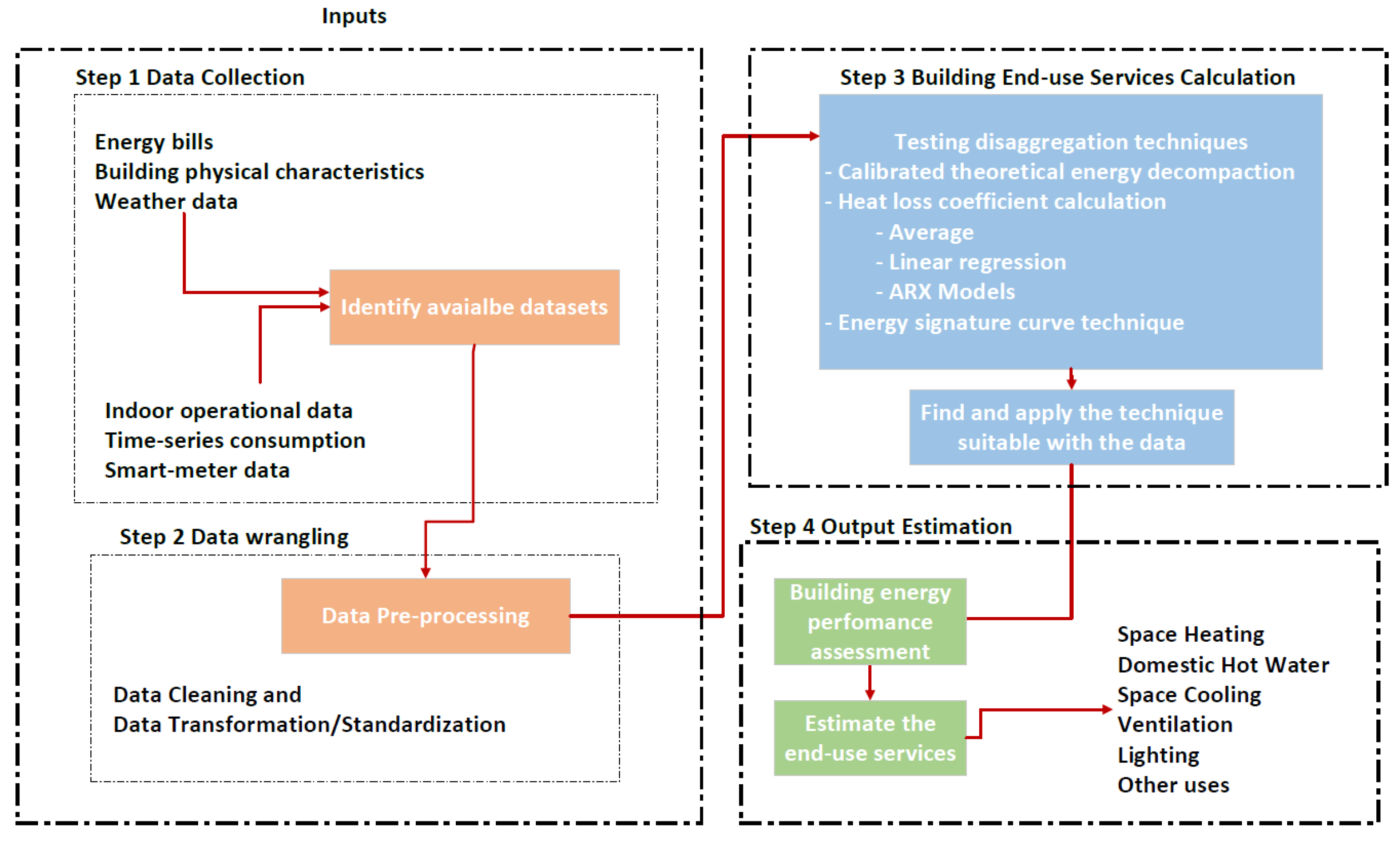
To make use of input data with measurement periods of less than a year, the self-consumption is derived in the presented method based on the actual hourly measurement of the PV generation of a certain period and then is extrapolated linearly. The full-year PV generation is then calibrated by means of solar radiation hourly profile from a standard year derived from PVGIS [
43]. The proposed correction includes the steps shown in a high-level flowchart in
Figure 2.
2.2. Heat Loss Coefficient (HLC) Calculation Technique
On-board monitoring (OBM) can largely improve the accuracy of energy performance analysis [
44]. Specifically, OBM can explain energy performance of a building as built, while theoretical estimation based on building physical parameters can contain disinformation about the current situation of a building. The HLC, which can be identified using OBM data, describes the insulation quality and airtightness of a building envelope in a single factor which makes it an understandable method in application and simultaneously highly explainable in the results [
45]. HLC can be a noninvasive method that can be applied remotely. This can decrease the energy audit costs significantly and introduce these methods as viable options for upscaled energy performance analysis. Additionally, indoor temperature and sub-hourly energy use from smart meters are recently becoming more accessible. However, OBM data are also strongly influenced by occupant behavior, such as heating and cooling behavior and domestic hot water use. Therefore, applying energy decomposition methods correctly before defining the HLC is crucial. Moreover, energy analysis based on OBM is a general term that does not specify which parameters are measured and how they can improve the analysis. Energy use of certain appliances could be directly measured, e.g., sub-metering of electricity use, and water flow meters that measure domestic hot water.
The proposed HLC technique in this study derives the theoretical energy uses for various services as presented previously in the above section as a calibrated theoretical energy decomposition method. The HLC is then calculated using the available measurements for energy use and indoor temperature. Depending on the available data (number of parameters, time step, and data set length), three different models are used to identify the HLC, namely, the average method, linear regression models, and ARX models [
44]. The average method and linear regression models are static methods that disregard any dynamic building phenomena, while the ARX model is a semi-static method that considers dynamic phenomena by integrating data from previous time steps. The HLC methods below are applicable to OBM data collected during the heating season, i.e., there is energy use for space heating and not for cooling.
2.2.1. Average Method
The average method is described in ISO 9869-1:2014 [
27]. This method requires a preliminary step that is to prepare the inputs, which are the different heat loss/gains of the building. To feed the average method with disaggregated energy use, of the building, the calibrated theoretical energy decomposition technique, explained in the previous section, is used. The average method assumes that the division of the mean heat flow rate by the mean internal-external temperature difference is equal to the HLC when a sufficiently long period (here shown as time steps between j and n) is considered:
where:
QSH,j is heating power (W) for space heating in time step j, accounting for heating demand caused by transmission, ventilation, and infiltration heat losses. Transmission heat losses should be considered toward the ground, the exterior, adjacent unconditioned zones (e.g., garage, attic, cellar …), and adjacent heated zones (e.g., neighbors). If measured QSH is not available, the calibrated energy decomposition method explained in the previous section can be used to estimate this parameter.
Qint,j is internal heat gains (W) for time step j from appliances and metabolic heat gains (MHG). MHGs are often disregarded in residential buildings.
Qsol is the solar heat gains in W for time step j.
Qvent is ventilation system heat losses in W for time step j.
Qtot is total heat loss as a summation of the listed heat losses for time step j.
Ti,j is the average indoor temperature of all rooms (K) for time step j.
Te,j is the outdoor temperature (K) for time step j.
2.2.2. Linear Regression Models
Using regression models to explain a correlation between the parameters of a system is a general data-driven approach that can be adopted for HLC estimation [
46]. In all the LR models, HLC is the coefficient of the independent variables such as indoor temperature, and the statistical model is fit to predict the dependent variable such as energy use. Depending on the available dataset, different types of linear regression models are formulated to estimate the heat loss coefficient (HLC). More available parameters as input data serve as more independent parameters in the LR model that can be used to better predict the dependent parameter. All the models are formulated according to some physical assumptions as will be elaborated below. In general, and as a trade-off, linear regression models disregard part of the system interactions to gain simplicity. This study devises three linear regression models (LR1 to LR3) as presented below.
LR1 is used when the measured indoor and exterior temperatures are accessible while solar radiation and internal gains are not known and thus are not incorporated. Note that this method is naturally not recommended for buildings with high internal and solar gains (e.g., an office building in Southern Europe). In LR1, HLC is derived using linear regression models that can explain the relation below.
LR2 additionally incorporates internal gains and hence is more reliable for case studies with high internal gains.
LR3 enhances the method LR2 with the consideration of solar heat gains inside the building.
where gA is solar aperture (m
2) and I
sol is measured global horizontal irradiation on site in W/m
2. To derive the HLC using Equation (7), the linear model is regressed over indoor and outdoor temperatures in addition to solar gains in the proposed equation. HLC is estimated so that the squared differences between true data and predicted data are minimized.
Each of the models incorporates and disregards different terms, which can result in a slightly different estimated HLC. Generally, it can be expected that the reliability of the model increases with the number of considered parameters.
Linear regression models are static models that can only be applied on daily averaged data, or even weekly or monthly data. Therefore, dynamic aspects such as indoor and outdoor temperature fluctuations and the impact of the thermal capacity of the building are not considered in the calculation procedure. Additionally, linear regression models are less robust due to a lower confidence interval in parameter estimation [
46]. To include the dynamic phenomena, auto-regressive models with exogenous inputs (ARX-models) are applied to data with a shorter time step.
2.2.3. ARX Models
Autoregressive exogenous input (ARX) models [
44] are a type of statistical model that represents a time series as a linear combination of its past values and a stochastic process considering a set of exogenous input variables. The ARX model is formulated similarly to the linear regression models while backshift operators are applied to the inputs and output of the model. Each of these operators is polynomials of a different order [
47].
where:
ωx (B) is the backshift operator applied to input or output x. Note that the backshift operator is used to detect the correlation between dependent and independent time series even with lags. As such, backshift does not impact the model coefficients, rather it shifts the input to correlate to the outputs with current coefficients. In the case of building heat load, outdoor temperature, and indoor temperature, there is a lag between the time series of these parameters and hence using a backshift operator helps find the correlation. Ti is the average indoor temperature of all rooms (the unit is K). QSH represents energy demand for space heating caused by transmission, ventilation, and infiltration heat losses. Transmission heat losses should be considered toward the ground, the exterior, adjacent unconditioned zones (e.g., garage, attic, cellar), and adjacent heated zones (e.g., neighbors). Qint is internal heat gains (W) from appliances and metabolic heat gains, which are often disregarded. εj is the residual error to be minimized.
For the ARX model, the heat losses are defined using the Lagrange weighting, which is a linear minimum variance weighting between He and Hi:
where:
ωi (1) is the backshift operator of the first order applied to the indoor temperature.
ωe (1) is the backshift operator of the first order applied to the exterior temperature.
ωh (1) is the backshift operator of the first order applied to the heating power.
Time series of different frequency can be used as input for this model. For the selection of an appropriate sampling time interval for the ARX model, a comparison is made among different time intervals using metrics such as the Akaike Information Criterion (AIC-value), R-squared value, and residual magnitudes. The procedure adheres to the Annex 58 report [
48]. If the original sampling time does not yield statistically acceptable results, resampling the time series to longer intervals is proceeded. Finally, the extent to which the dynamics of the time series are incorporated into the estimated HLC will depend on the required resampling period. If an hourly time series is smoothed out to a 12-hourly time series, part of the information and hence the dynamics of the system is lost. As such, the trade-off between the resampling period and the usefulness of the model is a manual task.
2.3. Energy Signature Curve (ESC) Technique
The ESC method is a specific case of linear regression models that assumes that the correlation between the outdoor and indoor temperature of the building mainly relates to the space heat demand due to the presence of seasonal variations [
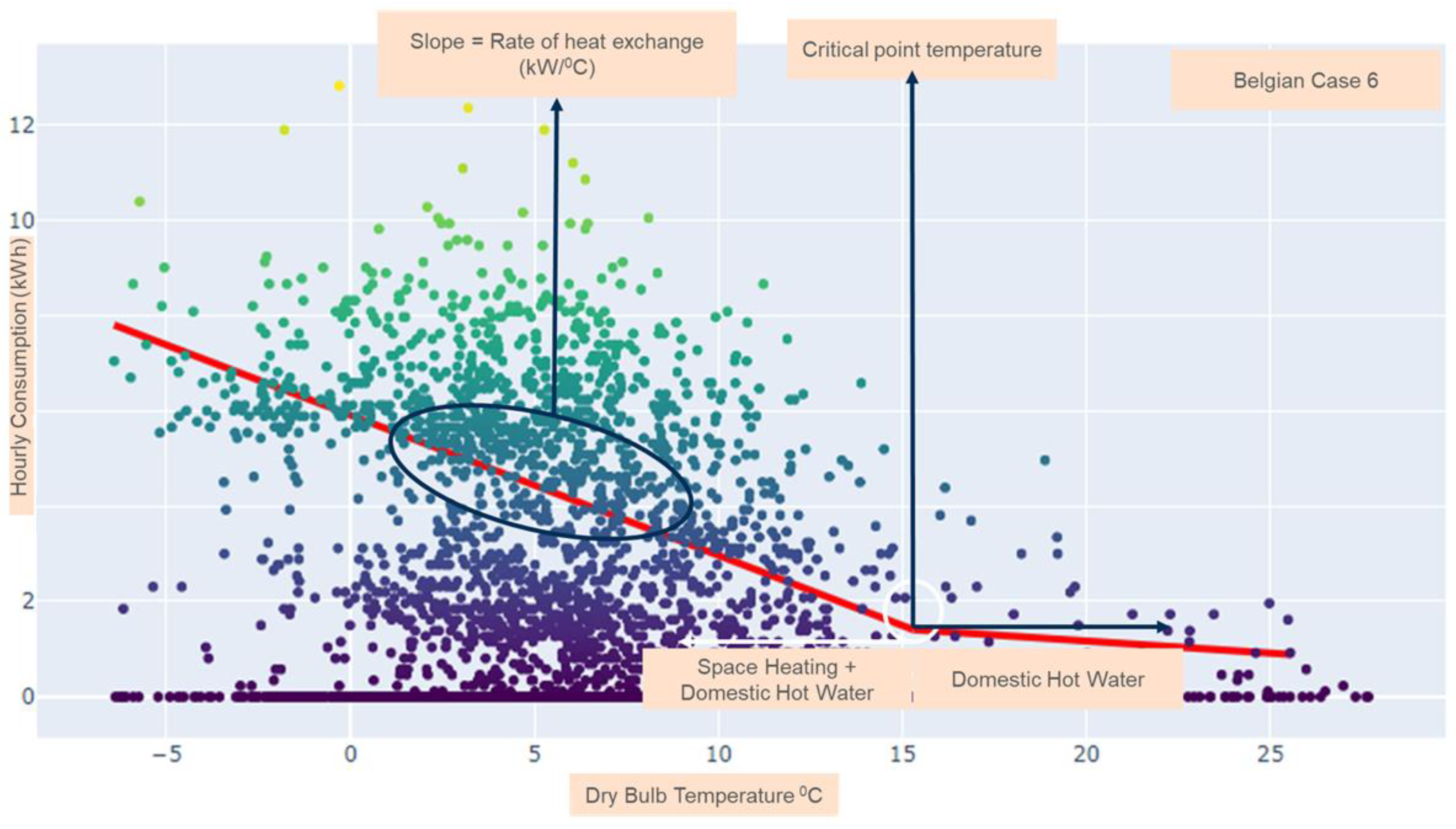
49]. The ESC demonstrates a generalized process workflow for heat load disaggregation using time-series data. A preliminary analysis of the smart meter consumption and weather data indicates that there exists a negative correlation between the outdoor dry-bulb temperature and total heat demand for the households considered. The technique implemented in this research defines a change-point piecewise regression model to disaggregate SH load from the total heat load. It is assumed that the SH load becomes zero below this change-point value (change-point temperature) as with higher temperatures the heating is switched off in a household. Furthermore, the DHW load does not have a significant correlation with the outside dry-bulb temperature at low time resolutions. The assumptions considered to implement this technique are listed below.
The households do not have any cooling loads.
SH only operates before the change point (or at low outside dry-bulb temperatures).
SH load is significantly higher than the DHW load before the change point.
Sleeping period is assumed from 00:00 till 6:00 h.
The energy signature comprises two parts for a household with only heating loads distinguished by the change point value of the independent variable, which in this case is the outdoor temperature. The change point temperature (or CPT) defines the boundary between the use of SH and DHW. The piecewise regression method formulates separate models for these two parts and identifies the value of CPT.
where Q
TH is the total heat demand including space heating and domestic hot water in this scenario.
where Q
TH in the ESC model is the total heat demand in kW. The constants a
0, a
1, and a
2 represent the coefficients of the piecewise model. T represents the outdoor dry bulb temperature and CPT represents the change (or critical) point temperature in °C. ϵ represents the residual error. In principle, a
1 corresponds to the HLC of the building. To derive the coefficients a
0, a
1, and a
2, the time series of outdoor temperature are given as independent variables to find appropriate CPT and model coefficients to predict total heat demand with minimum residuals.
It is worthwhile to mention that the devised regression models are shifted relative to the SH load by a fixed value as the total heat use also includes the DHW load. This fixed value is estimated when the SH is in use before the change point temperature. This fixed value corresponds to the minimum value recorded when the temperatures are below the change point temperature.
DHW heat use is estimated using the residuals calculated by subtracting the total heat load from the modeled SH load. DHW circulation losses are estimated using the average heat load at nighttime. It is also ensured that the values of SH and DHW are positive at any instant in time.
2.4. Case Studies
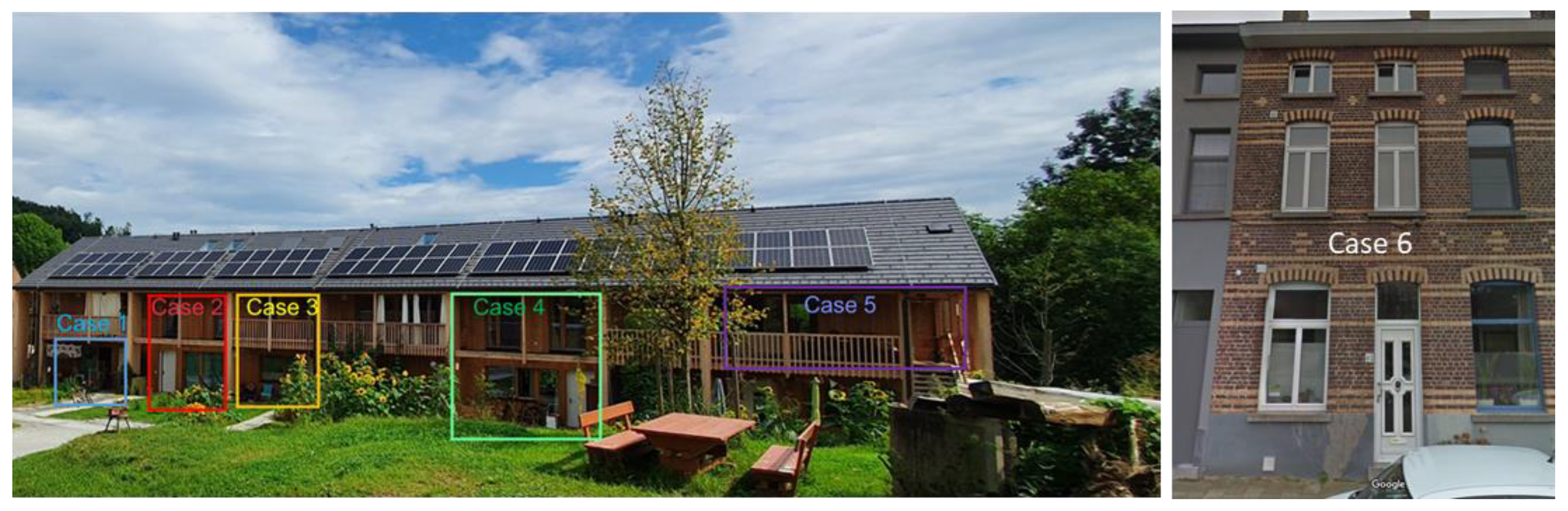
Six case studies have been chosen to demonstrate the calibrated theoretical energy decomposition method and HLC methods. A terraced house in Belgium and five units in a multi-family building in Austria as shown in
Figure 3. These units have sufficient measurements in addition to enough information about their envelope key characteristics (
Table 1) to facilitate a comparison between different methods. The Belgian case study consists of a typical residential house with a condensing gas boiler and radiators for heating. It has neither mechanical ventilation nor an active cooling system. The Austrian cases have shared solar panels and a collective heating system with a biomass boiler. Hourly data for electricity and DHW consumption for these cases are available from October until January for cases 1 to 5 and from August until April for case 6. Moreover, indoor and outdoor temperatures were sub-hourly monitored for all the cases. A significant difference between the average indoor temperature of case 6 with other case studies must be noted.
Table 2 provides a comparison of average monitored parameters across various cases, aiming to highlight the distinctions between the case studies based on measurements.
Theoretical HLC is calculated using infiltration heat loss (natural ventilation is adopted for all case studies) and total transmission heat losses from different heat loss areas as listed in
Table 1.
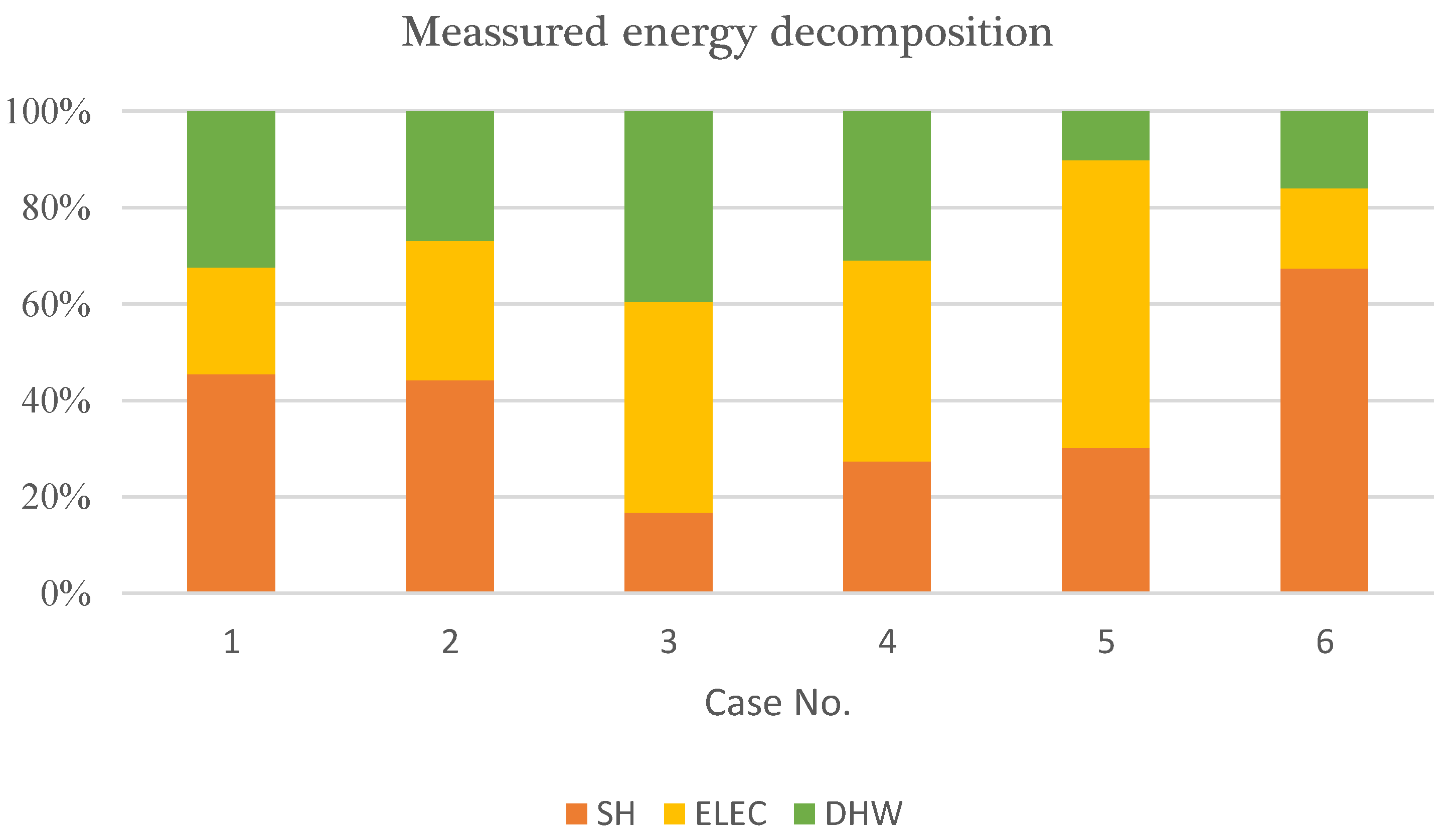
Figure 4 shows the energy decomposition for the six case studies for the measurement period. Different patterns are observed in the different case studies which can stem from different parameters. First, occupant behavior is the decisive factor in the difference between cases 1 to 5 because these cases have similar building physical parameters. Then, the primary distinction between case 6 and other cases lies in the essential difference between the fabrics of case number 6 compared to those in all other cases. Finally, geometrical parameters such as the number of surfaces exposed to the outdoors can impact the decomposition.
The dataset used to demonstrate the ESC method comprises a total of 165 single-family households spread across the Flemish region in Belgium (the meta-data of individual case studies are not published due to data privacy). Each household has a dongle set up by the distribution operator to collect time-series electricity and total gas consumption (SH and DHW) data on a 15 min basis. The data have been originally collected to accelerate the current renovation drive and to identify new opportunities to use time-series information in the current planning and design phase of energy-efficiency measures. The heat for SH and DHW is produced at the individual building level with the measuring equipment recording the total gas consumption use. The data are collected for one year of building operation. The analysis is applied with measured temperature from the Sint-Katerijne district in Belgium, which is within a maximum distance of approximately 50 km of all the case studies.
3. Results
The methodology section presented a variety of methods for building energy disaggregation using monitored data on different levels of accessibility and frequency. It was mentioned that the monitored data can significantly differ depending on the case study, application, and limitations in measurement devices, time, and costs. Moreover, granting access to a building for installing measurement tools can be a barrier in many cases. Therefore, various techniques have been suggested to assist energy assessors in addressing issues with input data. This section demonstrates the application of different methods presented in the methodology section and provides insights into the results derived from these methods.
3.1. Calibrated Theoretical Energy Decomposition
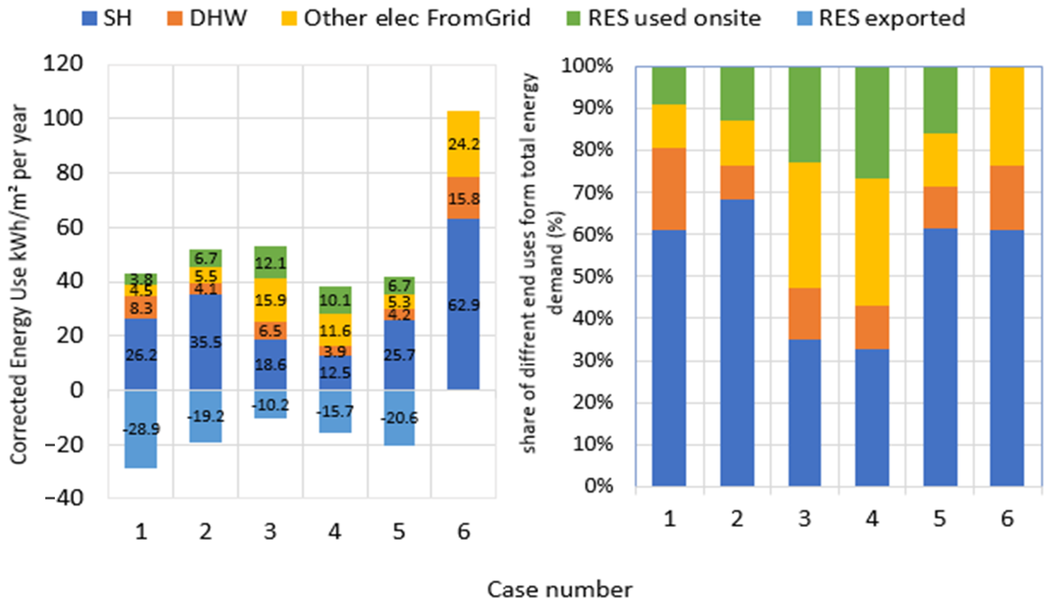
Figure 5 reveals the importance of a case-specific energy decomposition. Although cases 1 to 5 which are different units in one building have similar total energy demand, they have significantly different end-uses. Cases 3 and 4 have less space heating as expected from their smaller heat loss area (
Table 1). Cases 1, 2, and 3 have the same number of solar panels while their self-consumption and exported electricity are not observed similarly. As a result, they cannot expect the same financial return on the same solar panels, regardless of their similarities.
The results reflect the energy decomposition that has been influenced by different factors. This is due to the incorporation of three important elements of this proposed method: (1) applying energy bills, (2) correcting the DHW energy use with the number of occupants, and (3) using indoor temperature for HDD and CDD. A comparison between
Figure 4 and
Figure 5 shows that the energy decomposition use for shorter periods can be reflected on an annual basis. However, the minimum measurement period in this study is 2 months of a heating period. If the building is cooling-dominated or has significant cooling, the observations of this study cannot hold true.
3.2. HLC Technique
This section demonstrates the application of the presented HLC technique using the previous case studies. The availability of sufficient data allows for a comprehensive comparison between the strengths and weaknesses of different methods. As the first step, the outcomes of the calibrated theoretical energy decomposition method, derived and reported in the previous step, are used for HLC estimation. These outcomes can feed different HLC methods depending on the required input for each method as explained in the methodology section.
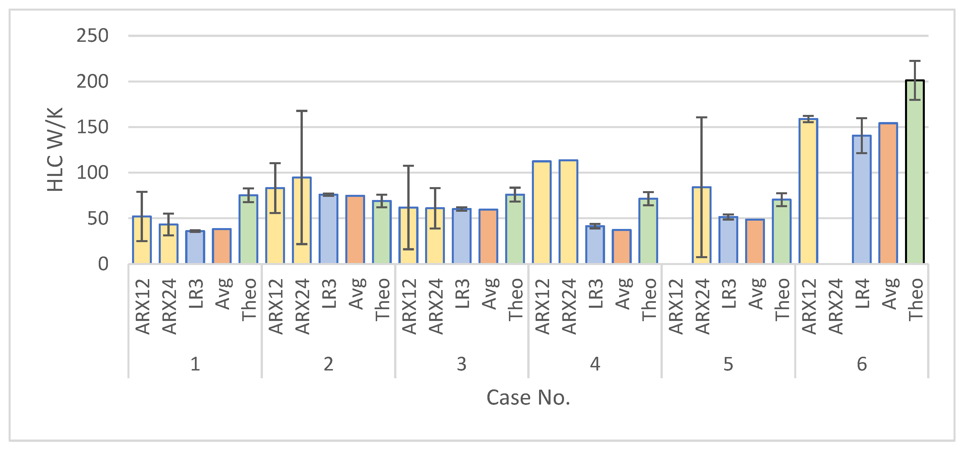
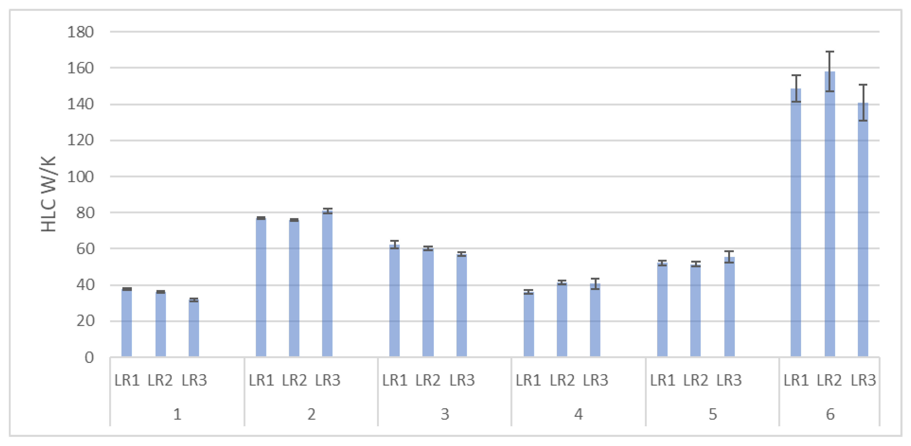
Figure 6 shows estimated HLC with different methods presented in this paper applied to demonstration cases of this study. It summarizes the theoretical HLC as calculated in
Table 1 and the HLC derived from OBM data using the average method (Avg), linear regression methods, and the ARX model for 12 hourly (ARX12) and 24 hourly (ARX24) aggregated OBM data. A comparison between different LR models showed minor differences between LR models and hence only one LR is reported in
Figure 6. The comparisons between different LR models are presented in
Appendix B.
Comparison between the outcomes of different LR models and ARX models shows higher stability in LR models in the results (smaller confidence intervals). The challenges of selecting a reliable ARX model, affected by factors such as model order, data sample time, and parameters make the ARX model complex and prone to cumbersome tuning tasks. ARX models have larger confidence intervals but can significantly alter the identified HLC. Time series data with different sampling times can be used for ARX models. As such, the first question is what frequency results in acceptable outcomes. From
Figure 6, ARX with 24 h periodicity can result in low confidence in the outcomes. While a 12 h periodicity can achieve higher stability and a lower uncertainty. Linear regression provides more reliability checks and can incorporate multiple parameters if available. Choosing the right LR model is a question that is answered according to the available input data. LR models showed high stability in the outcomes with low confidence intervals. As reported in
Appendix A, sampling time has an insignificant impact on the results of LR models.
Differences between theoretical and in situ HLC arise due to different factors such as deviation between predicted and actual user behavior, weather conditions, building materials, and energy decomposition. Note that in situ HLC is not only a physical parameter of the building. It indirectly reflects all the parameters related to occupant behavior, control, and errors in measurements. In situ HLC is also corresponding to the specific year that measurements have been conducted. As such, the number reported for each year can be different. Hence, this method is not recommended for standardized approaches in which buildings within a region are compared with a uniform method considering similar weather.
Moreover, theoretical HLC clearly comes higher than all other estimated HLCs which have been derived from monitored parameters. This is in line with previous reports about the overestimation of building energy demand in comparison to actual building energy demand [
40].
3.3. ESC Technique
For this study, the acquired datasets require a significant amount of data preprocessing. For instance, all the readings were recorded twice for each time stamp. The data also had future time stamps dating to 2065 indicating the outliers in the recorded data. This step removes such instances and refines the dataset for further analysis.
Figure 7 visualizes the relationship between outdoor temperature and hourly gas consumption for the case study in Belgium as explained in
Table 1. Piecewise linear regression is applied to estimate the change point temperature (CPT). The estimated CPT is 15.1 °C, which signifies that there is no requirement of SH above this value. Henceforth, gas consumption mainly relates to DHW consumption above this outdoor temperature. It is worthwhile to mention that this analysis makes it easier to identify CPT using graphical visualization. When analyzing the summer months, mainly the month of July, it is seen that even though the temperature might fall below CPT at certain times during the night, the gas consumption remains zero as the building insulation retains the heat at night. It observed that the consumption can be very scattered, making it difficult to relate outdoor temperature and energy consumption visually. However, the automated procedure of piecewise linear regression intuitively proposes 15.1 °C as the critical point temperature.
The estimated slope of the regression line represents the calculated HLC with the ESC method. This value, 229 W/K as reported in
Figure 7, is comparable with the previously reported HLC for case 6 in
Figure 6. It is observed that the estimated HLC with the ESC method is larger than all other methods. This can be related to the fact that part of the DHW is counted as heating demand. However, the difference with the theoretical HLC value, which is calculated with abundant physical data from the building, is less than 14%. This certifies a promising accuracy for the presented method. A critical observation is that the HKC estimated by ESC is higher than the theoretical HLC. This contradicts the other observations whereas the estimated HLC using measurements was lower than the theoretical HLC.
Energy decomposition based on the CPT is derived for this case study. This verifies that the algorithm can find reasonable outcomes, although it is visually far-reaching. In other words, this method can be a reliable data-driven method for remote energy performance analysis. This theory is confirmed by a comparison between the outcomes from 165 demonstration cases in this study. As mentioned in the methodology section, the slope of the line below CPT corresponds to the building HLC.
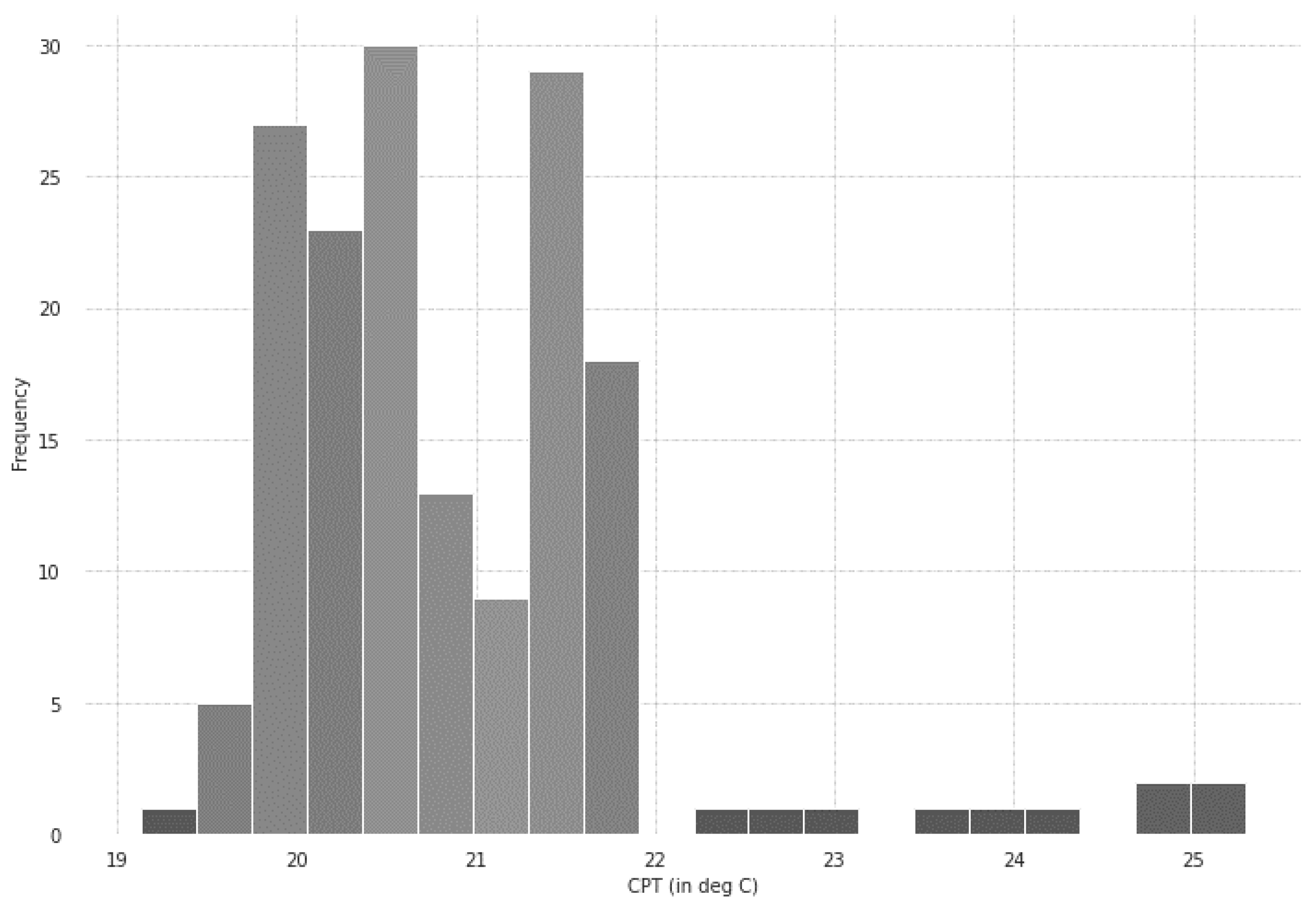
Figure 8 shows the distribution of estimated CPT in all 165 case studies. It is observed that the value ranges between 22 °C and 19 °C mainly. However, few buildings experiment with high CPT, which can stem from multiple reasons such as user behavior and building design in addition to building physical parameters. On the other hand, the physical interpretation of the CPT does not match with the statistically derived value from ESC. As such,
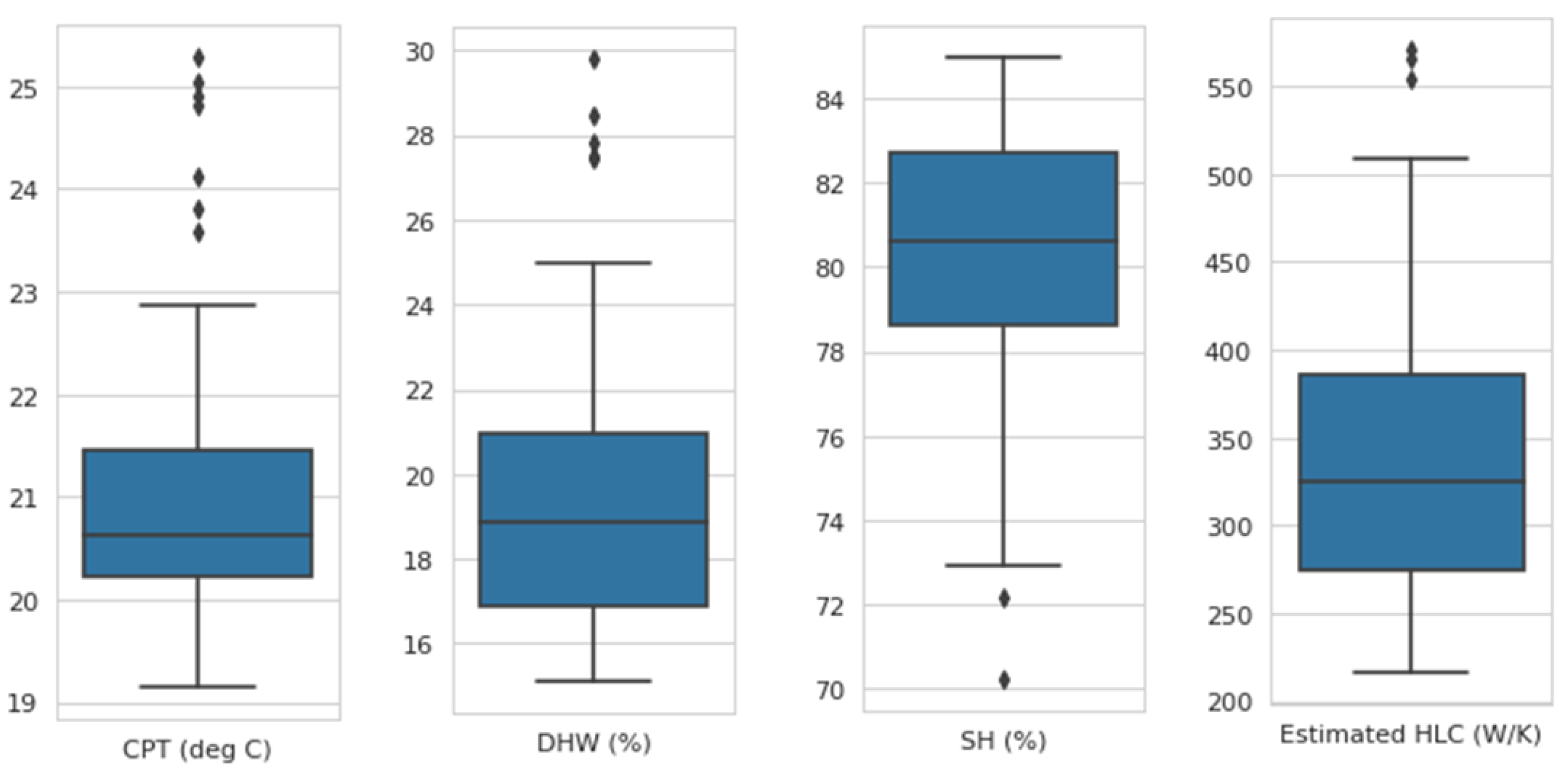
Figure 9 depicts a comparison between different outcomes of the analysis to shed light on the meaning of the statistical parameter CPT. It is observed that the HLC can provide a reasonable range of DHW and SH decomposition. Nonrealistic values for the outliers are not observed. As such, ESC must be adopted for energy decomposition carefully. It cannot give an indication of a physical CPT, while it provides reasonable energy decomposition.
As depicted in
Figure 9, most of the households represent similar characteristics in the use of space heating and domestic hot water demands. The estimated CPT and HLC also represent a similar trend except for a few outliers. High variance in HLC confirms the findings from the HLC methods explained and demonstrated previously. This relates high sensitivity of the HLC methods. However, high confidence in DHW and SH decomposition proves the usefulness of the HLC method for a corrected energy decomposition as previously stated in this regard,
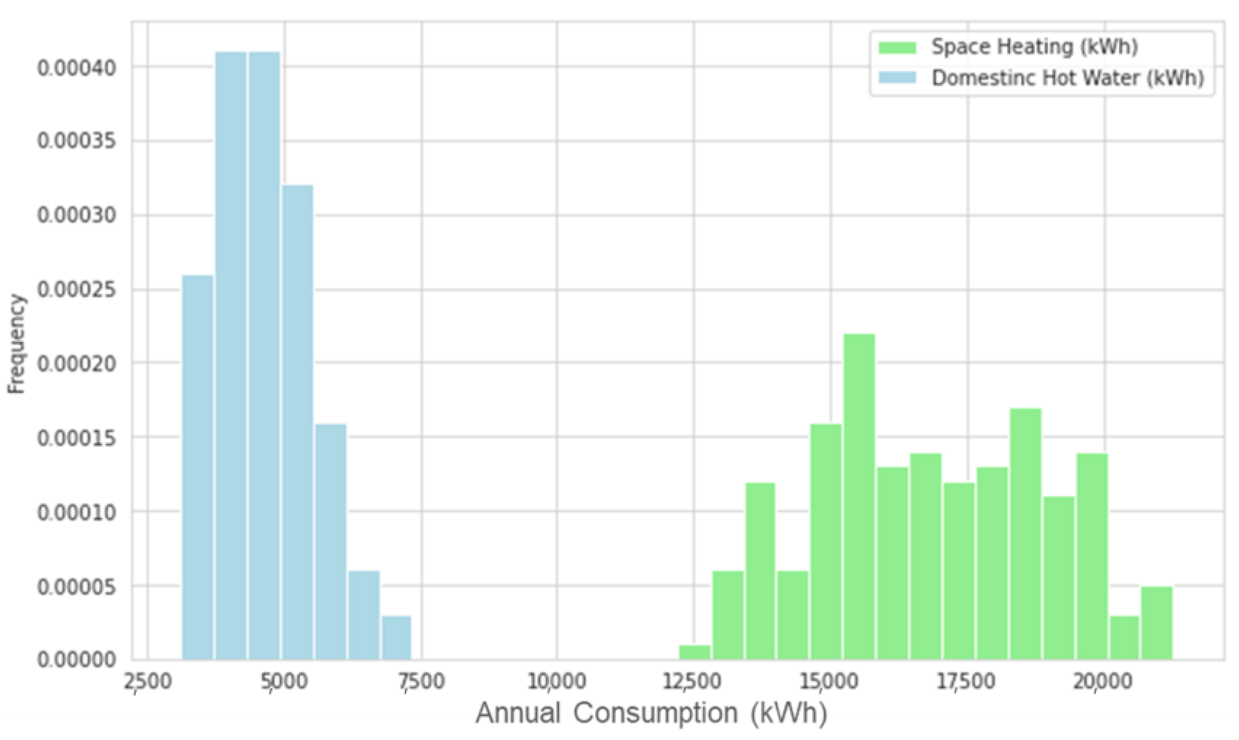
Figure 10 shows the frequency of DHW and SH energy demand within the case studies of this research. The outcomes indicate a trustable and stable prediction of the energy decomposition on a large scale. Hence, the results are also very insightful for large-scale analysis and decision-making. On the country scale, making case-specific decompositions helps in developing accurate bottom-up models. It can help in understanding the main source of inefficiency and find tailor-made solutions.
The total heat use below the CPT includes DHW and SH. Hence, the ESC of the total gas consumption is shifted by a certain constant to formulate the SH consumption. This shift is set as the minimum value in the ESC model as 2831 kWh. Since there are no means of validating the SH and DHW end-use models individually, we calculated the total heat demand using individual ESCs of SH and DHW and then validated the predictions using the total gas meter readings. For the yearly data sample, the coefficient of determination (R2) between the model and the measured gas consumption is calculated to be 0.94 and the root mean square error is estimated to be 19 kWh. Although this indicator can be promising and insightful, it is not reported as sufficient indicator for cross-validation of the outcomes on a large scale, since the model was tested with its training set.
4. Discussions
A comparison of HLCs estimated using different methods reveals that the theoretical HLC was clearly larger than all other estimated HLCs derived from monitored parameters. HLC estimated using LR models is stable and represents actual building energy performance. This demonstrates that HLC estimation using LR models—having acceptable simplicity—can be a viable option for closing the performance gap while also being a practical method to be upscaled in building energy performance analysis. Note that the performance gap has been previously reported and discussed (e.g., [
40]) and it refers to a systematic deviation between the estimated EPC and the actual energy demand of a building. The discussion of the usefulness and practicality of monitored energy performance of the building is still ongoing. The ambiguity arises from the fact that actual consumption also reflects the behavior of occupants on the building energy performance. However, one can say that building energy performance must only reflect the building condition rather than the subjective use of it. In this regard, HLC methods can be a simple supplementary indicator for building energy performance.
It was repeatedly observed in the result section that the estimated HLC can come with low confidence. Considering results from the ESC method there is a significant disparity in the estimated HLC values, whereas there is minimal variation in the breakdown of space heating and domestic hot water components. As such, as a future research topic, this study proposes the use of an energy signature curve to initiate LR models for HLC estimation in an iterative procedure. However, ESC is a purely statistical approach that may be carefully coupled to LR models which are initiated by physics in this context. For instance, CPT is a statistical term and does not correspond to the physical attribute of the temperature before which heating is activated, while the slope of the graph is realized as HLC which corresponds to the estimated HLC for each case study.
ESC showed high stability and reasonable outcomes for energy decomposition. Hence, this method can be used in upscaled and unsupervised online applications where the energy performance of a building is analyzed using only time series of measured energy use. Additionally, based on the observations in this study, it is advised not to consider CPT as an independently meaningful parameter for reporting and comparison.
This decision about the appropriate method for energy assessment using metered parameters can be adapted for different case studies depending on the building parameters and climate. The main limitation is that specific outcomes can only be achieved with specific inputs. Hence, the lack of appropriate input data hampers the use of advanced methods, even with the proposed framework with a broad range of methods. Data enhancement methods are an intermediate step towards solving this issue, hence a future step for this study. Data enhancement methods such as synthetic data generation help the energy audits to enrich the dataset and apply the proposed methods.
Table 3 summarizes the proposed methods and provides a guide to finding the appropriate method considering the available input data and expected outcomes.
5. Conclusions
With the increasing focus on achieving a carbon-neutral future, there is a need to explore energy-efficient solutions for the built environment besides the conventional building stock renovation measures. Furthermore, such solutions should focus on enhanced customer awareness and engagement at the local community level. Over the past decade, a focus on reducing energy bills, and creating engaging and personalized content has led to an explosion in interest in energy disaggregation to identify and quantify specific sources of household energy use. Often, the implementation of energy disaggregation poses a significant implementation risk for building managers and energy service companies as there is a lack of a holistic framework to guide the involved stakeholders.
With the increased adoption of smart meters, it has become relatively easier to explore disaggregation at the individual building and urban scales. Disaggregating the smart meter data further provides insights into composite end-uses and consumers’ energy usage habits. As the meters provide data on an aggregated level, the disaggregation process uses physics-based, hybrid, or data-driven techniques to break the original data into end-use components. This process uses different layers of data from other sources such as the weather data to devise unique energy signatures and statistical patterns of different components such as domestic hot water, space heating, space cooling, and electrical appliances.
This research proposes a data-driven framework that sets the guidelines to implement various disaggregation techniques considering the type of data available for the analysis. The demonstrated techniques calculate different end-uses namely building space heating, space cooling, domestic hot water, ventilation, lighting, and PV self-consumption. The disaggregation techniques include calibrated theoretical energy decomposition, HLC, and ESC using energy bills. These techniques function on the basis of data availability at the individual building level. For instance, while the calibrated theoretical energy decomposition technique mainly uses yearly aggregated energy bills, the energy signature curve makes use of hourly electricity and gas consumption data. As the main outcome of this article, the presented methods have been summarized in a table so that the reader can decide on the appropriate method considering the expected outcomes and limitations of the input data.
The results establish the importance of case-specific energy decomposition and the usefulness of measured energy performance indicators. The calibrated theoretical energy decomposition requires knowledge of the building’s physical parameters. Hence, alternative methods based on data-driven techniques were provided for energy decomposition.
Comparison between the outcomes of different LR models and ARX models shows higher stability in LR models in the results of this study. The challenges of selecting a reliable ARX model, affected by factors such as model order, data sample time, and parameters make the ARX model complex and prone to cumbersome tuning tasks. ARX models have larger confidence intervals but can significantly alter the identified HLC. Hence, they cannot be used in standardized applications in which different buildings are compared based on their reported energy performance derived from the ARX approach. ARX remains appropriate for research applications to answer specific questions such as the impact of building design on its thermal dynamic behavior. Moreover, ARX is appropriate for case studies with significantly high solar gains and internal gains such as office buildings with high glazing area. On the other hand, linear regression models provide more reliability checks and are flexible since the complexity can be increased to incorporate multiple parameters if data are available.
The ESC method facilitates remote energy analysis for upscaled retrofit recommendations. The results indicate the formulated models represent the generalized trends of space heating and domestic hot water end-uses. Moreover, this method provides an indication of total heat end uses in buildings where only one gas meter is available. The end-use profiles would eventually serve as an instrument to prove personalized recommendations and improve the energy efficiency of buildings. The method’s novelty is the possibility of applying it to hourly heating measurements without in-depth knowledge of the building and its occupants. This method is computationally cheap and can be implemented in online platforms to present simple energy analysis when receiving simple inputs to serve public audiences. CPT, as the temperature after which the heating is deactivated, derived from ESC is not a physically meaningful parameter and cannot be used to explain the building energy performance or user behavior.
Future work could focus on the implementation of the demonstrated techniques with other datasets for further validation and robustness analysis given the datasets represent varied climates. ESC method is a computationally fast and cheap method that can aggregate urban scale datasets such as income distribution in the energy disaggregation market at large. This would create additional opportunities for lower-income households that are dedicating larger percentages of their paychecks to utility bills.

 ,
, 


