Modelling and Estimation in Lithium-Ion Batteries: A Literature Review


1
ETSEIB, ESAII, Universitat Politécnica de Catalunya, Avinguda Diagonal, 647, 08028 Barcelona, Spain
2
Insitut de Robòtica i Informàtica Industrial CSIC-UPC, C/Pau Gargallo, 14, 08028 Barcelona, Spain
*
Author to whom correspondence should be addressed.
Energies 2023, 16(19), 6846; https://doi.org/10.3390/en16196846
Submission received: 31 July 2023
/
Revised: 20 September 2023
/
Accepted: 25 September 2023
/
Published: 27 September 2023
(This article belongs to the Section D2: Electrochem: Batteries, Fuel Cells, Capacitors)
Abstract
:Lithium-ion batteries are widely recognised as the leading technology for electrochemical energy storage. Their applications in the automotive industry and integration with renewable energy grids highlight their current significance and anticipate their substantial future impact. However, battery management systems, which are in charge of the monitoring and control of batteries, need to consider several states, like the state of charge and the state of health, which cannot be directly measured. To estimate these indicators, algorithms utilising mathematical models of the battery and basic measurements like voltage, current or temperature are employed. This review focuses on a comprehensive examination of various models, from complex but close to the physicochemical phenomena to computationally simpler but ignorant of the physics; the estimation problem and a formal basis for the development of algorithms; and algorithms used in Li-ion battery monitoring. The objective is to provide a practical guide that elucidates the different models and helps to navigate the different existing estimation techniques, simplifying the process for the development of new Li-ion battery applications.
1. Introduction
Lithium-Ion Batteries (LIBs) are currently the most popular Energy Storage System (ESS). Their high demand in electric vehicles (EVs) and renewable-energy-powered grids make them a device of great importance on the road towards decarbonisation of industrial societies. There are several reasons behind this popularity. First, their flexibility makes them suitable for aggressive, rapidly-changing applications such as electric vehicles (EVs), as well as for static and slow-changing cases like grid-connected storage or small applications such as laptops or phones. Moreover, their rotund-trip efficiency is typically rated between 85 and 95%. Additionally, LIBs offer a good balance between power density and energy density [1,2], and their cost has been decreasing as production increases.
There exist some notable alternatives to LIBs. Zinc-ion batteries are potentially safer and low-cost but are still in development [3,4]. Lithium-selenium batteries are another emerging technology with potential for high energy density [5]. Aqueous ammonium-ion batteries are environmentally friendly, with potential for static applications [6]. Supercapacitors are characterised by a low energy density and can therefore be applied to fewer applications if not combined with other ESS [7]. Finally, vanadium redox-flow batteries are suitable for static applications, as power can be decoupled from energy [8,9]. Compared to the alternatives, LIBs emerge as a mature and versatile technology in terms of energy and power density, as well as the number of applications.
Lithium-ion batteries do not refer to a single type of device. Instead, there is a wide variety of chemistries and mechanical formats, each with different characteristics [10]. While the working principles of these batteries are the same, commercial cells use different materials for the cathode and anode. Moreover, LIBs can come in multiple formats, the most typical of which are cylindrical, prismatic and pouch cells.
To successfully implement a battery system in a real application, the use of a battery monitoring system (BMS) is needed. BMSs are used to monitor and manage several states of the cell to keep the battery in safe and efficient conditions and actuate in case of abuse or malfunctioning [11,12]. To do so, estimation algorithms must compute the cell status using available measurements, such as temperature, voltage and current, as well as a mathematical description of the system dynamics. Hence, battery modelling is a key part of the estimation design process. The development of control-oriented models in recent years has led to a myriad of modelling approaches, which can usually be classified into electrochemical-based models, equivalent circuit models (ECMs) and data-driven models [13,14]. The differences between diverse models are discussed in this paper. A general idea is that the closer the model is to the real physics of the cell, the more detailed the description of the battery behaviour but at the expense of increased computational cost. In an attempt to maintain the benefits of an accurate model while sufficiently reducing the computational cost for real-time applications, many simplification methods have been developed in the literature.
With knowledge of the behaviour of the battery, the next step in its management is the estimation of unmeasured internal variables. Typically, state of charge (SoC) and state of health (SoH) are key indicators of the cell that cannot be directly measured. Battery parameters also play an important role in battery management. While they vary slowly (typically due to aging processes), obtaining information about them is highly desirable. While some offline experimentation or open-loop calculation (i.e., Coulomb counting for SoC calculation [15]) can provide an approximation, the online closed-loop estimation of these indicators is crucial for robust and accurate real-time monitoring. However, the large variety of estimation algorithms can make the choice of a concrete algorithm difficult. Some approaches are based on data-driven models that operate by means of machine learning algorithms. Other procedures rely on the use of observers. While variations in the extended Kalman filter (EKF) [16,17,18] or other linear observers are widely used, the use of a linear observer to estimate the states of a nonlinear system can result in failed estimation if the initial state of the algorithm is far away from the current state of the cell [19]. To address this, nonlinear observers can be a better solution if their inherent difficulties are successfully overcome.
The contributions of this article can be summarised as follows:
- Insight is provided on the fundamentals of Li-ion batteries regarding the main and side reactions, with the aim of explaining the basics in a comprehensive way;
- The modelling of LIBs is summarised and explained in a straightforward way from a state-estimation perspective;
- A complete single-particle model (SPM) is provided, as well as a review of the simplification methods for electrochemical models. Finally, the proposed SPM is simplified to extract a reduced order state-space model;
- A picture of the landscape of observers is provided, with explanations of the strengths and weaknesses of each mentioned observer, again with the intention of comprehensively elucidating the fundamentals;
- A classification of estimation methods is provided for SoC and SoH.
The article structure can be found in Figure 1. In Section 2, the fundamentals of LIBs are discussed, with mentions of potential side reactions and the provision of some indicators. Additionally, a comparison between different Li-ion chemistries is included. Section 3 covers the modelling of LIBs, and models are classified as electrochemically based ECM and data-driven models. Furthermore, we provide a brief discussion about the simplification of electrochemical models from a control perspective. Finally, Section 4 provides an overview of the estimable information for LIBs and a definition and justification for observers. Moreover, we offer an account of observers used in LIBs.
2. Fundamentals of Li-Ion Cells
In this section, we provide a general description of the working mechanisms of a Li-ion battery, followed by a summary of the indicators to be taken into account to monitor the battery.
2.1. Working Principles
Lithium-ion batteries are composed of three essential components: a positive electrode known as the cathode, a negative electrode known as the anode, an electrolyte and two current collectors. The cathode is typically made from lithium metal oxide, while the anode is commonly constructed using graphite or other carbon-based materials. The electrolyte is a solution that contains lithium salts. The current collectors are responsible for conducting the electrical current outside the battery, serving as an interface between the cell and the external circuit.
Simply put, a battery is an electrochemical device that is capable of bidirectionally transforming chemical energy into electrical energy. This conversion is achieved through a bidirectional process involving the electrolyte stored within the battery electrodes. The interface connecting the electrode and electrolyte facilitates reduction–oxidation reactions [20], as shown in Figure 2.
When a current flows through the battery, the oxidation reaction releases electrons, which are then directed through the external circuit by the reduction reaction. Simultaneously, ions released from the electroactive species travel between the positive and negative regions of the battery, facilitated by the movement of the electrolyte.
The battery voltage is measured as the difference in potential between the current collectors and is related to the concentration of intercalated in the electrode particles (see Section 3.1.4).
The main reactions, described in a general form for a carbon anode, are (1) for the charge process and (2) for the discharge process.
where is the general form of the cathode chemistry, as an oxide of a metal (M), and n and m are the stoichiometric coefficients of lithium involved in the reaction. During the charge, lithium ions move from cathode to anode through the electrolyte, while the electrons move through the external circuit. During discharge, the process is reversed.
Typically these reactions are exothermic, as the transport of lithium is associated with heat generation. A comparison of different materials for LIBs is provided in Section 2.4. As an example, for a cathode of and a carbon anode (see Section 2.4), the equations would be:
Figure 2 facilitates the visualisation of the structure of the cell, as well as detailing where and when reactions happen. The external circuit is also depicted.
2.2. Side Reactions
Side reactions occur within LIBs and differ from the main reactions described in Section 2.1. These side reactions have the potential to occur under specific circumstances, and their effects can be potentially harmful. Many of these reactions appear when the battery is excessively charged (overcharged) or almost discharged [14,21]. The former usually generates a high output voltage, while the latter generates a low output voltage. While only an overview is provided here, more information on degrading side reactions can be found in [22,23]. Finally, a detailed mathematical model is found in [24]. A summary of side reactions can be found in Table 1.
2.2.1. Overvoltage
During the charging process of LIBs, lithium ions () migrate from the positive electrode to the negative electrode and intercalate within it. This process increases the cell’s potential. However, if the battery undergoes a strong overcharge (a situation that occurs when the stored charge is close to or in excess of the battery capacity), the cell potential can rise to a point where the following phenomena occur.
- Lithium plating: The graphite electrodes become saturated with lithium, leading to an effect known as lithium deposition or lithium plating. This results in the formation of dendrites within the anode, which obstruct the flow of ions. Over time, dendrites can extend into the separator, causing short circuits [25,26].
2.2.2. Undervoltage
On the other hand, a sudden voltage drop appears when the battery is overdischarged. In this situation, the properties of the electrolyte change, creating an effect known as solid electrolyte interphase (SEI).
- SEI: An undervoltage situation leads to the precipitation of insoluble products onto the electrode surface in the anode, forming a passive film known as the SEI. While the SEI is necessary to prevent unwanted reactions between the electrolyte and the electrode, it is convenient to avoid the excessive growth of the SEI, as it can also contribute to capacity fading [28,29].
2.2.3. High Currents
A current much greater than the nominal current of the cell can also have a negative effect:
- Particle fracture: The particles may change volume and thus stress the electrode materials. The effect of particle fracture can indirectly cause the growth of the SEI or loss of active material [30].
2.2.4. High Temperatures
Finally, high temperatures can influence the battery behaviour in two ways: first, as an accelerator for undesired reactions; and second, by melting the separator, creating internal short circuits or thermal runaway [23].
2.3. Indicators
The use of indicators that enable the evaluation and diagnosis of battery behaviour through monitoring is highly desirable. Consequently, the following indicators are usually defined.
- Capacity () [Ah]: The maximum amount of charge that can be stored inside the battery and delivered during a full discharge cycle. The capacity (usually expressed in Ah) varies according to the quantity of material in the electrodes;
- Nominal capacity () [Ah]: The original capacity of the battery when it is new and no degradation has occurred;
- State of Charge (SoC): The primary indicator in LIBs, providing information about the remaining energy inside the battery. SoC can be defined as in Equation (4), where Q is the actual capacity and is the maximum capacity of the cell, both measured in ;
- SoH: The ratio between the current maximum available capacity and the rated available capacity, which indicates the battery’s aging condition. It can be expressed mathematically as follows:
- C rate: The charging or discharging current relative to capacity. A 1C rate corresponds to full charging or discharging the battery in one hour, while 0.5C corresponds to two hours of charging. The C-rate for a 2 Ah cell being charged or discharged at 2 A is 1C, and if the current were 6 A, it would be 3C. In general, a value above 3–4 C is considered a high C-rate, although this varies notably depending on the chemistry.
2.4. Li-Ion Materials
According to [10], LIBs can be categorised into several categories depending on the electrode material. In the case of negative electrode materials [10], carbon-based and lithium titanate electrodes (LTO, ) are the most common materials for LIBs.
The most common positive electrode materials [10] are lithium cobalt oxide (LCO, ), lithium nickel oxide (LNO, ), lithium manganese oxide (LMO, ), lithium iron phosphate (LFP, ), lithium nickel manganese cobalt oxide (NMC, ) and lithium nickel cobalt aluminium oxide (NCA, ). x and y refer to the particular alloy used by manufacturers, which may vary. The material in the cathode is mainly responsible for the battery cost and performance in terms of energy, power, lifespan and safety, as shown in Table 2, where different families are compared with on a scale of 1–4. In [10], a comparison was made in terms of cost, energy (Ah), power (W), safety, lifespan and performance. While cost, capacity and power are measurable quantities, the rest of the variables require further explanation. Safety can be related to the temperature at which the cell degrades beyond recovery in what is known as the thermal runaway; the highest temperature of the thermal runaway corresponds to the highest cell safety level. Lifespan is directly computed based on the number of cycles that a cell can withstand. Finally, performance refers to the behaviour of the cell at hot and cold temperatures, where typically capacities are reduced [31,32].
3. Modelling
In order to achieve the estimation of key indicators, it is essential to have a mathematical model that can accurately represent the behaviour of the system, which, in turn, provides a comprehensive understanding of the interconnected working principles. Finally, mathematical models serve as a basis for the development of real-time control, estimation and monitoring algorithms. There exists a wide range of models for LIBs, varying in complexity and level of detail. Naturally, the computational time and feasibility are directly related to the complexity of the model.
Such models can be classified as follows [13].
- Mechanistic models are based on the physical and chemical phenomena occurring within the battery, providing a detailed, accurate and interpretable representation of its internal behaviour.
- ECMs simulate the causality between the battery current and the voltage by constructing an electric circuit using resistors and capacitors, although they do not inherently represent the physical effects.
- Data-driven models are developed solely based on measured data and with minimum to zero use of the battery first principles, which makes them less effective in describing internal physicochemical phenomena. However, they have the potential to capture complex behaviour that is not yet fully understood from a physical perspective.
3.1. Mechanistic Models
When discussing mechanistic models, one can delve deep enough to the point of treating each particle individually. Although these models can be valuable in material design for batteries, they may not be practical for operational purposes, especially when conducting whole-cell simulations over time. In such cases, simpler models that treat the battery as a continuous medium rather than accounting for individual particles are necessary. Typically, mechanistic models incorporate distributed behaviour, which refers to the spatial distribution of system variables and parameters. However, when it comes to control and estimation applications that require dynamic models, further simplification is required (see Section 3.1.5). In this section, we present a concise overview of microscale and homogenised models that serve to illustrate the simplification of physics prior to reaching the Doyle-Fuller-Newman (DFN), also known as the Pseudo2-dimensional (P2D) model, which is probably the most popular and foundational model for simplified representations. A single-particle model (SPM) is a simplified version of DFN, but as it still employs distributed parameters, we present certain simplifications in Section 3.1.5. A simple comparison of the mentioned models is provided in Figure 3.
Before continuing, a necessary clarification must be made. It has been stated that mechanistic models incorporate the spatial distribution of system states, which necessitates consideration of the dimensions of the cell models. A battery is a device with three spatial dimensions, but it does not always need to modelled by considering all three dimensions. Of the models presented in this section, the microscale and homogenised models can be used to describe the battery in two or three spatial dimensions; the DFN model is, as mentioned, pseudo-two-dimensional, and the SPM is essentially one-dimensional.
3.1.1. Microscale Model
The first model that must be mentioned is the microscale model, which offers a continuous description of charge transport at the level of individual electrode particles [33]. This model serves as the basis for other battery models and requires an accurate microstructural representation. It encompasses the transport of lithium ions and electrons within the electrodes, as well as the role of the electrolyte in facilitating ion and charge movement. However, the computational requirement of determining the geometry of each electrode particle presents a significant hurdle to overcome.
The concentration of lithium intercalated in the electrode molecules in the cathode and anode is known as the solid phase. Despite the difficulty of determining the geometry of the particles, solid transport is commonly modelled using a diffusion equation, which allows for the quantification of the concentration at each point of the electrode (see Figure 3). Concerning the electrolyte, as it is responsible of the transport of the lithium ions (), it can be directly coupled with the charge flow. Finally, the Butler–Volmer equation is utilised to capture the exchange of lithium ions between the electrode particles and the electrolyte [14].
Diffusion demonstrates the multidimensional characteristic of this model, as well as how other models simplify this phenomenon. Diffusion is modelled using Fick’s second law of diffusion [34], as expressed in a general three-dimensional form in Equation (6):
where c is the concentration; x, y and z are the spatial coordinates; and D is the diffusion coefficient, which is dependent on x, y and z, as well as the concentration. We return to this example for explanation of the subsequent models.
3.1.2. Homogenised Model
A simplification of the microscale model can be obtained by assuming that the porous material and its spatial structure form a uniform continuum. This simplified approach [35], known as a homogenised model, can be achieved based on the solutions of the microscale model, which indicate that several variables do not significantly vary over the length scale of the microstructure. To carry out the simplification, averaged variables and effective parameters are employed instead of relying on the spatial region. Following the example introduced in (6), here, as we assume that the solid phase is homogeneous and that the diffusion coefficient no longer depends on the spatial coordinates but only on the concentration.
More information about the microscale and the homogenised models can be found in [14]. With some additional simplification, the DFN model can be achieved.
3.1.3. Doyle–Fuller–Newman Model
The DFN model [36] is arguably one of the most popular mechanistic models for lithium-ion batteries. Evidence of its popularity can be found in various derivations (SPMs) and its applications in the field [37,38,39,40].
The DFN model is derived from the aforementioned homogenised model but with the assumption that all particles are perfectly homogeneous spheres, thereby eliminating the need to compute the geometry of each particle. Additionally, the electrodes and separator are considered to have a one-dimensional geometry, simplifying the equations to be solved on a one-dimensional axis (typically the horizontal axis). As the morphology of the particles is typically unknown, these assumptions significantly facilitate the characterisation of the cell.
- Solid Phase
Returning to the example of (6) and (7), Fick’s second law can be applied to perfect spheres using spherical coordinates, as shown in (8), setting the origin at the centre of the particle:
The angle variations (the terms relative to the angle ( and )) can be neglected, as the particles are assumed to be homogeneous and the variation inside a particle only depends on the radius. This is reflected in the following equation.
where c is the concentration of the solid phase, D is the diffusion of the solid phase and r is the radius of the particle. A complete summary of the nomenclature used can be found in Table 3.
Note that here, the concentration in each particle only depends on the radial distance to the centre of the particle, but there are several particles distributed along the x axis (as in Figure 3). Thus, the model can be called pseudo-two-dimensional, as it depends on two axes that are not independent of one another.
In Equation (9), the boundary conditions must be evaluated at the radial coordinate ( or , where is the radius of the particle; see Figure 4) [41].
When , the constraint results in solid particles that cannot diffuse from the centre of the particle, as the mass would disappear as in a black hole, which would break the conservation-of-mass assumption inside each particle.
When the radius is that of the particle (, see Figure 4), diffusion occurs in the form of flux of lithium ions, which are linked to the current that charges or discharges the battery. This boundary is held by the assumption that the particles (de)lithiate uniformly, which means that lithium ions (de)intercalate in the solid at the same rate.
where j is the molar flux and F is the Faraday constant.
- Electrolyte
In order to define the DFN model with respect to transport in the solid and electrolyte phases, further explanation is required.
The electrolyte is in charge of the transport of diluted lithium ions across the whole cell. As shown in Figure 3, it permeates the three areas of the cell. Figure 5 represents the cell, focusing only on the electrolyte. It is important to understand the limits of the spacial coordinates.
The governing equations are introduces as follows. Mass transport in the electrolyte can be described using (12) [14,42], which is based on mass balance for the whole cell.
where is the transference number (, the fraction of the current carried by positive ions [14]); is the porosity; and is the electroactive surface area, which can be described as , where is the active volume fraction of solid phase. A slight variation of Equation (12) can be found in [41], where depends on .
The first term on the right-hand side of (12) can be thought of as the change in concentration due to diffusion [37]. Notice that the first term comes from Fick’s second law of diffusion (6), ignoring the diffusion on the y and z axes. The second term reflects the change in concentration due to variations in current. As the electrolyte permeates the whole cell, (12) must be applied to the three regions, but as in the separator, there is no charge transfer, so the last term of (12) disappears.
The boundaries of Equation (12) can be evaluated at the extremes of the cell and at the extremes of the three different areas. In the first case, Equation (13) prevents the diffusion of electrolyte outside the cell, which would result in its destruction.
To reflect the fact that the electrolyte permeates the entire cell and that, therefore, the flux and concentration are continuous between electrodes and separators [37], the evaluation of Equation (12) in the region where the electrodes meet the separator is expressed as Equation (14), indicating that force is continuous, with uniform flux between the anode, separator and cathode.
where x and L are the same as in Figure 5.
With this set of equations, the DFN model is complete. In [14], a complete derivation from the homogenised model was provided. The missing parts required to determine the described behaviour of the whole cell are the cell voltage and the thermal model. However, for the sake of simplicity, they are only described for the SPM, as there is no simple way of describing them without the assumptions of the SPM.
3.1.4. SPM
Diverse simplified versions of the DFN model fall under the SPMs, still written in the form of PDE but significantly simpler computationally. The main assumption of these models is that a single particle can be representative of the whole electrode, assuming that the behaviour is similar across multiple particles.
Therefore, according to [43], the assumptions under which the SPM is derived from the DFN model can be summarized as follows:
- The concentration of solid particles is homogeneous in a radial sense so that the concentration only varies on the radial coordinate (r);
- The current density in each electrode is uniformly distributed;
- The number of moles in the electrolyte and that in the solid phase are both conserved. This can establish a proportional relation between current and flux;
- The transport coefficients () of the anode and cathode are equal.
The diverse ways in which the DFN model has been simplified has led to a wide variety of SPMs that can be classified, according to [14], as those take into account the electrolyte dynamics (SPMe) [44] and those that do not [45].
However, all of these methods the same working principles and the same governing equations. Figure 6 shows the simplest representation of the cell, with only one particle in the anode and cathode, respectively, and three separated regions.
In summary, the SPM can be established as a 1D geometric model that only depends on the spatial coordinate (x) in the electrolyte or the radial coordinate (r) in the solid phase. The model has three separate areas and considers flux as homogeneous. Mass transport in lithium ions and the electrolyte are needed to successfully describe the model.
Due to the aforementioned assumptions, the subsequent equations describe an SPM, describing first the diffusion in the solid phase, as well as taking into account electrolyte dynamics. After describing the diffusion phenomena in the three areas, we explain the cell potential. We also provide a brief discussion about incorporation of the effects of temperature in the SPM.
- Solid Phase
As mentioned, the dynamics of the concentration in the solid phase can be described using Fick’s second law of diffusion, which serves as an example to illustrate the simplification from the microscale (6) model to here. Equation (9) can be rewritten in a simpler way using the chain rule as:
Note the suffix i, which refers to the negative electrode or the positive electrode, and the suffix s, which reflects the fact that the parameter or variable is related to a solid. This notation is used later in this paper. is assumed to be constant under the assumptions according to which the SPM model is derived. Therefore, ; however, if this assumption were not considered, it would be a function that depends on .
The boundary conditions in Equation (15) are the same as those in (9); however, as current is proportional to flux (according to SPM assumptions), when the radius is that of the particle (, see Figure 4), the boundary condition can be rewritten as:
where F is the Faraday constant, is the electroactive surface area, A is the cell area and is the thickness of the region i (see Figure 4).
- Electrolyte
In the SPM, where electrolyte dynamics are considered, the general equations are similar to those of DFN. As mentioned, SPM assumes that the flux is proportional to the current, which enables (12) to be rewritten as:
The boundaries are the same as in DFN, as described in (13) and (14). We note that (17) must be evaluated in the three areas, but as there is no charge transfer in the separator, the last term would disappear.
- Cell Potential
The remaining issue concerning the governing equations for the cell is the potential. The potential can be measured between the two current collectors and is the effective voltage that affects any device connected to the cell. A typical curve of the cell potential is shown in Figure 7, for an LFP cell.
(18) is a general equation based on [14,41].
where U is the Open Circuit Voltage (OCV), is the overpotential, is the drop in potential in the electrolyte and is the film resistance related to SEI.
Overpotential () is calculated using different approaches in the literature. In the case of [43], the solution was computed as:
Different approaches are available to solve the Butler-Volmer (B-V) relation:
In (19) and (20), R is the gas constant, is the transport coefficient (previously assumed to be equal for both the anode and cathode) and is the exchange current density.
The potential drop in the electrolyte () is also expressed in several ways in the literature. Again, according to [43]:
where is the diffusional conductivity, as reported in [37,43] as a function dependent on the electrolyte concentration that can be approximated as a uniform parameter if assumed to be constant in the space. On the other hand, the authors of [41] defined as an empirical equation. is defined in (22). On the other hand, the authors of [14,47] completely neglected the effect of the concentration on the drop in potential of the electrolyte.
where is the effective solid conductivity, typically defined in the literature according to Bruggeman’s relation [14,41,43,47] as . Bruggeman’s relation refers to the effective conductivity inside the microstructure of the cell.
- Thermal Modelling
The SPM presented earlier is treated as isothermal, but the temperature cannot be neglected. Thermal management is also a popular topic; therefore, thermal modelling has been widely discussed in the literature [48,49,50,51]. However, predicting the temperature is highly complicated, as heat generation is nonlinear and thermal properties are anisotropic. Moreover, a commercial cell is large enough to exhibit a temperature gradient throughout the entire cell. Hence, the temperature variation becomes a three-dimensional problem, given the significant temperature variation across the structure. This results in a five-dimensional model in the case of a DFN thermal model or a four-dimensional model if the SPM is used.
Nevertheless, it has been found that lithium diffusivity, reaction rates, and electrolyte diffusivity and conductivity can be described by the Arrhenius relationship, as expressed in (23).
This relation was used in [41,48] to extract a temperature-dependent SPM. While the authors of [48] neglected the electrolyte voltage drop, the authors of [41] considered it. In both of the abovementioned studies, OCV was considered temperature-dependent as follows:
In other works, such as [47], a purely empirical equation is provided.
3.1.5. Finite-Order Models
Several methods are available to transition from a physics-based model, such as the DFN, to a simpler and more manageable model for control-oriented purposes. One apparent approach is to employ a simplified physics approach, resulting in the SPM, as discussed in Section 3.1.4. However, it should be noted that the SPM remains an infinite-order model, as it is described using PDEs.
To successfully represent a system, such as in a state-space representation, a finite-order model is necessary. In response to this requirement, several simplification techniques have been developed. The authors of [42] reviewed the techniques used in the literature to achieve such reductions and classified them in the following families.
- Spatial discretization: Well-known techniques such as Finite-difference Method (FDM) or Finite-volume Method (FVM) are used;
- Function approximation: Spatiotemporal variables are approximated by a finite weighted sum of assumed trial functions that are fitted using optimisation techniques;
- Frequency domain approximation: The frequency response is obtained means of Padé approximation or the residue grouping method, among other techniques;
- Physics simplification: Typically achieved using diverse SPM approaches with several variations.
- Spatial Discretization
The spatial coordinate is discretized to obtain a continuous-time description, making it suitable for control applications. This strategy is also known as the method of lines. The most common and direct methods of spatial discretization are the finite-difference method [52] and the finite-volume method [53]. These methods can preserve most model properties within a wide range of conditions. The main difference between them is that FVM is mass-conservative. However, their complexity lies in the number of control volumes or mesh points used. In the appendix of [12], the general equations for discretization using FVM and FDM are provided. Here, the equations for FVM are presented in (26). The difference between FVM and FDM can be seen in Figure 8. FVMs are mass-conservative, since they enforce the conservation principle and balance the net flow of conserved quantities, while FDMs lack explicit conservation enforcement within their discretization.
- Function Approximation
The behaviour of the model is approximated by a function that has time-varying coefficients, approximating a trial function dependent only on the spatial variables. These functions can be polynomials, sinusoidal, logarithmic or a combination of several thereof. These methods are also known as projection-based methods, and the fitting of the parameters or trial functions is achieved using optimisation techniques. An example can be found in [54], where a decomposition of the data from the original DFN model is presented. If instead of minimising the error, it is integrated and weighted over the evaluated domain such that the result of the integral is zero, these methods can be referred to as spectral methods. The renowned Galerkin method also falls into this category [55].
- Frequency Domain Approximation
Various approaches are available to obtain the frequency response of a system. The eigenfunction technique [56] calculates all periodic roots of the transcendental function, truncating the infinite series to obtain a finite-order model. The residue grouping method [57] also calculates and truncates periodic poles and zeros, grouping poles and approximating them through frequency response cost function optimisation. While residue grouping offers improved accuracy across a broad frequency range, it is less suitable for real-time systems due to computational inefficiency, sensitivity to initial guesses, and lack of guaranteed convergence and global optimality.
In contrast, Padé approximation [58] linearises transcendental transfer functions into rational ones in the s domain, allowing for direct system order reduction through moment matching. The rational polynomial coefficients incorporate physical cell parameters and can be easily updated for operational changes. Higher-order Padé approximations provide increased accuracy at the expense of additional computational requirements, making them suitable for EVs, while low-order approximations suffice for stationary battery applications.
- Physics Simplification
After discussing the SPM in Section 3.1.4, there is little left to discuss regarding physics simplification. However, Ref. [59] presents a different simplification of the DFN model in which the electrolyte concentration remains constant and the diffusion equation of the solid is approximated.
Before continuing, let it be noted that considering the equations, it becomes evident that the SPM is not a finite-order model. One potential solution is provided in [41], where the FDM is applied to the SPM.
Another option is the use of the FVM instead of the FDM, which offers the advantage of conserving mass. This document provides the discretized equations and the state space representation (see Section 4.4) using the mentioned method for a set of two control volumes per particle and three control volumes for the electrolyte, as seen in Figure 9.
- Concentration in the Solid
With boundaries (10) and (16) and applying the FVM with Equation (26), the concentrations for the solid in the four control volumes shown in Figure 9 can be obtained using Equation (15).
The concentration in every control volume is dependent on itself, as well as the concentrations of its neighbours.
- Concentrations in the Electrolyte
With boundaries (14) and applying the FVM with Equation (26), the concentrations for the electrolyte in the three control volumes shown Figure 9 can be obtained using Equation (17). Note that when (17) is applied to the separator, the second term disappears, as there is no mass transfer in that area. This implies that (32) is not dependent on the battery current.
3.2. ECMs
ECMs are, as mentioned, electric circuits designed to mimic the behaviour of a battery. Although they do not inherently represent the internal states of the battery, their simple form makes them easily understandable for non-experts on the topic.
The authors of [13] established two subcategories of ECM: those that are based on the electrochemical process and those that are not.
3.2.1. Phenomenological ECMs
Phenomenological ECMs represent a simple and popular way to reproduce battery dynamics without considering internal phenomena. Easily scalable, they usually takes the shape of an ideal voltage source corresponding to an OCV, series resistance and a variable number of RC nets. This can be seen in Figure 10, where a first and second order are presented. The models are scaled-up by adding more RC nets. The order of the model and, thus, its accuracy can be increased at the expense of computational effort [60].
A comparative study of the ECM family applied to several cell chemistries was reported in [60]. Experiments showed that the first-order model achieved superior accuracy on the performed tests.
3.2.2. Electrochemical ECM
The equivalent circuit aims to replicate the cell’s dynamics by incorporating electrical elements that recreate the battery’s structure. Since certain dynamics cannot be adequately reproduced by a simple RC network, the equivalent circuit also utilises ZARC elements (which account for the phase influence in the impedance and are represented by a net composed of a resistor and a constant phase element [61]) and Warburg impedances. ZARC elements are commonly employed to represent the SEI, while Warburg impedances are used to characterise diffusion. The use of these elements and their phase shape can are described in [13,62]. The use of these frequency-dependent elements requires precise characterisation. Electrochemical impedance spectra (EIS) is a method consisting of the application of a pulse of current or voltage to the cell of a determined frequency and amplitude and, with the phase shift and variation of amplitudes recorded. This yields the response of the cell in the form of a Nyquist diagram.
3.3. Data-Driven Models
Data-driven models utilise data to predict the behaviour of the battery. Their primary advantage is that there is no need to comprehend the complex physicochemical phenomena that determine the behaviour of a cell. However, the result of the model highly depends on the quality of data used for calibration.
The objective of data-driven models is to establish a relationship between measurable information about the battery and key indicators, such as SoC and SoH, commonly using machine learning algorithms to extract a model from data. Typical families of algorithms include artificial neural networks (ANNs), Gaussian process regression (GPR), linear regression (LR) and support vector machines (SVMs). To successfully develop an estimator using these techniques, measurements are needed in advance. Datasets are composed of inputs such as voltage, current or temperature and typically include the SoC as output. Models can be trained to extract an accurate output with respect to the past and present inputs. Depending on whether these models rely solely on data or employ a model (such as those described in the preceding sections, for instance) and data to calibrate it, the authors of [13] categorise them as black-box or grey-box models, respectively. Of the later, the combination of Kalman filter with one of the mentioned algorithms is a popular choice [18,63,64,65].
Clearly, the quality of the data used to train the models has a considerable impact on the accuracy of the estimation. The collection of these datasets can be a long process, as it may require long-term experimentation. It is also important that the accuracy of the data be compared to that required for the application in which the estimation will be used. In [66], some of the reviewed models were reported to use data that are not fully representative of the case under study. The process of training the models can also be a source of inaccuracy, as randomness is intrinsic to many machine learning algorithms. To overcome this situation, the authors of [66] recommend training the same model several times with the same dataset.
Without detailing of the myriad of algorithms that fall into the machine learning family (which are described in reviews such as [67,68]), here, we focus on the type of data used to train them. In the case of SoC estimation, while the authors of [69] relied solely on voltage and current, most methods [70,71,72] also use temperature. It should be mentioned that all these techniques require the “true” SoC for the training dataset. For SoH estimation, a greater number of combinations exists. Refs. [73,74,75] used only current, while the method described in [76] operates only using voltage. The authors of [77] employed both, whereas the authors of [78,79] considered temperature in addition to current and voltage. Finally, the authors of [80,81] relied on current, voltage and capacity.
Machine learning algorithms can also be used to forecast how a battery will behave in the future. The authors of [82,83,84] used different methods to predict a battery’s future behaviour using only information from a single cycle. The authors of [82] used voltage, current and SoC to estimate the trajectories of the remaining capacity and internal resistance. With the same goal, the authors of [84] employed the capacity and internal resistance of one cycle. On the other hand, the authors of [83] used voltage, current, capacity and temperature to estimate the remaining useful life (RUL), as computed in charge/discharge cycles.
4. Estimation in Li-Ion Batteries
4.1. Estimable Information
Estimation in Li-ion batteries is essential for proper battery management. Typically, the target is estimation of internal (and immeasurable) states, but estimation techniques also allow for estimation of information about system parameters, increasing the efficiency with which a model is adjusted. It is also possible to estimate parameters in online applications using a model that evolves with time and is therefore always accurate.
4.1.1. SoC
There are several ways to compute the SoC without using estimation techniques. Some observers use estimation techniques as part of their algorithms. However, each method has distinct disadvantages that, if used in an open-loop configuration, can cause errors.
- Coulomb counting method: Coulomb counting is the most straightforward approach to compute SoC in a cell. It involves integrating the current over time, thereby calculating the extracted capacity of the cell. However, this technique has two main drawbacks: the initial SoC is usually unknown, and the capacity may change depending on the C rate or the temperature, as well as the cell’s aging. Additionally, Coulomb counting is susceptible to various sources of error, as listed in [15], including current measurement error, current integration error, timing error, and measurement and process noise.
- OCV method: The OCV is closely related to SoC, meaning if one is known, the other can be determined. However, OCV can only be measured in the absence of current and after the battery has been at rest, as current causes voltage to deviate from the OCV curve, and due to hysteresis, it takes a long time to recover. Although this method is precise and straightforward, it is unsuitable for online applications. Nevertheless, it holds value in providing an OCV–SoC curve, as required in many models. The authors of [85] provided a detailed guide for OCV characterisation.
- Internal resistance method: By applying a fast current pulse and measuring the resulting voltage variation, the internal resistance can be determined and linked to SoC [86]. This method performs quite well at lower levels of SoC, where voltage tends to decrease rapidly. However, in other ranges, especially with a typical voltage plateau, SoC estimation becomes much less precise.
- Model and Look-Up table: Using a simple model properly experimentally calibrated under static conditions, OCV can be extracted. Then, for online applications, SoC can be computed using a look-up table that relates OCV to SoC.
More information about SoC computation can be found in [11]. A different path to SoC estimation is the use of observers. A discussion of the most suitable observers for LIBs is provided later in this section.
4.1.2. SoH
Several methods are available to estimate SoH using measurements.
- Internal resistance measurement: As a battery loses capacity and degrades, the internal resistance increases [87]. Periodically measuring it with current pulses, always at the same level of SoC, can provide information about the SoH. Internal resistance characterisation is an easier experimental method than capacity measurement and can be performed in a shorter time.
- Impedance measurement: Measurement of the impedance can also be related to SoH [88], as the battery impedance is affected by degradation. EIS is needed to characterise this phenomenon, providing valuable information, as electrochemically based models (Section 3.2.2) also use EIS to extract model parameters.
Other approaches involve the use of estimation algorithms, which lead to observation problems, as discussed in Section 4.2.
4.1.3. Parameters
Parameter identification for LIBs is a crucial process in understanding and characterising their behaviour.
Before continuing, we note the difference between parameters and states. While states are variables that evolve over time, are influenced by system inputs and are an indicator of the condition of the system, parameters are constant values that characterise the system. Parameters can change over time in response to changes in the system itself. In the case of LIBs, parameters may change due to aging.
When developing a model, the accuracy of its results depends on the selected parameters. Thus, parameter identification can be achieved through experimental testing and by later fitting experimental results to the model. Experimental tests involve the application of known inputs to the battery and measurement of its responses. These data are then fitted to appropriate mathematical models to extract the relevant parameters [89,90]. However, since temperature and aging can impact the cell’s behaviour, some approaches adapt the measured data to these two factors. This can be achieved both offline and online. In offline methods, the procedure involves conducting tests at different aging stages or temperatures ([91] to obtain an OCV–SoC–temperature relationship). Online parameter identification usually involves the use of estimation algorithms, which are discussed in the following sections.
Another important aspect related to parameter identification is the dynamics of the processes. For instance, charge transfer is significantly faster than diffusion processes. Estimation algorithms may take this into consideration and attempt to solve the identification task according to the appropriate dynamics [92].
4.2. The Observation Problem
Mathematical models of Li-ion batteries describe the dynamic behaviour of internal variables of the system, e.g., species concentrations or temperature, when a specific input profile is introduced to the system. This mathematical depiction allows for virtual simulation of the system which, in turn, can be utilised to further improve the design of Li-ion batteries. Another ambitious objective is the deployment of mathematical models that run in real time and in parallel with the true Li-ion battery. Real-time models can be used to retrieve information that, on the one hand, is not directly available from sensor measurements but, on the other hand, is necessary for control and monitoring of the Li-ion battery.
Up to this point, we have focused on presenting computationally efficient models that can be operated in real time. In this section, we focus on how to exploit these models and the measurements of available Li-ion battery sensors to retrieve internal information about the system. The process of estimating unknown dynamic internal variables from the measurement signals is commonly referred to as the observation problem.
In most cases, the observation problem is formulated using the state-space formalism; that is, the dynamics of the system are depicted through a multi-input, multioutput (potentially nonlinear) system in the following form:
where is defined as the state vector, that is, the vector of internal variables of the system. The states are not directly measured and are assumed to be unknown. The term depicts the vector of controlled inputs, that is, a set of signals that are measured and can be modified. The term is the set of measured signals. As a mathematical technicality and in order to simplify the analysis, it is common to assume that the vector functions are sufficiently smooth and that the solutions of the system in (34) are bounded and unique.
We define as the values of the states () of (34) at time t with the input profile () and initial condition (). Moreover, using this notation, depicts the value of the measured output () of (34) at time t with the input profile () and initial condition ().
In the so-called observation problem, the objective is to generate a time-varying signal (), which is defined as a state estimation, based on the known values ( and ) such that eventually converges to the true . One may wonder if this problem can be immediately satisfied by inverting the output equation, that is, by generating the estimation as
where is an inverse function of the output map (h) such that . However, Li-ion battery systems have fewer sensors than the dimensions of the state to be estimated (). Therefore, the inverse function () does not exist, and this solution is not feasible. This fact implies that a single sample of the output () is not sufficient to infer the states’ values. For this reason, the observation problem has to be solved using model in Equation (34) and the full trajectory of the measured signals ( and ) in the time range ().
The observation problem can be solved using different theoretical methodologies. As we assumed the solutions of the system (34), a solution to the observation problem is obtained by estimating the initial condition of the system (34) and forward simulating the model to generate the full state trajectory. A straightforward method to implement this idea is to forward simulate the system (34) for a set of different initial conditions and gradually eliminate all the initial conditions that do not agree with the measured signal (). This method can be implemented by means of a stochastic framework [93,94,95,96,97,98] (see [99] for more technical details about the approach) or a deterministic framework [100,101,102] (see [103,104] for more technical details about the approach). Moreover, under some observability assumptions, it can be proven that this method eventually retrieves the true initial condition. Although this is an interesting solution to the observation problem, it requires an adequate initialisation of the algorithm in a region around the true initial state. Moreover, the model of the system needs to be very accurate in order to achieve a precise forward simulation of the states.
Alternatively, the set of adequate initial conditions for the system can be computed by minimising a cost function online in the following form form [105,106,107,108]:
for some positive constant (T), time () and set (). Examples of this strategy in Li-ion batteries can be found in [109,110,111,112,113,114].
The limitation of this approach is that if the dynamics of the system are described by nonlinear differential equations (as is the case for Li-ion batteries), the optimisation in (35) becomes a nonlinear non-convex problem, which presents the obstacles of computational complexity, non-convexity and multiple local minima.
Up to this point, two possible routes for solving the observation problem have been presented. However, these routes are limited in terms of implementation in Li-ion batteries. Therefore, we need an alternative method to solve the problem.
Notice that the challenges involved in resolving the observation problem stem from three key factors: the unknown initial conditions of the system, uncertainties present in the analytical model and the nonlinearities within the model.
To begin with, the issue of unknown initial conditions can be addressed by ensuring that the algorithm’s trajectories ’forget’ their initial conditions over time. This characteristic can be seen as a stability property, where the error between the true states and the estimated states remains controlled.
In order to handling model uncertainty, the algorithm is required to exhibit robustness in the face of these uncertainties. Stability and robustness are fundamental concepts in control theory, which inspired the development of a state estimation algorithm incorporating the feedback concept. This specific algorithm is referred to as an observer.
Lastly, the matter of model nonlinearities serves as the motivation for designing an algorithm from a nonlinear control theory perspective and the development of nonlinear observers.
The main message of this section is that an observer corresponds to an adequate algorithm to solve estimation problems in Li-ion batteries. The remainder of this section is devoted to properly defining the concept of observer and proceeding with a review of observer-based techniques implemented in Li-ion batteries.
4.3. Observer Definition
Let us recall that the objective is to estimate the unknown states (x) of a system depicted by a model (34). The observer approach revolves around creating and employing a device known as an “observer” to generate real-time estimations, denoted as . Figure 11 illustrates the structure of observers.
In essence, an observer can be likened to a dynamic system that utilises the mathematical model of the actual system to replicate the state trajectories of the genuine plant. To compensate for model uncertainty, unmodelled disturbances and uncertain initial conditions, the observer incorporates a feedback component that adjusts the estimation by comparing the measured outputs with the observer’s estimations of these outputs. A more rigorous mathematical definition of an observer provided below (see also [115,116], [117] (Chapter 1) and [118] for more technical details on observer design for nonlinear systems). Consider the following set of dynamics:
where , with , is the observer state. The function is the output feedback term that satisfies for all . Finally, there exists a right inverse of the function such that for all .
Such a structure is an observer if it satisfies the following properties:
- as .
Notice that according to this definition of observer, we allow the following possibilities:
- The observer dynamics (36) are depicted in a different set of coordinates () than the original system coordinates (). Consequently, the observer includes a map () that relates the observer coordinates to the coordinates of the original system.
- The dimensions of the observer may be larger than the original system dimensions.
- Not only can the dynamics of the system be nonlinear, but the observer feedback term () may also be a nonlinear function.
4.4. State-Space Model of Li-Ion Batteries
In Section 4.2, observer development is commonly formulated by means of state-space representation. To successfully represent the battery model in state space, the system must be described in the following form:
In this case, the input (u) and the output (y) of the system are:
where V is the equation for the potential of the cell as expressed in (18), and is the battery current.
Therefore, is be a vector containing all the states (Equations (27)–(33)):
The equation for voltage (18) should be rewritten in a form that clearly indicates the dependencies on the current and on the states:
The expression for can be found in Equation (19). Finally, can be represented in the form of , where A and B correspond to the following matrices:
4.5. Observers in Li-Ion Batteries
In this section, we provide a review of observer techniques implemented in Li-ion batteries. Given the definition of observer provided in the previous sections, Figure 12 shows how the mentioned structural links to the battery model.
4.5.1. Linear State Observers
Although Li-ion batteries models are depicted by nonlinear differential equations, the model can be locally approximated by a linearly, which largely simplifies the observer design process at the cost of having to initialise the observer states “close enough” to the true battery states.
More precisely, the idea is to consider a pair that depicts a nominal trajectory of the nonlinear system to be observed. Then, first-order Taylor expansion of system (34) around leads to a linear time-variant system:
Then, since (43) is a good linear approximation of the battery model, a linear observer can be implemented to estimate the states.
The major limitation of this approach is that, since the true states of the system (), are unknown, the nominal trajectory is also unknown, and the system has to be linearised around the estimated trajectory . It is for this reason that the linear approximation (43) is no longer adequate if the observer is not initialised “close enough” to the true trajectory, i.e., , where is a sufficiently small constant.
Although this is a significant limitation, the simplicity of the implementation of observers based on linearisation motivated their adoption in Li-ion batteries. In this context, there are three major observer techniques that can be implemented in a linearised system.
- Extended Kalman filter [16,17,119,120,121,122,123,124,125]: This represents a classical approach to state observation for dynamic systems that effectively converts (locally) a nonlinear system into a linear one. This transformation is achieved by computing the first-order Taylor series expansion, specifically the Jacobian matrix, around the estimated operating point at each time step. Consequently, the nonlinear system is approximated as a continuum of linearised points. Additionally, assumptions are made regarding the measurement noise and process perturbations, assuming them to be zero-mean, Gaussian and independent of each other. However, it may prove inaccurate when applied to highly nonlinear systems. Moreover, there is no guarantee of convergence if the initial values of the observer estimation deviate significantly from the actual values.
- Observer [126]: This method endeavours to identify corresponding states that satisfy a mathematical optimisation problem formulated using the norm of the observer. Its primary goal is to achieve an optimal solution for a range of diverse plants representing varying levels of uncertainty or noise. Consequently, it offers certain advantages over an extended Kalman filter, including heightened robustness against model uncertainties and the ability to handle unknown noise statistics. However, the implementation of this approach demands a significant level of mathematical comprehension and relies heavily on the specific plants employed during its design. Furthermore, if the actual operating conditions differ from those used in the observer’s design, convergence is not guaranteed.
4.5.2. Nonlinear State Observers
The observers based on a linearised model presented in the last section present the significant benefit of a simple design process. Nonetheless, they present two major drawbacks. First, the linear observer has to be initialised “close enough” to the true state. Second, the linearisation process can destroy the structural properties of the battery dynamics. For this reason, the current trend is to directly design nonlinear observers using the nonlinear model of the battery.
The process of designing nonlinear observers is more convoluted than the process of designing linear observers but, in general, results in observers with better performance in terms of robustness and transient behaviour. In this section, we provide a review of the major nonlinear observer techniques that have been implemented in Li-ion battery systems.
- Unscented Kalman filter [127,128,129,130,131,132]: An unscented Kalman filter (UKF) is a nonlinear variant of a Kalman filter and typically demonstrates superior performance compared to the extended Kalman filters when confronted with highly nonlinear systems. The key to its effectiveness lies in its utilisation of unscented transformation instead of computing the Jacobian matrix for every operation point. Moreover, a UKF does not impose a requirement for a Gaussian noise distribution. The algorithm operates by generating a set of “sigma points” surrounding the mean of the entire sample set. These sigma points are then employed to determine the covariance of the state distribution. Despite the advantages offered by this approach, it lacks robustness in the face of model uncertainties or disturbances that are not modelled in a stochastic manner.It has to be remarked that there exist more variations of extended Kalman filters. Some notable examples are adaptive extended Kalman filters [120,125], adaptive unscented Kalman filters [133,134,135], sigma point Kalman filters [136,137], central difference Kalman filters [138,139,140] and cubature Kalman filters [141,142,143]. We refer the reader to [11,144] for a more in-depth presentation of all these variations.
- Sliding-mode observer [145,146,147,148,149,150,151,152]: Sliding-mode observers (SMOs) offer an effective approach to directly address nonlinear systems, leveraging the principles of sliding-mode control [153] to devise feedback laws for observer design. By incorporating a discontinuous correction term (represented by a switching term with a switching frequency extending to infinity), SMOs guide the system states towards a surface where the measured and estimated outputs become indistinguishable. As a result, if the system satisfies a particular observability property, the estimated states ultimately converge to the actual states. SMOs possess the advantageous capability to minimise modelling errors and mitigate the effects of uncertainties, all while enabling the coordinates of observer error dynamics to reach zero within a finite time frame. However, a significant drawback of this method lies in the discontinuous nature of the correction term, which often leads to high-frequency commutations, thereby increasing its computational cost. Nevertheless, the implementation of such observers can be enhanced through the use of adaptive gain techniques or zero-crossing techniques. These approaches offer avenues for improving the overall performance and computational efficiency of SMOs.
- High-gain observer [154,155]: High-gain observers (HGOs) share a similar theoretical foundation with SMOs, as both employ a correction term based on high-gain principles. However, in the case of HGOs, this correction term is continuous, thereby avoiding the persistent commutations often encountered in SMOs. HGOs excel in estimating states within nonlinear systems, but they are susceptible to the “peaking phenomenon”, whereby the states of the observer can drastically increase during the transient.This phenomenon entails that during a transient phase before convergence, the estimates may assume values that significantly deviate from the true states. Despite this drawback, HGOs still offer effective performance in state estimation for nonlinear systems, making them a valuable tool in the realm of observer design. Nonetheless, recently, some authors proposed a modification on HGOs that eliminates the peaking phenomena while reducing the noise sensitivity of the overall algorithm [156,157].
- Adaptive observer [19,158,159,160,161,162,163,164,165,166]: Observers are estimation algorithms rooted in the system’s mathematical model; they compare the information from measured trajectories with the model to generate estimations. Consequently, any disparities between the actual system and the mathematical model directly impact the accuracy of the estimations. Adaptive observers address this concern by simultaneously estimating unknown model parameters and internal states. Compared to other robust observers like HGOs and SMOs, adaptive observers generally exhibit reduced sensitivity to noise.Nevertheless, ensuring the robustness of adaptive observers necessitates the introduction of specific input signals to the system, effectively “exciting” it to accurately identify the unknown parameters.
- Circle-criterion observer [167]: Li-ion battery models usually present a semilinear structure in which the state dynamics can be separated into a linear term and a nonlinear term (see Section 4.4). Some authors have exploited the fact that the nonlinear terms usually satisfy a monotonic condition, which transforms the observer design process into a linear matrix inequality problem. It has to be mentioned that battery models can present nonmonotonic, nonlinear terms. In such cases, one a hybrid circle-criterion observer can be implemented, as proposed in [168].
4.6. Future Perspectives and Challenges
Some challenges, both practical and theoretical, have been highlighted in this review.
- Need for codesign of the battery model and observer: The performance of the observer highly depends on the quality of the model, few models are specifically designed for nonlinear observers. LIB models can be very complex and precise, but mostly have to be simplified (or at least endure an order-reduction process) to be used for observation applications. We believe that codesign would result in a simpler and more efficient development process.
- Further research on the application of nonlinear observers: Most models used for estimation tend to be linear or are linearised at some point, but the battery behaviour is nonlinear. The use of nonlinear observers such as the mentioned HGO or SMO and exploration of new observer architectures, such as the parameter estimation-based [169] observer and the Kazantzis–Kravaris/Luenberger observer [170], could potentially increase performance.
- Robustness against uncertainty: Most Kalman filter-based observers model noise and uncertainty stochastically. Nonetheless, this type of modelling may not always be possible in battery systems. In this sense, the authors of [173,174] developed techniques that allow for a reduction in the effects of uncertainty and noise in the estimation quality when they are not statistically modelled.
- Applications: The literature encompasses a substantial body of work on observer design, along with papers addressing optimal control in LIBs, which necessitates state estimation. Nevertheless, there is a scarcity of papers that integrate both aspects. It is imperative to formulate observer designs with a view towards their application in optimal control.
- Theory/practice gap: Since the implementation of many observers is a tortuous path, academia is far ahead of what is being implemented in industrial applications, obviously missing recent advances and advantages. If the ultimate goal of an observer is being implemented, tools to make this process feasible and economical (from an industrial point of view) are needed. This theory/practice gap in the battery literature and in the general control community was pointed out in [175].
5. Conclusions
Embarking on the path of developing a control application for Li-ion batteries can be a daunting task, given the wide variety of available models and the numerous ways in which objectives can be achieved. Understanding all the possible options requires a deep knowledge of the many existing observers and the multiple variations within each family. For instance, SoC estimation alone can be accomplished using various models and observation techniques.
This article serves as a navigational guide through these topics, starting from understanding the basics of batteries to the observation of parameters. The aim of this document is not to fully review any of the discussed topics, such as modelling and estimation, but to provide the reader with a comprehensive overview of what can be done, how it can be done and how to select different options at each step.
First and foremost, the working principles of LIBs were reviewed herein, providing insights into the several potentially harmful side reactions that may occur. Understanding these side reactions is crucial to prevent the battery’s operation in ranges that are more likely to cause these degrading reactions. The next step after developing the observers was linked to control and oriented to ensure safety and durability. Some key indicators were also provided, which are crucial for the battery’s operation. Finally, a brief comparison between Li-ion materials was provided.
Different Li-ion battery models were also discussed from a simplifying point of view, including mechanistic models, Equivalent Circuit Models and data-driven models. Initially, a simple overview of the microscale and homogenised models was provided. However, a battery with an electrochemically based model necessarily goes through the DFN model, as also discussed. The last of the mechanistic models reviewed was the SPM model, as it retains the main physics of the DFN model but, due to its assumptions, is significantly simpler and more computationally affordable.
As mentioned, these mechanistic models are challenging to work with from a control point of view. Thus, great effort has been made in the literature to achieve models that retain the physics but can be treated with regular control techniques. Simplification methods were briefly discussed here, with emphasis on the discretization of the SPM using an FVM, with the equations for this approach provided.
Equivalent Circuit Models and data-driven models were also briefly discussed. While both families are quite popular, they often lack a direct connection with the underlying physics. To address this issue, electrochemically based ECMs have been developed in the literature. However, here, only a concise description of these families was provided.
The subsequent part of the document was dedicated to estimation. First, the need for observers was demonstrated by presenting the observation problem, and a general definition of an observer was provided. It has been made clear why observers are a suitable choice for estimation in LIBs, and the formalities of defining an observer were clearly stated. Equations for a state-space representation of a discretized SPM were also provided in this section. Lastly, a review of observation techniques was presented, differentiating between linear and nonlinear observers. The suitability of linear observers applied to Li-ion cells, a nonlinear system, was also addressed, indicating that not only the is performance of the observer considerably affected by its initialisation but also that information about the battery dynamics can be lost. Lastly, the main nonlinear observers and their benefits were discussed.
Author Contributions
Conceptualisation, M.M.-F. and A.C.; methodology, M.M.-F. and A.C.; investigation, M.M.-F. and A.C.; writing—original draft preparation, M.M.-F. and A.C.; writing—review and editing, R.C.-C. and A.C.; visualisation, R.C.-C.; supervision, R.C.-C.; project administration, R.C.-C.; funding acquisition, R.C.-C. All authors have read and agreed to the published version of the manuscript.
Funding
This research received support from the Spanish Ministry of Science and Innovation under projects MAFALDA (PID2021-126001OBC31 funded by MCIN/AEI/10.13039/501100011033/ ERDF,EU) and MASHED (TED2021-129927B-I00), and by FI Joan Oró grant (code 2023 FI-1 00827), cofinanced by the European Union.
Institutional Review Board Statement
Not applicable.
Informed Consent Statement
Not applicable.
Data Availability Statement
Not applicable.
Conflicts of Interest
The authors declare no conflict of interest.
Abbreviations
The following abbreviations are used in this manuscript:
| ANN | Artificial Neural Network |
| B-V | Butler-Volmer |
| BMS | Battery Monitoring System |
| DFN | Doyle-Fuller-Newman |
| ECM | Equivalent Circuit Model |
| EIS | Electrochemical Impedance Spectra |
| ESS | Energy Storage System |
| EV | Electric Vehicel |
| FDM | Finite-difference Method |
| FVM | Finite-volume Method |
| GPR | Gaussian process regression |
| HGO | High Gain Observer |
| Li-ion | Lithium-Ion |
| LIBs | Lithium-Ion Batteries |
| LR | Linear Regression |
| OCV | Open Circuit Voltage |
| P2D | Pseudo-2-dimensional |
| PDEs | Partial Differential Equations |
| SEI | Solid Electrolyte Interfase |
| SMO | Sliding Mode Observer |
| SoC | State of Charge |
| SoH | State of Health |
| SPM | Single Particle Model |
| SPMe | Single Particle Model with electrolyte dynamics |
| SVM | Support Vector Machine |
| UKF | Unscented Kalman Filter |
References
- Tarascon, J.M.; Armand, M. Issues and challenges facing rechargeable lithium batteries. Nature 2001, 414, 359–367. [Google Scholar] [CrossRef] [PubMed]
- Asri, L.I.M.; Ariffin, W.N.S.F.W.; Zain, A.S.M.; Nordin, J.; Saad, N.S. Comparative Study of Energy Storage Systems (ESSs). J. Phys. Conf. Ser. 2021, 1962, 012035. [Google Scholar] [CrossRef]
- Deng, W.; Xu, Y.; Zhang, X.; Li, C.; Liu, Y.; Xiang, K.; Chen, H. (NH4)2Co2V10O28·16H2O/(NH4)2V10O25·8H2O heterostructure as cathode for high-performance aqueous Zn-ion batteries. J. Alloys Compd. 2022, 903, 163824. [Google Scholar] [CrossRef]
- Zhou, W.; Zeng, G.; Jin, H.; Jiang, S.; Huang, M.; Zhang, C.; Chen, H. Bio-Template Synthesis of V2O3@Carbonized Dictyophora Composites for Advanced Aqueous Zinc-Ion Batteries. Molecules 2023, 28, 2147. [Google Scholar] [CrossRef] [PubMed]
- Deng, W.N.; Li, Y.H.; Xu, D.F.; Zhou, W.; Xiang, K.X.; Chen, H. Three-dimensional hierarchically porous nitrogen-doped carbon from water hyacinth as selenium host for high-performance lithium–selenium batteries. Rare Met. 2022, 41, 3432–3445. [Google Scholar] [CrossRef]
- Wen, X.; Luo, J.; Xiang, K.; Zhou, W.; Zhang, C.; Chen, H. High-performance monoclinic WO3 nanospheres with the novel NH4+ diffusion behaviors for aqueous ammonium-ion batteries. Chem. Eng. J. 2023, 458, 141381. [Google Scholar] [CrossRef]
- Xiao, J.; Li, H.; Zhang, H.; He, S.; Zhang, Q.; Liu, K.; Jiang, S.; Duan, G.; Zhang, K. Nanocellulose and its derived composite electrodes toward supercapacitors: Fabrication, properties, and challenges. J. Bioresour. Bioprod. 2022, 7, 245–269. [Google Scholar] [CrossRef]
- Clemente, A.; Costa-Castelló, R. Redox Flow Batteries: A Literature Review Oriented to Automatic Control. Energies 2020, 13, 4514. [Google Scholar] [CrossRef]
- Puleston, T.; Clemente, A.; Costa-Castelló, R.; Serra, M. Modelling and Estimation of Vanadium Redox Flow Batteries: A Review. Batteries 2022, 8, 121. [Google Scholar] [CrossRef]
- Miao, Y.; Hynan, P.; von Jouanne, A.; Yokochi, A. Current Li-Ion Battery Technologies in Electric Vehicles and Opportunities for Advancements. Energies 2019, 12, 1074. [Google Scholar] [CrossRef]
- Hannan, M.; Lipu, M.; Hussain, A.; Mohamed, A. A review of lithium-ion battery state of charge estimation and management system in electric vehicle applications: Challenges and recommendations. Renew. Sustain. Energy Rev. 2017, 78, 834–854. [Google Scholar] [CrossRef]
- Lee, S.B.; Thiagarajan, R.S.; Subramanian, V.R.; Onori, S. Advanced Battery Management Systems: Modeling and Numerical Simulation for Control. In Proceedings of the 2022 American Control Conference (ACC), Atlanta, GA, USA, 8–10 June 2022; pp. 4403–4414. [Google Scholar]
- Krewer, U.; Röder, F.; Harinath, E.; Braatz, R.D.; Bedürftig, B.; Findeisen, R. Review—Dynamic Models of Li-Ion Batteries for Diagnosis and Operation: A Review and Perspective. J. Electrochem. Soc. 2018, 165, 3656–3673. [Google Scholar] [CrossRef]
- Brosa Planella, F.; Ai, W.; Boyce, A.M.; Ghosh, A.; Korotkin, I.; Sahu, S.; Sulzer, V.; Timms, R.; Tranter, T.G.; Zyskin, M.; et al. A continuum of physics-based lithium-ion battery models reviewed. Prog. Energy 2022, 4, 042003. [Google Scholar] [CrossRef]
- Movassagh, K.; Raihan, A.; Balasingam, B.; Pattipati, K. A Critical Look at Coulomb Counting Approach for State of Charge Estimation in Batteries. Energies 2021, 14, 4074. [Google Scholar] [CrossRef]
- Plett, G.L. Extended Kalman filtering for battery management systems of LiPB-based HEV battery packs: Part 3. State and parameter estimation. J. Power Sources 2004, 134, 277–292. [Google Scholar] [CrossRef]
- Rzepka, B.; Bischof, S.; Blank, T. Implementing an Extended Kalman Filter for SoC Estimation of a Li-Ion Battery with Hysteresis: A Step-by-Step Guide. Energies 2021, 14, 3733. [Google Scholar] [CrossRef]
- van Dao, Q.; Dinh, M.C.; Kim, C.S.; Park, M.; Doh, C.H.; Bae, J.H.; Lee, M.K.; Liu, J.; Bai, Z. Design of an Effective State of Charge Estimation Method for a Lithium-Ion Battery Pack Using Extended Kalman Filter and Artificial Neural Network. Energies 2021, 14, 2634. [Google Scholar]
- Li, Y.; Anderson, R.D.; Song, J.; Phillips, A.M.; Wang, X. A nonlinear adaptive observer approach for state of charge estimation of lithium-ion batteries. In Proceedings of the 2011 American Control Conference, San Francisco, CA, USA, 29 June–1 July 2011; pp. 370–375. [Google Scholar]
- Bergveld, H.J.; Kruijt, W.S.; Notten, P.H.L. Basic information on batteries. In Battery Management Systems: Design by Modelling; Springer: Dordrecht, The Netherlands, 2002; pp. 31–53. [Google Scholar]
- Tang, M.H.-M. Side Reactions in Lithium-Ion Batteries. Ph.D. Dissertation, University of California, Berkeley, Berkeley, CA, USA, 2012. [Google Scholar]
- Reniers, J.M.; Mulder, G.; Howey, D.A. Review and Performance Comparison of Mechanical-Chemical Degradation Models for Lithium-Ion Batteries. J. Electrochem. Soc. 2019, 166, 3189–3200. [Google Scholar] [CrossRef]
- Zou, B.; Zhang, L.; Xue, X.; Tan, R.; Jiang, P.; Ma, B.; Song, Z.; Hua, W. A Review on the Fault and Defect Diagnosis of Lithium-Ion Battery for Electric Vehicles. Energies 2023, 16, 5507. [Google Scholar] [CrossRef]
- Lin, X.; Park, J.; Liu, L.; Lee, Y.; Sastry, A.M.; Lu, W. A Comprehensive Capacity Fade Model and Analysis for Li-Ion Batteries. J. Electrochem. Soc. 2013, 160, 1701–1710. [Google Scholar] [CrossRef]
- Waldmann, T.; Hogg, B.I.; Wohlfahrt-Mehrens, M. Li plating as unwanted side reaction in commercial Li-ion cells—A review. J. Power Sources 2018, 384, 107–124. [Google Scholar] [CrossRef]
- Schindler, S.; Bauer, M.; Petzl, M.; Danzer, M.A. Voltage relaxation and impedance spectroscopy as in-operando methods for the detection of lithium plating on graphitic anodes in commercial lithium-ion cells. J. Power Sources 2016, 304, 170–180. [Google Scholar] [CrossRef]
- Choi, N.-S.; Yeon, J.-T.; Lee, Y.-W.; Han, J.-G.; Lee, K.-T.; Kim, S.-S. Degradation of spinel lithium manganese oxides by low oxidation durability of LiPF6-based electrolyte at 60 °C. Solid State Ion. 2012, 219, 41–48. [Google Scholar] [CrossRef]
- Safari, M.; Morcrette, M.; Teyssot, A.; Delacourt, C. Multimodal Physics-Based Aging Model for Life Prediction of Li-Ion Batteries. J. Electrochem. Soc. 2009, 156, A145. [Google Scholar] [CrossRef]
- Pinson, M.B.; Bazant, M.Z. Theory of SEI Formation in Rechargeable Batteries: Capacity Fade, Accelerated Aging and Lifetime Prediction. J. Electrochem. Soc. 2013, 160, 243–250. [Google Scholar] [CrossRef]
- Yang, X.G.; Ge, S.; Liu, T.; Leng, Y.; Wang, C.Y. A look into the voltage plateau signal for detection and quantification of lithium plating in lithium-ion cells. J. Power Sources 2018, 395, 251–261. [Google Scholar] [CrossRef]
- Li, Y.; Wang, L.; Liao, C.; Wu, L.; Li, J.; Guo, Y. Effects of temperature on dynamic characteristics of li-ion batteries in electric vehicle applications. In Proceedings of the 2014 IEEE Conference and Expo Transportation Electrification Asia-Pacific (ITEC Asia-Pacific), Beijing, China, 31 August–3 September 2014; pp. 1–6. [Google Scholar]
- Leuchter, J.; Bauer, P. Capacity of power-batteries versus temperature. In Proceedings of the 2015 17th European Conference on Power Electronics and Applications (EPE’15 ECCE-Europe), Geneva, Switzerland, 8–10 September 2015; pp. 1–8. [Google Scholar]
- Less, G.B.; Seo, J.H.; Han, S.; Sastry, A.M.; Zausch, J.; Latz, A.; Schmidt, S.; Wieser, C.; Kehrwald, D.; Fell, S. Micro-Scale Modeling of Li-Ion Batteries: Parameterization and Validation. J. Electrochem. Soc. 2012, 159, 697–704. [Google Scholar] [CrossRef]
- Summerfield, J.H.; Curtis, C.N. Modeling the Lithium Ion/Electrode Battery Interface Using Fick’s Second Law of Diffusion, the Laplace Transform, Charge Transfer Functions, and a [4, 4] Padé Approximant. Int. J. Electrochem. 2015, 2015, 496905. [Google Scholar] [CrossRef]
- Kim, S.; Wee, J.; Peters, K.; Huang, H.Y.S. Multiphysics Coupling in Lithium-Ion Batteries with Reconstructed Porous Microstructures. J. Phys. Chem. C 2018, 122, 5280–5290. [Google Scholar] [CrossRef]
- Doyle, M.; Fuller, T.F.; Newman, J. Modeling of Galvanostatic Charge and Discharge of the Lithium/Polymer/Insertion Cell. J. Electrochem. Soc. 1993, 140, 1526–1533. [Google Scholar] [CrossRef]
- Chaturvedi, N.A.; Klein, R.; Christensen, J.; Ahmed, J.; Kojic, A. Algorithms for Advanced Battery-Management Systems. IEEE Control Syst. 2010, 30, 49–68. [Google Scholar]
- Liu, K.; Gao, Y.; Zhu, C.; Li, K.; Fei, M.; Peng, C.; Zhang, X.; Han, Q.L. Electrochemical modeling and parameterization towards control-oriented management of lithium-ion batteries. Control Eng. Pract. 2022, 124, 105176. [Google Scholar] [CrossRef]
- Li, W.; Cao, D.; Jöst, D.; Ringbeck, F.; Kuipers, M.; Frie, F.; Sauer, D.U. Parameter sensitivity analysis of electrochemical model-based battery management systems for lithium-ion batteries. Appl. Energy 2020, 269, 115104. [Google Scholar] [CrossRef]
- Li, Y.; Wei, Z.; Xie, C.; Vilathgamuwa, D.M. Physics-Based Model Predictive Control for Power Capability Estimation of Lithium-Ion Batteries. IEEE Trans. Ind. Inform. 2023, 19, 10763–10774. [Google Scholar] [CrossRef]
- Allam, A.; Onori, S. Online Capacity Estimation for Lithium-Ion Battery Cells via an Electrochemical Model-Based Adaptive Interconnected Observer. IEEE Trans. Control Syst. Technol. 2021, 29, 1636–1651. [Google Scholar] [CrossRef]
- Li, Y.; Karunathilake, D.; Vilathgamuwa, D.M.; Mishra, Y.; Farrell, T.W.; Choi, S.S.; Zou, C. Model Order Reduction Techniques for Physics-Based Lithium-Ion Battery Management: A Survey. IEEE Ind. Electron. Mag. 2022, 16, 36–51. [Google Scholar] [CrossRef]
- Moura, S.J.; Argomedo, F.B.; Klein, R.; Mirtabatabaei, A.; Krstic, M. Battery State Estimation for a Single Particle Model With Electrolyte Dynamics. IEEE Trans. Control Syst. Technol. 2017, 25, 453–468. [Google Scholar] [CrossRef]
- Bartlett, A.; Marcicki, J.; Onori, S.; Rizzoni, G.; Yang, X.G.; Miller, T. Electrochemical Model-Based State of Charge and Capacity Estimation for a Composite Electrode Lithium-Ion Battery. IEEE Trans. Control Syst. Technol. 2016, 24, 384–399. [Google Scholar] [CrossRef]
- Moura, S.J.; Chaturvedi, N.A.; Krstić, M. Adaptive Partial Differential Equation Observer for Battery State-of-Charge/State-of-Health Estimation Via an Electrochemical Model. J. Dyn. Syst. Meas. Control 2014, 136, 011015. [Google Scholar] [CrossRef]
- LithiumWerks Batteries. LithiumWerks ANR26650M1-B, 3.3 Volt, 2.5 Ah Lithium Iron Phosphate (LiFePO4) Battery; LithiumWerks Batteries: Farmington Hills, MI, USA, 2023. [Google Scholar]
- Wett, C.; Ganuza, C.; Ayerbe, E.; Turan, B.; Schwunk, S. Method of Lines for flexible coupling of the Single Particle Model for Lithium-Ion Batteries demonstrated by thermal modelling. J. Energy Storage 2023, 68, 107459. [Google Scholar] [CrossRef]
- Guo, M.; Sikha, G.; White, R.E. Single-Particle Model for a Lithium-Ion Cell: Thermal Behavior. J. Electrochem. Soc. 2011, 158, A122. [Google Scholar] [CrossRef]
- Basu, S.; Hariharan, K.S.; Kolake, S.M.; Song, T.; Sohn, D.K.; Yeo, T. Coupled electrochemical thermal modelling of a novel Li-ion battery pack thermal management system. Appl. Energy 2016, 181, 1–13. [Google Scholar] [CrossRef]
- Wang, D.; Gao, Y.; Zhang, X.; Dong, T.; Zhu, C. A novel pseudo two-dimensional model for NCM Liion battery based on electrochemical-thermal coupling analysis. In Proceedings of the 2020 3rd International Conference on Electron Device and Mechanical Engineering (ICEDME), Suzhou, China, 1–3 May 2020; pp. 110–116. [Google Scholar]
- Richardson, G.; Korotkin, I. Heat generation and a conservation law for chemical energy in Li-ion batteries. Electrochim. Acta 2021, 392, 138909. [Google Scholar] [CrossRef]
- Versypt, A.N.F.; Braatz, R.D. Analysis of Finite Difference Discretization Schemes for Diffusion in Spheres with Variable Diffusivity. Comput. Chem. Eng. 2014, 71, 241–252. [Google Scholar] [CrossRef] [PubMed]
- Rapp, B.E. Chapter 31—Finite Volume Method. In Microfluidics: Modelling, Mechanics and Mathematics; Rapp, B.E., Ed.; Micro and Nano Technologies; Elsevier: Oxford, UK, 2017; pp. 633–654. [Google Scholar]
- Cai, L.; White, R.E. Reduction of Model Order Based on Proper Orthogonal Decomposition for Lithium-Ion Battery Simulations. J. Electrochem. Soc. 2009, 156, A154. [Google Scholar] [CrossRef]
- Dao, T.S.; Vyasarayani, C.P.; McPhee, J. Simplification and order reduction of lithium-ion battery model based on porous-electrode theory. J. Power Sources 2012, 198, 329–337. [Google Scholar] [CrossRef]
- Guo, M.; White, R.E. An approximate solution for solid-phase diffusion in a spherical particle in physics-based Li-ion cell models. J. Power Sources 2012, 198, 322–328. [Google Scholar] [CrossRef]
- Smith, K.A.; Rahn, C.D.; Wang, C.Y. Model Order Reduction of 1D Diffusion Systems Via Residue Grouping. J. Dyn. Syst. Meas. Control 2008, 130, 011012. [Google Scholar] [CrossRef]
- Tran, N.T.; Vilathgamuwa, M.; Farrell, T.; Choi, S.S.; Li, Y.; Teague, J. A Padé Approximate Model of Lithium Ion Batteries. J. Electrochem. Soc. 2018, 165, 1409–1421. [Google Scholar] [CrossRef]
- Klein, R.; Chaturvedi, N.A.; Christensen, J.; Ahmed, J.; Findeisen, R.; Kojic, A. Electrochemical Model Based Observer Design for a Lithium-Ion Battery. IEEE Trans. Control Syst. Technol. 2013, 21, 289–301. [Google Scholar] [CrossRef]
- Tran, M.K.; DaCosta, A.; Mevawalla, A.; Panchal, S.; Fowler, M. Comparative Study of Equivalent Circuit Models Performance in Four Common Lithium-Ion Batteries: LFP, NMC, LMO, NCA. Batteries 2021, 7, 51. [Google Scholar] [CrossRef]
- López-Villanueva, J.A.; Rodríguez-Iturriaga, P.; Parrilla, L.; Rodríguez-Bolívar, S. A compact model of the ZARC for circuit simulators in the frequency and time domains. AEU—Int. J. Electron. Commun. 2022, 153, 154293. [Google Scholar] [CrossRef]
- Bensaad, Y.; Friedrichs, F.; Baumhöfer, T.; Eswein, M.; Bähr, J.; Fill, A.; Birke, K.P. Embedded real-time fractional-order equivalent circuit model for internal resistance estimation of lithium-ion cells. J. Energy Storage 2023, 67, 107516. [Google Scholar] [CrossRef]
- Gao, Y.; Ji, W.; Zhao, X. SOC Estimation of E-Cell Combining BP Neural Network and EKF Algorithm. Processes 2022, 10, 1721. [Google Scholar] [CrossRef]
- Yuan, H.; Liu, J.; Zhou, Y.; Pei, H. State of Charge Estimation of Lithium Battery Based on Integrated Kalman Filter Framework and Machine Learning Algorithm. Energies 2023, 16, 2155. [Google Scholar] [CrossRef]
- Li, M.; Li, C.; Zhang, Q.; Liao, W.; Rao, Z. State of charge estimation of Li-ion batteries based on deep learning methods and particle-swarm-optimized Kalman filter. J. Energy Storage 2023, 64, 107191. [Google Scholar] [CrossRef]
- Vidal, C.; Malysz, P.; Kollmeyer, P.; Emadi, A. Machine Learning Applied to Electrified Vehicle Battery State of Charge and State of Health Estimation: State-of-the-Art. IEEE Access 2020, 8, 52796–52814. [Google Scholar] [CrossRef]
- Sesidhar, D.V.S.R.; Badachi, C.; Green, R.C., II. A review on data-driven SOC estimation with Li-Ion batteries: Implementation methods & future aspirations. J. Energy Storage 2023, 72, 108420. [Google Scholar]
- Selvaraj, V.; Vairavasundaram, I. A comprehensive review of state of charge estimation in lithium-ion batteries used in electric vehicles. J. Energy Storage 2023, 72, 108777. [Google Scholar] [CrossRef]
- Ren, X.; Liu, S.; Yu, X.; Dong, X. A method for state-of-charge estimation of lithium-ion batteries based on PSO-LSTM. Energy 2021, 234, 121236. [Google Scholar] [CrossRef]
- How, D.N.T.; Hannan, M.A.; Lipu, M.S.H.; Sahari, K.S.M.; Ker, P.J.; Muttaqi, K.M. State-of-Charge Estimation of Li-Ion Battery in Electric Vehicles: A Deep Neural Network Approach. IEEE Trans. Ind. Appl. 2020, 56, 5565–5574. [Google Scholar] [CrossRef]
- Song, X.; Yang, F.; Wang, D.; Tsui, K.L. Combined CNN-LSTM Network for State-of-Charge Estimation of Lithium-Ion Batteries. IEEE Access 2019, 7, 88894–88902. [Google Scholar] [CrossRef]
- Wang, Q.; Luo, Y.; Han, X. Research on estimation model of the battery state of charge in a hybrid electric vehicle based on the classification and regression tree. Math. Comput. Model. Dyn. Syst. 2019, 25, 376–396. [Google Scholar] [CrossRef]
- Qu, J.; Liu, F.; Ma, Y.; Fan, J. A Neural-Network-Based Method for RUL Prediction and SOH Monitoring of Lithium-Ion Battery. IEEE Access 2019, 7, 87178–87191. [Google Scholar] [CrossRef]
- Zhou, D.; Li, Z.; Zhu, J.; Zhang, H.; Hou, L. State of Health Monitoring and Remaining Useful Life Prediction of Lithium-Ion Batteries Based on Temporal Convolutional Network. IEEE Access 2020, 8, 53307–53320. [Google Scholar] [CrossRef]
- Ungurean, L.; Micea, M.V.; Cârstoiu, G. Online state of health prediction method for lithium–ion batteries, based on gated recurrent unit neural networks. Int. J. Energy Res. 2020, 44, 6767–6777. [Google Scholar] [CrossRef]
- Tan, Y.; Zhao, G. Transfer Learning With Long Short-Term Memory Network for State-of-Health Prediction of Lithium-Ion Batteries. IEEE Trans. Ind. Electron. 2020, 67, 8723–8731. [Google Scholar] [CrossRef]
- You, G.W.; Park, S.; Oh, D. Diagnosis of Electric Vehicle Batteries Using Recurrent Neural Networks. IEEE Trans. Ind. Electron. 2017, 64, 4885–4893. [Google Scholar] [CrossRef]
- Choi, Y.; Ryu, S.; Park, K.; Kim, H. Machine Learning-Based Lithium-Ion Battery Capacity Estimation Exploiting Multi-Channel Charging Profiles. IEEE Access 2019, 7, 75143–75152. [Google Scholar] [CrossRef]
- Fan, Y.; Xiao, F.; Li, C.; Yang, G.; Tang, X. A novel deep learning framework for state of health estimation of lithium-ion battery. J. Energy Storage 2020, 32, 101741. [Google Scholar] [CrossRef]
- Li, Y.; Tao, J. CNN and transfer learning based online SOH estimation for lithium-ion battery. In Proceedings of the 2020 Chinese Control and Decision Conference (CCDC), Hefei, China, 22–24 August 2020; pp. 5489–5494. [Google Scholar]
- Kaur, K.; Garg, A.; Cui, X.; Singh, S.; Panigrahi, B.K. Deep learning networks for capacity estimation for monitoring SOH of Li–ion batteries for electric vehicles. Int. J. Energy Res. 2021, 45, 3113–3128. [Google Scholar] [CrossRef]
- Strange, C.; dos Reis, G. Prediction of future capacity and internal resistance of Li-ion cells from one cycle of input data. Energy AI 2021, 5, 100097. [Google Scholar] [CrossRef]
- Hsu, C.W.; Xiong, R.; Chen, N.Y.; Li, J.; Tsou, N.T. Deep neural network battery life and voltage prediction by using data of one cycle only. Appl. Energy 2022, 306, 118134. [Google Scholar] [CrossRef]
- Li, W.; Zhang, H.; van Vlijmen, B.; Dechent, P.; Sauer, D.U. Forecasting battery capacity and power degradation with multi-task learning. Energy Storage Mater. 2022, 53, 453–466. [Google Scholar] [CrossRef]
- Pattipati, B.; Balasingam, B.; Avvari, G.V.; Pattipati, K.R.; Bar-Shalom, Y. Open circuit voltage characterization of lithium-ion batteries. J. Power Sources 2014, 269, 317–333. [Google Scholar] [CrossRef]
- Piller, S.; Perrin, M.; Jossen, A. Methods for state-of-charge determination and their applications. J. Power Sources 2001, 96, 113–120. [Google Scholar] [CrossRef]
- Matsushima, T. Deterioration estimation of lithium-ion cells in direct current power supply systems and characteristics of 400-Ah lithium-ion cells. J. Power Sources 2009, 189, 847–854. [Google Scholar] [CrossRef]
- Berecibar, M.; Gandiaga, I.; Villarreal, I.; Omar, N.; van Mierlo, J.; van den Bossche, P. Critical review of state of health estimation methods of Li-ion batteries for real applications. Renew. Sustain. Energy Rev. 2016, 56, 572–587. [Google Scholar] [CrossRef]
- Peng, J.; Meng, J.; Wu, J.; Deng, Z.; Lin, M.; Mao, S.; Stroe, D.I. A comprehensive overview and comparison of parameter benchmark methods for lithium-ion battery application. J. Energy Storage 2023, 71, 108197. [Google Scholar] [CrossRef]
- Xu, R.; Wang, D.; Yan, G.; Duan, J.; Guo, H.; Wang, J.; Wang, Z.; Li, X.; Li, G. Direct current internal resistance decomposition model for accurate parameters acquisition and application in commercial high voltage LiCoO2 battery. J. Energy Storage 2023, 70, 108100. [Google Scholar] [CrossRef]
- Hu, Z.; Ren, G.; Zhang, J.; Si, Y.; Duan, Y. A parameter identification and state of charge estimation method of lithium-ion battery considering temperature bias. J. Energy Storage 2023, 68, 107650. [Google Scholar] [CrossRef]
- Yang, Z.; Wang, X. An improved parameter identification method considering multi-timescale characteristics of lithium-ion batteries. J. Energy Storage 2023, 59, 106462. [Google Scholar] [CrossRef]
- Ahwiadi, M.; Wang, W. An enhanced particle filter technology for battery system state estimation and RUL prediction. Measurement 2022, 191, 110817. [Google Scholar] [CrossRef]
- Gao, M.; Liu, Y.; He, Z. Battery state of charge online estimation based on particle filter. In Proceedings of the 2011 4th International Congress on Image and Signal Processing, Shanghai, China, 15–17 October 2011; Volume 4, pp. 2233–2236. [Google Scholar]
- Bi, J.; Zhang, T.; Yu, H.; Kang, Y. State-of-health estimation of lithium-ion battery packs in electric vehicles based on genetic resampling particle filter. Appl. Energy 2016, 182, 558–568. [Google Scholar] [CrossRef]
- Samadi, M.; Alavi, S.M.; Saif, M. An electrochemical model-based particle filter approach for Lithium-ion battery estimation. In Proceedings of the 2012 IEEE 51st IEEE Conference on Decision and Control (CDC), Maui, HI, USA, 10–13 December 2012; pp. 3074–3079. [Google Scholar]
- Ye, M.; Guo, H.; Cao, B. A model-based adaptive state of charge estimator for a lithium-ion battery using an improved adaptive particle filter. Appl. Energy 2017, 190, 740–748. [Google Scholar] [CrossRef]
- Ahwiadi, M.; Wang, W. An Enhanced Mutated Particle Filter Technique for System State Estimation and Battery Life Prediction. IEEE Trans. Instrum. Meas. 2019, 68, 923–935. [Google Scholar] [CrossRef]
- Jazwinski, A.H. Stochastic Processes and Filtering Theory; Courier Corporation: Mineola, NY, USA, 2007. [Google Scholar]
- Zhang, D.; Couto, L.D.; Gill, P.; Benjamin, S.; Zeng, W.; Moura, S.J. Interval Observer for SOC Estimation in Parallel-Connected Lithium-ion Batteries. In Proceedings of the 2020 American Control Conference (ACC), Denver, CO, USA, 1–3 July 2020; pp. 1149–1154. [Google Scholar]
- Zhang, D.; Couto, L.D.; Gill, P.S.; Benjamin, S.; Zeng, W.; Moura, S.J. Thermal-Enhanced Adaptive Interval Estimation in Battery Packs With Heterogeneous Cells. IEEE Trans. Control Syst. Technol. 2022, 30, 1102–1115. [Google Scholar] [CrossRef]
- Hildebrandt, E.; Kersten, J.; Rauh, A.; Aschemann, H. Robust Interval Observer Design for Fractional-Order Models with Applications to State Estimation of Batteries. IFAC-Pap. 2020, 53, 3683–3688. [Google Scholar] [CrossRef]
- Gouzé, J.; Rapaport, A.; Hadj-Sadok, M. Interval observers for uncertain biological systems. Ecol. Model. 2000, 133, 45–56. [Google Scholar] [CrossRef]
- Lin, H.; Zhai, G.; Antsaklis, P.J. Set-valued observer design for a class of uncertain linear systems with persistent disturbance and measurement noise. Int. J. Control 2003, 76, 1644–1653. [Google Scholar] [CrossRef]
- Zimmer, G. State observation by on-line minimization. Int. J. Control 1994, 60, 595–606. [Google Scholar] [CrossRef]
- Alamir, M. Nonlinear Moving Horizon Observers: Theory and Real-Time Implementation. In Nonlinear Observers and Applications; Springer: Berlin/Heidelberg, Germany, 2007; pp. 139–179. [Google Scholar]
- Schiller, J.D.; Muntwiler, S.; Köhler, J.; Zeilinger, M.N.; Müller, M.A. A Lyapunov function for robust stability of moving horizon estimation. IEEE Trans. Autom. Control 2023, 1–16. [Google Scholar] [CrossRef]
- Krener, A.J. Minimum Energy Estimation and Moving Horizon Estimation. In Proceedings of the 2015 54th IEEE Conference on Decision and Control (CDC), Osaka, Japan, 15–18 December 2015; pp. 4952–4957. [Google Scholar]
- Shen, J.; Wang, Q.; Zhao, G.; Ma, Z.; He, Y. A joint moving horizon strategy for state-of-charge estimation of lithium-ion batteries under combined measurement uncertainty. J. Energy Storage 2021, 44, 103316. [Google Scholar] [CrossRef]
- Morabito, B.; Klein, R.; Findeisen, R. Real time feasibility and performance of moving horizon estimation for Li-ion batteries based on first principles electrochemical models. In Proceedings of the 2017 American Control Conference (ACC), Seattle, WA, USA, 24–26 May 2017; pp. 3457–3462. [Google Scholar]
- Shen, J.N.; Shen, J.J.; He, Y.J.; Ma, Z.F. Accurate State of Charge Estimation With Model Mismatch for Li-Ion Batteries: A Joint Moving Horizon Estimation Approach. IEEE Trans. Power Electron. 2019, 34, 4329–4342. [Google Scholar] [CrossRef]
- Chen, Y.; Li, C.; Chen, S.; Ren, H.; Gao, Z. A combined robust approach based on auto-regressive long short-term memory network and moving horizon estimation for state-of-charge estimation of lithium-ion batteries. Int. J. Energy Res. 2021, 45, 12838–12853. [Google Scholar] [CrossRef]
- Shen, J.N.; He, Y.J.; Ma, Z.F.; Luo, H.B.; Zhang, Z.F. Online state of charge estimation of lithium-ion batteries: A moving horizon estimation approach. Chem. Eng. Sci. 2016, 154, 42–53. [Google Scholar] [CrossRef]
- Hu, X.; Cao, D.; Egardt, B. Condition Monitoring in Advanced Battery Management Systems: Moving Horizon Estimation Using a Reduced Electrochemical Model. IEEE/ASME Trans. Mechatron. 2018, 23, 167–178. [Google Scholar] [CrossRef]
- Bernard, P.; Andrieu, V.; Astolfi, D. Observer design for continuous-time dynamical systems. Annu. Rev. Control 2022, 53, 224–248. [Google Scholar] [CrossRef]
- Bernard, P. Observer Design for Nonlinear Systems; Springer: Berlin/Heidelberg, Germany, 2019; Volume 479. [Google Scholar]
- Besançon, G. Nonlinear Observers and Applications; Springer: Berlin/Heidelberg, Germany, 2007; Volume 363. [Google Scholar]
- Cecilia, A. Nonlinear Observer Design. In Advances in Nonlinear Observer Design for State and Parameter Estimation in Energy Systems; Springer Nature: Cham, Switzerland, 2023; pp. 17–54. [Google Scholar]
- Hu, C.; Youn, B.D.; Chung, J. A multiscale framework with extended Kalman filter for lithium-ion battery SOC and capacity estimation. Appl. Energy 2012, 92, 694–704. [Google Scholar] [CrossRef]
- He, H.; Xiong, R.; Zhang, X.; Sun, F.; Fan, J. State-of-Charge Estimation of the Lithium-Ion Battery Using an Adaptive Extended Kalman Filter Based on an Improved Thevenin Model. IEEE Trans. Veh. Technol. 2011, 60, 1461–1469. [Google Scholar]
- Lee, J.; Nam, O.; Cho, B. Li-ion battery SOC estimation method based on the reduced order extended Kalman filtering. J. Power Sources 2007, 174, 9–15. [Google Scholar] [CrossRef]
- Yuan, S.; Wu, H.; Yin, C. State of Charge Estimation Using the Extended Kalman Filter for Battery Management Systems Based on the ARX Battery Model. Energies 2013, 6, 444–470. [Google Scholar] [CrossRef]
- Sepasi, S.; Ghorbani, R.; Liaw, B.Y. Improved extended Kalman filter for state of charge estimation of battery pack. J. Power Sources 2014, 255, 368–376. [Google Scholar] [CrossRef]
- Baccouche, I.; Jemmali, S.; Manai, B.; Omar, N.; Amara, N.E.B. Improved OCV Model of a Li-Ion NMC Battery for Online SOC Estimation Using the Extended Kalman Filter. Energies 2017, 10, 764. [Google Scholar] [CrossRef]
- Xiong, R.; He, H.; Sun, F.; Zhao, K. Evaluation on State of Charge Estimation of Batteries With Adaptive Extended Kalman Filter by Experiment Approach. IEEE Trans. Veh. Technol. 2013, 62, 108–117. [Google Scholar] [CrossRef]
- Liu, C.z.; Zhu, Q.; Li, L.; Liu, W.q.; Wang, L.Y.; Xiong, N.; Wang, X.y. A State of Charge Estimation Method Based on H∞ Observer for Switched Systems of Lithium-Ion Nickel–Manganese–Cobalt Batteries. IEEE Trans. Ind. Electron. 2017, 64, 8128–8137. [Google Scholar] [CrossRef]
- Aung, H.; Low, K.S. Temperature dependent state-of-charge estimation of lithium ion battery using dual spherical unscented Kalman filter. IET Power Electron. 2015, 8, 2026–2033. [Google Scholar] [CrossRef]
- Gholizade-Narm, H.; Charkhgard, M. Lithium-ion battery state of charge estimation based on square-root unscented Kalman filter. IET Power Electron. 2013, 6, 1833–1841. [Google Scholar] [CrossRef]
- Aung, H.; Soon Low, K.; Ting Goh, S. State-of-Charge Estimation of Lithium-Ion Battery Using Square Root Spherical Unscented Kalman Filter (Sqrt-UKFST) in Nanosatellite. IEEE Trans. Power Electron. 2015, 30, 4774–4783. [Google Scholar] [CrossRef]
- Zeng, M.; Zhang, P.; Yang, Y.; Xie, C.; Shi, Y. SOC and SOH Joint Estimation of the Power Batteries Based on Fuzzy Unscented Kalman Filtering Algorithm. Energies 2019, 12, 3122. [Google Scholar] [CrossRef]
- Huang, C.; Wang, Z.; Zhao, Z.; Wang, L.; Lai, C.S.; Wang, D. Robustness Evaluation of Extended and Unscented Kalman Filter for Battery State of Charge Estimation. IEEE Access 2018, 6, 27617–27628. [Google Scholar] [CrossRef]
- Zhang, F.; Liu, G.; Fang, L. Battery state estimation using Unscented Kalman Filter. In Proceedings of the 2009 IEEE International Conference on Robotics and Automation, Kobe, Japan, 12–17 May 2009; pp. 1863–1868. [Google Scholar]
- Sun, F.; Hu, X.; Zou, Y.; Li, S. Adaptive unscented Kalman filtering for state of charge estimation of a lithium-ion battery for electric vehicles. Energy 2011, 36, 3531–3540. [Google Scholar] [CrossRef]
- Du, J.; Liu, Z.; Wang, Y. State of charge estimation for Li-ion battery based on model from extreme learning machine. Control Eng. Pract. 2014, 26, 11–19. [Google Scholar] [CrossRef]
- Peng, S.; Chen, C.; Shi, H.; Yao, Z. State of Charge Estimation of Battery Energy Storage Systems Based on Adaptive Unscented Kalman Filter With a Noise Statistics Estimator. IEEE Access 2017, 5, 13202–13212. [Google Scholar] [CrossRef]
- Li, J.; Klee Barillas, J.; Guenther, C.; Danzer, M.A. A comparative study of state of charge estimation algorithms for LiFePO4 batteries used in electric vehicles. J. Power Sources 2013, 230, 244–250. [Google Scholar] [CrossRef]
- Bi, Y.; Choe, S.Y. An adaptive sigma-point Kalman filter with state equality constraints for online state-of-charge estimation of a Li(NiMnCo)O2/Carbon battery using a reduced-order electrochemical model. Appl. Energy 2020, 258, 113925. [Google Scholar] [CrossRef]
- He, L.; Wang, Y.; Wei, Y.; Wang, M.; Hu, X.; Shi, Q. An adaptive central difference Kalman filter approach for state of charge estimation by fractional order model of lithium-ion battery. Energy 2022, 244, 122627. [Google Scholar] [CrossRef]
- Sangwan, V.; Kumar, R.; Rathore, A.K. State-of-charge estimation for li-ion battery using extended Kalman filter (EKF) and central difference Kalman filter (CDKF). In Proceedings of the 2017 IEEE Industry Applications Society Annual Meeting, Cincinnati, OH, USA, 1–5 October 2017; pp. 1–6. [Google Scholar]
- Xuan, D.J.; Shi, Z.; Chen, J.; Zhang, C.; Wang, Y.X. Real-time estimation of state-of-charge in lithium-ion batteries using improved central difference transform method. J. Clean. Prod. 2020, 252, 119787. [Google Scholar] [CrossRef]
- Peng, J.; Luo, J.; He, H.; Lu, B. An improved state of charge estimation method based on cubature Kalman filter for lithium-ion batteries. Appl. Energy 2019, 253, 113520. [Google Scholar] [CrossRef]
- Linghu, J.; Kang, L.; Liu, M.; Luo, X.; Feng, Y.; Lu, C. Estimation for state-of-charge of lithium-ion battery based on an adaptive high-degree cubature Kalman filter. Energy 2019, 189, 116204. [Google Scholar] [CrossRef]
- Liu, Z.; Dang, X.; Jing, B.; Ji, J. A novel model-based state of charge estimation for lithium-ion battery using adaptive robust iterative cubature Kalman filter. Electr. Power Syst. Res. 2019, 177, 105951. [Google Scholar] [CrossRef]
- Wang, Y.; Tian, J.; Sun, Z.; Wang, L.; Xu, R.; Li, M.; Chen, Z. A comprehensive review of battery modeling and state estimation approaches for advanced battery management systems. Renew. Sustain. Energy Rev. 2020, 131, 110015. [Google Scholar] [CrossRef]
- Chen, X.; Shen, W.; Cao, Z.; Kapoor, A. A novel approach for state of charge estimation based on adaptive switching gain sliding mode observer in electric vehicles. J. Power Sources 2014, 246, 667–678. [Google Scholar] [CrossRef]
- Kim, D.; Goh, T.; Park, M.; Kim, S.W. Fuzzy Sliding Mode Observer with Grey Prediction for the Estimation of the State-of-Charge of a Lithium-Ion Battery. Energies 2015, 8, 12409–12428. [Google Scholar] [CrossRef]
- Chen, X.; Shen, W.; Dai, M.; Cao, Z.; Jin, J.; Kapoor, A. Robust adaptive sliding-mode observer using RBF neural network for lithium-ion battery state of charge estimation in electric vehicles. IEEE Trans. Veh. Technol. 2015, 65, 1936–1947. [Google Scholar] [CrossRef]
- Huangfu, Y.; Xu, J.; Zhao, D.; Liu, Y.; Gao, F. A Novel Battery State of Charge Estimation Method Based on a Super-Twisting Sliding Mode Observer. Energies 2018, 11, 1211. [Google Scholar] [CrossRef]
- Kim, I.S. The novel state of charge estimation method for lithium battery using sliding mode observer. J. Power Sources 2006, 163, 584–590. [Google Scholar] [CrossRef]
- Kim, I.S. A Technique for Estimating the State of Health of Lithium Batteries Through a Dual-Sliding-Mode Observer. IEEE Trans. Power Electron. 2010, 25, 1013–1022. [Google Scholar]
- Chen, Q.; Jiang, J.; Ruan, H.; Zhang, C. Simply designed and universal sliding mode observer for the SOC estimation of lithium-ion batteries. IET Power Electron. 2017, 10, 697–705. [Google Scholar] [CrossRef]
- Chen, X.; Shen, W.; Cao, Z.; Kapoor, A. Adaptive gain sliding mode observer for state of charge estimation based on combined battery equivalent circuit model. Comput. Chem. Eng. 2014, 64, 114–123. [Google Scholar] [CrossRef]
- Anderson, J.L.; Moré, J.J.; Puleston, P.F.; Roda, V.; Costa-Castelló, R. Control Super-Twisting con adaptación basada en cruce por cero. Análisis de estabilidad y validación. RIAI—Rev. Iberoam. Autom. Inform. Ind. 2022, 20, 104–114. [Google Scholar] [CrossRef]
- Carnevale, D.; Possieri, C.; Sassano, M. State-of-charge estimation for lead–acid batteries via embeddings and observers. Control Eng. Pract. 2019, 85, 132–137. [Google Scholar] [CrossRef]
- Mukhopadhyay, S.; Zhang, F. A high-gain adaptive observer for detecting Li-ion battery terminal voltage collapse. Automatica 2014, 50, 896–902. [Google Scholar] [CrossRef]
- Cecilia, A.; Serra, M.; Costa-Castelló, R. Nonlinear adaptive observation of the liquid water saturation in polymer electrolyte membrane fuel cells. J. Power Sources 2021, 492, 229641. [Google Scholar] [CrossRef]
- Cecilia, A.; Costa-Castelló, R. Estimation of the liquid water saturation in PEM fuel cells: A low-power peaking-free dead-zone observer approach. ISA Trans. 2023, 140, 368–384. [Google Scholar] [CrossRef]
- Dey, S.; Ayalew, B.; Pisu, P. Nonlinear adaptive observer for a lithium-ion battery cell based on coupled electrochemical–thermal model. J. Dyn. Syst. Meas. Control 2015, 137, 111005. [Google Scholar] [CrossRef]
- Jenkins, B.; Krupadanam, A.; Annaswamy, A.M. Fast Adaptive Observers for Battery Management Systems. IEEE Trans. Control Syst. Technol. 2020, 28, 776–789. [Google Scholar] [CrossRef]
- Chiang, Y.H.; Sean, W.Y. Dynamical estimation of State-of-Health of batteries by using adaptive observer. In Proceedings of the 2009 2nd International Conference on Power Electronics and Intelligent Transportation System (PEITS), Shenzhen, China, 19–20 December 2009; Volume 1, pp. 110–115. [Google Scholar]
- Limoge, D.W.; Annaswamy, A.M. An Adaptive Observer Design for Real-Time Parameter Estimation in Lithium-Ion Batteries. IEEE Trans. Control Syst. Technol. 2020, 28, 505–520. [Google Scholar] [CrossRef]
- Wei, J.; Dong, G.; Chen, Z. Lyapunov-based state of charge diagnosis and health prognosis for lithium-ion batteries. J. Power Sources 2018, 397, 352–360. [Google Scholar] [CrossRef]
- Zhang, D.; Dey, S.; Couto, L.D.; Moura, S.J. Battery Adaptive Observer for a Single-Particle Model With Intercalation-Induced Stress. IEEE Trans. Control Syst. Technol. 2020, 28, 1363–1377. [Google Scholar] [CrossRef]
- He, H.; Xiong, R.; Guo, H. Online estimation of model parameters and state-of-charge of LiFePO4 batteries in electric vehicles. Appl. Energy 2012, 89, 413–420. [Google Scholar] [CrossRef]
- Xiong, R.; Gong, X.; Mi, C.C.; Sun, F. A robust state-of-charge estimator for multiple types of lithium-ion batteries using adaptive extended Kalman filter. J. Power Sources 2013, 243, 805–816. [Google Scholar] [CrossRef]
- Sepasi, S.; Ghorbani, R.; Liaw, B.Y. A novel on-board state-of-charge estimation method for aged Li-ion batteries based on model adaptive extended Kalman filter. J. Power Sources 2014, 245, 337–344. [Google Scholar] [CrossRef]
- Blondel, P.; Postoyan, R.; Raël, S.; Benjamin, S.; Desprez, P. Nonlinear Circle-Criterion Observer Design for an Electrochemical Battery Model. IEEE Trans. Control Syst. Technol. 2019, 27, 889–897. [Google Scholar] [CrossRef]
- Movahedi, H.; Figueroa-Santos, M.A.; Siegel, J.B.; Stefanopoulou, A.G.; Rajamani, R. Hybrid nonlinear observer for battery state-of-charge estimation using nonmonotonic force measurements. Adv. Control Appl. Eng. 2020, 2, e38. [Google Scholar] [CrossRef]
- Ortega, R.; Bobtsov, A.; Nikolaev, N.; Schiffer, J.; Dochain, D. Generalized parameter estimation-based observers: Application to power systems and chemical–biological reactors. Automatica 2021, 129, 109635. [Google Scholar] [CrossRef]
- Brivadis, L.; Andrieu, V.; Bernard, P.; Serres, U. Further remarks on KKL observers. Syst. Control Lett. 2023, 172, 105429. [Google Scholar] [CrossRef]
- Peralez, J.; Nadri, M. Deep Learning-based Luenberger observer design for discrete-time nonlinear systems. In Proceedings of the 2021 60th IEEE Conference on Decision and Control (CDC), Austin, TX, USA, 14–17 December 2021; pp. 4370–4375. [Google Scholar]
- Lejarza, F.; Baldea, M. Data-driven discovery of the governing equations of dynamical systems via moving horizon optimization. Sci. Rep. 2022, 12, 11836. [Google Scholar] [CrossRef]
- Petri, E.; Reynaudo, T.; Postoyan, R.; Astolfi, D.; Nešić, D.; Raël, S. State estimation of an electrochemical lithium-ion battery model: Improved observer performance by hybrid redesign. In Proceedings of the 2023 European Control Conference (ECC), Bucharest, Romania, 13–16 June 2023; pp. 1–6. [Google Scholar]
- Astolfi, D.; Alessandri, A.; Zaccarian, L. Stubborn and Dead-Zone Redesign for Nonlinear Observers and Filters. IEEE Trans. Autom. Control 2021, 66, 667–682. [Google Scholar] [CrossRef]
- Samad, T.; Bauer, M.; Bortoff, S.; Di Cairano, S.; Fagiano, L.; Odgaard, P.F.; Rhinehart, R.R.; Sánchez-Peña, R.; Serbezov, A.; Ankersen, F.; et al. Industry engagement with control research: Perspective and messages. Annu. Rev. Control 2020, 49, 1–14. [Google Scholar] [CrossRef]
Figure 1.
Schematic representation of the article layout.

Figure 2.
Operation of a Li-ion battery. While the electrons cross through the external circuit, the ions travel diluted in the liquid phase through the separator. During the charge process, the electrons move from cathode to the anode, and the moves from anode to cathode, while during discharge, the movement direction of electrons and ions reverses. The equations depicted over the diagram are reversible depending on the process. For instance, the anode releases electrons during discharge, and the cathode absorbs them. The situation is reversed during a charge. is the general form of the cathode chemistry, as an oxide of a metal (M), n and m are the stoichiometric coefficients of lithium involved in the reaction.

Figure 3.
Comparative illustration of mechanistic models. Note that the electrolyte is present in the three regions of the cell as a liquid. Solid particles can be seen in red and blue in their respective areas. The separator prevents the solid particles from spreading across the whole cell. (a) Microscale and homogenised model. The difference between the models is that fluxes and parameters are homogenised in the latter, but the geometry of the particle still needs to be solved. (b) DFN model. With homogenised parameters, the geometry of particles is assumed to be spherical. (c) Single-particle model. If the properties of all particles are assumed to be similar, they can be approximated by a single particle.

Figure 4.
A particle in the solid phase.

Figure 5.
A depiction of the area permeated by the electrolyte and that to which the electrolyte equations are applied.
Figure 5.
A depiction of the area permeated by the electrolyte and that to which the electrolyte equations are applied.

Figure 6.
SPM considering variations in the spacial coordinate (x) and assuming that the behaviour of the electrodes can be described by a single solid particle.
Figure 6.
SPM considering variations in the spacial coordinate (x) and assuming that the behaviour of the electrodes can be described by a single solid particle.

Figure 7.
Discharge curve at different C rates for the ANR26650M1-B cell. The discharge curve shows a typical flat area characteristic of LFP cells. The image was extracted from the data sheet provided in [46].
Figure 7.
Discharge curve at different C rates for the ANR26650M1-B cell. The discharge curve shows a typical flat area characteristic of LFP cells. The image was extracted from the data sheet provided in [46].

Figure 8.
Comparison between FVM and FDM. The FDM places elements at each point where the calculation is performed, while the FVM assumes a constant volume.
Figure 8.
Comparison between FVM and FDM. The FDM places elements at each point where the calculation is performed, while the FVM assumes a constant volume.

Figure 9.
Description of the volumes used for discretization.

Figure 10.
Different equivalent circuit models.

Figure 11.
Diagram of the general structure of an observer.

Figure 12.
A depiction of the observation scheme for Li-ion cells.


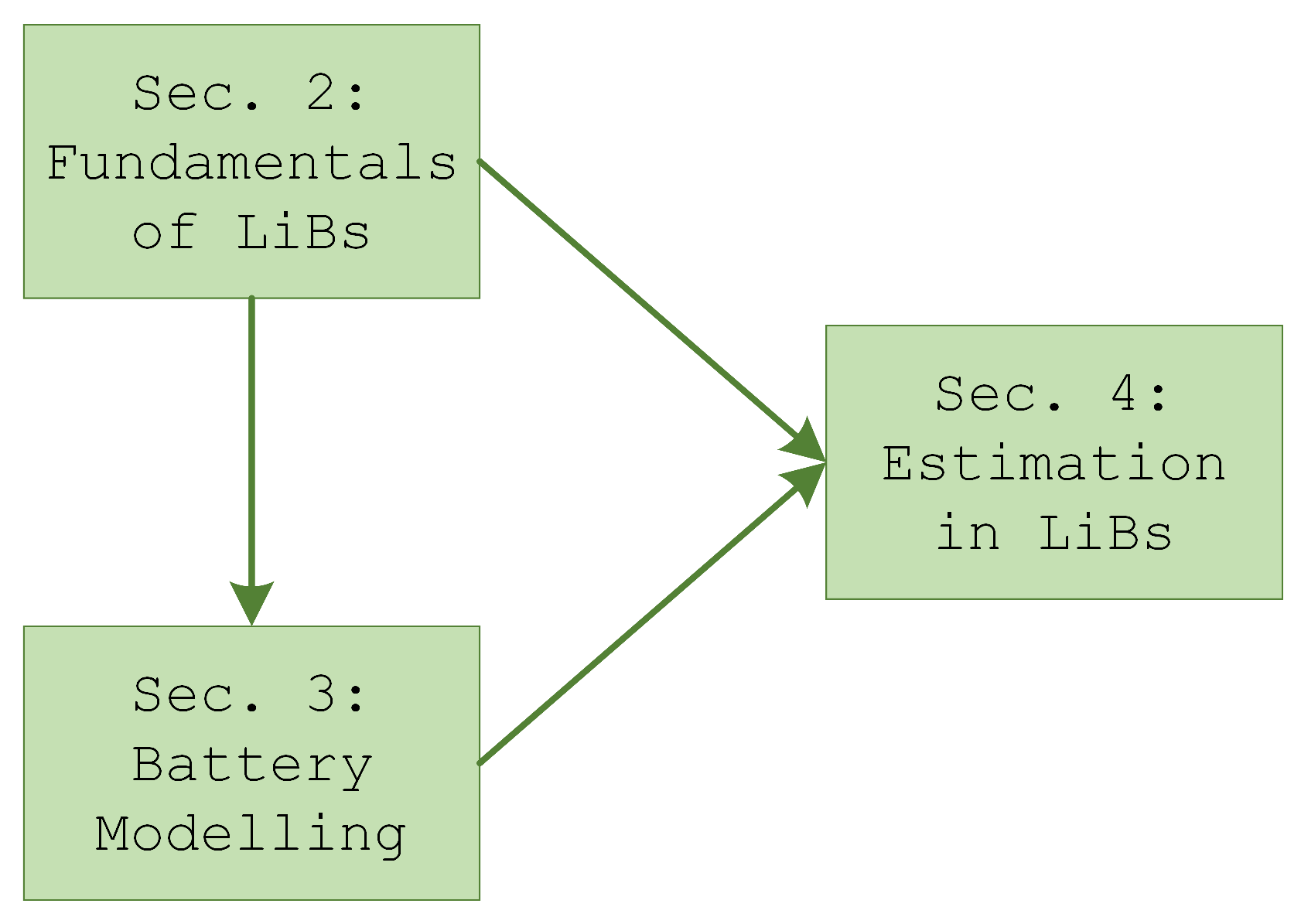
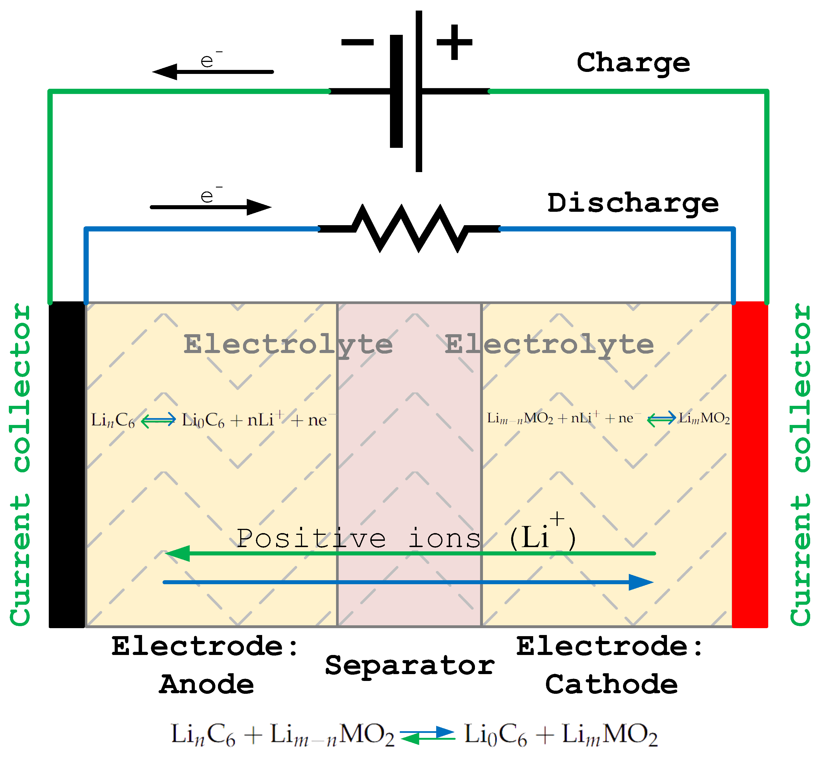
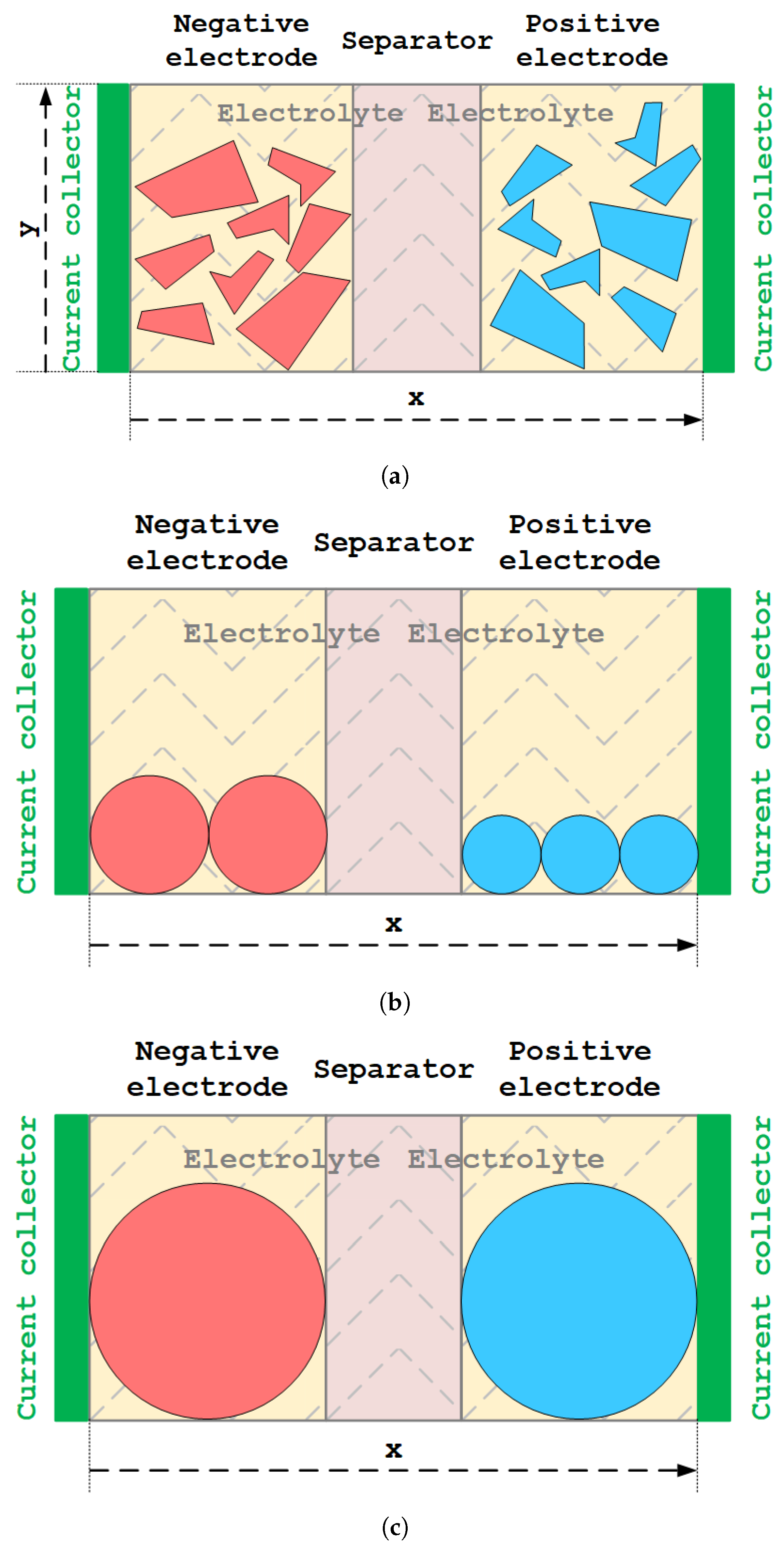
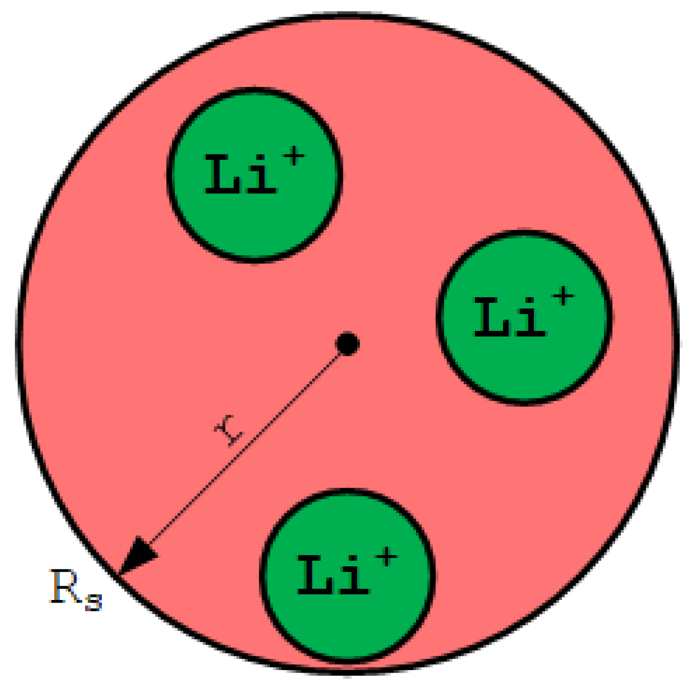
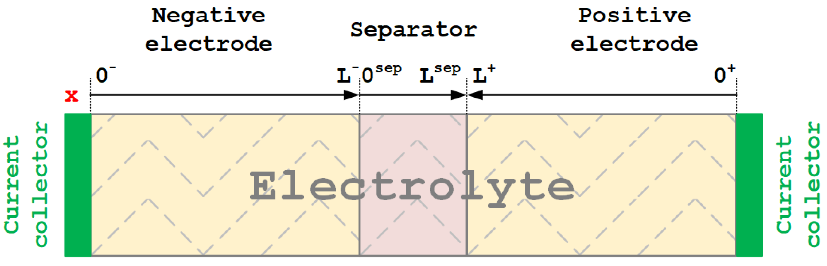
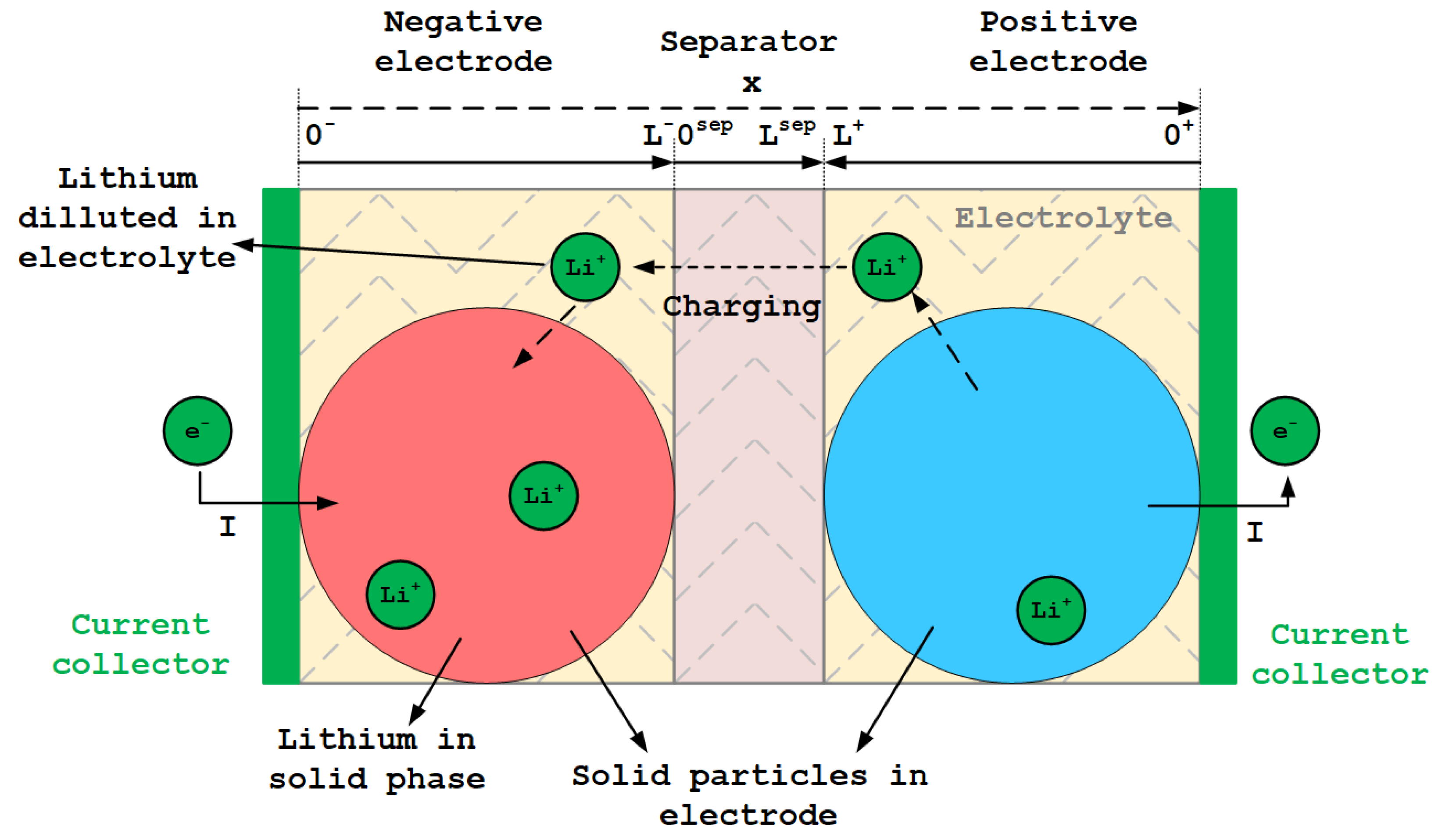
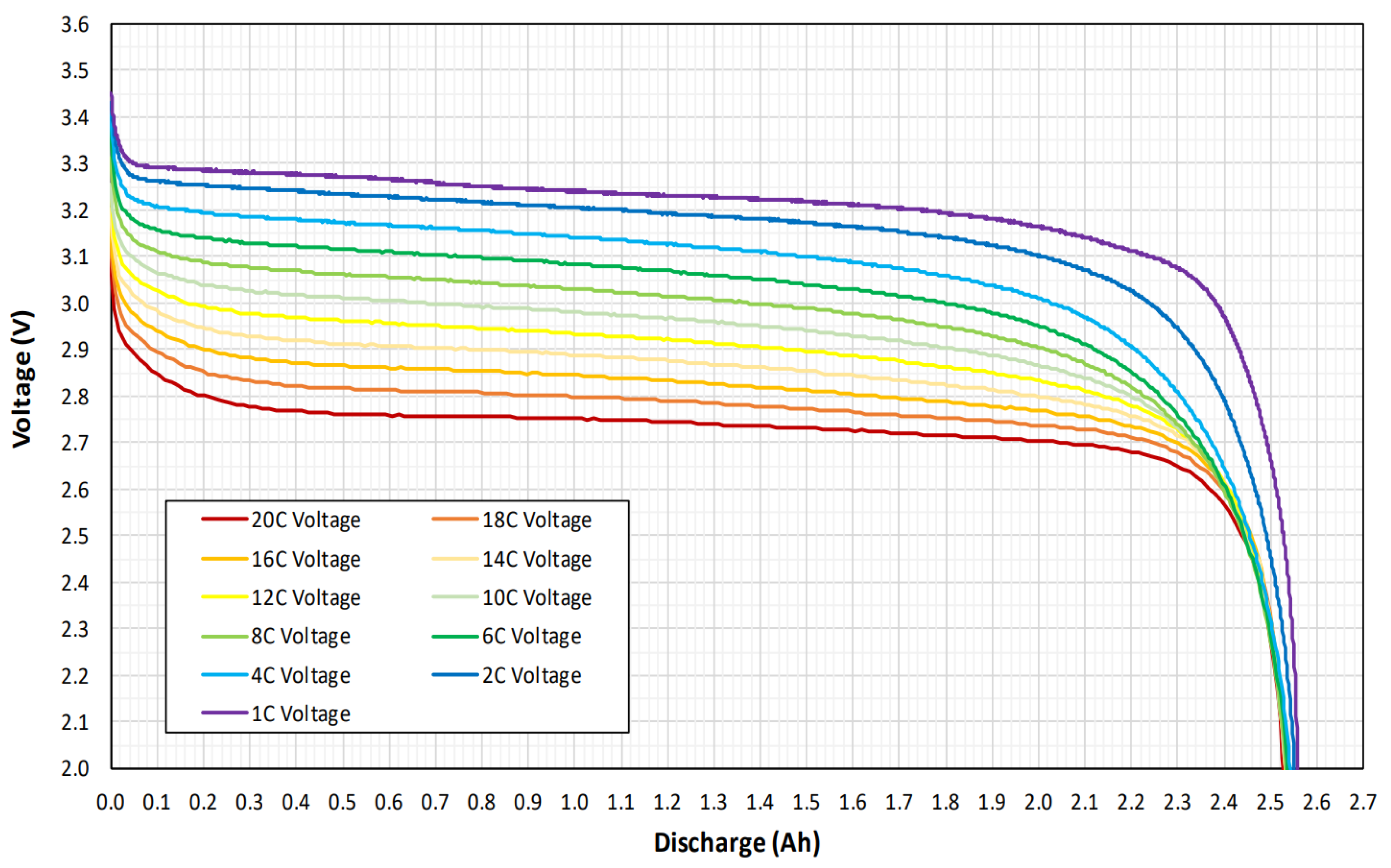
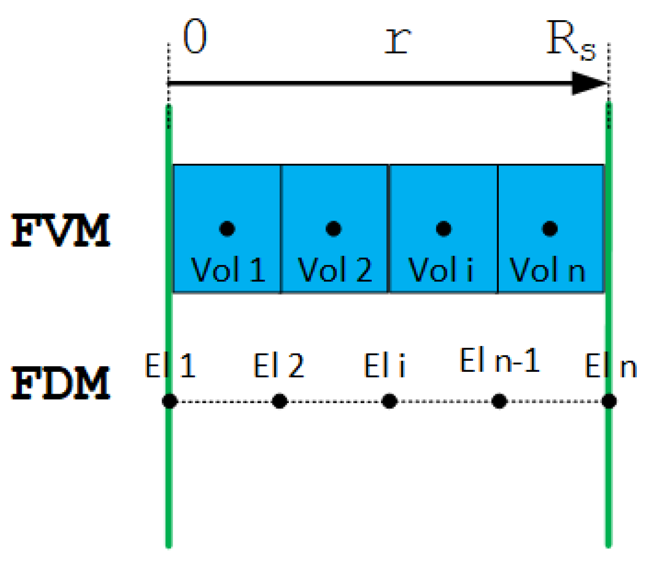
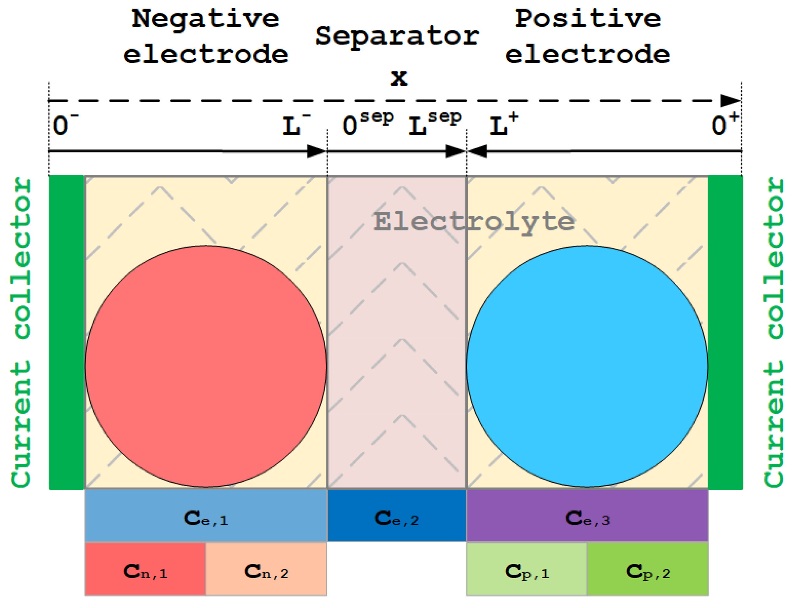
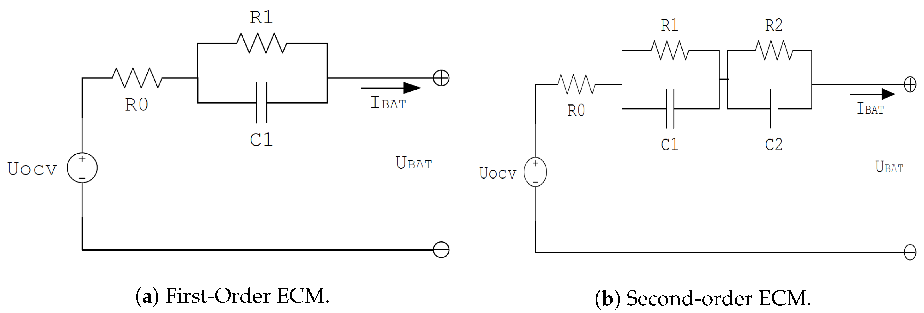
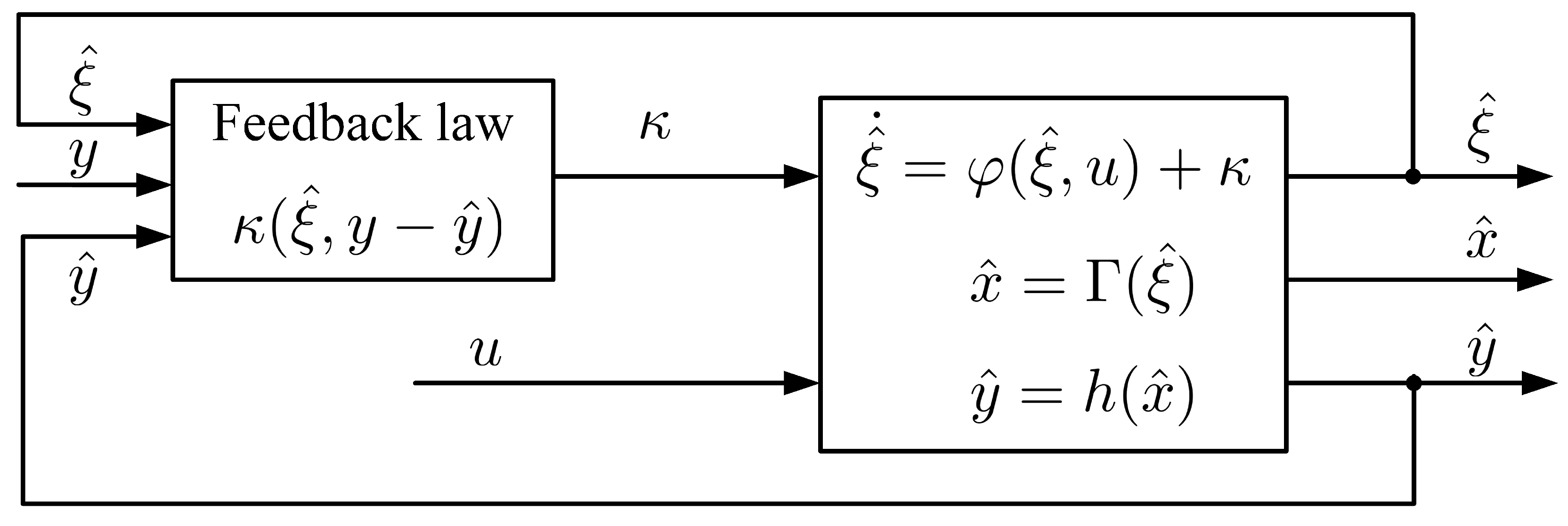
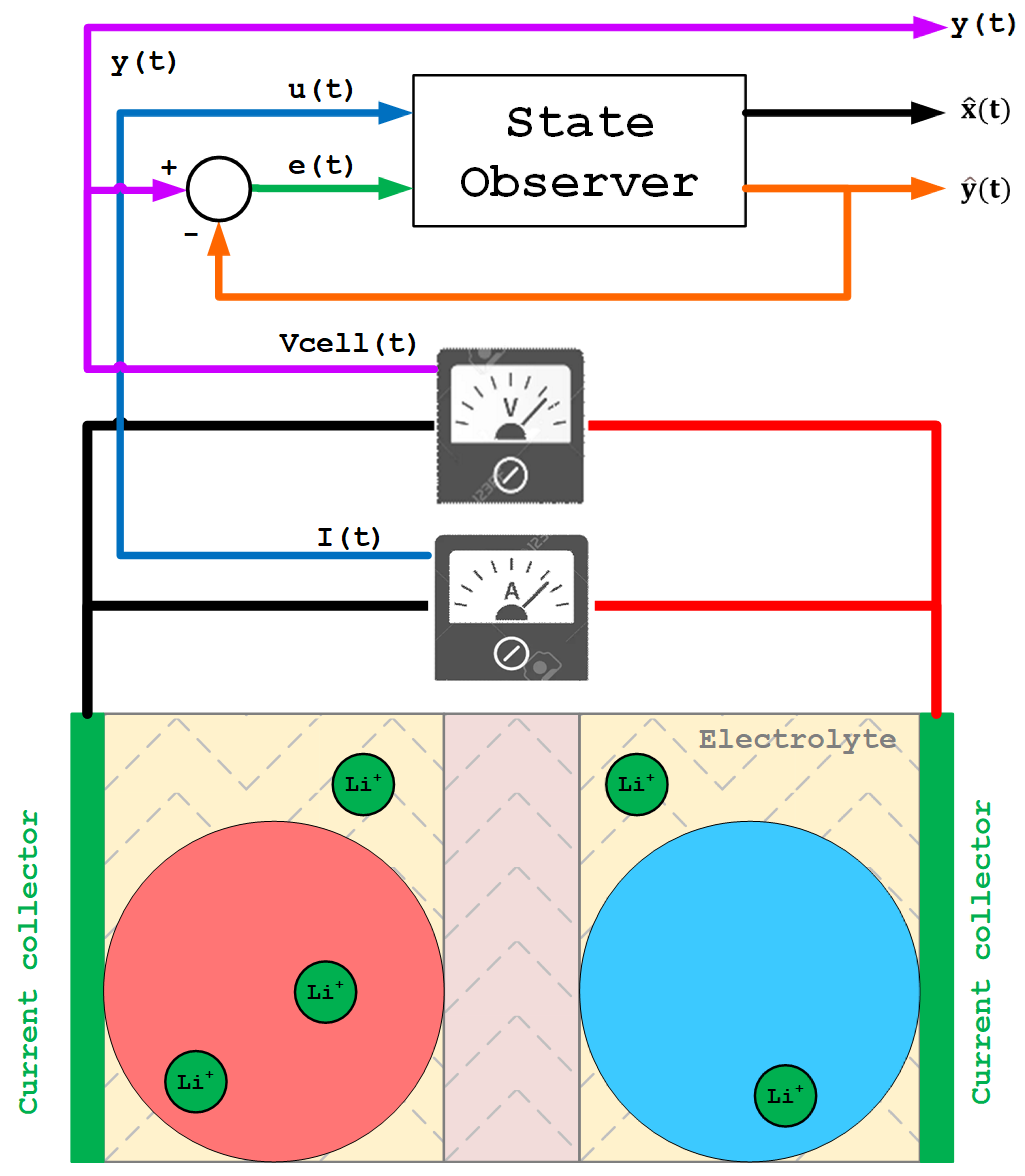
Table 1.
Side reactions by region and cause. The effects caused by overvoltage, undervoltage and high C rates in a concrete region are listed [14,21].
| Region | Overvoltage | Undervoltage | High Currents |
|---|---|---|---|
| Negative electrode | Lithium plating | Solid electrolyte interphase | Particle fracture |
| Positive electrode | Oxidation of electrolyte | Solid electrolyte interphase | - |
Table 2.
Different LIB families compared on a scale of 1–4 in terms of cost, energy (Ah), power (W), safety, lifespan and performance [10]. The highest score is 4.
Table 2.
Different LIB families compared on a scale of 1–4 in terms of cost, energy (Ah), power (W), safety, lifespan and performance [10]. The highest score is 4.
| Chemistry Family | Capacity | Specific Power | Safety | Performance | Lifespan | Cost |
|---|---|---|---|---|---|---|
| LCO | 4 | 2 | 2 | 3 | 2 | 3 |
| LMO | 3 | 3 | 3 | 2 | 2 | 3 |
| LFP | 2 | 4 | 4 | 3 | 4 | 3 |
| NMC | 4 | 3 | 3 | 3 | 3 | 3 |
| NCA | 4 | 3 | 2 | 3 | 3 | 2 |
| LTO | 2 | 3 | 4 | 4 | 4 | 1 |
Table 3.
Parameters for DFN and SPM.
| Symbol | Definition | Unit |
|---|---|---|
| Parameter/variable related to solid | - | |
| Parameter/variable related to electrolyte | - | |
| Concentration of x | ||
| Diffusion of x | ||
| r | Radial coordinate | m |
| Radius of particle x | m | |
| F | Faraday constant | |
| Electroactive surface area of x | ||
| A | Cell cross-sectional area | |
| L | Thickness | m |
| Porosity | - | |
| Volume fraction of the solid electrode material in the porous electrode | - | |
| j | Molar flux | |
| Transference number | - | |
| Current density | ||
| I | Current | A |
| Transport coefficient | - | |
| Exchange current density | ||
| Effective electrolyte conductivity |
Disclaimer/Publisher’s Note: The statements, opinions and data contained in all publications are solely those of the individual author(s) and contributor(s) and not of MDPI and/or the editor(s). MDPI and/or the editor(s) disclaim responsibility for any injury to people or property resulting from any ideas, methods, instructions or products referred to in the content. |
© 2023 by the authors. Licensee MDPI, Basel, Switzerland. This article is an open access article distributed under the terms and conditions of the Creative Commons Attribution (CC BY) license (https://creativecommons.org/licenses/by/4.0/).
Share and Cite
MDPI and ACS Style
Martí-Florences, M.; Cecilia, A.; Costa-Castelló, R. Modelling and Estimation in Lithium-Ion Batteries: A Literature Review. Energies 2023, 16, 6846. https://doi.org/10.3390/en16196846
AMA Style
Martí-Florences M, Cecilia A, Costa-Castelló R. Modelling and Estimation in Lithium-Ion Batteries: A Literature Review. Energies. 2023; 16(19):6846. https://doi.org/10.3390/en16196846
Chicago/Turabian StyleMartí-Florences, Miquel, Andreu Cecilia, and Ramon Costa-Castelló. 2023. "Modelling and Estimation in Lithium-Ion Batteries: A Literature Review" Energies 16, no. 19: 6846. https://doi.org/10.3390/en16196846
Note that from the first issue of 2016, this journal uses article numbers instead of page numbers. See further details here.