Analysis of Ice Formation during Start-Up of PEM Fuel Cells at Subzero Temperatures Using Experimental and Simulative Methods


1
Chair of Thermodynamics of Mobile Energy Conversion Systems (TME), RWTH Aachen University, Forckenbeckstraße 4, 52074 Aachen, Germany
2
The Hydrogen and Fuel Cell Center (ZBT), Carl-Benz-Straße 201, 47057 Duisburg, Germany
*
Author to whom correspondence should be addressed.
Energies 2023, 16(18), 6534; https://doi.org/10.3390/en16186534
Submission received: 14 August 2023
/
Revised: 3 September 2023
/
Accepted: 5 September 2023
/
Published: 11 September 2023
(This article belongs to the Section A5: Hydrogen Energy)
Abstract
:Freeze start is a challenge in the commercialization of PEM fuel cells. In this study, ice formation in cell layers is investigated through experiments and simulations. Segmentation of the fuel cell on the test bench allows to determine the local distributions of current density and high frequency resistance over the active cell area. The location and timing of ice formation are analyzed in the experiments. It is shown that the formation of ice lenses can be detected by local measurements of the high frequency resistances. Then, a multiphysical CFD model is built and validated with the measurements and the commonalities and differences between the model results and the experiments are studied. It is shown that the model determines the freeze start behavior very well in wide operating ranges. Together with the findings from the experimental investigations, the model will finally be used to investigate local ice formation in detail.
1. Introduction
PEM fuel cells have the potential to become a future alternative to conventional propulsion systems with internal combustion engines. Particularly in urban regions, vehicles powered by fuel cells can help to reduce pollutant emissions. However, due to its high power density, low operating temperature, and noiseless operation, a PEM fuel cell can be used not only in the vehicle sector but also in aviation and shipping [1,2].
PEM fuel cells have already left the testing and development stage due to intensified research in recent years, so increasing commercialization can be expected in the next few years [3]. For this purpose, it must be ensured already in the development phase that the cells also work reliably and efficiently in extreme situations. Frost startup in particular is also a challenge for modern fuel cell systems.
Since water is the only exhaust gas produced during operation of a PEM fuel cell, it can freeze to ice at operating temperatures below the freezing point of water. Ice lenses hinder gas transport to the catalyst layers, reducing fuel cell performance, efficiency, and lifetime [4]. As a result, frost starts without external supply of heat below −10 °C are generally not possible [5]. In addition, ice leads to mechanical stresses on the cell layers. High local mechanical stress peaks can exceed the allowable material stresses, leading to permanent damage or even destruction of the cells [6]. Thus, to understand and improve the frost start behavior, a thorough understanding of the processes in the cells during the start procedure is necessary.
Experimental research of frost starts on test benches is expensive and time-consuming. In addition to the costly purchase of the cooling units, the tests also require a great amount of time, since the cells must be carefully conditioned, dried, and frozen before each frost start procedure. Only in this way can the same initial conditions be created for each frost start test [4]. Since the highly inhomogeneously distributed processes inside the cell, such as ice formation, cannot be measured on test benches, it is essential that accompanied three-dimensional CFD simulations be performed for frost start research [7].
2. Literature Research
The increasing interest in PEM fuel cells as an alternative propulsion system has brought the frost start problem into the focus of current research. For this reason, studies by various researchers can be found in the literature that have experimentally investigated frost start processes. Most of the studies are concerned with the effects of ice formation on degradation and the associated reduction in cell performance. Others, however, also address the fundamental question of up to what starting temperature successful frost starts are still possible (cf. [5,8,9,10,11,12,13,14,15,16,17,18,19,20,21,22,23,24]).
For a better understanding of the processes taking place inside the cells during a frost start, it is useful to measure the current density or also the high frequency resistances (HFR) locally. The measurement of the current density distribution is basically possible in several ways. In all cases, the flow field on the anode or cathode side must be divided into elements of equal size that are electrically isolated from each other [25]. The current density can then be measured directly in the segments via a so-called printed circuit board (PCB), which replaces the current collector plate [26]. Alternatively, the segmented currents can be determined via electrical resistors at the segments by measuring the voltages dropping across them or with the help of Hall sensors. To do this, the resistors or Hall sensors must be mounted between the segmented flow field and the current collector plate [27,28,29]. For more information on segmented measurements on fuel cells, see the paper by Perez et al. [29]. Studies of fuel cells using the segmented measurements of current densities or HFRs can be found, for example, in [30,31,32,33,34,35].
Significantly less studies investigate frost start behavior using segmented measurements (cf. [36,37,38,39,40,41,42,43,44,45,46]).
With the help of segmented measurements, it is possible to determine the local current densities and the local HFRs and thus the local internal resistances of a PEM fuel cell during a frost start. The local distributions of liquid water or ice, for example, cannot be measured or can only be measured with extensive experimental effort. However, these can be approximated with the use of simulation.
Multidimensional and multiphysics CFD models are essential for higher accuracies, but these cannot be used for comprehensive system studies due to their high computation times [49]. To reduce computational times, only sections of flow fields can be modeled for transient frost start simulations rather than complete flow fields. Models that include a complete cell, such as the model of Fink et al., are only applicable for static simulations of individual operating points [50].
Therefore, most CFD models of fuel cells simulate only a single gas channel including the associated regions of the MEA (cf. [6,7,51,52,53,54,55,56,57,58,59,60,61,62,63,64]). Multiple parallel single channels are also conceivable (cf. [65,66,67]). Due to the aforementioned computational time constraints, fuel cell stacks cannot be modeled as a complete entity. However, Luo et al. reduce three cells of a stack to a single channel each, allowing simulation of heat transfer between individual cells in one model [68].
3. Novel Approach of This Study
The literature review shows that although there are many studies dealing with modeling of the local processes inside the cell during frost starts, these models are not extensively compared with measured data (cf. [6,54,57,60,66,69,70]) or only simple validations are carried out (cf. [53,55,58,59,62,63,64,68]). The only validations with measurements of local current densities can be found in the studies by Hakenjos et al. and Fink et al. However, these researchers only deal with static operating points and not with frost starts or other transient operations [50,71].
Since it is very important to first evaluate how accurately the models predict the measured frost start behavior, the simulation results found in literature can only be transferred to the real behavior of the cells to a limited extent. In this study, these gaps will be addressed. First, measurements of local current densities and local HFRs are performed on a segmented single cell, initially at static operating points at temperatures above the freezing point. This is followed by transient and local measurements during frost starts with different starting conditions. The developed CFD model of the cell is then compared with the measurements at temperatures above and below the freezing point. All measured conditions are subsequently simulated and the measured local current densities and the measured local HFRs are compared with the simulated values. This is followed by an evaluation of how well the model approximates the real behavior. This highlights the potential of using CFD models in researching and improving frost start behavior.
4. Theoretical Formulation
In this section, the theoretical basics of the CFD cell model are explained. The model is built in the commercial software ANSYS Fluent 2021 R2. In ANSYS Fluent, only the basic multidimensional transport equations are solved. The remaining equations describing the behavior of the modeled PEM fuel cell are included in the software via so-called User Defined Functions in C code. The fuel cell module pre-implemented in ANSYS Fluent is not used in the presented investigations. The fact that the model is built completely by the user results in a better controllability of the model.
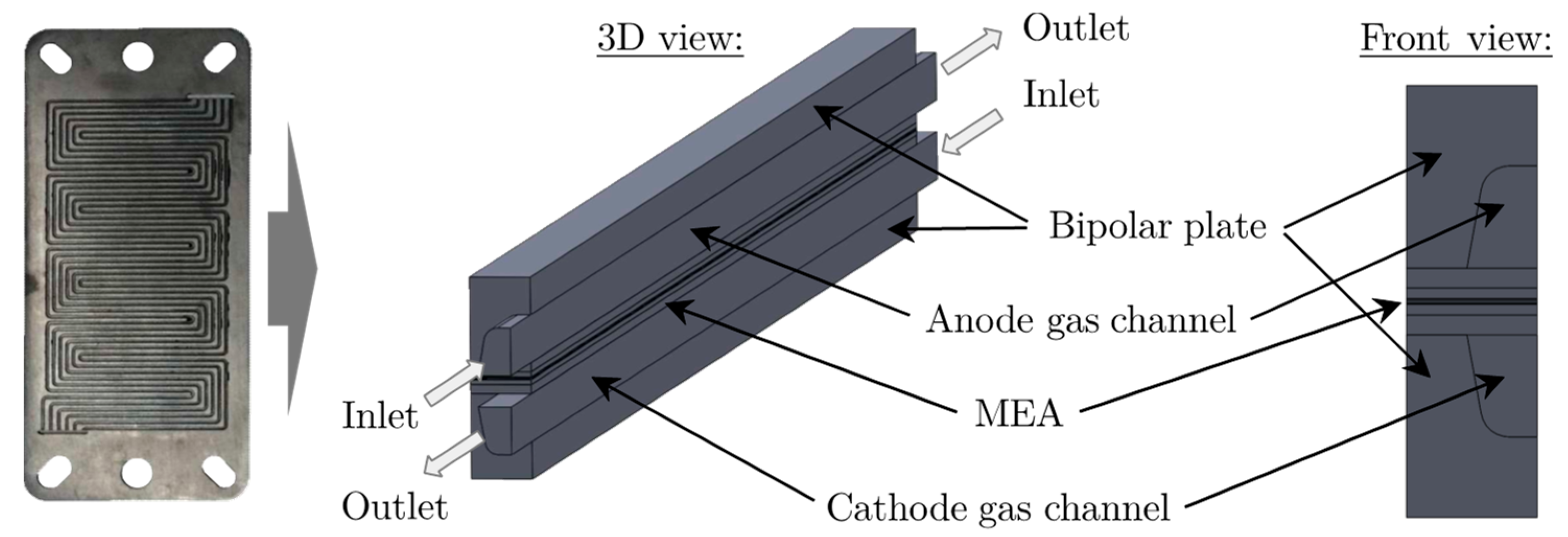
In Figure 1 (left) the flow field of the investigated cell is shown. Since the membrane and the thin diffusion layers in the cell must be very finely meshed for stable simulations, the entire cell cannot be modeled. This would increase the computational effort too much to perform transient frost start simulations. Since the flow field consists of six parallel gas channels of equal length, only one gas channel including the underlying regions of the MEA is modeled. This is a necessary simplification to be able to calculate transient frost starts in acceptable computational time. The geometry of the single-channel model derived in this way is shown in Figure 1 (right). Since the gas channels are symmetric, only one half of the channel needs to be simulated (cf. Figure 1).
The following further assumptions are made for the model setup:
- Gas mixtures obey the ideal gas law
- All gases are assumed to be incompressible
- Laminar flow due to small pressure gradients and small flow velocities
- Water exists in the aggregate states gaseous, liquid and solid and is present in dissolved form in the membrane
- Negligible gas crossover through the membrane
- Membrane consists of pure Nafion
- Convective transport of liquid water is negligible in the porous cell layers compared to transport by capillary forces
- The electrochemistry obeys the Butler-Volmer model
- The movement of ice lenses in the porous cell layers is neglected and ice is assumed to be immobile
- The gas diffusion layers are isotropic and homogeneous
- Constant temperature of the coolant over the length of the bipolar plate
In the following, the physical model equations underlying the CFD model are explained. The parameter values used are listed in Table A1 in the Appendix A. The names of the variables and their units can be found in the section Nomenclature at the end of this paper.
4.1. Modeling of the Gas Transport
The equations of mass conservation, momentum conservation and transport of gas species are taken from [72]. The pressure loss in the porous cell layers is determined by Darcy’s law from the flow velocity of the gases [72]:
Due to the porosity of the gas diffusion layers , the transport paths of the gases become longer. To take this into account in the model, the diffusion coefficients of the gases are corrected using the law of Bruggemann. At the same time, the influence of liquid water droplets in the pores on diffusion is considered:
4.2. Transport of Liquid Water
The transport of liquid water in the cell is determined by the following equation. Transport in the gas channels is purely convective, since liquid water droplets are dragged along by the gas flow. In the porous cell layers, transport is dominated by capillary forces [73].
The convective transport is considered by the factor . Since convective transport is neglected in the diffusion layers of the cell, applies there. In the gas channels, it is assumed for simplicity that the liquid water droplets move with the same velocity as the gas due to the gas flow. Consequently, is valid there [74]. The transport by capillary forces is determined by the transport coefficient .
The fraction of liquid water is defined as the volume of liquid water relative to the total fluid volume :
The transport coefficient of liquid water is determined from the liquid permeability , the viscosity of liquid water and the capillary pressure :
4.3. Modeling of Ice Formation
It is assumed that ice cannot move in the cell. Thus, the distribution of ice in the cell layers is described by the following mass conservation equation:
The ice fraction is defined as the ice volume related to the pore volume of the cell layers :
4.4. Phase Change Physics
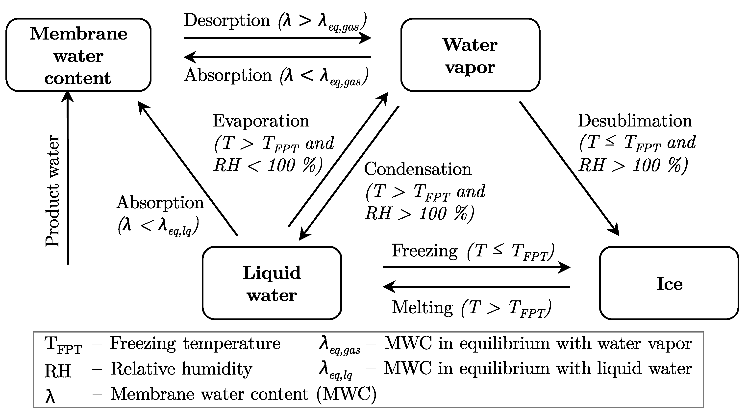
Depending on the operating temperature and pressure in the cell, water can exist in all three aggregate states. In addition, dissolved water is present in the membrane [49]. In Figure 2, the different states of water and the phase changes between each state implemented in the CFD model are shown graphically. The product water is formed in the dissolved state in the membrane fractions in the CCL. Due to the very small pore radii of the porous diffusion layers and catalyst layers, the surface tension of the water causes the freezing point to be depressed [4]. As a result, the temperature at which liquid water freezes into ice is determined by [58]:
Evaporation and condensation are determined by the difference between the saturated vapor pressure and the local partial pressure of water vapor . In addition, the temperature must be above the freezing point [55]:
Water freezes to ice if the local temperature is below the freezing point. Ice melts to liquid water if the temperatures are above the freezing point temperature [55]:
Desublimation, the direct phase change from water vapor to ice occurs when the relative humidity is greater than 100% and at the same time the temperature is below the freezing point temperature [69]:
4.5. Membrane Model
The transport of dissolved water in the membrane is modeled by the following equation [73]:
Dissolved water is mainly transported diffusively through the membrane. At the same time, when protons move from the anode through the membrane to the cathode, water molecules are dragged along. This transport is called electro-osmotic drag.
The diffusion coefficient of solved water in the membrane [77]:
Absorption and desorption of water dissolved in the membrane happens in contact with water vapor and liquid water [74]:
In contact with humid gases, sorption is determined by the difference between the local membrane water content and the theoretical membrane water content in equilibrium [74]:
The theoretical membrane water content in equilibrium is given by the following function [78]:
Absorption from liquid water into the membrane can be calculated using the difference between the local membrane water content and the theoretical membrane water content in equilibrium with liquid water () [74]:
4.6. Electro-Chemistry Model
The transport of electrons takes place in the bipolar plates, in the gas diffusion layers and in the catalyst layers. The transport of protons happens only in the ionomer (i.e., in the membrane and due to the ionomer fractions also in the catalyst layers). The transport of both charge carriers is modeled by the following equations [75]:
The transport is driven by the electric and the protonic potential , respectively.
The proton conductivity in the membrane is a function of temperature and the local membrane water content [79]:
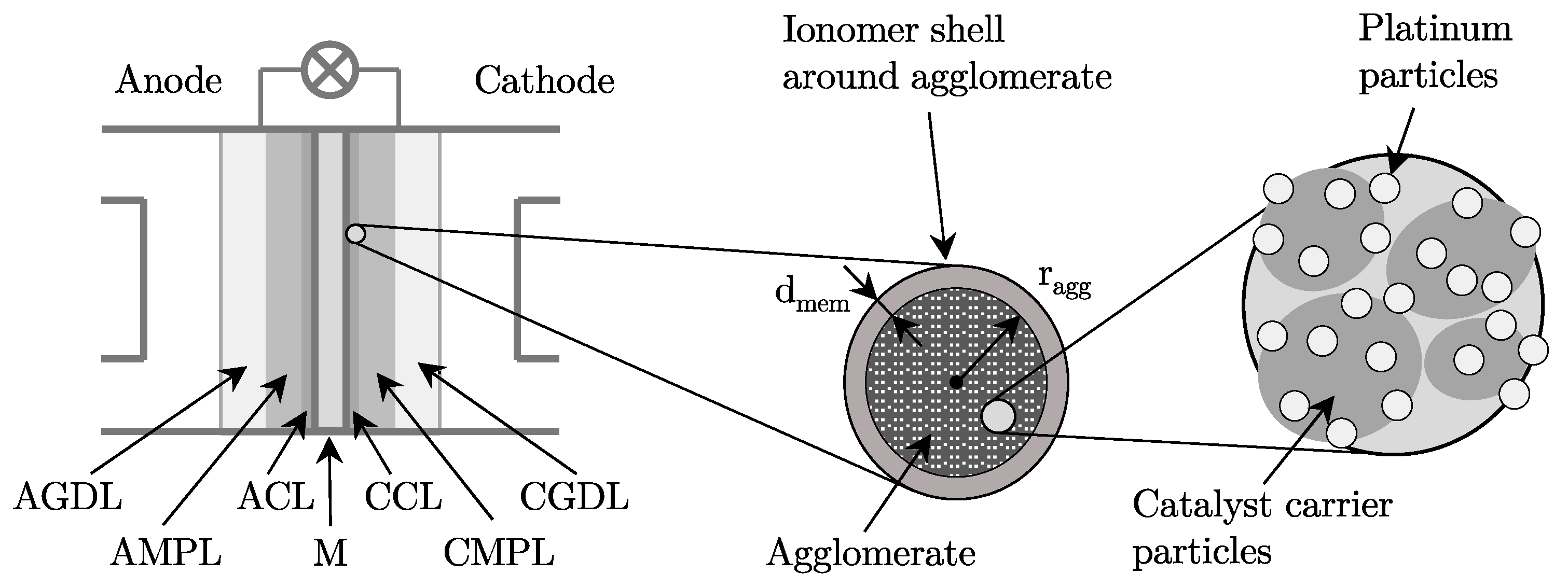
The catalyst layer of a PEM fuel cell consists of agglomerates of carbon particles, on whose surface are platinum particles and parts of the ionomer of the membrane [80]. Simplifying, the agglomerates can be modeled as spheres, on the surface of which the platinum is distributed. The agglomerates are surrounded by a uniform layer of ionomer. For the electrochemical reaction, the oxygen in the CCL must first dissolve in the ionomer shell and then diffuse through it to the platinum surface. The behavior of the fuel cell is strongly determined by these mass transfer resistances. The described structure of the agglomerate model is shown in Figure 3.
Using the agglomerate model of Sun et al., the volumetric current density of the oxygen reduction reaction (ORR) in the CCL follows to [80]:
With the local reaction rate modeled via a Butler-Volmer approach [80]:
The equation for determining the diffusion coefficient of dissolved oxygen in the ionomer is a combined equation from [82,83,84]:
with:
Since the reaction kinetics at the anode are very fast, an agglomerate model is not used in the modeling of the anode and the local reaction rate of the hydrogen oxidation reaction (HOR) is determined directly using a Butler–Volmer approach [73,82]:
The Open Circuit Voltage (OCV) is determined by the Nernst equation [73]:
5. Experimental Setup
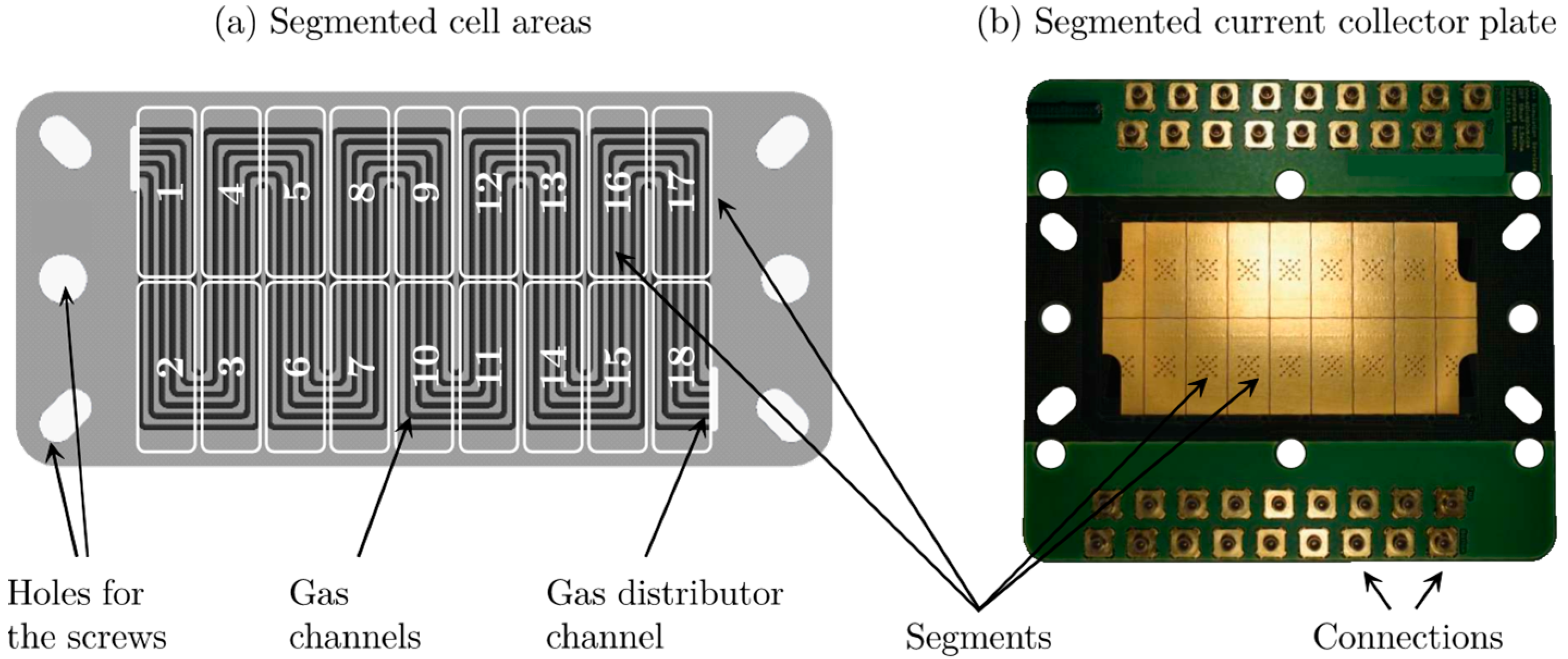
The measurements were carried out at The Hydrogen and Fuel Cell Center (ZBT) in Duisburg (Germany) as part of the research project FC COLD START: PEM-FC cold start simulations [49]. For this purpose, a single cell was used. The local current density and the local high frequency resistances of the cell are measured during the experiments. For this purpose, the active cell area is divided into 18 equally sized segments electrically isolated from each other. In each segment, the current densities and the high frequency resistances are determined using a specially made current collector plate.
In Figure 4a the current field, as well as the subdivision of the cell into the 18 segments is shown. In addition, Figure 4b shows the segmented current collector plate used to measure the local current densities and the local HFRs.
The cell on the test bench is supplied with humid hydrogen and humid air. The operating temperature is controlled by the temperature of the coolant. The temperature of the coolant can be set anywhere between −20 °C and +80 °C.
To prevent heat loss and keep the temperatures in the cell as constant as possible, the cell, end plates, and supply tubes are insulated with foam.
5.1. Steady State Measurements
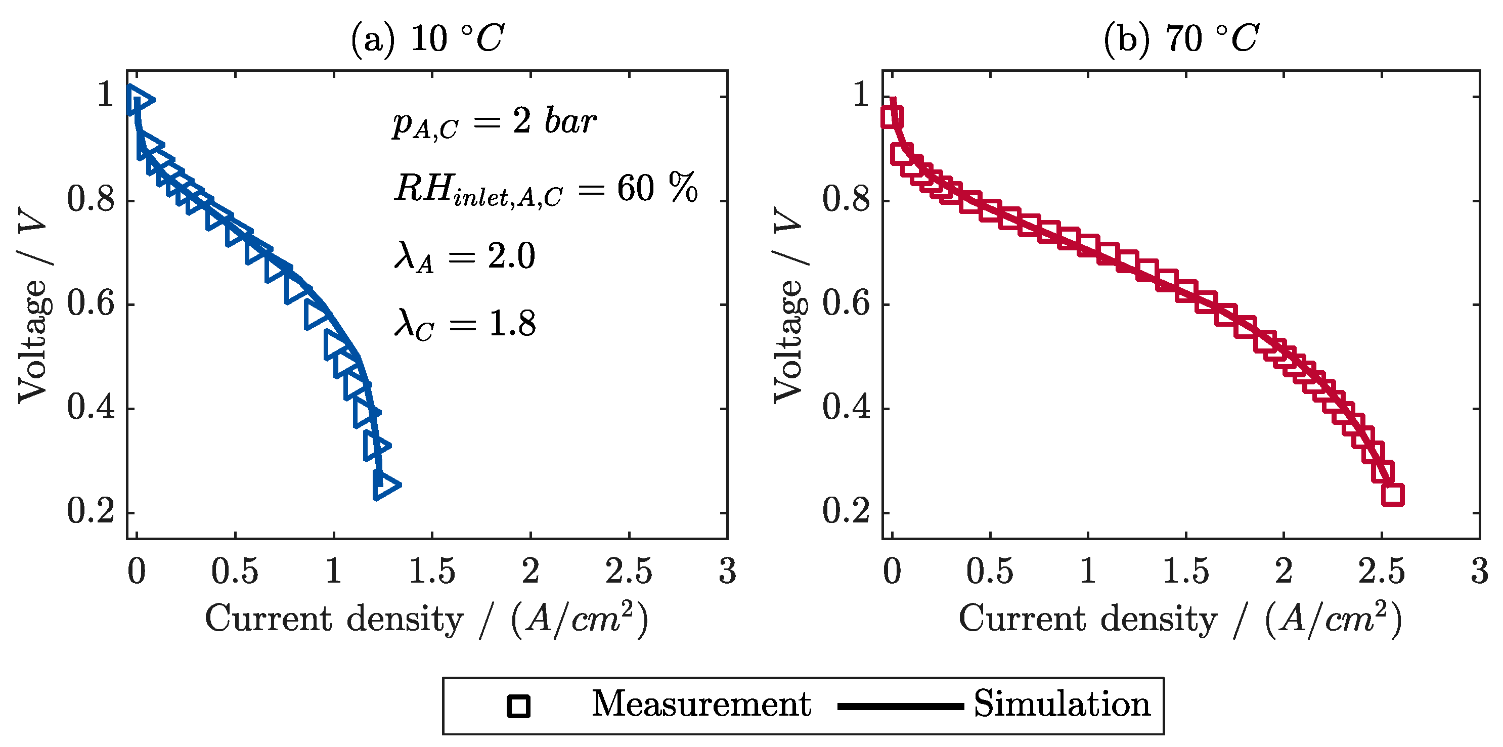
Within the scope of the investigations, the operating behavior of the cell is characterized via polarization curves. For this purpose, steady-state measurements are performed at different operating temperatures. For all measurements, the hydrogen and air entering the cell are humidified to a relative humidity of 60%.
After the cell is controlled to the desired operating temperature via the coolant, potentiostatic operation of the cell at 0.3 V for about 30 s is performed. This reduces platinum oxides. For conditioning and establishing constant conditions prior to each measurement, operation is then performed at 0.6 V for 30 min. The polarization curve is then measured in galvanostatic operation. For this purpose, the current density is first gradually increased and then gradually decreased after the limiting current density of 0.3 V is reached. Finally, for the polarization curves, the measured cell voltages are averaged for the same current densities from both increasing and decreasing operation.
5.2. Transient Frost Start Measurements
Before the actual measurements of frost start processes can be carried out, the cells must first be conditioned to a reference condition in order to create the same conditions for each start process. This ensures, for example, that the amount of liquid water in the cell is the same before each measurement. To do this, the cell is first operated galvanostatically at a constant current density of 0.8 A cm−2 for 60 min. In the subsequent step, the cell is dried with nitrogen, thereby removing the residual water. The nitrogen has a constant humidity of 25% for this purpose and is controlled to a temperature of 60 °C. After drying, the freezing phase takes place. For this purpose, the cell is conditioned via the coolant to the desired start temperature of the subsequent frost start.
The single cell has a very high thermal mass with the end plates and the measurement setup in the test bench. Therefore, the heat dissipated during operation of the cell is not sufficient to enable self-starting at temperatures below the freezing point. In order to be able to carry out frost start tests, the temperature of the cell is adjusted via the coolant. For this purpose, the temperature is increased linearly over time starting from the start temperature up to the operating temperature. The temperature increase occurs at a maximum rate of 3.6 K/min. All frost starts are performed at a constant cell voltage of 0.6 V. Hydrogen and air are supplied dry to the cell during this process.
6. Results and Discussion
6.1. Model Validation with Steady Measurements
The model is calibrated so that the simulated polarization curves match the measured ones as closely as possible at all operating temperatures. For this purpose, the values of some parameters, which are not precisely known for the fuel cell, must be adjusted. Four parameter values are adjusted for calibration, which are shown in Table 3.
A comparison between simulated and measured polarization curves is given in Figure 5. It shows very good agreement between the calculated and measured values for all operating temperatures and for all current densities studied.
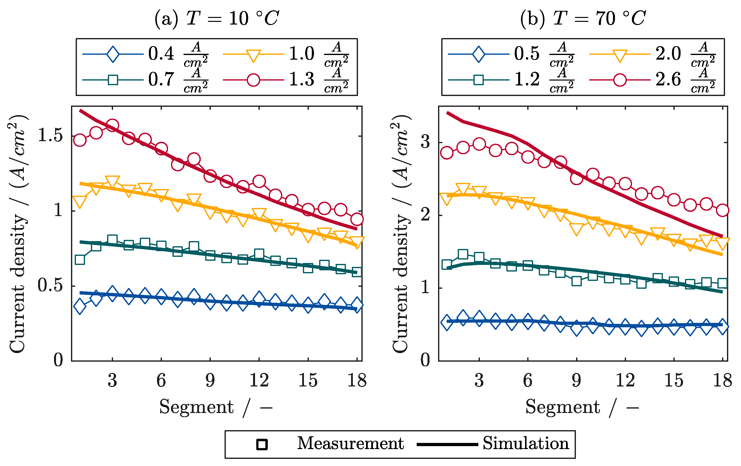
For the same operating temperatures, Figure 6 shows comparisons between the measured and simulated local current densities across the individual segments. If the cathode side is considered, segment 1 is at the inlet of the gas channel and segment 18 is at the end of the gas channel.
It is noticeable that at an operating temperature of 10 °C, the measured and simulated current densities in the segments agree very well for all current densities. Very good agreement is also obtained at higher operating temperatures for small and medium current densities.
At 70 °C and a current density of 2.6 A cm−2, the simulated current densities in the first segments are larger than the measured values. Conversely, the simulated current densities in the last segments are smaller, since in sum the same total current density is produced. Since the local current densities are significantly dependent on the local oxygen concentrations, the deviations suggest that the oxygen concentrations in the first segments of the cell on the test bench are smaller than calculated in the model. As a result, the model determines the current densities in the first segments to be too large. This indicates a requirement for further research in order to be able to determine oxygen concentrations more accurately in the future, even at very high diffusive mass flows at high temperatures. Since in this study the behavior of the cells is simulated only at low temperatures, the physics used are good enough since excellent agreements are obtained at low temperatures.
6.2. Model Validation with Transient Measurements
To enable a direct comparison between the measured frost starts on the test bench and the simulated start processes, the boundary conditions of the CFD model must be defined in such a way that they correspond as closely as possible to the specifications on the test bench. Therefore, the temperature of the coolant is also specified in the simulations and increased at a constant rate.
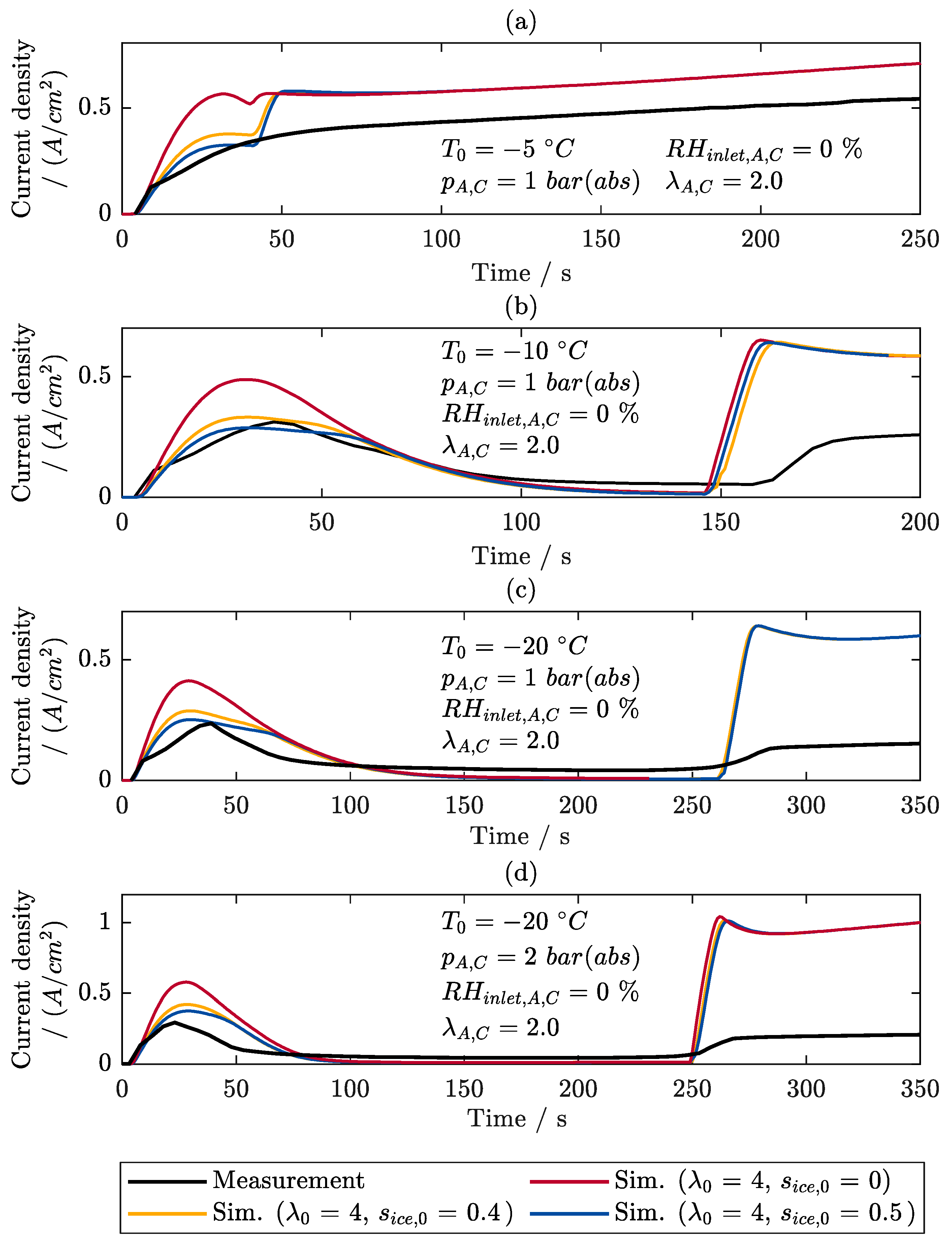
In Figure 7 a comparison between the simulated and the measured current densities of frost starts at different start temperatures and pressures is shown. All frost starts are performed potentiostatically at a cell voltage of 0.6 V. The black curves in the plots show the measured current densities.
At T0 = −10 °C (cf. Figure 7b), the current density initially increases after the beginning of the startup process, but decreases again about 40 s after the startup process begins, as ice forms in the cell. Once the temperature of the cell exceeds the freezing point temperature, the current density becomes larger again and the cell starts successfully. The same behavior can be observed at T0 = −20 °C and other pressures (cf. Figure 7c,d).
Although the temperature of the cell is initially below the freezing point of water at a starting temperature of −5 °C, the measured current density continuously increases during the starting process. No decrease in current density due to ice formation is observed (cf. Figure 7a). Due to the small pore sizes in the gas diffusion layers and the catalyst layers, the freezing point of water is shifted to smaller temperatures below 0 °C. The freezing point depression, together with the rapid temperature increase due to the heat of reaction, ensures that at a starting temperature of −5 °C, the product water cannot freeze to ice and the production of electricity is not hindered.
Assuming that no ice was formed in the cells at the beginning of the startup processes, the red curves in Figure 7 represent the simulated current density. At a starting temperature of T0 = −5 °C, the simulated current density also increases continuously. However, the simulated current density is always about 0.15 A cm−2 larger than the measured current density. Even at the starting temperatures −10 °C and −20 °C, the simulated current density increases at the beginning of the starting process and eventually decreases again due to ice formation. After the ice melts, the current density increases again. Even at this starting temperature, if no ice is present, the current density is simulated to be much larger than measured.
After drying and purging with nitrogen and before freezing, the disassembly of the cell shows that drops of residual liquid water remain in the cell layers and gas channels despite drying. Since the residual water turns to ice during freezing, the assumption that there is no ice in the cells at the beginning of frost start is not adequate. Unfortunately, the precise amount of residual water in the cells cannot be determined experimentally using the available resources. For this reason, an estimation of the amount of residual water and thus the amount of ice produced during freezing is attempted with the help of the CFD model. For this purpose, the freeze start process is simulated with the CFD model at different assumed initial ice fractions and then it is checked for which assumed ice fractions the measured and the simulated current densities correspond best. For this reason, the yellow and blue curves show the simulated current densities assuming that ice fractions of sice = 0.4 and sice = 0.5 are contained in the cells at the beginning of the startup processes.
For example, in Figure 7b, it is clear that, as a result, the simulations agree very well with the measurements (especially in the temperature range below the freezing point). The ice fraction, which is already formed from the residual water when the cell freezes, consequently has a great influence on the start process and must be taken into account in the simulations.
After the ice has melted, however, the current densities continue to be simulated significantly larger than measured. These deviations are caused by the distribution of liquid water in the cells. Melting of the ice creates a lot of liquid water in the catalyst layers. However, it is very difficult to model the effect of liquid water on the diffusion of gases through the cell layers and on cell chemistry.
This effect will be addressed in more detail in a future study, when the startup behavior of the cell after exceeding the freezing point temperature will be considered in more depth. Since only the frost start behavior at temperatures below 273.15 K is studied in the current study, this improvement is not yet necessary. The comparisons show that the model determines the behavior at very low temperatures very well. The model is therefore well suited for further investigations.
6.2.1. Segmented Current Densities during Frost Start
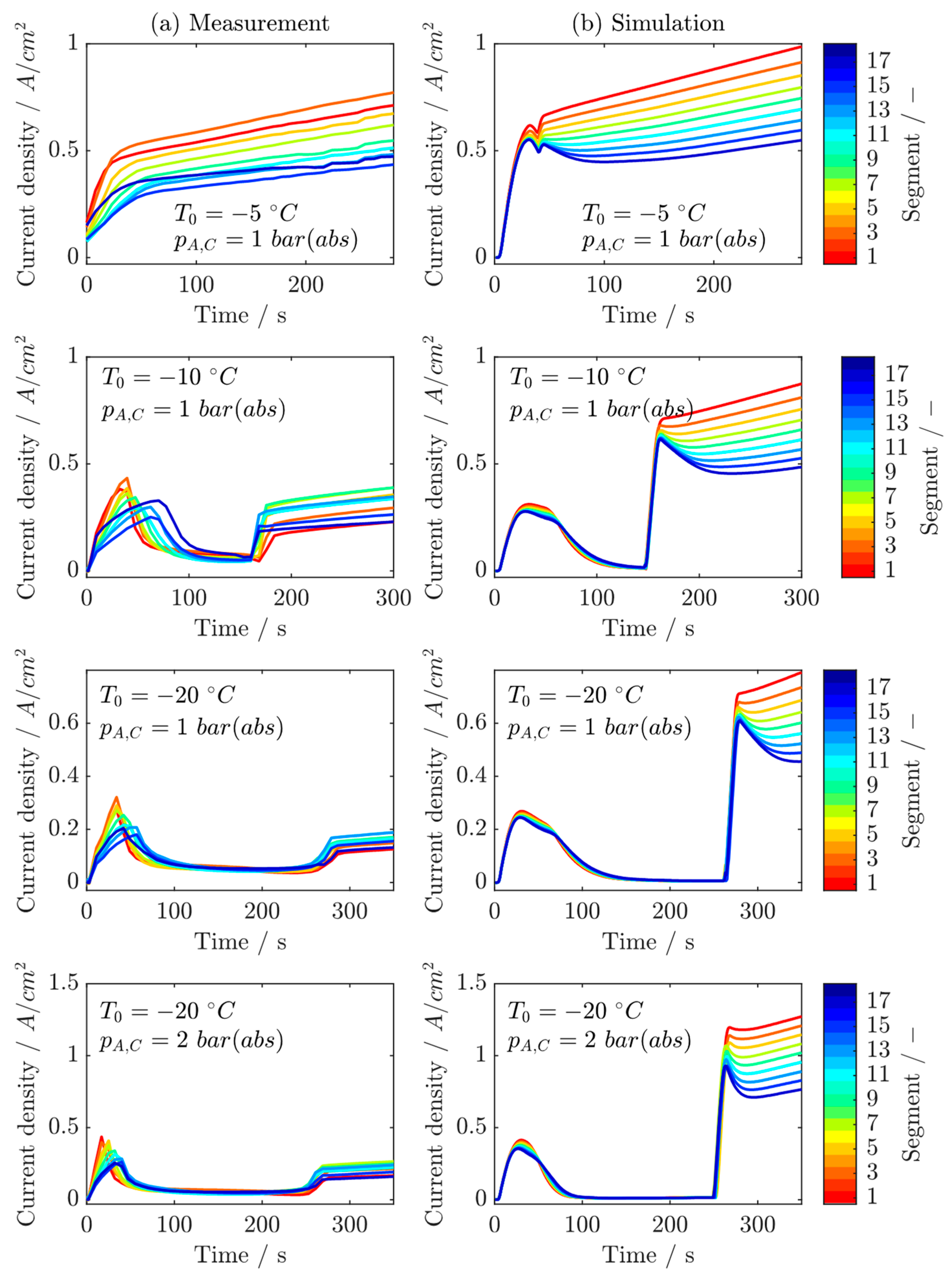
The local current densities in the 18 segments during the frost start processes which are shown in Figure 7, are visualized in Figure 8. The left subplots show the measured and the right subplots the simulated local current densities.
The measured current densities indicate that at the beginning of the frost starts, the highest current densities are generated in the front segments due to the high oxygen concentrations.
Since most of the product water is thus also generated in the front segments, the largest amounts of ice form there. The ice hinders the electrochemical reactions and the current densities become smaller. As a result, less oxygen is converted in the front segments than before and the oxygen fractions in the rear segments become larger. Thus, the current density in the rear segments increases. Since the current densities in the front segments become smaller due to the ice and increase in the rear segments due to the higher oxygen contents, there is a point in time at which the local current densities in the rear segments become larger than in the front segments.
The same behavior is calculated by the CFD model. At the beginning of the frost start, before ice is formatted, the highest current density is produced in the front segments. However, it is notable that this influence is significantly smaller than in the measurements. The differences can be attributed to the locally different temperatures in the cell. The electrochemical reactions generate heat which locally heats up the cell. Due to the higher reaction heat caused by higher local current densities, the front segments of the cell are heated up more in the first seconds of the frost starts. At the same time, the coolant in the bipolar plates in the experiment flows in the opposite direction to the flow of air through the cathode. This means that the coolant flows from the “rear” to the “front” segments, so to speak. Since the coolant continuously heats up in the cell, the coolant is therefore already preheated when it reaches the front segments. Both effects therefore create a large temperature gradient in the cell, from the front segments to the rear segments. Since higher temperatures can also generate greater current densities locally, which in turn provide more heat of reaction, this effect itself becomes more and more pronounced in the experiments. The flow of the coolant is not modeled in the model, but it is assumed that the temperature of the coolant is constant over the entire surface of the bipolar plate. Consequently, the described effect does not occur. This explains why the measured local current densities differ more than the simulated local current densities over the segments. During the formation of ice, this effect is not so strong, since it is weakened by the reduction of the local current density by the ice. Therefore, good agreements between the simulations and the measurements during the ice formation phase are shown again (cf. Figure 8b).
After the ice is melted, the measurements show that the largest current densities are now produced in the middle segments and the current densities in the front and rear segments are significantly smaller. This can also be attributed to the influence of the liquid water. Since the largest ice fractions are reached in the front segments during operation below the freezing point, the largest amounts of liquid water are also produced there after melting. The liquid water impedes the electrochemical reaction and thus ensures smaller current densities. In the rear segments, only small current densities can also be achieved due to the low oxygen content, so that the largest current densities are generated in the middle segments.
As already discussed, the comparison with the simulation results shows further demand for research, since the model is not yet able to perfectly determine the influence of liquid water on electricity production at high temperatures. The large amounts of liquid water due to melting must be transported by capillary transport to the surface of the gas diffusion layers so that they can be transported from there by the gas flow through the gas channels out of the cell. Capillary transport is slow, however, so that removal of the liquid water takes some time. This is the case both in the experiments and in the simulations. However, since the model describing the influence of liquid water on electrochemistry needs to be further improved, the local current densities after melting of the ice are simulated to be larger than measured.
However, in the context of this study, only the frost start behavior at temperatures below the freezing point is considered. Therefore, the comparison of the simulated and measured local current densities also shows that the model simulates the behavior at very low temperatures well and is very suitable for further investigations.
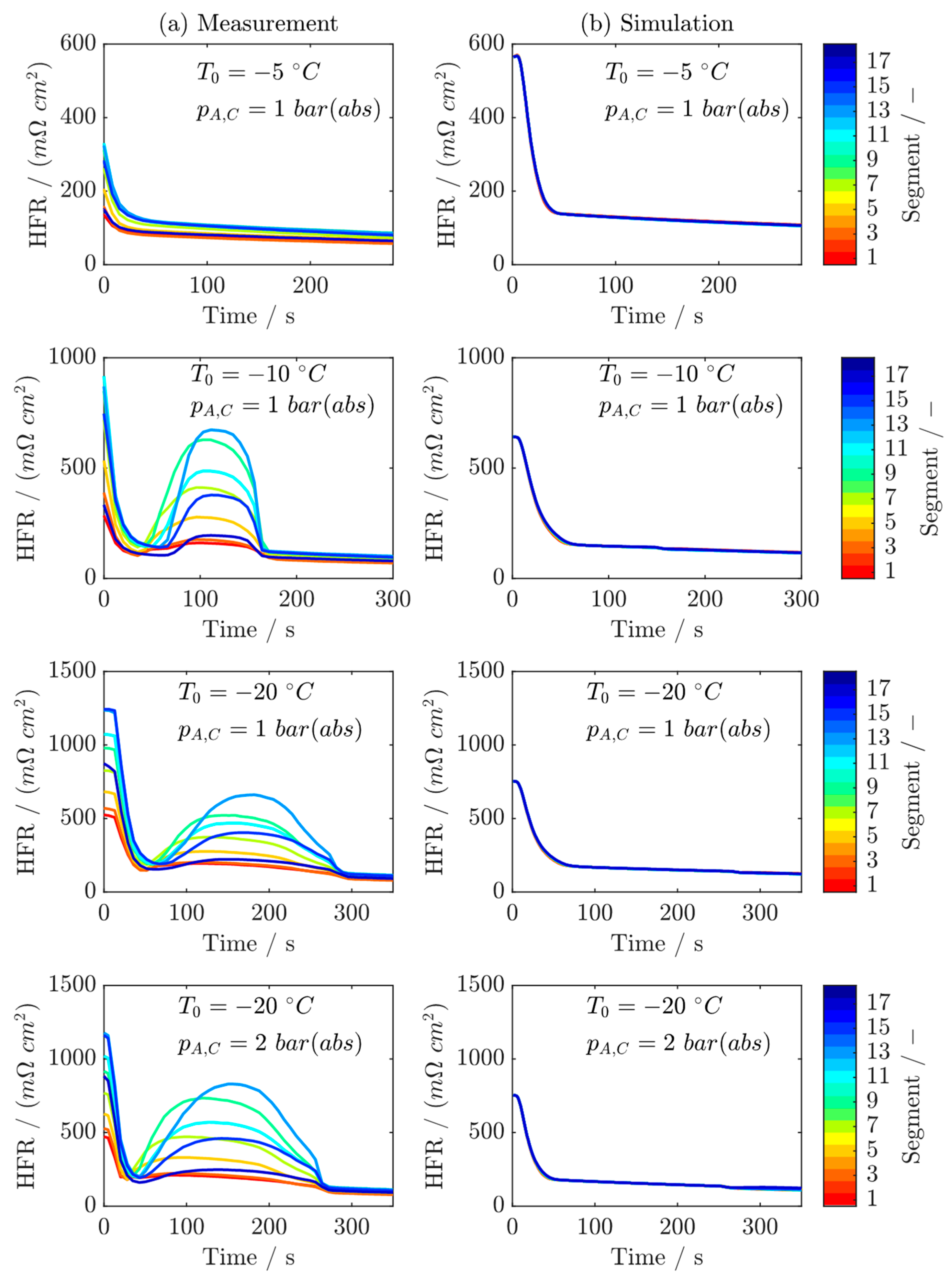
6.2.2. Segmented High Frequency Resistances during Frost Start
The local measurements of the high frequency resistances during the studied frost starts are shown in the left subplots in Figure 9. The corresponding simulated HFRs can be found in the right subplots of the same figure.
For all of the start temperatures and pressures studied, the local HFRs are high at the beginning of the start processes since the membrane water contents are low due to the previous drying phases. The local differences in the values of the HFRs in the individual segments can be attributed to the inhomogeneous distributions of the membrane water contents after drying and the uneven distributions of the contact pressures over the active cell surface due to the clamping system.
After the start-up processes begin, the HFRs initially decrease rapidly as the product water humidifies the membrane, causing the proton conductivities to increase.
At the starting temperatures of −10 °C and −20 °C, the local HFRs in the middle segments of the cell become larger during the formation phase of ice. The comparison with Figure 7 and Figure 8 indicates that this increase occurs in parallel with the decrease in current density due to ice formation. The product water causes ice lenses to form between the cell layers, resulting in local delaminations. The delaminations increase the contact resistances. As a result, the HFRs become locally larger. Due to the clamping at the edges of the cell, the cell is more elastic in the center of the active cell area than at the edges. This allows ice lenses to delaminate the cell layers more easily in the middle segments than in the front and back segments of the cell, where the large contact pressures suppress the delaminations well. Since no ice is formed at a starting temperature of −5 °C, the increase in local HFRs in the middle segments is not observed in this experiment. So, measuring the HFR is a way to be able to determine on board in a vehicle the ice formation during the frost start.
The simulated local HFRs are determined from the local membrane water contents and the membrane thickness:
In general, the local HFRs depend on many different influences besides the local proton conductivity of the membrane. In addition to the electrical conductivity of the cell layers and the bipolar plates, the cables and the connectors connecting the cell to the measurement devices also influence the measurements of the HFRs. As a result of these many unknown variables that cannot be simulated, a direct comparison between the measured and simulated HFRs is very difficult. Therefore, in this study, the simulated HFRs are determined only from the proton conductivity of the membrane. Therefore, smaller deviations are not unexpected. Qualitatively, however, a good comparison can be made between the simulated and the measured values. The simulated local HFRs during the studied frost starts are shown in Figure 9b. Due to the initial dry membranes, the simulated HFRs are also high at the beginning of the startup processes and become smaller due to the product water during operation. However, in the CFD model of the cell, the influence of the contact pressure on the contact resistances is not modeled. Therefore, the increase of the local HFRs in the middle segments of the cell cannot be observed in the curves of the simulated local HFRs.
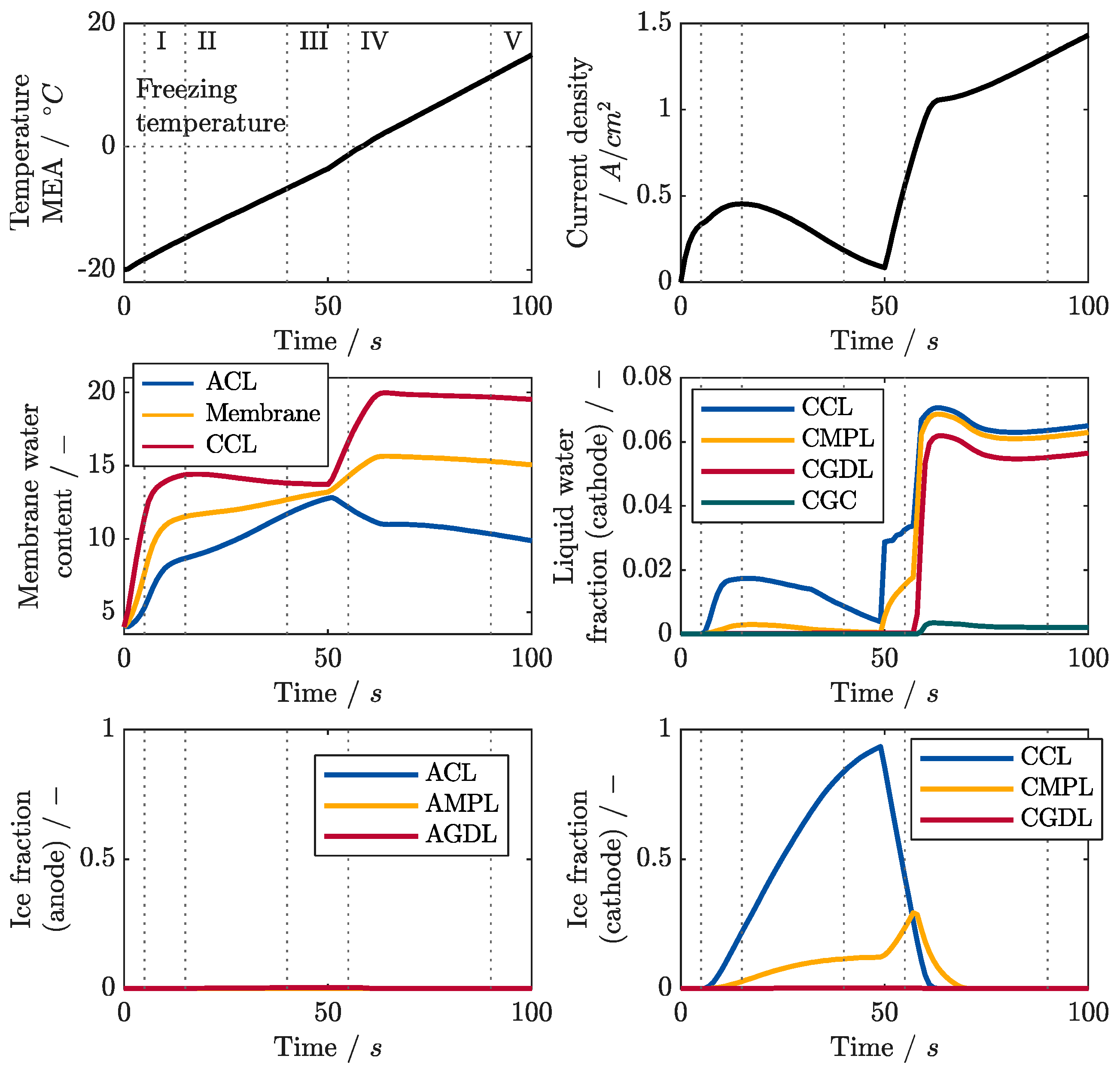
6.3. Locally Resolved Analysis of the Frost Start Process
In Figure 10, the results of a simulated frost start starting from a starting temperature of −20 °C are shown. The temperature of the coolant is increased at a rate of 1/3 K s−1 for this purpose. The figure shows the average temperature of the MEA, the current density produced, the average membrane water contents in the catalyst layers and the membrane, the average liquid water contents in the cell layers of the cathode, and the average ice contents in the cell layers and gas channels of the cell during the startup process. It is found that only ice is formed on the cathode side during frost start. No supercooled liquid water is generated on the anode side at temperatures below the freezing point, so no ice is formed either.
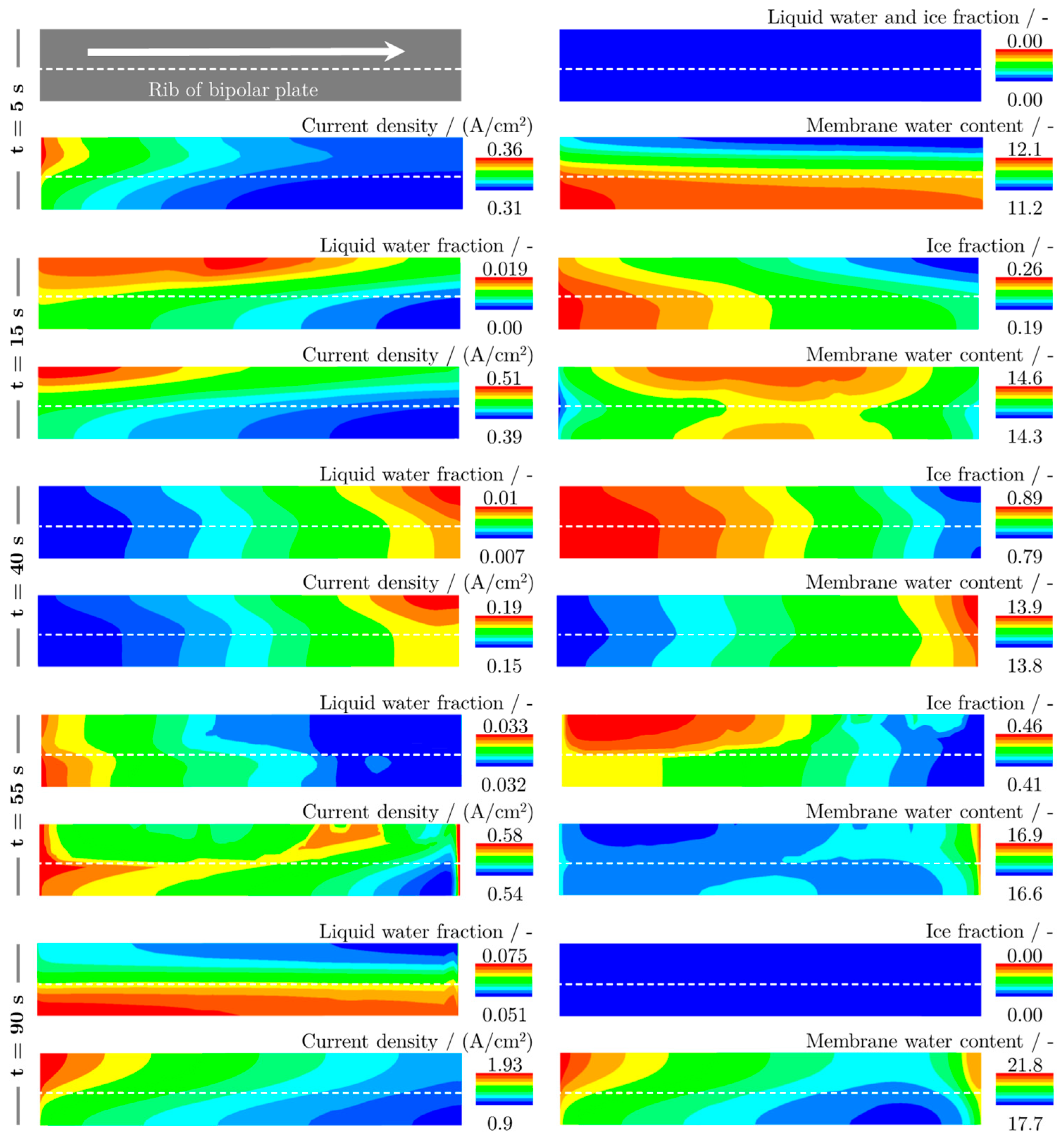
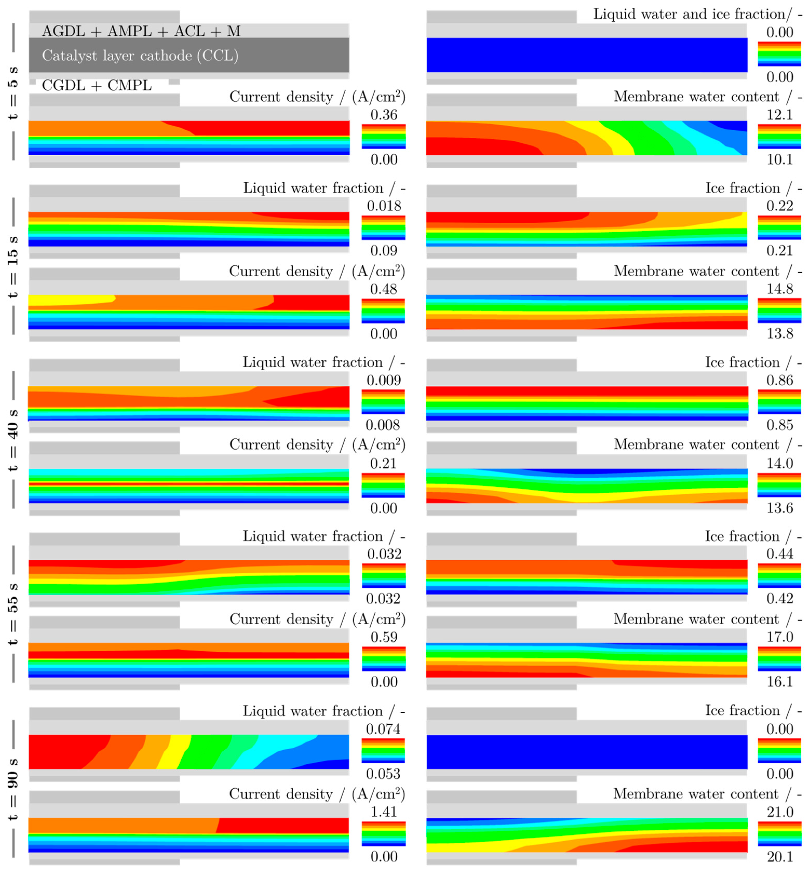
Figure 11 represents in a longitudinal section through the catalyst layer of the cathode the liquid water content, the ice content, the current density and the membrane water content during the frost start considered. The direction of flow through the cathode is indicated by the arrow. The area under the ribs of the bipolar plates is marked by a dashed line. In addition to this, in Figure 12 the values are shown in a cross section through the CCL. The positions of the ribs of the bipolar plates are marked by areas highlighted in gray.
At time tI = 5 s, the membrane is not saturated at any point, so the product water does not leave the membrane and move into the CCL. Consequently, liquid water and ice do not yet exist (Figure 11). The current density is highest at the beginning of the gas channel, since the highest oxygen contents are present there. This can also be seen from Figure 11. Along the gas channel and below the ribs, the current density becomes smaller due to the lower oxygen content, as the ribs of the bipolar plates provide longer diffusion paths from the gas channels into the catalyst layers. Figure 12 indicates from the cross-section through the CCL that the highest current densities in the CCL are generated on the side towards the membrane. This happens due to the greater proton density near the membrane. As a result of the product water being generated in the membrane, the membrane water content increases most in the areas where the highest current densities are produced. At the same time, some of the water desorbs from the membrane because the gases in the gas channels have very small relative humidities. Desorption is impeded under the ribs of the bipolar plates, so that eventually the highest membrane water contents occur in the regions under the ribs. Looking across the thickness of the CCL, the membrane water contents are smaller on the side towards the membrane than towards the diffusion layers. This occurs because the highest current densities are generated in the area close to the membrane and, due to the heat of reaction, higher temperatures are locally present there than in the area close to the ribs through which cooling is performed.
Under the rib at the beginning of the gas channel, saturation is first obtained in the membrane, so that the desorption of liquid supercooled water starts there and thus the formation of ice [7]. From time tII = 15 s, the membrane is then saturated in the complete cell, so that all of the product water enters the cell in liquid form and freezes (Figure 11). The ice fraction increases most rapidly under the rib of the bipolar plate because temperatures are lowest there. At the same time, this causes the highest amounts of liquid water to accumulate in the regions under the channel where the current density is maximum. The channel shown in Figure 12 clearly shows that the fractions of liquid water and ice are highest near the membrane, because more product water is formed there due to the higher current density.
Figure 11 illustrates that tIII = 40 s after the start of the frost start, the ice fraction in the front regions of the cell has increased so much that the highest current densities are now generated in the rear regions of the cell. Due to the product water, the largest fractions of liquid and supercooled water are now also in the rear regions under the channel. The cross-section through the CCL shown in Figure 12 illustrates that the pores near the membrane are almost completely filled with ice at this point. As a result, the highest current density viewed across the cross section is no longer generated near the membrane, but now in a small area in the center of the CCL. Thus, the simulation results show that the ice is initially generated at the interface towards the membrane and grows from there into the catalyst layer, continuously filling it.
At time tIV = 55 s, the temperatures in the cell are already above the freezing point, causing the ice to melt. As a result, the highest current densities are again generated in the front regions of the cell, and the highest fractions of liquid water accumulate there due to the product water and the melted water (Figure 11). When looking at the cross section in Figure 12, it is noticeable that due to the decrease in the ice fraction in the CCL, the highest current densities are generated again near the membrane.
tV = 90 s after the beginning of the frost start investigated, the temperatures of the cell are well above the freezing point of water and the ice has completely melted. The greatest current densities are produced in the areas with the greatest oxygen content in the front of the cell. It is noticeable that most of the liquid water is no longer in the areas with the highest current densities, but that due to the strong capillary forces at higher temperatures, the liquid water accumulates in the areas under the ribs of the bipolar plates.
7. Conclusions
In this study, frost start investigations are performed on a segmented single cell. Based on different start conditions, frost starts are performed and the local current densities as well as the local HFRs are determined. At the same time, a CFD model of the fuel cell is developed, which can be used for frost start investigations. The measurement results are discussed and the model is validated with the measurements. The most important findings of the investigations are listed below:
- The polarization curves and local current densities are calculated in very good agreement with the measurements.
- The measurements show that most of the ice forms near the inlet of the cathode, so that the location where the maximum current density is produced shifts from there to the rear regions of the cell during the ice formation phase.
- After the freezing point is exceeded, most of the liquid water is produced in the regions near the cathode inlet due to melting, resulting in the highest current densities being produced in the middle regions of the cell.
- Ice lenses formed between the membrane and the CCL cause local delaminations that increase the internal resistances of the cell. The increase is particularly strong in the center of the cell since the cell is less stiff there than at the edges.
- The measurement of local HFRs is a suitable method to detect the local formation of ice lenses.
- The comparisons between the measurements and the simulations show that the model can determine the behavior of the cells very well at temperatures below the freezing point. Therefore, it can be applied for the investigations in the second part of this study.
Author Contributions
Conceptualization, M.S.; methodology, M.S.; software, M.S.; validation, M.S.; formal analysis, M.S. and M.B.; investigation, M.S. and M.B.; resources, M.S. and M.B.; data curation, M.B.; writing—original draft preparation, M.S.; writing—review and editing, M.B.; visualization, M.S.; supervision, S.G. and S.P.; project administration, S.G. and S.P.; funding acquisition, S.G. and S.P. All authors have read and agreed to the published version of the manuscript.
Funding
This research was funded by Forschungsvereinigung Verbrennungskraftmaschinen e.V. (FVV), grant number FVV601411.
Data Availability Statement
The data could not be shared due to confidentiality.
Acknowledgments
Simulations were performed with computing resources granted by RWTH Aachen University.
Conflicts of Interest
The authors declare no conflict of interest.
Nomenclature
| Entire gas pressure | Pa | |
| Partial pressure species i | Pa | |
| Temperature | K | |
| Mass fraction species i | - | |
| Molar fraction species i | - | |
| Partial volumes | m3 | |
| Activity species i | - | |
| Molar mass species i | kg mol−1 | |
| Electrical potential | V | |
| Protonic potential | V | |
| Gas velocity | m s−1 | |
| Density gas mixture | kg m−3 | |
| Density liquid water | kg m−3 | |
| Density ice | kg m−3 | |
| Dry density ionomer | kg m−3 | |
| Membrane water content | - | |
| Equilibrium membrane water content humid gas | - | |
| Equilibrium membrane water content liquid water | - | |
| Liquid water fraction | - | |
| Ice fraction | - | |
| Relative humidity | - | |
| Saturation vapor pressure | Pa | |
| Proton current density | A m−2 | |
| Concentration species i | mol m−3 | |
| Protonic conductivity membrane | S m−1 | |
| Electric conductivity | S m−1 | |
| Pore volume | m3 | |
| Freezing point temperature | K | |
| Effective porosity | - | |
| Pressure loss in porous media | Pa | |
| Viscosity gas mixture | Pa s | |
| Viscosity liquid water | Pa s | |
| Unit matrix | - | |
| Absolute permeability gas mixture | m2 | |
| Absolute permeability liquid water | m2 | |
| Relative permeability | m2 | |
| Binary diffusion coefficients species i | m2 s−1 | |
| Effective diffusion coefficients | m2 s−1 | |
| Diffusion coefficient liquid water | m2 s−1 | |
| Diffusion coefficient solved water in membrane | m2 s−1 | |
| Tortuosity | - | |
| Capillary pressure | Pa | |
| Sorption constant gas mixture | - | |
| Sorption constant liquid water | - | |
| Charge transfer coefficient | - | |
| Electrochemical valence | - | |
| Local overvoltage anode | V | |
| Local overvoltage cathode | V | |
| Open circuit voltage | V | |
| Reference exchange current density HOR | A cm−2 | |
| Reference exchange current density ORR | A cm−2 | |
| Contact angle | ° | |
| Faraday’s constant | A s mol−1 | |
| Equivalent mass ionomer | kg mol−1 | |
| Ionomer fraction in CLs | - | |
| Freezing constant | s−1 | |
| Melting constant | s−1 | |
| Evaporation constant | s−1 | |
| Condensation constant | s−1 | |
| Desublimation constant | s−1 | |
| Specific melting enthalpy | J kg−1 K−1 | |
| Surface stress water | N m−1 | |
| Standard reaction enthalpy | J mol−1 | |
| Standard reaction entropy | J mol−1 K−1 | |
| Thiele modulus | - | |
| Effectivity factor agglomerate | - | |
| Time | s | |
| Pore radius | m | |
| Effective platinum surface ratio | - | |
| Platinum amount | kg m−2 | |
| Thickness catalyst layer cathode | m | |
| Overall gas constant | J mol−1 K−1 | |
| Thickness ionomer film agglomerate | m | |
| Effective specific surface agglomerate | m2 m−3 | |
| Radius agglomerate | m | |
| Local reaction rate ORR | s−1 | |
| High frequency resistance | cm2 | |
| Activation energy HOR | J mol−1 | |
| Activation energy ORR | J mol−1 | |
| Activation energy proton conductivity | J mol−1 | |
| Activation energy oxygen diffusion in ionomer | J mol−1 | |
| Henry’s coefficient | Pa m3 mol−1 | |
| Gas to liquid water velocity ratio | - | |
| Mass source | kg m−3 s−1 | |
| Mass source species i | kg m−3 s−1 | |
| Mass source liquid water | kg m−3 s−1 | |
| Mass source ice | kg m−3 s−1 | |
| Mass source solved water | kg m−3 s−1 | |
| Charge source HOR | A m−3 | |
| Charge source ORR | A m−3 | |
| Mass source species i due to reaction | kg m−3 s−1 | |
| Mass source evaporation / condensation | kg m−3 s−1 | |
| Mass source freezing / melting | kg m−3 s−1 | |
| Mass source desublimation | kg m−3 s−1 | |
| Mass source sorption | kg m−3 s−1 |
Appendix A

Table A1.
Parameter values of the CFD model.
| Symbol | Parameter | Value | Unit |
|---|---|---|---|
| Thickness membrane | 15 | µm | |
| Thickness ACL | 9 | µm | |
| Thickness CCL | 12.5 | µm | |
| Thickness AMPL | 75 | µm | |
| Thickness CMPL | 75 | µm | |
| Thickness AGDL | 135 | µm | |
| Thickness CGDL | 135 | µm | |
| Overall gas constant | 8.3141 | J mol−1 K−1 | |
| Faraday’s constant | 96485.34 | A s mol−1 | |
| Equivalent weight ionomer | 1.1 [87] | kg mol−1 | |
| Dry density ionomer | 1920 [88] | kg m−3 | |
| Ionomer fraction in CLs | 0.5 | - | |
| Reference exchange current density HOR | 10 | A m−2 | |
| Effective specific agglomerate surface area | 3.6 × 10⁵ [80] | m2 m−3 | |
| Platinum loading | 0.4 [80] | mg cm−2 | |
| Effective Pt surface ratio | 0.75 [80] | - | |
| Radius of agglomerate | 2.5 [80] | nm | |
| Pore radius | 3.89 × 10⁻⁵ [58] | m | |
| Contact angle | 100 [58] | ° | |
| Specific melting enthalpy | 333.55 [89] | kJ kg−1 | |
| Transfer coefficient | 0.5 [59] | - | |
| Transfer coefficient | 0.5 [59] | - | |
| Transfer coefficient | 0.5 [69] | - | |
| Transfer coefficient | 0.5 [69] | - | |
| Electrochemical valence | 2 [69] | - | |
| Electrical conductivity cell layers | 450 [85] | S m−1 | |
| Density liquid water | 997 [90] | kg m−3 | |
| Density ice | 916.7 [90] | kg m−3 | |
| Density platinum | 2.145 × 10⁴ [80] | kg m−3 | |
| Standard reaction enthalpy | −237.13 [73] | kJ mol−1 | |
| Standard reaction entropy | −163.343 [73] | kJ mol−1 | |
| Standard pressure | 1 × 10⁵ | Pa | |
| Standard temperature | 298.15 | K | |
| Liquid equilibrium membrane water content | 22 [74] | - | |
| Porosity cell layers | 0.7, 0.6, 0.85 | - | |
| Tortuosity cell layers | 3.0 | - | |
| Henry’s coefficient oxygen in ionomer | 2.2089 × 10⁴ [91] | Pa m3 mol−1 | |
| Activation energy reaction anode | 168.4 [59] | J mol−1 | |
| Activation energy reaction cathode | 950.2 [59] | J mol−1 |
References
- Töpler, J.; Lehmann, J. Wasserstoff und Brennstoffzelle; Springer: Berlin/Heidelberg, Germany, 2017. [Google Scholar]
- Peters, R. (Ed.) Brennstoffzellensysteme in der Luftfahrt; Springer: Berlin/Heidelberg, Germany, 2015. [Google Scholar]
- Amamou, A.A.; Kelouwani, S.; Boulon, L.; Agbossou, K. A Comprehensive Review of Solutions and Strategies for Cold Start of Automotive Proton Exchange Membrane Fuel Cells. IEEE Access 2016, 4, 4989–5002. [Google Scholar] [CrossRef]
- Balliet, R.J. Modeling Cold Start in a Polymer-Electrolyte Fuel Cell; University of California: Berkeley, CA, USA, 2010. [Google Scholar]
- Oszcipok, M.; Riemann, D.; Kronenwett, U.; Kreideweis, M.; Zedda, M. Statistic analysis of operational influences on the cold start behaviour of PEM fuel cells. J. Power Sources 2005, 145, 407–415. [Google Scholar] [CrossRef]
- Al-Baghdadi, M.A.; Sadiq, R. Mechanical behaviour of membrane electrode assembly (MEA) during cold start of PEM fuel cell from subzero environment temperature. Int. J. Energy Environ. 2015, 6, 107. [Google Scholar]
- Mao, L.; Wang, C.-Y.; Tabuchi, Y. A Multiphase Model for Cold Start of Polymer Electrolyte Fuel Cells. J. Electrochem. Soc. 2007, 154, B341. [Google Scholar] [CrossRef]
- Cho, E.; Ko, J.-J.; Ha, H.Y.; Hong, S.-A.; Lee, K.-Y.; Lim, T.-W.; Oh, I.-H. Characteristics of the PEMFC Repetitively Brought to Temperatures below 0 °C. J. Electrochem. Soc. 2003, 150, A1667. [Google Scholar] [CrossRef]
- Cho, E.; Ko, J.-J.; Ha, H.Y.; Hong, S.-A.; Lee, K.-Y.; Lim, T.-W.; Oh, I.-H. Effects of Water Removal on the Performance Degradation of PEMFCs Repetitively Brought to <0 °C. J. Electrochem. Soc. 2004, 151, A661. [Google Scholar]
- St-Pierre, J.; Roberts, J.; Colbow, K.; Campbell, S.; Nelson, A. PEMFC operational and design strategies for Sub zero environments, Journal of New Materials for Electrochemical Systems. J. New Mat. Electrochem. Syst. 2005, 8, 163–176. [Google Scholar]
- Oszcipok, M.; Zedda, M.; Riemann, D.; Geckeler, D. Low temperature operation and influence parameters on the cold start ability of portable PEMFCs. J. Power Sources 2006, 154, 404–411. [Google Scholar] [CrossRef]
- Mukundan, R.; Lujan, R.; Davey, J.R.; Spendelow, J.S.; Hussey, D.S.; Jacobson, D.L.; Arif, M.; Borup, R. Ice Formation in PEM Fuel Cells Operated Isothermally at Sub-Freezing Temperatures. ECS Trans. 2009, 25, 345–355. [Google Scholar] [CrossRef]
- Thompson, E.L.; Jorne, J.; Gu, W.; Gasteiger, H.A. PEM Fuel Cell Operation at −20 °C. II. Ice Formation Dynamics, Current Distribution, and Voltage Losses within Electrodes. J. Electrochem. Soc. 2008, 155, B887. [Google Scholar] [CrossRef]
- Liphardt, L.; Suematsu, K.; Grundmeier, G. Kinetic studies of cathode degradation on PEM fuel cell short stack level undergoing freeze startups with different states of residual water and current draws. Int. J. Hydrogen Energy 2020, 46, 4399–4406. [Google Scholar] [CrossRef]
- Sabawa, J.P.; Bandarenka, A.S. Degradation mechanisms in polymer electrolyte membrane fuel cells caused by freeze-cycles: Investigation using electrochemical impedance spectroscopy. Electrochim. Acta 2019, 311, 21–29. [Google Scholar] [CrossRef]
- Takahashi, T.; Kokubo, Y.; Murata, K.; Hotaka, O.; Hasegawa, S.; Tachikawa, Y.; Nishihara, M.; Matsuda, J.; Kitahara, T.; Lyth, S.M.; et al. Cold start cycling durability of fuel cell stacks for commercial automotive applications. Int. J. Hydrogen Energy 2022, 47, 41111–41123. [Google Scholar] [CrossRef]
- Hishinuma, Y.; Chikahisa, T.; Kagami, F.; Ogawa, T. The Design and Performance of a PEFC at a Temperature Below Freezing. JSME Int. J. Ser. B 2004, 47, 235–241. [Google Scholar] [CrossRef]
- Hou, J.; Yi, B.; Yu, H.; Hao, L.; Song, W.; Fu, Y.; Shao, Z. Investigation of resided water effects on PEM fuel cell after cold start. Int. J. Hydrogen Energy 2007, 32, 4503–4509. [Google Scholar] [CrossRef]
- Yan, Q.; Toghiani, H.; Lee, Y.-W.; Liang, K.; Causey, H. Effect of sub-freezing temperatures on a PEM fuel cell performance, startup and fuel cell components. J. Power Sources 2006, 160, 1242–1250. [Google Scholar] [CrossRef]
- Tajiri, K.; Tabuchi, Y.; Wang, C.-Y. Isothermal Cold Start of Polymer Electrolyte Fuel Cells. J. Electrochem. Soc. 2007, 154, B147. [Google Scholar] [CrossRef]
- Xie, X.; Zhang, G.; Zhou, J.; Jiao, K. Experimental and theoretical analysis of ionomer/carbon ratio effect on PEM fuel cell cold start operation. Int. J. Hydrogen Energy 2017, 42, 12521–12530. [Google Scholar] [CrossRef]
- Hottinen, T.; Himanen, O.; Lund, P. Performance of planar free-breathing PEMFC at temperatures below freezing. J. Power Sources 2006, 154, 86–94. [Google Scholar] [CrossRef]
- Xie, X.; Wang, R.; Jiao, K.; Zhang, G.; Zhou, J.; Du, Q. Investigation of the effect of micro-porous layer on PEM fuel cell cold start operation. Renew. Energy 2018, 117, 125–134. [Google Scholar] [CrossRef]
- Schießwohl, E.; von Unwerth, T.; Seyfried, F.; Brüggemann, D. Experimental investigation of parameters influencing the freeze start ability of a fuel cell system. J. Power Sources 2009, 193, 107–115. [Google Scholar] [CrossRef]
- Tang, W.; Lin, R.; Weng, Y.; Zhang, J.; Ma, J. The effects of operating temperature on current density distribution and impedance spectroscopy by segmented fuel cell. Int. J. Hydrogen Energy 2013, 38, 10985–10991. [Google Scholar] [CrossRef]
- Cleghorn, S.J.; Derouin, C.R.; Wilson, M.S.; Gottesfeld, S. A printed curcuit board approach to measuring current distribution in a fuel cell. J. Appl. Electrochem. 1998, 28, 663–672. [Google Scholar] [CrossRef]
- Stumper, J.; Campbell, S.A.; Wilkinson, D.P.; Johnson, M.C.; Davis, M. In-situ methods for the determination of current distributions in PEM fuel cells. Electrochim. Acta 1998, 43, 3773–3783. [Google Scholar] [CrossRef]
- Wieser, C.; Helmbold, A.; Gülzow, E. A new technique for two-dimensional current distribution measurements in electrochemical cells. J. Appl. Electrochem. 2000, 30, 803–807. [Google Scholar] [CrossRef]
- Pérez, L.C.; Brandão, L.; Sousa, J.M.; Mendes, A. Segmented polymer electrolyte membrane fuel cells—A review. Renew. Sustain. Energy Rev. 2010, 15, 169–185. [Google Scholar] [CrossRef]
- Brett, D.J.L.; Atkins, S.; Brandon, N.P.; Vesovic, V.; Vasileiadis, N.; Kucernak, A. Localized Impedance Measurements along a Single Channel of a Solid Polymer Fuel Cell. Electrochem. Solid-State Lett. 2003, 6, A63. [Google Scholar] [CrossRef]
- Gerteisen, D.; Mérida, W.; Kurz, T.; Lupotto, P.; Schwager, M.; Hebling, C. Spatially Resolved Voltage, Current and Electrochemical Impedance Spectroscopy Measurements. Fuel Cells 2011, 11, 339–349. [Google Scholar] [CrossRef]
- Hakenjos, A.; Hebling, C. Spatially resolved measurement of PEM fuel cells. J. Power Sources 2005, 145, 307–311. [Google Scholar] [CrossRef]
- Hakenjos, A.; Zobel, M.; Clausnitzer, J.; Hebling, C. Simultaneous electrochemical impedance spectroscopy of single cells in a PEM fuel cell stack. J. Power Sources 2006, 154, 360–363. [Google Scholar] [CrossRef]
- Liu, D.; Lin, R.; Feng, B.; Han, L.; Zhang, Y.; Ni, M.; Wu, S. Localised electrochemical impedance spectroscopy investigation of polymer electrolyte membrane fuel cells using Print circuit board based interference-free system. Appl. Energy 2019, 254, 113712. [Google Scholar] [CrossRef]
- Liu, D.; Lin, R.; Feng, B.; Yang, Z. Investigation of the effect of cathode stoichiometry of proton exchange membrane fuel cell using localized electrochemical impedance spectroscopy based on print circuit board. Int. J. Hydrogen Energy 2019, 44, 7564–7573. [Google Scholar] [CrossRef]
- Jiao, K.; Alaefour, I.E.; Karimi, G.; Li, X. Simultaneous measurement of current and temperature distributions in a proton exchange membrane fuel cell during cold start processes. Electrochim. Acta 2011, 56, 2967–2982. [Google Scholar] [CrossRef]
- Lin, R.; Weng, Y.; Li, Y.; Lin, X.; Xu, S.; Ma, J. Internal behavior of segmented fuel cell during cold start. Int. J. Hydrogen Energy 2014, 39, 16025–16035. [Google Scholar] [CrossRef]
- Lin, R.; Weng, Y.; Lin, X.; Xiong, F. Rapid cold start of proton exchange membrane fuel cells by the printed circuit board technology. Int. J. Hydrogen Energy 2014, 39, 18369–18378. [Google Scholar] [CrossRef]
- FHaimerl, F.; Sabawa, J.P.; Dao, T.A.; Bandarenka, A.S. Spatially Resolved Electrochemical Impedance Spectroscopy of Automotive PEM Fuel Cells. ChemElectroChem 2022, 9, 428. [Google Scholar]
- Lin, R.; Ren, Y.; Lin, X.; Jiang, Z.; Yang, Z.; Chang, Y. Investigation of the internal behavior in segmented PEMFCs of different flow fields during cold start process. Energy 2017, 123, 367–377. [Google Scholar] [CrossRef]
- Zhu, Y.; Lin, R.; Jiang, Z.; Zhong, D.; Wang, B.; Shangguan, W.; Han, L. Investigation on cold start of polymer electrolyte membrane fuel cells with different cathode serpentine flow fields. Int. J. Hydrogen Energy 2019, 44, 7505–7517. [Google Scholar] [CrossRef]
- Zhu, Y.; Lin, R.; Han, L.; Jiang, Z.; Zhong, D. Investigation on cold start of polymer electrolyte membrane fuel cells stacks with diverse cathode flow fields. Int. J. Hydrogen Energy 2020, 46, 5580–5592. [Google Scholar] [CrossRef]
- Yang, X.; Sun, J.; Meng, X.; Sun, S.; Shao, Z. Cold start degradation of proton exchange membrane fuel cell: Dynamic and mechanism. Chem. Eng. J. 2023, 455, 140823. [Google Scholar] [CrossRef]
- Jiao, K.; Alaefour, I.E.; Karimi, G.; Li, X. Cold start characteristics of proton exchange membrane fuel cells. Int. J. Hydrogen Energy 2011, 36, 11832–11845. [Google Scholar] [CrossRef]
- Yang, X.; Meng, X.; Sun, J.; Song, W.; Sun, S.; Shao, Z. Study on internal dynamic response during cold start of proton exchange membrane fuel cell with parallel and serpentine flow fields. J. Power Sources 2023, 561, 232609. [Google Scholar] [CrossRef]
- Liang, J.; Fan, L.; Miao, T.; Xie, X.; Wang, Z.; Chen, X.; Gong, Z.; Zhai, H.; Jiao, K. Cold start mode classification based on the water state for proton exchange membrane fuel cells. J. Mater. Chem. A 2022, 10, 20254–20264. [Google Scholar] [CrossRef]
- Tang, T.; Heinke, S.; Thüring, A.; Tegethoff, W.; Köhler, J. A spatially resolved fuel cell stack model with gas–liquid slip phenomena for cold start simulations. Int. J. Hydrogen Energy 2017, 42, 15328–15346. [Google Scholar] [CrossRef]
- Yang, Z.; Jiao, K.; Wu, K.; Shi, W.; Jiang, S.; Zhang, L.; Du, Q. Numerical investigations of assisted heating cold start strategies for proton exchange membrane fuel cell systems. Energy 2021, 222, 119910. [Google Scholar] [CrossRef]
- Bahr, M.; Gößling, S.; Schmitz, M. FC COLD START: PEM Fuel Cell Cold Start Simulation (Abschlussbericht FVV-Forschungsvorhaben); Forschungsvereinigung Verbrennungskraftmaschinen e.V.: Frankfurt am Main, Germany, 2023. [Google Scholar]
- Fink, C.; Gößling, S.; Karpenko-Jereb, L.; Urthaler, P. CFD Simulation of an Industrial PEM Fuel Cell with Local Degradation Effects. Fuel Cells 2020, 20, 431–452. [Google Scholar] [CrossRef]
- Zhang, Q.; Tong, Z.; Tong, S.; Cheng, Z. Research on water and heat management in the cold start process of proton exchange membrane fuel cell with expanded graphite bipolar plate. Energy Convers. Manag. 2021, 233, 113942. [Google Scholar] [CrossRef]
- Wei, L.; Liao, Z.; Suo, Z.; Chen, X.; Jiang, F. Numerical study of cold start performance of proton exchange membrane fuel cell with coolant circulation. Int. J. Hydrogen Energy 2019, 44, 22160–22172. [Google Scholar] [CrossRef]
- Ko, J.; Ju, H. Comparison of numerical simulation results and experimental data during cold-start of polymer electrolyte fuel cells. Appl. Energy 2012, 94, 364–374. [Google Scholar] [CrossRef]
- Ko, J.; Ju, H. Effects of cathode catalyst layer design parameters on cold start behavior of polymer electrolyte fuel cells (PEFCs). Int. J. Hydrogen Energy 2012, 38, 682–691. [Google Scholar] [CrossRef]
- Jiao, K.; Li, X. Three-dimensional multiphase modeling of cold start processes in polymer electrolyte membrane fuel cells. Electrochim. Acta 2009, 54, 6876–6891. [Google Scholar] [CrossRef]
- Liao, Z.; Wei, L.; Dafalla, A.M.; Suo, Z.; Jiang, F. Numerical study of subfreezing temperature cold start of proton exchange membrane fuel cells with zigzag-channeled flow field. Int. J. Heat Mass Transf. 2020, 165, 120733. [Google Scholar] [CrossRef]
- Gwak, G.; Ko, J.; Ju, H. Numerical investigation of cold-start behavior of polymer-electrolyte fuel-cells from subzero to normal operating temperatures—Effects of cell boundary and operating conditions. Int. J. Hydrogen Energy 2014, 39, 21927–21937. [Google Scholar] [CrossRef]
- Jiao, K.; Li, X. Effects of various operating and initial conditions on cold start performance of polymer electrolyte membrane fuel cells. Int. J. Hydrogen Energy 2009, 34, 8171–8184. [Google Scholar] [CrossRef]
- Yao, L.; Peng, J.; Zhang, J.-B.; Zhang, Y.-J. Numerical investigation of cold-start behavior of polymer electrolyte fuel cells in the presence of super-cooled water. Int. J. Hydrogen Energy 2018, 43, 15505–15520. [Google Scholar] [CrossRef]
- Ko, J.; Kim, W.-G.; Lim, Y.-D.; Ju, H. Improving the cold-start capability of polymer electrolyte fuel cells (PEFCs) by using a dual-function micro-porous layer (MPL): Numerical simulations. Int. J. Hydrogen Energy 2013, 38, 652–659. [Google Scholar] [CrossRef]
- Ko, J.; Ju, H. Numerical evaluation of a dual-function microporous layer under subzero and normal operating temperatures for use in automotive fuel cells. Int. J. Hydrogen Energy 2014, 39, 2854–2862. [Google Scholar] [CrossRef]
- Jiao, K.; Li, X. Cold start analysis of polymer electrolyte membrane fuel cells. Int. J. Hydrogen Energy 2010, 35, 5077–5094. [Google Scholar] [CrossRef]
- Guo, Q.; Luo, Y.; Jiao, K. Modeling of assisted cold start processes with anode catalytic hydrogen–oxygen reaction in proton exchange membrane fuel cell. Int. J. Hydrogen Energy 2013, 38, 1004–1015. [Google Scholar] [CrossRef]
- Yao, L.; Ma, F.; Peng, J.; Zhang, J.; Zhang, Y.; Shi, J. Analysis of the Failure Modes in the Polymer Electrolyte Fuel Cell Cold-Start Process—Anode Dehydration or Cathode Pore Blockage. Energies 2020, 13, 256. [Google Scholar] [CrossRef]
- Wei, L.; Dafalla, A.M.; Jiang, F. Effects of reactants/coolant non-uniform inflow on the cold start performance of PEMFC stack. Int. J. Hydrogen Energy 2020, 45, 13469–13482. [Google Scholar] [CrossRef]
- Jo, A.; Lee, S.; Kim, W.; Ko, J.; Ju, H. Large-scale cold-start simulations for automotive fuel cells. Int. J. Hydrogen Energy 2015, 40, 1305–1315. [Google Scholar] [CrossRef]
- Wei, L.; Liao, Z.; Dafalla, A.M.; Suo, Z.; Jiang, F. Effects of Endplate Assembly on Cold Start Performance of Proton Exchange Membrane Fuel Cell Stacks. Energy Technol. 2021, 9, 2100092. [Google Scholar] [CrossRef]
- Luo, Y.; Guo, Q.; Du, Q.; Yin, Y.; Jiao, K. Analysis of cold start processes in proton exchange membrane fuel cell stacks. J. Power Sources 2013, 224, 99–114. [Google Scholar] [CrossRef]
- Meng, H. A PEM fuel cell model for cold-start simulations. J. Power Sources 2007, 178, 141–150. [Google Scholar] [CrossRef]
- Meng, H.; Ruan, B. Numerical studies of cold-start phenomena in PEM fuel cells: A review. Int. J. Energy Res. 2010, 35, 2–14. [Google Scholar] [CrossRef]
- Hakenjos, A.; Tüber, K.; Schumacher, J.; Hebling, C. Characterising PEM Fuel Cell Performance Using a Current Distribution Measurement in Comparison with a CFD Model. Fuel Cells 2004, 4, 185–189. [Google Scholar] [CrossRef]
- ANSYS Inc. Fluent Theory Guide; ANSYS Inc.: Canonsburg, PA, USA, 2021. [Google Scholar]
- Scholz, H. Modellierung und Untersuchung von Flutungsphänomenen in Niedertemperatur-PEM-Brennstoffzellen; AutoUni—Schriftenreihe Ser v.82; Logos Verlag: Berlin, Germany, 2015. [Google Scholar]
- Schmitz, M.; Welker, F.; Tinz, S.; Bahr, M.; Gössling, S.; Kaimer, S.; Pischinger, S. Comprehensive investigation of membrane sorption and CFD modeling of a tube membrane humidifier with experimental validation. Int. J. Hydrogen Energy 2023, 48, 8596–8612. [Google Scholar] [CrossRef]
- Wu, H.; Li, X.; Berg, P. On the modeling of water transport in polymer electrolyte membrane fuel cells. Electrochim. Acta 2009, 54, 6913–6927. [Google Scholar] [CrossRef]
- Dullien, F.A.L. Porous Media: Fluid Transport and Pore Structure; Academic Press: New York, NY, USA, 1979. [Google Scholar]
- Motupally, S.; Becker, A.J.; Weidner, J.W. Diffusion of Water in Nafion 115 Membranes. J. Electrochem. Soc. 2000, 147, 3171–3177. [Google Scholar] [CrossRef]
- Song, G.-H.; Meng, H. Numerical modeling and simulation of PEM fuel cells: Progress and perspective. Acta Mech. Sin. 2013, 29, 318–334. [Google Scholar] [CrossRef]
- Springer, T.E.; Zawodzinski, T.A.; Gottesfeld, S. Polymer Electrolyte Fuel Cell Model. J. Electrochem. Soc. 1991, 138, 2334–2342. [Google Scholar] [CrossRef]
- Sun, W.; Peppley, B.A.; Karan, K. An improved two-dimensional agglomerate cathode model to study the influence of catalyst layer structural parameters. Electrochim. Acta 2005, 50, 3359–3374. [Google Scholar] [CrossRef]
- Wang, Y.; Chen, K.S.; Mishler, J.; Cho, S.C.; Adroher, X.C. A review of polymer electrolyte membrane fuel cells: Technology, applications, and needs on fundamental research. Appl. Energy 2011, 88, 981–1007. [Google Scholar] [CrossRef]
- Xing, L.; Liu, X.; Alaje, T.; Kumar, R.; Mamlouk, M.; Scott, K. A two-phase flow and non-isothermal agglomerate model for a proton exchange membrane (PEM) fuel cell. Energy 2014, 73, 618–634. [Google Scholar] [CrossRef]
- Marr, C.; Li, X. Composition and performance modelling of catalyst layer in a proton exchange membrane fuel cell. J. Power Sources 1999, 77, 17–27. [Google Scholar] [CrossRef]
- Suzuki, T.; Kudo, K.; Morimoto, Y. Model for investigation of oxygen transport limitation in a polymer electrolyte fuel cell. J. Power Sources 2013, 222, 379–389. [Google Scholar] [CrossRef]
- Vetter, R.; Schumacher, J.O. Experimental parameter uncertainty in proton exchange membrane fuel cell modeling. Part I: Scatter in material parameterization. J. Power Sources 2019, 438, 227018. [Google Scholar] [CrossRef]
- Verein Deutscher Ingenieure, VDI-Wärmeatlas. 11., Bearb. Und Erw. AUFL; Springer eBook Collection, ed.; Springer Vieweg: Berlin/Heidelberg, Germany, 2013. [Google Scholar]
- Meng, H. A three-dimensional PEM fuel cell model with consistent treatment of water transport in MEA. J. Power Sources 2006, 162, 426–435. [Google Scholar] [CrossRef]
- Satterfield, M.B.; Majsztrik, P.W.; Ota, H.; Benziger, J.B.; Bocarsly, A.B. Mechanical properties of Nafion and titania/Nafion composite membranes for polymer electrolyte membrane fuel cells. J. Polym. Sci. Part B Polym. Phys. 2006, 44, 2327–2345. [Google Scholar] [CrossRef]
- CRC Handbook of Chemistry and Physics: A Ready-Reference Book of Chemical and Physical Data, 80th ed.; CRC Press: Boca Raton, FL, USA, 1999.
- Haynes, W.M. (Ed.) CRC Handbook of Chemistry and Physics: A Ready-Reference Book of Chemical and Physical Data, 97th ed.; CRC Press: Boca Raton, FL, USA, 2017. [Google Scholar]
- Bernardi, D.M.; Verbrugge, M.W. Mathematical model of a gas diffusion electrode bonded to a polymer electrolyte. AIChE J. 1991, 37, 1151–1163. [Google Scholar] [CrossRef]
Figure 1.
Derivation of the model geometry for the CFD simulations from the flow field of the single cell on which the segmented measurements are carried out on the test bench.
Figure 1.
Derivation of the model geometry for the CFD simulations from the flow field of the single cell on which the segmented measurements are carried out on the test bench.

Figure 2.
Graphical illustration of the phase change mechanisms of water between the three aggregate states and dissolved water in the membrane (own illustration based on [49]).
Figure 2.
Graphical illustration of the phase change mechanisms of water between the three aggregate states and dissolved water in the membrane (own illustration based on [49]).


Figure 4.
(a) Visualization of the flow field of the investigated single cell and segmentation of the active cell area into 18 equally sized segments (b) Current collector plate for measurements of local current densities and local high frequency resistances in the 18 segments of the cell.
Figure 4.
(a) Visualization of the flow field of the investigated single cell and segmentation of the active cell area into 18 equally sized segments (b) Current collector plate for measurements of local current densities and local high frequency resistances in the 18 segments of the cell.

Figure 5.
Comparison between the polarization curves measured on the single cell and those simulated with the CFD model at the operating temperatures of 10 °C and 70 °C.
Figure 5.
Comparison between the polarization curves measured on the single cell and those simulated with the CFD model at the operating temperatures of 10 °C and 70 °C.

Figure 6.
Comparison between the measured and simulated local current densities in the 18 segments of the single cell for operating temperatures of 10 °C and 70 °C.
Figure 6.
Comparison between the measured and simulated local current densities in the 18 segments of the single cell for operating temperatures of 10 °C and 70 °C.

Figure 7.
Comparison between the measured and simulated current densities with different initial ice fractions in the CCL during frost starts with various start temperatures. Subfigures (a–d) show different starting temperatures and gas pressures.
Figure 7.
Comparison between the measured and simulated current densities with different initial ice fractions in the CCL during frost starts with various start temperatures. Subfigures (a–d) show different starting temperatures and gas pressures.

Figure 8.
Measured and simulated local current densities in the 18 segments of the single cell during frost starts with various start temperatures.
Figure 8.
Measured and simulated local current densities in the 18 segments of the single cell during frost starts with various start temperatures.

Figure 9.
Measured and simulated local high frequency resistances in the 18 segments of the single cell during frost starts with various start temperatures.
Figure 9.
Measured and simulated local high frequency resistances in the 18 segments of the single cell during frost starts with various start temperatures.

Figure 10.
Simulated frost start from a starting temperature of −20 °C at a constant cell voltage of 0.35 V (I = 5 s, II = 15 s, III = 40 s, IV = 55 s, V = 90 s, = 2.0, = 1.8, = 2.0 bar and = 0.0%).
Figure 10.
Simulated frost start from a starting temperature of −20 °C at a constant cell voltage of 0.35 V (I = 5 s, II = 15 s, III = 40 s, IV = 55 s, V = 90 s, = 2.0, = 1.8, = 2.0 bar and = 0.0%).

Figure 11.
Current density, membrane water content, liquid water fraction, and ice fraction in a longitudinal section through the CCL during a frost start at 0.35 V starting from a starting temperature of −20 °C ( = 2.0, = 1.8, = 2.0 bar and = 0.0%).
Figure 11.
Current density, membrane water content, liquid water fraction, and ice fraction in a longitudinal section through the CCL during a frost start at 0.35 V starting from a starting temperature of −20 °C ( = 2.0, = 1.8, = 2.0 bar and = 0.0%).

Figure 12.
Current density, membrane water content, liquid water fraction, and ice fraction in a cross section through the CCL in the middle of the channel length during a frost start at 0.35 V starting from a starting temperature of −20 °C ( = 2.0, = 1.8, = 2.0 bar and = 0.0%).
Figure 12.
Current density, membrane water content, liquid water fraction, and ice fraction in a cross section through the CCL in the middle of the channel length during a frost start at 0.35 V starting from a starting temperature of −20 °C ( = 2.0, = 1.8, = 2.0 bar and = 0.0%).

Table 1.
Further equations.
| Name | Equation or Literature Source | Unit |
|---|---|---|
| Effective porosity | - | |
| Absolute permeability | (cf. [85]) | m2 |
| Relative permeability | m2 | |
| Viscosity gas mixture | (cf. [86]) | kg m−1 s−1 |
| Viscosity liquid water | (cf. [86]) | kg m−1 s−1 |
| Surface stress water | (cf. [86]) | N m−1 |
| Effectivity factor | [80] | - |
| Thiele modulus | [80] | - |
| Specific surface Pt particle | [80] | m2 kg−1 |
| Source of hydrogen | kg m−3 s−1 | |
| Source of oxygen | kg m−3 s−1 | |
| Source of water | kg m−3 s−1 | |
| Exchange current density (A) | A m−2 | |
| Exchange current density (C) | A m−2 |
Table 2.
Source terms.
| Name | Equation | Unit |
|---|---|---|
| Mass source | kg m−3 s−1 | |
| Hydrogen source | kg m−3 s−1 | |
| Oxygen source | kg m−3 s−1 | |
| Water source | kg m−3 s−1 | |
| Liquid water source | kg m−3 s−1 | |
| Ice source | kg m−3 s−1 | |
| Membrane water source | kg m−3 s−1 |
Table 3.
Calibrated parameter values.
| Symbol | Parameter | Value | Unit |
|---|---|---|---|
| Reference exchange current density ORR | 3.4265 × 10⁻⁴ | A m−2 | |
| Thickness ionomer film on agglomerate | 27.5 | nm | |
| Activation energy proton conductivity | 104 | J mol−1 | |
| Activation energy oxygen diffusion in ionomer | 10.22 | J mol−1 |
Disclaimer/Publisher’s Note: The statements, opinions and data contained in all publications are solely those of the individual author(s) and contributor(s) and not of MDPI and/or the editor(s). MDPI and/or the editor(s) disclaim responsibility for any injury to people or property resulting from any ideas, methods, instructions or products referred to in the content. |
© 2023 by the authors. Licensee MDPI, Basel, Switzerland. This article is an open access article distributed under the terms and conditions of the Creative Commons Attribution (CC BY) license (https://creativecommons.org/licenses/by/4.0/).
Share and Cite
MDPI and ACS Style
Schmitz, M.; Bahr, M.; Gößling, S.; Pischinger, S. Analysis of Ice Formation during Start-Up of PEM Fuel Cells at Subzero Temperatures Using Experimental and Simulative Methods. Energies 2023, 16, 6534. https://doi.org/10.3390/en16186534
AMA Style
Schmitz M, Bahr M, Gößling S, Pischinger S. Analysis of Ice Formation during Start-Up of PEM Fuel Cells at Subzero Temperatures Using Experimental and Simulative Methods. Energies. 2023; 16(18):6534. https://doi.org/10.3390/en16186534
Chicago/Turabian StyleSchmitz, Maximilian, Matthias Bahr, Sönke Gößling, and Stefan Pischinger. 2023. "Analysis of Ice Formation during Start-Up of PEM Fuel Cells at Subzero Temperatures Using Experimental and Simulative Methods" Energies 16, no. 18: 6534. https://doi.org/10.3390/en16186534
Note that from the first issue of 2016, this journal uses article numbers instead of page numbers. See further details here.