Multi-Area and Multi-Period Optimal Reactive Power Dispatch in Electric Power Systems

Abstract

Factors such as persistent demand growth, expansion project delays, and the rising adoption of renewable energy sources highlight the importance of operating power systems within safe operational margins. The optimal reactive power dispatch (ORPD) seeks to find operating points that allow greater flexibility in reactive power reserves, thus ensuring the safe operation of power systems. The main contribution of this paper is a multi-area and multi-period ORPD (MA-MP-ORPD) model, which seeks the minimization of the voltage deviation in pilot nodes, the reactive power deviation of shunt elements, and the total reactive power generated, all taking into account the operational constraints for each area. The MA-MP-ORPD was implemented in the Python programming language using the Pyomo library; furthermore, the BONMIN solver was employed to solve this mixed-integer nonlinear programming problem. The problem was formulated from the standpoint of the system operator; therefore, it minimizes the variations of critical variables from the desired operative values; furthermore, the number of maneuvers of the reactive compensation elements was also minimized to preserve their lifetimes. The results obtained on IEEE test systems of 39 and 57 buses validated its applicability and effectiveness. The proposed approach allowed obtaining increases in the reactive power reserves of up to 59% and 62% for the 39- and 57-bus test systems, respectively, while ensuring acceptable operation values of the critical variables.

1. Introduction

The optimal reactive power dispatch (ORPD) complements the conventional active power dispatch and normally seeks to minimize energy losses through reactive power management. This is accomplished by moving transformer taps, by adjusting generator set-points, and by means of shunt compensation elements (capacitor and inductor banks) [1]. The ORPD involves continuous decision variables (generator voltage set-points) and discrete decision variables (transformer and reactive bank taps), as well as a typically nonlinear objective function (minimization of power losses). From the point of view of mathematical complexity, the ORPD is nonlinear and non-convex. In the search for solutions to the ORPD, various strategies and techniques have been used to address this problem efficiently and effectively. Among these strategies, the implementation of metaheuristic algorithms and exact techniques stand out. In particular, metaheuristic techniques have proven to be effective in finding high-quality solutions to nonlinear and non-convex optimization problems in different domains in engineering [2,3,4].

Among the metaheuristic algorithms used for solving the ORPD, there are genetic and evolutionary programming approaches such as those presented in [5,6]. These algorithms are inspired by the process of natural selection, in which a population of candidate solutions undergoes the stages of selection, crossover, and mutation to find new and fitter solution candidates. There are also algorithms inspired by physical phenomena such as the effect of gravity [7], where each possible solution is simulated as an object with a defined mass value, which is used to indicate the fitness of an objective function. There are also algorithms based on the cooling of materials [8], where the temperature changes of a specific material are used to determine an objective function while considering the nonlinearity in the material’s temperature changes. Other algorithms are inspired by the behavior of certain groups or organisms, such as particle swarm optimization (PSO) [9,10], ant colony optimization [11,12,13], and artificial bee colony optimization [14,15]. These algorithms efficiently explore the search space and converge to optimal or near-optimal solutions for various complex optimization problems. In [16], a search algorithm based on the process of teaching and learning was proposed to solve the ORPD problem. This technique emulates the interaction between individuals and how they learn from each other to improve themselves, simulating the methods of learning and teaching that occur in the interactions between teachers and students. In [17], the authors solved the ORPD in several IEEE test systems using the chaotic bat algorithm (CBA). This metaheuristic is inspired by the echolocation behavior of bats in nature. The CBA combines the principles of swarm intelligence and chaos theory to search for optimal solutions in complex problem spaces. A multi-objective evolutionary algorithm was proposed in [18] to solve the ORPD considering wind and solar energy sources. The study employed probabilistic mathematical modeling with the Weibull, lognormal, and normal probability distribution functions. A grey wolf optimization (GWO) algorithm was proposed in [19] to solve the ORPD. In this case, the authors considered three objective functions, namely the minimization of transmission line losses, the enhancement of voltage stability, and the minimization of energy costs. In [20], the ORPD was solved by means of a fractional PSO hybridized with a gravitational search algorithm (GSA). The objective function was the minimization of power line losses and voltage deviation.

On the other hand, exact techniques allow finding globally optimal solutions under the conditions of the convexity of the problem. Some of these techniques are based on branch-and-bound or branch-and-cut approaches, which solve optimization problems by breaking them down into smaller sub-problems [21]. In [22], the authors proposed a convex programming model that solves the optimal active and reactive power dispatch in the context of energy markets. The main advantage of this modeling approach is the fact that it guarantees global optimal solutions; nonetheless, it is limited to a single period of time.

Although there are many approaches to solve the ORPD, there are few studies that approach the multi-period version of this problem (MP-ORPD). In MP-ORPD analyses, the power system is modeled and its behavior is simulated over several periods, usually a full day (24 h). For each period, the operating conditions are analyzed and decisions are made regarding the control and operation of the system. The MP-ORPD allows the assessment of events and the behavior of the power system in the analyzed periods, such as the increase in demand, as well as tap changing in shunt devices and transformers, among others. In this way, possible system problems or limitations can be identified and preventive measures can be taken to avoid system stability or security issues [23,24]. Different indices are used to assess stability in power systems [25,26]. Among these are the active power–voltage (PV) and reactive power–voltage (QV) curves, which establish the voltage stability margin for an operating condition; the short-circuit level, loadability of transmission lines [27], and the amount of reactive power reserve of the system [28] are also used to evaluate the proximity to voltage instability. In addition, there are indices that use phasor measurements by means of synchrophasor measurement devices (PMUs) [29] and indexes such as the “L” index [30], which makes it possible to identify the most-critical buses, and the “Kv” index [31,32], which measures the distance between the operating point of a bus voltage and its critical value.

Analyzing the system considering the conditions of each period and area provides solutions that are closer and more consistent with the needs of network operators. On the other hand, the scarcity of studies addressing the ORPD under different operational areas and periods highlights the need to address this issue. The multi-area approach (MA-ORPD) can be implemented by means of voltage control areas (VCAs), which are regions of the system controlled by regulating the voltage levels of the buses located in it. Each VCA is constituted by a group of buses called coherent bus sets (sets of generation and load buses interconnected by transmission lines and transformers) that present similar stationary voltage behavior patterns [33,34]. Determining a VCA involves the use of pilot nodes, which act as a reference point to measure the voltage levels throughout the VCA. There are different methods for calculating pilot nodes, such as the voltage sensitivity analysis method [25], the method based on the Jacobian matrix [35], and the k-means cluster-based approach [36]. In the case of the multi-area ORPD problem, network-reduction techniques have been developed that allow, by means of VCAs, representing the system in a simplified way, without sacrificing the accuracy of the results. Techniques such as aggregation methods, node-elimination methods, the Kron equivalent method, the Ward equivalent method, and the Thevenin equivalent method, among others, can be found in the literature.

Table 1. Characteristics of previous research works compared to the proposed approach.

References	Periods of Time		Areas		Solution Approach
	Single	Multiple	Single	Multiple	Metaheuristic	Exact
[5,7,8,10,12,14,17,18,19,20]	X		X		X
[2,22,37]	X		X			X
[38]	X			X	X
[39,40,41,42]	X			X		X
[24]		X	X		X
[23,43]		X	X			X
Proposed		X		X		X

presents a comparison of the characteristics of the proposed model in relation to previous research works reported in the specialized literature. Note that MP-ORPD approaches do not consider multiple areas; furthermore, the multi-area approaches (MA-ORPD) found in the literature review are limited to the study of a single time period. Nonetheless, in this paper, we propose a multi-area and multi-period approach to the ORPD problem (MA-MP-ORPD) using a commercially available solver able to provide an exact solution. The inclusion of this modeling approach represents the main contribution to the existing literature.

The use of VCAs and the Ward equivalent network allows the system to be separated into voltage control areas supervised by pilot nodes. From the identification of these nodes, an equivalent network is constructed with fewer nodes and lines, in which the same power, voltage, and current relationships are maintained as in the original system. This equivalent network allows for more-efficient analysis and detailed studies, reducing the time and cost required to perform simulations on the original system. This separation is used to perform the multi-area analysis of the ORPD as indicated in [40,41]. Furthermore, in this work, the time dimension is added, resulting in an MA-MP-ORPD problem. To summarize, the innovative points and main contributions of this paper are as follows:

• A model is proposed to solve the MA-MP-ORPD problem from the electric operator’s point of view; therefore, it seeks to solve a set of objectives related to the minimization of deviations from the desired operating values.
• The main purpose of the MA-MP-ORPD is to ensure long-term operational viability; this involves minimizing transformer tap maneuvers, as well as the input and output of capacitive compensators, which aims to increase the lifetime of these devices.
• The multi-area model uses a separation by means of VCAs and the Ward equivalent network, which allows reducing highly complex systems to smaller and more-manageable systems. This helps convergence and decreases the complexity of the optimization model.
• Pilot nodes are used to maintain system voltage stability by minimizing the voltage deviation of these nodes from a target voltage, which helps to reduce complexity by not using all the nodes in the system.

This paper is organized as follows: Section 1 presents a brief introduction and a literature review of the ORPD. Section 2 discusses how the optimization model and the objective function are devised along with the implemented constraints. Section 3 presents the results delivered by the optimizer for each of the test systems addressed. Section 4 presents the general conclusions of the study.

2. Mathematical Model

Addressing the ORPD involves formulating an AC power flow model, since a DC formulation would not allow controlling the reactive power variables. The AC power flow model takes into account transmission losses and reflects them in the active and reactive power calculations. The polar power–voltage formulation with the standard line power model (SLP) version was used in this work, because it shows a better performance in terms of the speed of convergence [23]. This model is based on the same equations used in the polar AC power flow model, the details of which can be found in [41]. The proposed MA-MP-ORPD is subject to equality and inequality constraints [44]. Equality constraints are associated with the nodal power balance equations derived from Kirchhoff’s laws. On the other hand, inequality constraints impose physical limits on the variables and include additional considerations with respect to the amount of switching performed by static reactive power control devices and transformers [23]. The MA-MP-ORPD model presented in this paper is a nonlinear, nonconvex optimization problem that handles continuous, integer, and discrete control variables, classified as a mixed-integer nonlinear programming problem (MINLP).

2.1. Objective Function

The objective function for the MA-MP-ORPD problem is defined in Equation (1). The first term of this objective function is the total voltage deviation (TVD) presented in Equation (2). In this case, only pilot nodes are evaluated. The second term of the objective function is associated with the total reactive power deviation of shunt elements (TQS) represented by Equation (3). This term seeks to reduce the number of shunt maneuvers between continuous periods for each area evaluated. The third term of the objective function is the total reactive power generated (TQG) presented in Equation (4). This term aims at increasing reactive power reserves for each evaluated area. This work focused on the variables relevant to the system operator and omitted the minimization of active power losses. Note that every term of Equation (1) has weighting factors ${\beta }_1$, ${\beta }_2$, and ${\beta }_3$, which are associated with every objective. In this case, $v_{ita}$ and $V_{ref,ita}$ are, respectively, the voltage and reference magnitude of pilot bus i at time t in area a; $n_{kta}^S$ and $n_{k(t-1)a}^S$ are the number of steps of shunt element $k\in S$ in area a at periods t and $t-1$, respectively; $q_{gta}^G$ is the reactive power provided by generator g at period t in area a; finally, T, S, A, G, and $Np$ are the sets of periods, shunt elements, areas, generators, and pilot nodes, respectively.

$$\begin{array}{c}\hfill Min({\beta }_{1}TVD+{\beta }_{2}TQS+{\beta }_{3}TQG)\end{array}$$

(1)

$$\begin{array}{c}\hfill TVD=\sum _{a\in A}\sum _{t\in T}\sum _{i\in N_p}{(v_{ita}-V_{\mathrm{ref},ita})}^2\end{array}$$

(2)

$$\begin{array}{c}\hfill TQS=\sum _{a\in A}\sum _{t\in T}\sum _{k\in S}{(n_{kta}^S-n_{k(t-1)a}^S)}^2\end{array}$$

(3)

$$\begin{array}{c}\hfill TQG=\sum _{a\in A}\sum _{t\in T}\sum _{g\in G}{\left(q_{gta}^G\right)}^2\end{array}$$

(4)

2.2. Equality Constraints for Each Area

The MA-MP-ORPD takes into account a set of equality constraints corresponding to the mathematical expressions of the power flows on the branches and the power balance on the buses. Equations (5) and (6) define the power flows in every branch of the system. In this case, $f_{ijta}^P$ and $f_{jita}^P$ represent the active power flow from bus i to bus j in area a and vice versa, respectively, while $f_{ijta}^Q$ and $f_{jict}^Q$ in Equations (7) and (8) represent reactive power flows from bus i to bus j in area a and vice versa, respectively. Note that the power flow equations are different at each end of the branch; this is because the transformer tap ratio ${\alpha }_{ijta}$ is taken into account. In this case, $G_{ija}^L,B_{ija}^L,B_{ija}^C,{\varphi }_{ija}$, $v_{it}$, and $v_{jt}$ are the conductance, susceptance, branch charge susceptance, angle in line $ij\in L$ in area a, voltage at bus i in period t, and voltage at bus j in period t, respectively.

$$\begin{array}{cc}\hfill f_{ijta}^P\hfill & ={\displaystyle \frac{1}{{\left({\alpha }_{ijta}\right)}^2}}{G}_{ija}^L{v}_{it}^2-{\displaystyle \frac{1}{{\alpha }_{ijta}}}{v}_{it}{v}_{jt}(G_{ija}^{L}cos({\theta }_{it}-{\theta }_{jt}-{\varphi }_{ija})+B_{ija}^{L}sin({\theta }_{it}-{\theta }_{jt}-{\varphi }_{ija}))\hfill \\ \hfill \hfill & \forall ij\in L,t\in T\hfill \end{array}$$

(5)

$$\begin{array}{cc}\hfill f_{jita}^P\hfill & =G_{ija}^L{v}_{jt}^2-\frac{1}{{\alpha }_{ijta}}{v}_{it}{v}_{jt}\left(G_{ij}^{L}cos({\theta }_{jt}-{\theta }_{it}+{\varphi }_{ija})+B_{ija}^{L}sin({\theta }_{jt}-{\theta }_{it}+{\varphi }_{ija})\right)\hfill \\ \hfill \hfill & \forall ij\in L;t\in T;a\in A\hfill \end{array}$$

(6)

$$\begin{array}{cc}\hfill f_{ijta}^Q\hfill & =-\frac{1}{{\alpha }_{ijta}^2}\left(B_{ija}^L+\frac{B_{ija}^C}{2}\right)v_{it}^2-\frac{1}{{\alpha }_{ijta}}{v}_{it}{v}_{jt}\left(G_{ija}^{L}cos({\theta }_{it}-{\theta }_{jt}-{\varphi }_{ija})-B_{ija}^{L}sin({\theta }_{it}-{\theta }_{jt}-{\varphi }_{ija})\right)\hfill \\ \hfill \hfill & \forall ij\in L;t\in T;a\in A\hfill \end{array}$$

(7)

$$\begin{array}{cc}\hfill f_{jita}^Q\hfill & =-(B_{ija}^L+\frac{B_{ija}^C}{2})v_{jt}^2-\frac{1}{{\alpha }_{ijta}}{v}_{it}{v}_{jt}(G_{ij}^{L}cos({\theta }_{jt}-{\theta }_{it}+{\varphi }_{ija})-B_{ija}^{L}sin({\theta }_{jt}-{\theta }_{it}+{\varphi }_{ija}))\hfill \\ \hfill \hfill & \forall ij\in L;t\in T;a\in A\hfill \end{array}$$

(8)

where ${\theta }_{it},{\theta }_{jt}$ and ${\alpha }_{ijta}$ are the angle at bus i in period t, the angle at bus j in period t, and the transformer tap ratio $ij$ in period t in area a, respectively. Equations (9) and (10) represent, respectively, the active and reactive power balance constraints derived from Kirchhoff’s laws, where $P_{gta}^G$ and $p_{gta}^G$ are, respectively, the fixed and variable active power of generator g at time t in area a; $D_{ita}^P$ and $D_{ita}^Q$ are, respectively, the active and reactive power demand on bus i for period t in area a; $G_i^E$ and $B_i^E$ are the conductance and susceptance of the shunt element $i\in N$; and $q_{gta}^G$ is the reactive power of generator g at time t in area a. Finally, $B_k^S$ is the susceptance of the shunt element $k\in S$. The multi-area analysis uses variables $W_{ita\ast }^P$ and $W_{ita\ast }^Q$, which consider the Ward equivalent of the areas that are coupled to the area of analysis. This means that these variables allow the division of the system into areas, and therefore, the results obtained for each area are equivalent to the results obtained with the complete system.

$$\begin{array}{c}\hfill \sum _{g\in G_{i(i\ne slack)}}{P}_{gta}^G+\sum _{g\in G_{slack}}{p}_{gta}^G-\sum _{\left(j\right):ij\in L}{f}_{ijta}^P-\sum _{\left(j\right):ji\in L}{f}_{jita}^P-D_{ita}^P-W_{ita\ast }^P-{v_{ita}}^2{G}_i^E=0\\ \hfill \forall i\in N;t\in T;a\in A\end{array}$$

(9)

$$\begin{array}{c}\hfill \sum _{g\in G_i}{q}_{gta}^G+v_{ita}^2\sum _{k\in S_i}{B}_k^S{n}_{kta}^S-\sum _{\left(j\right):ij\in L}{f}_{ijta}^Q-\sum _{\left(j\right):ji\in L}{f}_{jita}^Q-D_{ita}^Q-W_{ita\ast }^Q+v_{ita}^2{B}_i^E=0\\ \hfill \forall i\in N;t\in T;a\in A\end{array}$$

(10)

2.3. Inequality Constraints for Each Area

2.3.1. Generator Constraints for Each Area

The maximum and minimum reactive power limits ($\overline{Q_g}$ and $\underline{Q_g}$) in the set of online generators are presented in Equation (11). In this case, $U_{gta}$ represents the state of generator g in period t and in area a, where 1 indicates online and 0 offline. The maximum and minimum active power limits ($\overline{P_g}$ and $\underline{P_g}$) in the set of on-line reference generators (which guarantee the active power balance) is shown in Equation (12). The rest of the generators are considered fixed active power sources.

$$\begin{array}{c}\hfill U_{gta}\underline{Q_g}\le q_{gta}^G\le U_{gta}\overline{Q_g}\forall g\in G;t\in T;a\in A\end{array}$$

(11)

$$\begin{array}{c}\hfill U_{gta}\underline{P_g}\le p_{gta}^G\le U_{gta}\overline{P_g}\forall g\in G_{slack};t\in T;a\in A\end{array}$$

(12)

2.3.2. Voltage Angle Constraints for Each Area

The angular difference between two connected nodes is given by Equation (13). This constraint guarantees steady state limits for power transfer on a line. In this case, the angle values are set below the theoretical reference of $\pi /2$.

$$\begin{array}{c}\hfill -\frac{\pi }{3}\le {\theta }_{ita}-{\theta }_{jta}\le \frac{\pi }{3}\forall \left(ij\right):ij\in L;t\in T;a\in A\end{array}$$

(13)

2.4. Transformer Constraints

The maximum and minimum ratios of transformer ${\alpha }_{ijta}$ denoted as $\overline{{\alpha }_{ija}}$ and $\underline{{\alpha }_{ija}}$, respectively, are given in Equation (14). On the other hand, the inequality given by Equation (15) is activated when the transformer performs a tap change; this limits to only one tap value change per period.

$$\begin{array}{c}\hfill \underline{{\alpha }_{ija}}\le {\alpha }_{ijta}\le \overline{{\alpha }_{ija}}\forall ij\in \tau ;t\in T;a\in A\end{array}$$

(14)

$$\begin{array}{c}\hfill {\alpha }_{ijta}-{\alpha }_{ij(t-1)a}|\le 1\forall ij\in \tau ;t\in T;a\in A\end{array}$$

(15)

2.4.1. Constraints of Shunt Elements for Each Area

The maximum step limit ($N_k^S$) for shunt type elements is shown in Equation (16). Equation (17) indicates when the shunt step is changed; this is performed to record how many changes are made in the evaluated periods.

$$\begin{array}{c}\hfill 0\le n_{kta}^S\le N_k^S\forall k\in S;t\in T;a\in A\end{array}$$

(16)

$$\begin{array}{c}\hfill |n_{kta}^S-n_{k(t-1)a}^S|\le u_{kta}^S{N}_k^S\forall k\in S;t\in T;a\in A\end{array}$$

(17)

2.4.2. Security Constraints for Each Area

Equations (18)–(20) represent the security constraints of the system. Voltage magnitudes must be within safe operating limits; power flows between areas must be lower than the maximum capacity of the boundary; the power flow of the branches must be lower than their maximum capacity. In this case, $-\overline{F_{ija}^P}$ and $\overline{F_{ija}^P}$ are the lower and upper limits of the power flow on line $ij$ in area a, respectively, while $\overline{F_l^H}$ is the active power limit at the interface $l\in H$.

$$\begin{array}{c}\hfill \underline{V_i}\le v_{ita}\le \overline{V_i}\forall i\in N,t\in T;a\in A\end{array}$$

(18)

$$\begin{array}{c}\hfill \sum _{ij,ji\in L_l}{f}_{ijta}^P\le \overline{F_l^H}\forall l\in H,t\in T;a\in A\end{array}$$

(19)

$$\begin{array}{c}\hfill -\overline{F_{ija}^P}\le f_{ijta}^P\le \overline{F_{ija}^P}\forall ija\in L,t\in T;a\in A\end{array}$$

(20)

2.4.3. Temporary Constraints for Each Area

The total number of switching operations on capacitors, reactors, and transformer taps must not exceed the maximum allowed in one day of operation, as shown in Equation (21). In this case, $u_{ijta}^{\tau }$ represents the transformer tap operation at buses $ij$ in period t in area a, $u_{kta}^S$ is the operation of shunt element $k\in S$ in period t in area a, and $\overline{M}$ indicates the maximum number of allowed operations or maneuvers.

$$\begin{array}{c}\hfill \sum _{t\in T}\left(\sum _{ij\in \tau }\left[u_{ijta}^{\tau }+\sum _{k\in S}{u}_{kta}^S\right]\right)\le \overline{M}\forall t\in T;k\in S;ij\in \tau ;a\in A\end{array}$$

(21)

2.4.4. Voltage Stability Index

By solving the ORPD problem, the optimal resources dispatch that injects reactive power into the system is obtained. The reactive power imbalance in the power system has been identified as one of the causes of the phenomenon of voltage instability that occurs in weak load nodes in some of the system areas [34]. Therefore, it is important to propose ORPD models that take into account voltage stability assessment. For this work, the critical voltage value was considered as the limit at which the load nodes onset the voltage instability phenomenon.

The $Kv$ index allows evaluating how far a bus is from its critical voltage [31,32]. Equation (22) indicates how this index is computed. In this case, $V_{ita}^{of}$ is the voltage at bus i in period t in area a (the evaluated bus after optimization), $V_{ita}^{base}$ is the base voltage at bus i in period t in area a, and $V_{crit}$ is the critical voltage of the bus. This calculation is made for the upper and lower critical voltages, and the lower value is taken.

$$\begin{array}{c}\hfill {Kv}_{ita}=\frac{\left|V_{ita}^{of}-V_{crit}\right|}{V_{ita}^{of}}-\frac{\left|V_{ita}^{base}-V_{crit}\right|}{V_{ita}^{base}}\forall i\in N,t\in T;a\in A\end{array}$$

(22)

2.5. Communication between Each Area of the System

The MA-MP-ORPD is carried out in the whole evaluated system. This implies the calculation of all the areas of interest by means of the Ward equivalent method, as proposed in [41]. The main goal of the Ward equivalent methodis to reduce the complexity of a large power system model while preserving its essential characteristics and ensuring accurate representation of load flow and voltage profiles. This equivalence is established based on certain aggregation criteria, such as voltage magnitudes, active and reactive power injections, and network topology. By reducing the system’s size, computational efficiency is greatly improved, enabling faster and more-manageable simulations. Ward reduction has proven to be a valuable tool in large-scale power system analysis and planning, offering a trade-off between computational efficiency and accuracy for various electrical engineering applications [40,45,46,47].

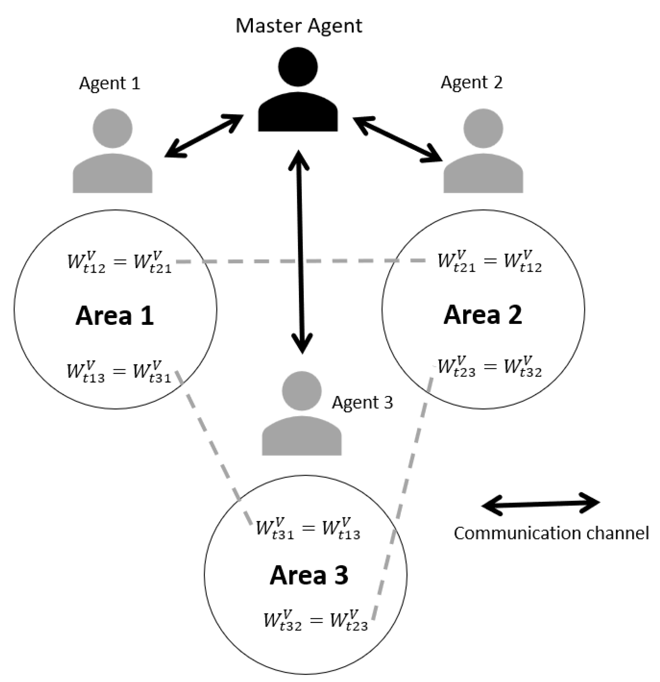
For each of the areas, 24 Ward equivalents related to the 24 periods included in the multi-period analysis were calculated [23]. Communication between areas is performed through a multi-agent approach, which allows communication between each optimizer in each of the areas [42]. Multi-agent master–slave communication was implemented in this work as a system that allows coordination and communication between the different optimization processes involved. In this system, a master agent plays the role of the central coordinator, while slave agents are responsible for performing optimization tasks in specific areas of the system. Equation (23) measures the equality of voltage between each of the nodes where the Ward equivalent is calculated for each area. In this case, $W_{ta}^V$ and $W_{t(a-1)}^V$ are the Ward equivalents in two different areas at time t. If these nodes have equal voltage, there is equivalence between the complete system and each of the areas. This measurement is performed after carrying out the optimization of each of the areas [42].

$$\begin{array}{c}\hfill (W_{ta}^V-W_{t(a-1)}^V)<ϵ,t\in [1,24],a\in [1,A]\end{array}$$

(23)

The master agent is responsible for managing the agents to perform the optimization of each area, showing an example of three areas as shown in Figure 1, following the steps presented below:

1.

The master agent takes the complete system of interest and calculates the Ward equivalent for each of the 24 periods of Area 1, taking into account the initial operating conditions. The calculation of the equivalent is performed on the buses that allow the separation of Area 1 from the other areas. With this result, agent 1 optimizes Area 1.

2.

Taking into account the results obtained in Area 1, the master agent creates for Area 2 the Ward equivalents for the 24 periods, which allow separating Area 2 from the other areas, and demands Agent 2 adjust and optimize area 2.

3.

Taking into account the results of Areas 1 and 2, the master agent calculates the Ward equivalents of the 24 periods for Area 3 and requests Agent 3 adjust and optimize Area 3.

4.

Equation (23) is validated; if the equation is fulfilled, the master agent finishes the optimizer; otherwise, the same procedure, beginning from Item 1, is performed again.

3. Test and Results

The validation of the proposed optimization model was performed using the IEEE 39 and 57-bus test systems, which are widely known in the technical literature. The separation of areas by means of VCA and the selection of pilot nodes for the two test systems selected in this work were carried out taking into account the results obtained in [23,48]. The modeling was implemented in the Python programming language, through the use of the PandaPower [49] and Pyomo [50] libraries. The PandaPower library was used to obtain all the conditions of the power system. The Pyomo library was used to create the presented optimization model, as well as its connection with the BONMIN solver, which provides the solution of the model. It is worth mentioning that, due to the nature of the problem, there was not a guarantee of obtaining globally optimal solutions. In this optimizer, the variables ${\beta }_1$, ${\beta }_2$, and ${\beta }_3$ were used as $3\times {10}^2$, $1\times {10}^{-2}$, and 10, respectively, for the IEEE-39 bus system, and ${\beta }_1$, ${\beta }_2$, and ${\beta }_3$ were used as $3\times {10}^4$, $1\times {10}^{-1}$, and 10, respectively, for the IEEE-57 bus system. This was performed to ensure equal values for each equation and to give equal importance to each part of the equation being optimized.

The MA-MP-ORPD performs the separation of the areas by means of the Ward equivalent, and for each of the areas obtained, a multi-period analysis was performed, which implies time dependence and the use of a demand curve. Figure 2 shows the behavior of the demand curve (in percentage) used to create the 24 periods. In this document, the load conditions are presented through a spring workday load curve available at [51].

3.1. IEEE 39-Bus Test System

This system is composed of 39 nodes, 35 lines, and 11 transformers. Furthermore, 10 generators and 21 loads are incorporated, which are connected to the buses to simulate power generation and demand in the network, as shown in Figure 3. Additionally, the separation by VCA and the selection of the pilot nodes are shown. In Period 11, the system reaches its maximum power with a value of 6254 MW and 1387 MVAr. The initial conditions are obtained from the solution of a base load flow with the PandaPower library, where the values of the transformer taps are in the neutral position.

This system is divided into three voltage control areas [48]. Each area has two pilot nodes in charge of representing and guaranteeing the corresponding voltage profiles, which are marked with an asterisk in Figure 3. The generators in each area feature an adjustable set-point between 0.9 and 1.1 p.u., which is used to regulate the system voltage. Additionally, the transformers have a tap value between 0.9 and 1.1 p.u., with steps of 0.01 p.u. for each tap operation.

3.2. IEEE 57-Bus Test System

This system consists of 57 nodes, 65 lines, and 16 transformers. It also incorporates seven generators and 42 loads, which are connected to the buses to simulate the generation and demand of energy in the network, as shown in Figure 4. Additionally, the separation by VCA and the selection of the pilot buses are shown. In Period 11, the system reaches its maximum power with a value of 1250 MW and 336 MVAr. The initial conditions are obtained from the solution of a base load flow with the PandaPower library, where the values of the transformer taps are in the neutral position.

This system is separated into three areas; each area has two pilot nodes (marked with an asterisk in Figure 4). The generators in each area feature an adjustable set-point between 0.9 and 1.1 p.u., which is used to regulate the system voltage. Additionally, the transformers have a tap value between 0.9 and 1.1 p.u., with steps of 0.01 p.u. for each tap operation. The system has three shunt devices, which are capacitive compensations of 10, 5.9, and 6.3 MVAr located at buses 18, 25, and 53, respectively; four steps were considered for each capacitor.

The values of the control variables for the MA-MP-ORPD in the test systems are presented in Appendix A, which indicates the settings for the capacitors, transformers, and generation voltages for each period of time. In this Appendix, it is possible to verify that all variables remained within their safe operating ranges. All the results presented below correspond to the objective function given by Equation (1). In each case, the result of the multi-area and multi-period optimization (MA-MP-ORPD) was compared with the base case. For reactive power reserves, the multi-period optimization presented in [23] was used for comparative purposes. The base case represents the system condition in which only the active power distribution has been optimized; therefore, there are no objectives related to the voltage set-point nor to reactive power management in the compensation elements and generators. This case starts from the system present in the PandaPower library, by means of which an initial load flow is calculated. The base case is taken as a reference to show the difference between the MP-ORPD optimization result, the MA-MP-ORPD optimization result, and the system input information, which allows understanding how the control variables change.

3.3. Results with the IEEE 39-Bus Test System

The voltage profiles of the pilot nodes in each of the areas are presented in Figure 5. For each pilot node, a reference curve to be followed in voltage control was defined, and it was observed that the optimizer managed to maintain the voltage profile in line with the curves proposed for these nodes. The shape of the proposed voltage profiles allows the development of an operational strategy that defines a safe profile for each of the demand conditions and guarantees the voltage stability of the system.

The changes in transformer taps in each area are shown in Figure 6. Each area has transformers and voltage control elements that the optimizer uses to increase reactive power resources. The condition of performing only one tap movement per period was considered, in order to avoid excessive movements that are not desirable in the operation of these devices and reduce their useful lives. The results showed that the movement of taps was a variable that contributed to a better result, and its use benefited the voltage profiles of the system.

The IEEE 39-bus test system has a high reactive power demand, which is evident in Figure 7, where the red bars represent the base case of the system obtained by load flow using the PandaPower library. The demand profile used, presented in Figure 2, shows that the maximum demand was found in the periods close to Hours 11 and 20, which implies that the reactive power reserves for these periods are lower. The blue bars represent the results obtained with the MP-ORPD optimizer (which is run on the entire system, and then, the results are separated for each area), where it can be seen that good results were obtained compared to the base case, since for all areas, an increase in reactive power reserves was achieved.The green bars show the results of the MA-MP-ORPD on the three VCAs obtained from the system. The multi-area model shows a better performance in increasing reactive power reserves as shown in

Table 2. Increase of reactive power reserves with respect to the base case for each VCA in the IEEE 39-bus test system.

Area	Base Case (MVAr)	MP-ORPD (%)	MA-MP-ORPD (%)
1	18,251	10	26
2	7493	32	52
3	9585	41	59

, where it can be seen that Area 3 had the highest increase with a value of 59%. This was due to the fact that, by having an optimizer that seeks to maximize the reactive power reserves of the system in each area, a greater sensitivity to the particular needs of each VCA is achieved, which correspond to the specific needs present in the normal operation of the interconnected electrical system.

Figure 8 presents the evaluation of the stability index presented in Equation (22) for each node other than the pilot nodes. The boxplot is used to observe the behavior of the $Kv$ index of each bus in every VCA in the 24 periods, using as lower and upper limits of 0.85 p.u. and 1.15 p.u., respectively; this is considered as the safe operating range for evaluating the index presented. Figure 8 shows that the $Kv$ index increased for most of the buses, indicating that the system was far from critical voltages. The $Kv$ index allows knowing the behavior of the voltages in the different buses and to take corrective actions to improve the voltage stability in the most-impacted area.

3.4. Results with the IEEE 57-Bus Test System

This test system presented similar results to the previous network when applying the proposed MA-MP-ORPD. In this case, a voltage profile to be followed was also defined for each of the pilot nodes in order to preserve the voltage stability of the system. The results presented in Figure 9 show that the voltage profiles in the pilot nodes were maintained with respect to the base profiles. It was observed that Area 1 had the lowest voltage profiles due to the higher concentration of demand away from the generation nodes. The base voltage profiles sought to maintain the system voltage profiles at safe values to increase system stability.

Figure 10 shows the most-significant transformer tap changes in each of the system areas. For the most part, the transformers remained in a single tap position, as can be seen in Transformers 15–45 in Area 1. In the transformers presented, a change of one tap position per period was performed and a smaller movement in tap changes was observed in all of them. In addition, it was observed that the taps were maintained to a greater extent at a value lower than 1 p.u. In the capacitive compensators, it was observed that, for all devices and all periods, these were maintained in a single position corresponding to the largest step. This was due to the fact that the number of maneuvers in these elements was penalized, and since the system requires reactive power, these devices operated with the highest reactive capacity they could deliver.

The results of the evaluation of reactive power reserves with respect to the base case are shown in Figure 11, where the results of the MP-ORPD and MA-MP-ORPD are compared. Note that similar results to those presented in the previous system were obtained. The reactive power reserves increased for all periods compared to the base case. In particular, the MA-MP-ORPD obtained better results in the three evaluated areas, although in some periods, the MP-ORPD model performed better; however, considering the power reserve for the whole day, more reserves were obtained with the MA-MP-ORPD model.

Table 3. Increase in reactive power reserves with respect to the base case for each area in the IEEE 57-bus test system.

Area	Base Case (MVAr)	MP-ORPD (%)	MA-MP-ORPD (%)
1	2440	6	20
2	3699	17	24
3	1510	41	57

shows the percentages of increase in reactive power reserves for each of the areas, where it is evident that the multi-area optimization presented the best results with up to a 60% increase in Area 3. This improved performance was due to the model’s ability to increase reactive power reserves by area, focusing on the particular needs of each part of the system to improve the overall system. In this case, the MA-MP-ORPD model offered greater benefits and greater control of reactive power generation in each VCA.

Figure 12 illustrates the evaluation of the $Kv$ stability index presented in Equation (22) for each node other than the pilot nodes. The boxplot shows that, for the IEEE 57-bus test system, there was an increase in the $Kv$ index of most of the buses, which implies that the system presents voltages farther away from their critical values (defined by the same limits used in the IEEE 39-bus test system) after performing the optimization. In Area 1, for Nodes 2, 3, 14, and 15, there was a decrease of the $Kv$ index, which implies that, for these buses, the voltages were closer to their defined critical limits.

3.5. Sensitivity Analysis

A sensitivity analysis was carried out to verify the adaptability of the proposed model to changes in the system conditions.

Table 4. Increase of reactive power reserves with respect to the base case by starting the optimizer at each VCA in the IEEE 39-bus test system.

Area	Base Case (MVAr)	Area 1 (%)	Area 2 (%)	Area 3 (%)
1	18,251	20	18	21
2	7493	24	26	25
3	9585	57	55	59

and

Table 5. Increase of reactive power reserves with respect to the base case by starting the optimizer at each VCA in the IEEE 57-bus test system.

Area	Base Case (MVAr)	Area 1 (%)	Area 2 (%)	Area 3 (%)
1	2440	26	24	24
2	3699	52	54	51
3	1510	59	62	57

show the results of increasing the reactive power reserves when starting the optimization process from different areas, selecting a specific area for its solution. The results obtained indicated that the model did not perform better when starting in a particular area with respect to the results for that area.

4. Conclusions

This paper presented a modeling approach to the optimal reactive power dispatch considering a multi-area system and different time intervals (MA-MP-ORPD). Three main components were considered in the formulation. The first component sought to maintain system voltage profiles within safe operating limits by using pilot nodes defined for each area under analysis. The second component aimed to minimize the number of maneuvers performed by static reactive power compensation devices, avoiding excessive wear and tear and, therefore, increasing the life expectancy of these elements. The third component sought to increase the reactive power reserves of the synchronous generators in each area.

The main feature of the proposed MA-MP-ORPD model lies in its ability to address complex electrical systems separated by voltage control areas and to consider the variation of the system demand in a given time horizon (24 h) in each of these areas. This allows solving the optimization model in reduced systems, i.e., by VCA, but interconnected. The above generated results that met the needs of the complete system, as evidenced by the results of the various tests performed on the test models.

The results of the tests showed that the number of operations on static compensation elements was minimized and that the constraints that limit changes in transformer taps from one period to another were maintained. This results in economic benefits to the owners of the equipment by avoiding excessive wear and preserving its useful life.

Additionally, the use of pilot nodes guarantees an adequate voltage profile in all areas and also reduces the convergence time. The Kv stability index, which measures the proximity of nodes to a critical voltage value, was used to analyze the impact on the system operation. The results showed that, for nodes other than pilot nodes, there was no significant impact that may affect the stable operation of the system. In addition, it was validated that this index, after optimization, did not present significant changes that may cause an operation in non-stable scenarios. The computing times were 5.6 and 14.9 s for the 39- and 57-bus test systems, respectively. The tests were performed on a personal computer with an AMD Ryzen 5 processor running at 3 GHz and 8 GB of RAM. This allowed concluding that the model was adequate to be integrated into the analysis performed by the network operators in medium- and short-term planning.

Future work may explore the possibility of parallelization to reduce the calculation time by dividing the problem into smaller tasks that run simultaneously on multiple processors. This can significantly accelerate the calculation time and improve the problem-solving efficiency. Furthermore, a comparative analysis of some control area partitioning methods that consider demand uncertainty and topological changes of the VCAs may be explored.

References

- Echeverria, D.; Flores, V.; Villa, W.; Cepeda, J. Identificación de Áreas de Control de Voltaje en el Sistema Nacional Interconectado de Ecuador utilizando Minería de Datos. Rev. Técnica Energía 2017, 13, 70–78. [Google Scholar] [CrossRef]
- Rabiee, A.; Parniani, M. Voltage security constrained multi-period optimal reactive power flow using benders and optimality condition decompositions. IEEE Trans. Power Syst. 2013, 28, 696–708. [Google Scholar] [CrossRef]
- Agudelo, L.; López-Lezama, J.M.; Muñoz-Galeano, N. Vulnerability assessment of power systems to intentional attacks using a specialized genetic algorithm. Dyna 2015, 82, 78–84. [Google Scholar] [CrossRef]
- Shaheen, A.M.; El-Sehiemy, R.A.; Hasanien, H.M.; Ginidi, A.R. An improved heap optimization algorithm for efficient energy management based optimal power flow model. Energy 2022, 250, 123795. [Google Scholar] [CrossRef]
- Wu, Q.H.; Ma, J.T. Power system optimal reactive power dispatch using evolutionary programming. IEEE Trans. Power Syst. 1995, 10, 1243–1249. [Google Scholar] [CrossRef] [PubMed]
- Villa-Acevedo, W.M.; López-Lezama, J.M.; Valencia-Velásquez, J.A. A Novel Constraint Handling Approach for the Optimal Reactive Power Dispatch Problem. Energies 2018, 11, 2352. [Google Scholar] [CrossRef]
- Khan, N.H.; Wang, Y.; Tian, D.; Raja, M.A.Z.; Jamal, R.; Muhammad, Y. Design of Fractional Particle Swarm Optimization Gravitational Search Algorithm for Optimal Reactive Power Dispatch Problems. IEEE Access 2020, 8, 146785–146806. [Google Scholar] [CrossRef]
- Laouafi, F.; Boukadoum, A.; Leulmi, S. A Hybrid Formulation between Differential Evolution and Simulated Annealing Algorithms for Optimal Reactive Power Dispatch. Telkomnika Telecommun. Comput. Electron. Control. 2018, 16, 513–524. [Google Scholar] [CrossRef]
- Sidea, D.O.; Picioroaga, I.I.; Tudose, A.M.; Bulac, C.; Tristiu, I. Multi-Objective Particle Swarm optimization Applied on the Optimal Reactive Power Dispatch in Electrical Distribution Systems. In Proceedings of the 2020 International Conference and Exposition on Electrical and Power Engineering (EPE), Iaşi, Romania, 22–23 October 2020; pp. 413–418. [Google Scholar] [CrossRef]
- Martinez-Rojas, M.; Sumper, A.; Gomis-Bellmunt, O.; Sudrià-Andreu, A. Reactive power dispatch in wind farms using particle swarm optimization technique and feasible solutions search. Appl. Energy 2011, 88, 4678–4686. [Google Scholar] [CrossRef]
- Abbasy, A.; Hosseini, S.H. Ant Colony Optimization-Based Approach to Optimal Reactive Power Dispatch: A Comparison of Various Ant Systems. In Proceedings of the 2007 IEEE Power Engineering Society Conference and Exposition in Africa—PowerAfrica, Johannesburg, South Africa, 16–20 July 2007; pp. 1–8. [Google Scholar] [CrossRef]
- Abou El-Ela, A.; Kinawy, A.; El-Sehiemy, R.; Mouwafi, M. Optimal reactive power dispatch using ant colony optimization algorithm. Electr. Eng. 2011, 93, 103–116. [Google Scholar] [CrossRef]
- Rayudu, K.; Yesuratnam, G.; Jayalaxmi, A. Ant colony optimization algorithm based optimal reactive power dispatch to improve voltage stability. In Proceedings of the 2017 International Conference on Circuit, Power and Computing Technologies (ICCPCT), Kollam, India, 20–21 April 2017; pp. 1–6. [Google Scholar] [CrossRef]
- Ayan, K.; Kılıc, U. Artificial bee colony algorithm solution for optimal reactive power flow. Appl. Soft Comput. 2012, 12, 1477–1482. [Google Scholar] [CrossRef]
- Chen, L.; Deng, Z.; Xu, X. Two-Stage Dynamic Reactive Power Dispatch Strategy in Distribution Network Considering the Reactive Power Regulation of Distributed Generations. IEEE Trans. Power Syst. 2019, 34, 1021–1032. [Google Scholar] [CrossRef]
- Gutierrez Rojas, D.; Lopez Lezama, J.; Villa, W. Metaheuristic Techniques Applied to the Optimal Reactive Power Dispatch: A Review. IEEE Lat. Am. Trans. 2016, 14, 2253–2263. [Google Scholar] [CrossRef]
- Mugemanyi, S.; Qu, Z.; Rugema, F.X.; Dong, Y.; Bananeza, C.; Wang, L. Optimal Reactive Power Dispatch Using Chaotic Bat Algorithm. IEEE Access 2020, 8, 65830–65867. [Google Scholar] [CrossRef]
- Ali, A.; Abbas, G.; Keerio, M.U.; Touti, E.; Ahmed, Z.; Alsalman, O.; Kim, Y.S. A Bi-Level Techno-Economic Optimal Reactive Power Dispatch Considering Wind and Solar Power Integration. IEEE Access 2023, 11, 62799–62819. [Google Scholar] [CrossRef]
- Jamal, R.; Men, B.; Khan, N.H. A Novel Nature Inspired Meta-Heuristic Optimization Approach of GWO Optimizer for Optimal Reactive Power Dispatch Problems. IEEE Access 2020, 8, 202596–202610. [Google Scholar] [CrossRef]
- Jamal, R.; Men, B.; Khan, N.H.; Raja, M.A.Z.; Muhammad, Y. Application of Shannon Entropy Implementation Into a Novel Fractional Particle Swarm Optimization Gravitational Search Algorithm (FPSOGSA) for Optimal Reactive Power Dispatch Problem. IEEE Access 2021, 9, 2715–2733. [Google Scholar] [CrossRef]
- Sabir, M.; Ahmad, A.; Ahmed, A.; Siddique, S.; Hashmi, U.A. A Modified Inertia Weight Control of Particle Swarm Optimization for Optimal Reactive Power Dispatch Problem. In Proceedings of the 2021 International Conference on Emerging Power Technologies (ICEPT), Topi, Pakistan, 10–11 April 2021; pp. 1–6. [Google Scholar] [CrossRef]
- Viegas da Silva, M.; Home Ortiz, J.M.; Pourakbari-Kasmaei, M.; Sanches Mantovani, J.R. Convex Formulation for Optimal Active and Reactive Power Dispatch. IEEE Lat. Am. Trans. 2022, 20, 787–798. [Google Scholar] [CrossRef]
- Morán-Burgos, J.A.; Sierra-Aguilar, J.E.; Villa-Acevedo, W.M.; López-Lezama, J.M. A Multi-Period Optimal Reactive Power Dispatch Approach Considering Multiple Operative Goals. Appl. Sci. 2021, 11, 8535. [Google Scholar] [CrossRef]
- Tamayo, D.C.L.; Villa-Acevedo, W.M.; López-Lezama, J.M. Despacho óptimo de potencia reactiva considerando un abordaje multiperiodo. Inf. Tecnológica 2021, 32, 179–190. [Google Scholar] [CrossRef]
- Gómez Bedoya, D.A. Metodología Para el Análisis de Estabilidad de Tensión Mediante la División de Redes en Áreas de Control. 2014. Available online: https://repositorio.unal.edu.co/handle/unal/21804 (accessed on 14 February 2023).
- Salama, H.S.; Vokony, I. Voltage stability indices–A comparison and a review. Comput. Electr. Eng. 2022, 98, 107743. [Google Scholar] [CrossRef]
- Althowibi, F.A.; Mustafa, M.W. On-line voltage collapse indicator for power systems. In Proceedings of the 2010 IEEE International Conference on Power and Energy, Kuala Lumpur, Malaysia, 29 November–1 December 2010; pp. 408–413. [Google Scholar] [CrossRef]
- Leonardi, B.; Ajjarapu, V. An approach for real time voltage stability margin control via reactive power reserve sensitivities. IEEE Trans. Power Syst. 2013, 28, 615–625. [Google Scholar] [CrossRef]
- Terzija, V.; Valverde, G.; Cai, D.; Regulski, P.; Madani, V.; Fitch, J.; Skok, S.; Begovic, M.M.; Phadke, A. Wide-Area Monitoring, Protection, and Control of Future Electric Power Networks. Proc. IEEE 2011, 99, 80–93. [Google Scholar] [CrossRef]
- Kessel, P.; Glavitsch, H. Estimating the Voltage Stability of a Power System. IEEE Trans. Power Deliv. 1986, 1, 346–354. [Google Scholar] [CrossRef]
- Sanz, F.A.; Ramirez, J.M.; Correa, R.E. Statistical estimation of power system vulnerability. In Proceedings of the 2013 North American Power Symposium (NAPS), Manhattan, KS, USA, 22–24 September 2013; pp. 1–6. [Google Scholar] [CrossRef]
- Kataoka, Y.; Watanabe, M.; Iwamoto, S. A New Voltage Stability Index Considering Voltage Limits. In Proceedings of the 2006 IEEE PES Power Systems Conference and Exposition, Atlanta, GA, USA, 29 October–1 November 2006; pp. 1878–1883. [Google Scholar] [CrossRef]
- Schlueter, R. A voltage stability security assessment method. IEEE Trans. Power Syst. 1998, 13, 1423–1438. [Google Scholar] [CrossRef] [PubMed]
- Villa, W.M.; Rueda, J.L.; Torres, S.; Peralta, W.H. Identification of voltage control areas in power systems with large scale wind power integration. In Proceedings of the 2012 Sixth IEEE/PES Transmission and Distribution: Latin America Conference and Exposition (T&D-LA), Montevideo, Uruguay, 3–5 September 2012; pp. 1–7. [Google Scholar] [CrossRef]
- Daher, N.A.; Mougharbel, I.; Saad, M.; Kanaan, H.Y.; Asber, D. Pilot buses selection based on reduced Jacobian matrix. In Proceedings of the 2015 IEEE International Conference on Smart Energy Grid Engineering (SEGE), Oshawa, ON, Canada, 17–19 August 2015; pp. 1–7. [Google Scholar] [CrossRef]
- Grigoras, G.; Neagu, B.C.; Scarlatache, F.; Ciobanu, R.C. Identification of pilot nodes for secondary voltage control using K-means clustering algorithm. In Proceedings of the 2017 IEEE 26th International Symposium on Industrial Electronics (ISIE), Edinburgh, UK, 19–21 June 2017; pp. 106–110. [Google Scholar] [CrossRef]
- Lashkar Ara, A.; Kazemi, A.; Gahramani, S.; Behshad, M. Optimal reactive power flow using multi-objective mathematical programming. Sci. Iran. 2012, 19, 1829–1836. [Google Scholar] [CrossRef]
- Satsangi, S.; Saini, A.; Saraswat, A. Voltage control areas for reactive power management using clustering approach in deregulated power system. In Proceedings of the International Conference on Sustainable Energy and Intelligent Systems (SEISCON 2011), Chennai, India, 20–22 July 2011; pp. 409–415. [Google Scholar] [CrossRef]
- Deeb, N.; Shahidehpour, S. Cross decomposition for multi-area optimal reactive power planning. IEEE Trans. Power Syst. 1993, 8, 1539–1544. [Google Scholar] [CrossRef]
- Liu, Z.W.; Liu, M.B. Distributed Reactive Power Optimization Computing in Multi-area Power Systems Using Ward Equivalent. In Proceedings of the 2010 International Conference on Electrical and Control Engineering, Wuhan, China, 25–27 June 2010; pp. 3659–3663. [Google Scholar] [CrossRef]
- Liu, Z.W.; Liu, M.B.; Xia, W.B. Comparison of Multi-area Reactive Power Optimization Parallel Algorithm Based on Ward and REI Equivalent. Energy Procedia 2012, 14, 1580–1589. [Google Scholar] [CrossRef]
- Pham, H.V.; Ahmed, S.N.; Erlich, I. Multi-agent system based solution of the optimal reactive power dispatch problem in autonomously operated multi-area systems. In Proceedings of the 2015 IEEE Eindhoven PowerTech, Eindhoven, The Netherlands, 29 June–2 July 2015; pp. 1–6. [Google Scholar] [CrossRef]
- Ibrahim, T.; Rubira, T.T.D.; Rosso, A.D.; Patel, M.; Guggilam, S.; Mohamed, A.A. Alternating Optimization Approach for Voltage-Secure Multi-Period Optimal Reactive Power Dispatch. IEEE Trans. Power Syst. 2022, 37, 3805–3816. [Google Scholar] [CrossRef]
- Muhammad, Y.; Khan, R.; Raja, M.A.Z.; Ullah, F.; Chaudhary, N.I.; He, Y. Solution of optimal reactive power dispatch with FACTS devices: A survey. Energy Rep. 2020, 6, 2211–2229. [Google Scholar] [CrossRef]
- Van Amerongen, R.; van Meeteren, H.P. A Generalised Ward Equivalent for Security Analysis. IEEE Trans. Power Appar. Syst. 1982, PAS-101, 1519–1526. [Google Scholar] [CrossRef]
- Lo, K.; Peng, L.; Macqueen, J.; Ekwue, A.; Cheng, D. An extended ward equivalent approach for power system security assessment. Electr. Power Syst. Res. 1997, 42, 181–188. [Google Scholar] [CrossRef]
- Baldwin, T.; Mili, L.; Phadke, A. Dynamic Ward equivalents for transient stability analysis. IEEE Trans. Power Syst. 1994, 9, 59–67. [Google Scholar] [CrossRef]
- Villa-Acevedo, W.M.; López-Lezama, J.M.; Colomé, D.G.; Cepeda, J. Long-term voltage stability monitoring of power system areas using a kernel extreme learning machine approach. Alex. Eng. J. 2022, 61, 1353–1367. [Google Scholar] [CrossRef]
- Thurner, L.; Scheidler, A.; Schäfer, F.; Menke, J.; Dollichon, J.; Meier, F.; Meinecke, S.; Braun, M. Pandapower—An Open-Source Python Tool for Convenient Modeling, Analysis, and Optimization of Electric Power Systems. IEEE Trans. Power Syst. 2018, 33, 6510–6521. [Google Scholar] [CrossRef]
- Bynum, M.L.; Hackebeil, G.A.; Hart, W.E.; Laird, C.D.; Nicholson, B.L.; Siirola, J.D.; Watson, J.P.; Woodruff, D.L. Pyomo–Pptimization Modeling in Python, 3rd ed.; Springer Science & Business Media: Berlin/Heidelberg, Germany, 2021; Volume 67. [Google Scholar]
- Grigg, C.; Wong, P.; Albrecht, P.; Allan, R.; Bhavaraju, M.; Billinton, R.; Chen, Q.; Fong, C.; Haddad, S.; Kuruganty, S.; et al. The IEEE Reliability Test System-1996. A report prepared by the Reliability Test System Task Force of the Application of Probability Methods Subcommittee. IEEE Trans. Power Syst. 1999, 14, 1010–1020. [Google Scholar] [CrossRef]
Figure 1.
Master agent communication for the connection of three electrical areas.
Figure 2.
Load profile (%) for the 24 periods of time.
Figure 3.
IEEE 39-bus test system with VCA and pilot nodes.
Figure 4.
IEEE 57-bus test system with VCA and pilot nodes.
Figure 5.
Voltage profile of the pilot nodes for the three VCAs in the IEEE 39-bus test system.
Figure 6.
Transformer tap positions (values expressed in p.u.) of the three VACs in the IEEE 39-bus test system.
Figure 7.
Generator reactive power reserves per VCA in the IEEE 39-bus test system.
Figure 8.
stability index of the buses other than the pilot nodes for each area in the IEEE 39-bus test system.
Figure 9.
Voltage profile of the pilot nodes for the three VCAs in the IEEE 57-bus test system.
Figure 10.
Transformer tap positions (values expressed in p.u.) of the three areas in the IEEE 57-bus test system.
Figure 11.
Reactive power reserves of all generators for each area in the IEEE 57-bus test system.
Figure 12.
stability index of the buses other than the pilot nodes for each area in the IEEE 57-bus test system.