
Performance Assessment of Horizontal Ground Heat Exchangers under a Greenhouse in Quebec, Canada
by
 , ,
, ,
Xavier Léveillée-Dallaire
1,*, 
Jasmin Raymond
1,*,
Jónas Þór Snæbjörnsson
2,
Hikari Fujii
3 and
Hubert Langevin
4 1
Centre Eau Terre Environnement, Institut National de la Recherche Scientifique, 490 rue de la Couronne, Québec, QC G1K 9A9, Canada
2
Iceland School of Energy, Reykjavik University, 102 Reykjavík, Iceland
3
Graduate School of International Resource Sciences, Akita University, Akita 010-8502, Japan
4
Géotherma Solutions Inc., Québec, QC G1K 9A9, Canada
*
Authors to whom correspondence should be addressed.
Energies 2023, 16(15), 5596; https://doi.org/10.3390/en16155596
Submission received: 27 June 2023
/
Revised: 17 July 2023
/
Accepted: 21 July 2023
/
Published: 25 July 2023
(This article belongs to the Section J: Thermal Management)
Abstract
:Among the various approaches to agriculture, urban greenhouse farming has gained attention for its ability to address food security and disruptions to global food supply chains. However, the increasing impact of climate change and global warming necessitates sustainable methods for heating and cooling these greenhouses. In this study, we focused on the potential of slinky-coil horizontal ground heat exchangers (HGHEs) to meet the energy demands of urban greenhouses, assuming they are installed beneath the greenhouse to optimize space utilization. Climate data, an energy consumption profile for a greenhouse being designed in La Pocatière (Québec, Canada) and in-situ ground thermal properties assessments were used to build numerical models using FEFLOW and to evaluate the performance of the HGHEs simulated. Four scenarios were simulated and compared to a base case, considering the greenhouse’s maintenance of a constant temperature above an HGHE limited to the greenhouse’s dimensions. Our findings reveal that a minimum of 7.1% and 26.5% of the total heating and cooling loads of a small greenhouse (133 m2 area) can be covered by HGHEs installed at a 1.5 m depth when there is no greenhouse above. When installed under a greenhouse with a constant inside temperature of 21 °C, the coverage for heating loads increases to 22.8%, while cooling loads decrease to 24.2%. Sensitivity analysis demonstrates that the constant temperature in the greenhouse reduces the system’s reliance on surface temperature fluctuations for both heating and cooling, albeit with reduced efficiency for cooling.
1. Introduction
Urban agriculture has been developed throughout history, particularly during times of crisis, where residents have come to grow fruits and vegetables in community or personal gardens to access a direct food source [1]. The COVID-19 pandemic is a good example of such a world crisis that triggered food insecurity in cities [2,3]. Urban agriculture has emerged to address these issues and allow the production of fresh and local goods to avoid disruptions to global food supply chains. While this reduces food insecurities and increases social well-being, this agricultural method is associated with high costs and constraints [4]. A citizen’s socioeconomic status and access to land on which personal gardening is possible are two important constraints that make personal gardens only affordable for a small proportion of the population [5]. Therefore, social companies, community-based organizations and municipal initiatives play a key role in improving food security in unprivileged districts [6], considering the development of social economy initiatives can contribute to food security in neighborhoods.
Greenhouses are becoming increasingly popular for agriculture due to their high output, which is 10–20 times greater per unit area than outdoor production [7]. However, maintaining a controlled temperature in these environments induces significant energy costs. To avoid damaging plants, the air temperature must remain within a specific range, with temperature variations smaller than 5–7 °C [8]. As a result, the majority of the energy consumed for greenhouse operations goes toward heating the building, while the rest is used to provide electrical apparatus and food transportation [9]. These factors reveal a significant challenge for greenhouse growers in cold regions who must find affordable solutions.
Climate change and global warming due to anthropogenic nature are major societal concerns where CO2 emissions must be reduced [10]. Hence, the transition toward sustainable renewable energies is important for decarbonising the energy sector. It is therefore critical to provide energy to urban greenhouses according to (1) renewable energy sources, which have a lower carbon footprint compared to traditional fossil fuels; (2) lower energy dependence, where operators will reduce their vulnerability to cost fluctuations and energy supplies disruptions [11]; and (3) social acceptance, where using renewable energies can enhance the public image and reputation of environmentally responsible food producers.
Ground-source heat pump systems (GSHP) account for most of the geothermal applications in direct use, with 71.6% of the installed capacity and 59.2% of annual energy consumption reported in 2020 [7]. However, these systems have higher installation costs compared to traditional heating systems [12]. There are two main types of geothermal heat exchangers: open loops (groundwater or surface water) and closed loops. The open loops installed in aquifers or surface water circulate water from an aquifer, lake, or pond to the heat pump; however, this method is less common, as it requires a nearby water source or specific hydrogeological conditions. Ground-coupled heat pumps commonly use closed-loop heat exchangers installed in boreholes or trenches, given they can be installed everywhere.
Slinky-coil horizontal ground heat exchangers (HGHEs) can be a cost-effective method for reducing GSHP system installation costs, given they only require shallow excavations instead of borehole drilling. However, this type of HGHE requires a decent amount of space to bury the heat exchange pipes, which are exposed to land area problems when a building is located in a limited space. However, optimization techniques can be employed to reduce the land area needed. For example, the geothermal system can be combined with another type of heating system or the heat exchange rate per unit of the land area can be improved by optimizing the system design [13,14,15]. Greenhouses can be compatible with such hybrid geothermal systems relying on HGHEs, given their floors are often made of unconsolidated soils, which facilitate installation.
Chong et al. [16] developed a slinky HGHE numerical model using the ANSYS Fluent software, testing five different setting configurations of 0.25 m, 0.5 m, 1.0 m, 2.0 m and 3.0 m with a diameter of 0.8 m, 1 m and 1.2 m. The results suggested that reducing the coil pitch could improve the system’s overall performance, reduce the system’s thermal resistivity by 20%, and decrease the overall excavation costs by 15%. They also concluded that local ground thermal and hydraulic properties highly influenced the system’s performance.
Tang et al. [17] modeled a numerical slinky-coil HGHE involving an atmosphere–soil–HGHE interaction, validating the model with a local temperature probe and comparing measured temperatures to a simulated temperature. Their work demonstrated that there is no significant difference in the outlet fluid temperature when the depth of the HGHE is increased from 0.5 m to 1 m. The study points out that numerical simulations are important in the case of an atmosphere–soil–HGHE interaction.
Larwa et al. [18] suggest that slinky-type ground heat exchangers can be modeled using a one-dimensional model. They carried out experimental investigations of heat transfer between hot water flowing through a slinky-coil heat exchanger and the surrounding ground. Using an analytical solution based on the ring source model, they analyzed the measurements taken on a slinky-coil HGHE at a depth of 0.5 m for 3 days. They concluded that when the pitch is small, the temperature distribution in the surrounding ground can be approximated using a one-dimensional method. This simplification assumes that the heat transfer in the ground is similar to that of a flat slab. Here, using a one-dimension model simplifies the problem by neglecting any variations in temperature in other directions.
Wu et al. [19] investigated the thermal performance of a slinky-coil HGHE coupled to a GSHP system for different coil diameters and slinky interval distances. They validated experimental measurements with 3D numerical simulations of such systems using ANSYS Fluent software. The results show that the COP decreased with the running time and changed with ambient environmental conditions. Numerical simulations demonstrated that there is no significant difference caused by variations in the coil diameter in the specific heat extraction of the slinky heat exchanger.
Xing et al. [20] studied different approaches to simulating under-building HGHEs installed under building foundations by comparing an analytical and a numerical model with experimental measurements. The analytical model is based on a superposition of line sources and sinks, while the numerical model uses a two-dimensional finite volume based on a superposition developed in the HVACSIM+ environment. To assess the impact of ambient temperature and environment on the performance of such a system, they operated both models at six different sites across the USA. The results show that, while the analytical models are associated with excessive errors, numerical models are time-consuming. They recommended the use of a one-dimensional ground temperature numerical model, which would require little computation time.
Fujii et al. [13,14] numerically modeled a slinky HGHE and the surrounding soil using the finite-element software FEFLOW [21]. A comparison between the numerical model and a thermal response test (TRT) experiment on the HGHE was made to validate the simulation approach. The results obtained from their HGHE thin-plate numerical simulations revealed that when using the thin plate model, pipe and fluid thermal conductivity of 0.025 W m−1 K−1 to 0.045 W m−1 K−1, respectively, tends to reproduce TRT data and the in-situin-situ operation conditions. This present study used the same approach as that developed by Fujii et al. [13,14] since slinky-coil HGHEs are difficult to model. The heat exchange rate per unit length of the straight horizontal heat exchange pipes is significantly lower than that obtained with a vertical ground heat exchanger because shallow ground temperature is affected by seasonal air temperature variations, and dry soils near the ground surface have relatively low thermal conductivity. Using slinky-coil heat exchange pipes instead of straight pipes is, therefore, a good alternative to optimize the HGHEs’ design and reduce trench length, which can facilitate the development of such a system, even in cases of limited land availability [14].
This work provides a comprehensive assessment of the heating and cooling capacity of HGHEs in the context of urban greenhouse systems. By considering different scenarios and incorporating a sensitivity analysis, we offer a deeper understanding of the different interactions between the building and the HGHE. The work achieved also explored the use of HGHEs for greenhouses, for which limited has been made. The practical aspect of this study is also noteworthy, providing insights for practitioners aiming to improve sustainability of heating and cooling. Our work finally showed that a finite-element simulator such as FEFLOW [21] could be used in such practical cases for HGHE under a greenhouse, which is not initially covered by the software.
In urban areas, there is little land space to install HGHEs. Therefore, it seems important to know if HGHEs installed under the limited surface of a building, such as a greenhouse, can cover significant heating and cooling loads. It is assumed that HGHEs covering a limited area located under a greenhouse can be attractive to users because of their reduced installation cost but would likely not cover the full heating or cooling loads of the greenhouse when installed in a continental humid climate like that of Quebec, Canada, where the heating demand is high in winter. Thus, numerical simulations using FEFLOW [21] were made following the work conducted by Fujii et al. [13,14] to evaluate the percentage of greenhouse heating and cooling loads that can be covered with an HGHE of limited surface area installed under a greenhouse. This approach combines Fujii’s model [13,14] with an actual greenhouse energy consumption profile, allowing for the testing and evaluation of the system’s potential through a 5-year simulation. This methodology serves as a valuable practical application tool, providing insights and data for assessing the system’s performance similar to real-world scenarios.
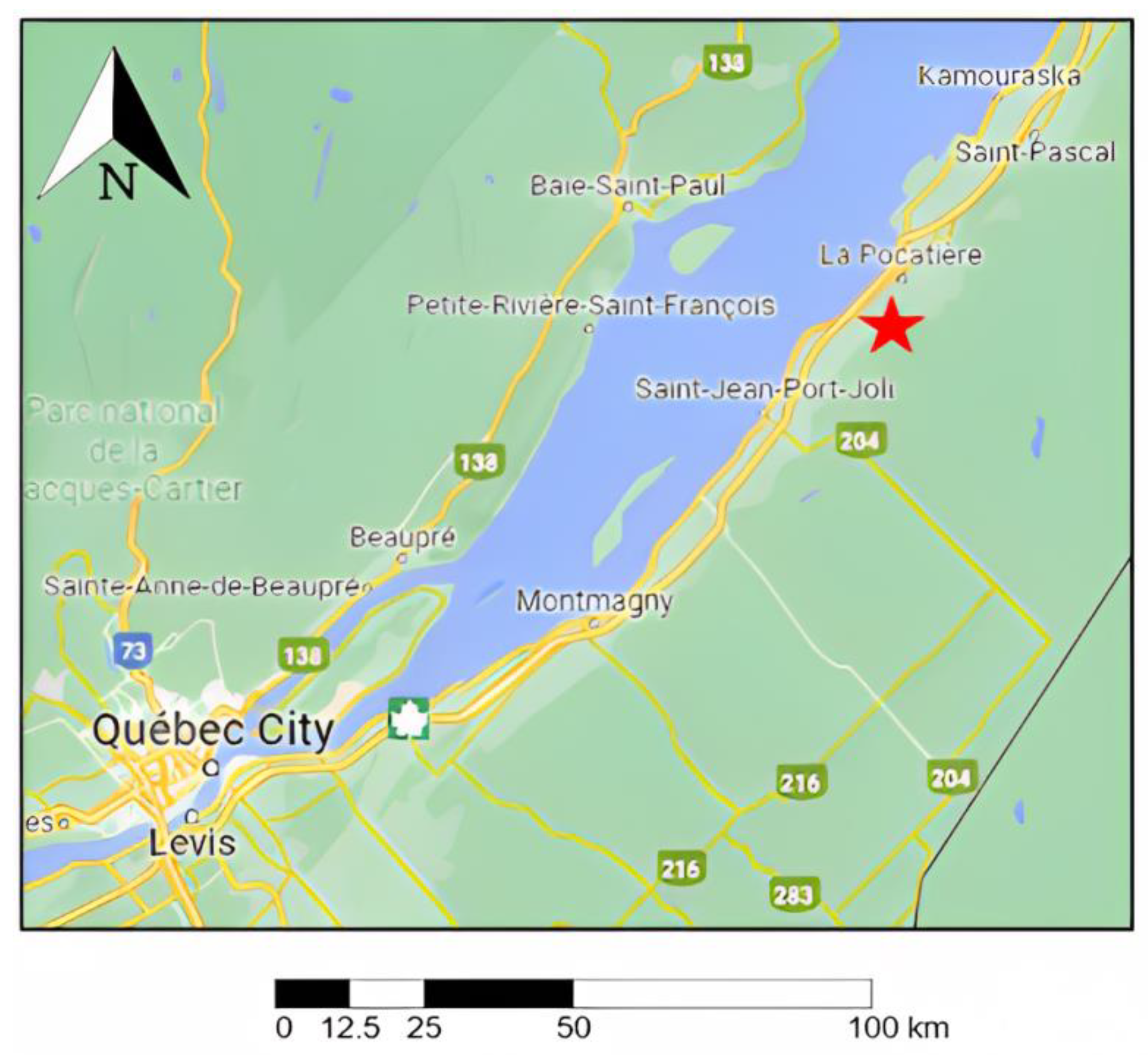
It is important to assess the effect of the greenhouse on such a system, considering local ground thermal properties, ambient and greenhouse air temperature and building energy consumption. A field site was chosen and characterized for this study, aiming to provide information and guidance to integrate HGHEs in greenhouses located in a cold continental humid climate such as Quebec. The Cégep de La Pocatière is planning to build an enclosed greenhouse and complementary research buildings (Figure 1). The project aims to demonstrate that such a research complex can be air-conditioned mainly with renewable energy sources, such as geothermal heat pump systems. A hybrid heating system is envisioned, and the HGHE would be installed below the greenhouse to minimize installation costs, knowing that the system can only fulfill part of the heating and cooling needs. Auxiliary heating and cooling sources would be needed to cover the full heating and cooling loads of the greenhouse. This site was consequently chosen to conduct the study, although obtained conclusions can provide guidelines for other greenhouses in a similar setting.
2. Background Information
2.1. Previous Site Studies
The site is in the province of Quebec, Canada, more precisely in La Pocatière (Figure 1). The projected dimensions of the greenhouse are 14.6 m × 9.1 m, for a total of 133 m2 with a height of 6.1 m. Work was conducted to evaluate the energy consumption of the greenhouse, and an in-situ subsurface characterisation was achieved to evaluate the pre-feasibility of a shallow geothermal system based on the land area available.
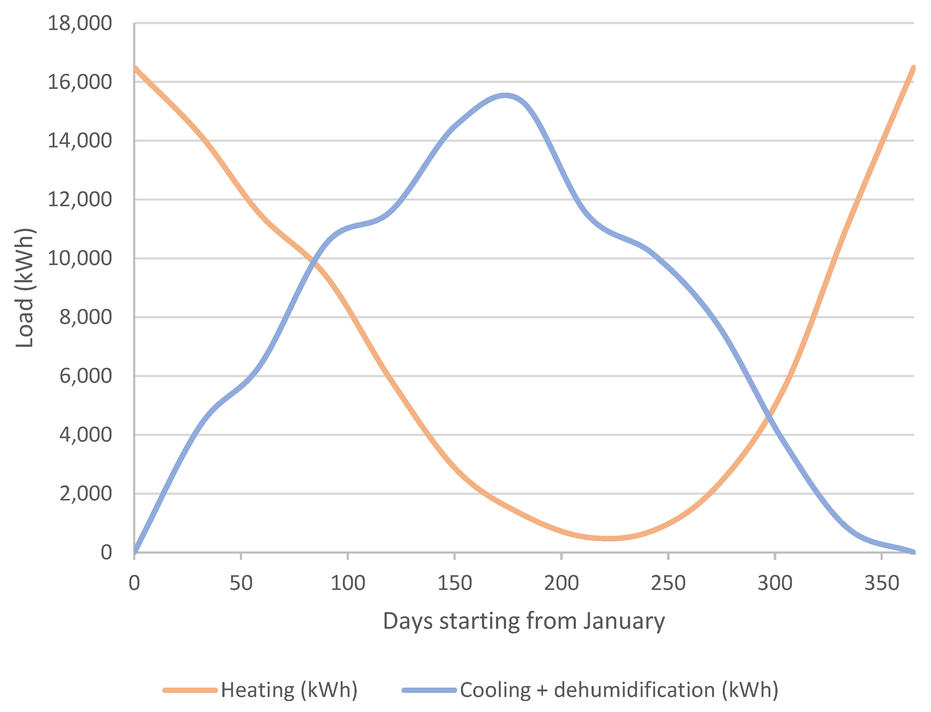
An energy analysis study to simulate a greenhouse in a controlled environment was conducted prior to this study by Enerprox Inc. (Québec, QC, Canada), which was mandated by the Cégep to define the energy consumption profile for three scenarios: an open greenhouse, a semi-open greenhouse and a closed greenhouse [22]. Their study aimed to maintain vapor pressure deficit conditions to optimize plant growth conditions, control the airflow and CO2 injection and optimize energy use. The study resulted in an energy consumption profile for heating and cooling, considering dehumidification for the open and closed greenhouse. The consumption profile provides the average and maximum monthly energy to heat and cool the building. The energy profile displays both heating and cooling demand; therefore, the higher consumption is only considered to determine whether each month belongs to a heating or cooling period. Heating-dominated periods are associated with the months of October to February, while cooling-dominated periods are associated with the months of March to September. The energy profile simulating a closed greenhouse was chosen for this study (Figure 2).
Géotherma Solutions Inc. (Québec, QC, Canada) was also mandated by the Cégep for a pre-feasibility study to assess the required length for two types of shallow geothermal heat exchanger systems according to the energy profile provided by Enerprox Inc. [23]. Their study included field and laboratory work to assess the in-situ thermal conductivity and thermal diffusivity of the ground. Three soil samples were collected to perform laboratory needle probe analyses, and two in-situ oscillatory thermal response tests (OTRT) [24] were also performed. Shallow geothermal heat-exchanger system simulations were then performed using these analyses.
The type of soil encountered at the study site is clayey silt and rock blocks with a diameter that can be greater than 300 mm [23]. The K2DPro Decagon needle probe was used for soil thermal property analysis in saturated and in-situ conditions using the infinite line source equation in the transitional regime. Measurements made on samples do not represent the whole field area since only small samples were needed to use the needle probe method in the laboratory. Therefore, the samples only represented the clayey silt matrix. The SH-1 needle was used to define both the thermal conductivity and heat capacity of the material. Constant heat injection TRT was performed in two different trenches to better evaluate the in-situin-situ ground conditions since it was possible to investigate the effective thermal conductivity of the clayey silt matrix and the rock blocks found at the study site. However, these tests cannot be used to evaluate the ground heat capacity. Thus, OTRT [24] was used to determine the effective ground heat capacity. Two in-situ OTRTs were performed in two different trenches using a 3-meter-long heating cable and five temperature sensors. Ground heat capacity and thermal conductivity were chosen according to the firm’s study (Table 1) [23].
2.2. Ground Temperature
The numerical model temperature at the ground surface was defined using the following Equation (1), aiming to evaluate the ground temperature at a specific time from the historic air temperature [25].
where and (K) are the ground surface and ambient temperatures, respectively. This empirical relationship was developed considering the ambient temperature, the wind velocity and the solar radiation to calculate the ground temperature with a simple approximation in Canada. , from the monthly average temperature of the climate normal, was determined for La Pocatière at an Environment and Climate Change Canada meteorological station between 1981 and 2010 [26] and was used for the ground surface temperature assessment. The months of December, January and February are covered by snow, which acts as an isolation layer for the ground. Based on the numerical simulations, the ground temperature at the surface during this period was therefore considered −1 °C [27], providing the resulting ground surface temperature profile provided in Table 2.
Due to a lack of information and work on the matter, the undisturbed ground temperature is not known for the greenhouse site. The simplification proposed by Ouzzane was also used to calculate the undisturbed ground temperature at a greater depth (~20 m) by considering the average annual ambient air temperature. This revealed an undisturbed ground temperature of 9.1 °C. This value was compared with the data measured in the surrounding area for validation. The average undisturbed ground temperature was evaluated for six locations in Quebec City, 120 km from La Pocatière. The average ground temperature, measured at a depth of more than 20 m in Quebec City, is 9.2 °C [28], and that, calculated with Ouzzane’s empirical equation for the same location, is 9.1 °C. Therefore, an undisturbed ground temperature of 9.1 °C at a depth of 20 m for La Pocatière seems reasonable to use for the numerical simulations of this study.
3. Materials and Methods
3.1. FEFLOW Model for HGHE
3.1.1. Conceptual Model
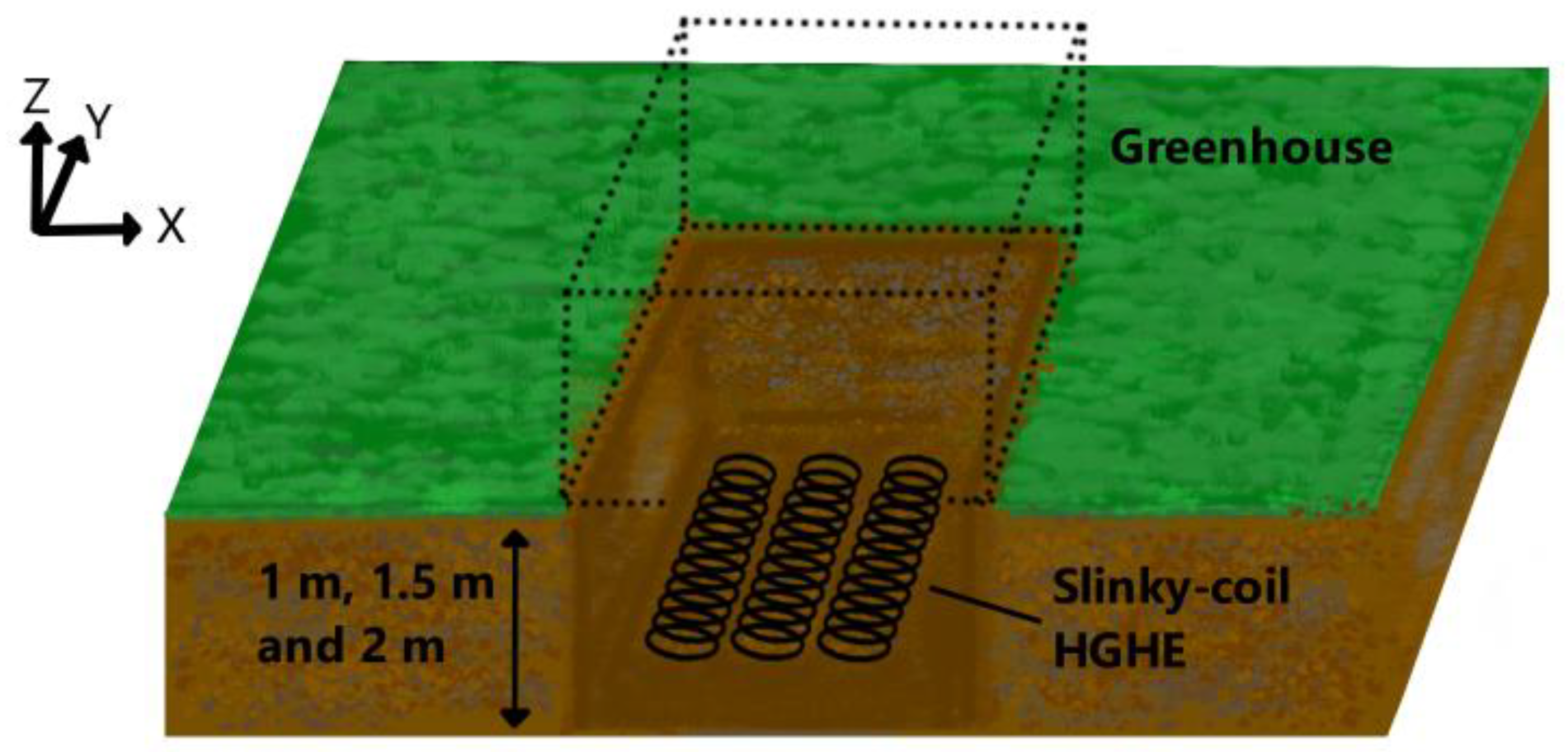
An example of an HGHE is presented in Figure 3, where excavations with slinky-coil pipes were simulated at depths of 1 m, 1.5 m and 2 m.
The simulations of the HGHE operation were conducted using the software FEFLOW [21]. The approach was based on the work by Fujii et al. [13,14]. The following equations model the mass and heat transport in the ground. The first is the mass conversation Equation (2), followed by the momentum conservation Equation (3) and the energy conservation Equation (4):
where is the porosity (-), is the gas density (kg m−3), α is the ground thermal diffusivity (m2 s−1), is the vector of pore velocity (m s1), Qρ is the fluid mass sink/source (s−1), QT is the source of heat (kg m−1 s−3), is the permeability tensor (m2), is the dynamic viscosity of gas (kg m−1 s−1), is the gas pressure (Pa), is Fourier’s heat flux vector (kg s−3), is the gravitational vector (m s−2), are the Cartesian coordinates (m), and is the internal (thermal) energy density (m2 s−2).
3.1.2. Model Geometry
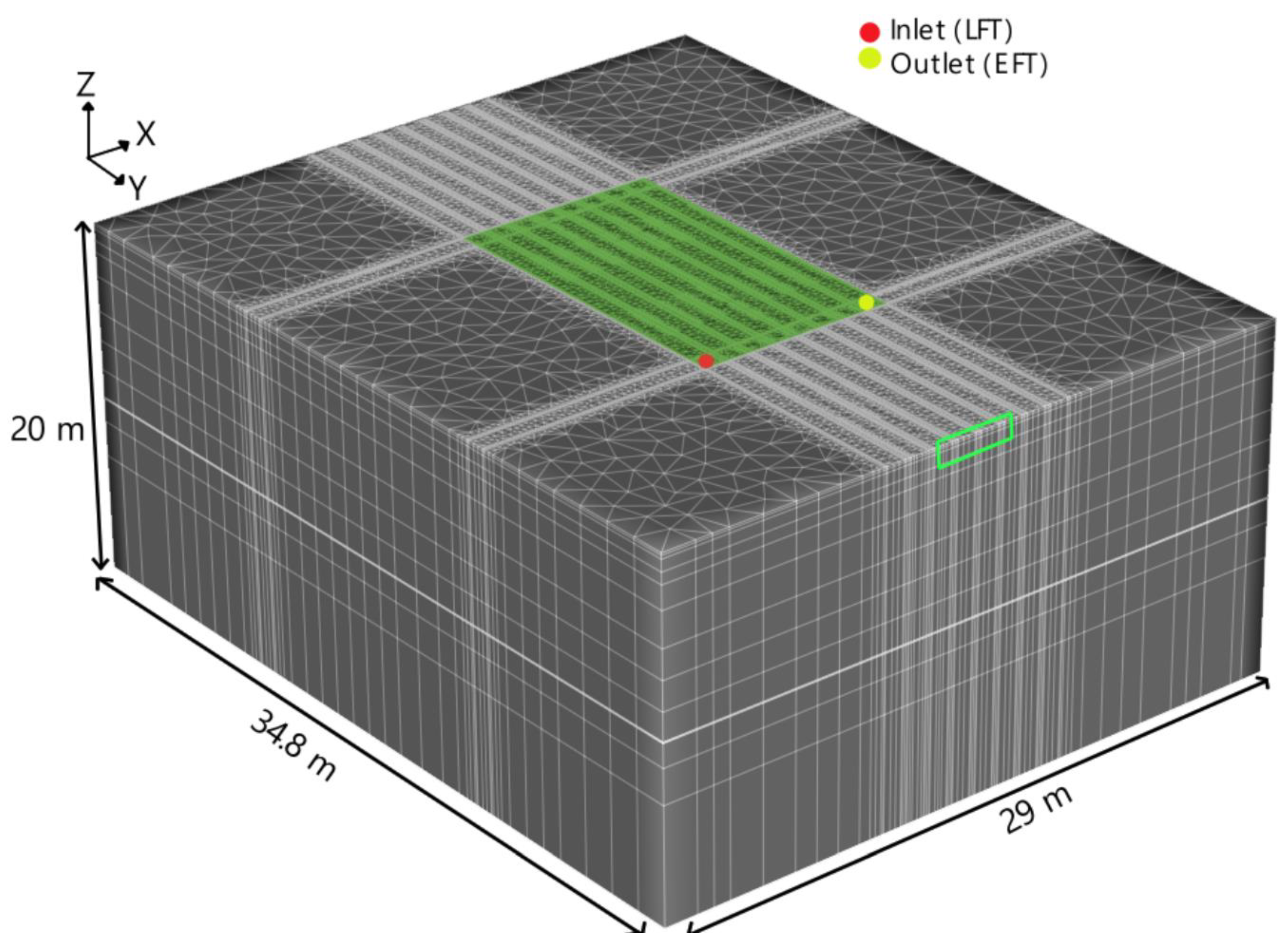
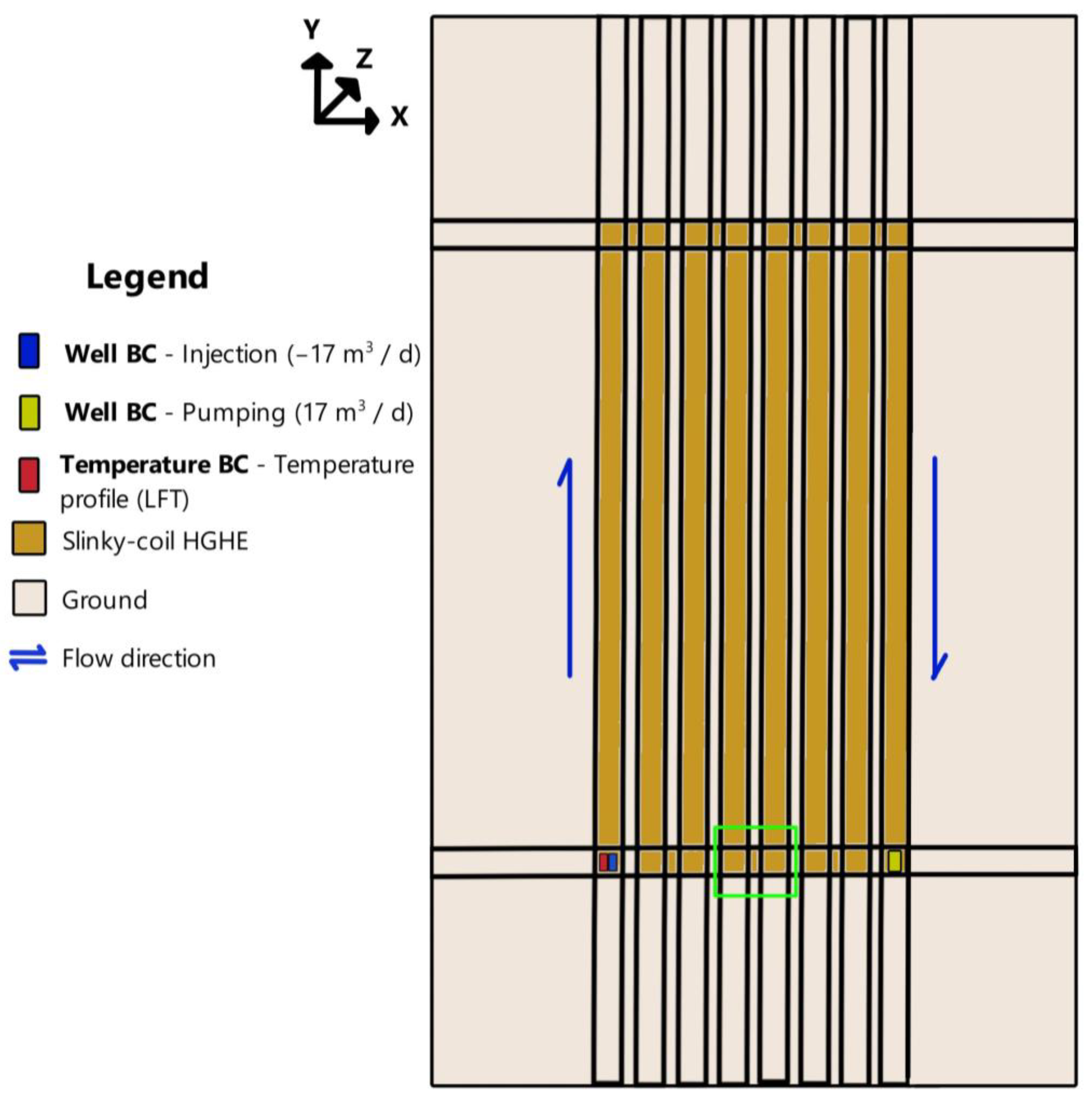
The numerical model is presented in Figure 4, where the green area consists of grids representing the slinky-coil HGHE. The inlet and outlet, where the heat pump leaving fluid temperature (LFT) and entering fluid temperature (EFT) are, respectively, calculated, are shown by the red and yellow dots.
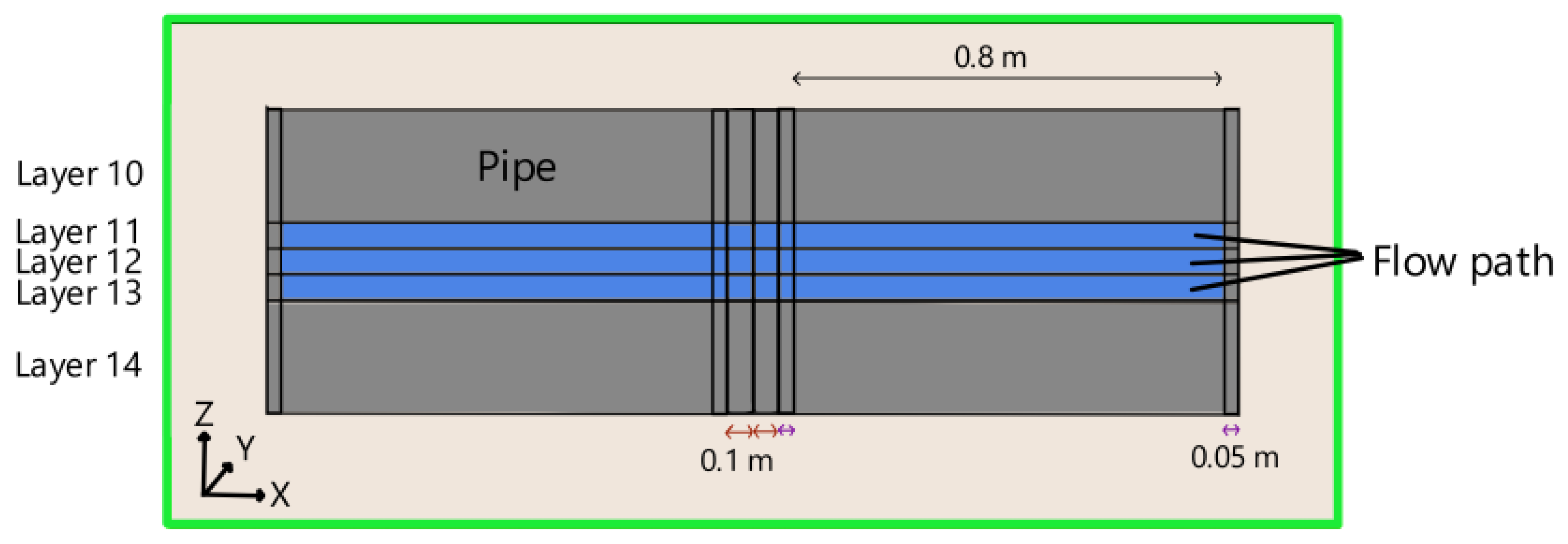
Since slinky-coil HGHE modeling can require heavy computing time, Fujii et al. [13,14] proposed to model a thin flat plate instead of fully discretizing the HGHE, which results in a faster computation time and similar results as obtained with fully discretized models. Although it is possible to reproduce the coil shape in a fully discretized model, it is not practical from a time perspective. The resulting thin plate model is composed of three parts: the flow path, the pipes and the ground. The HGHE is composed of the flow path and the pipes; however, those two components have different thermal and hydraulic properties. The thin plate model is shown in Figure 5 as an excerpt (the small green box) from the 3D model shown in Figure 4. It is assumed to have a length equal to the HGHE trench length and a width equal to the slinky-coil inner diameter. In order to match the arrival time of the heat transfer medium from the heat exchanger inlet to the heat exchanger outlet between the numerical model and the field test results, the volume of the thin plate is equal to the volume of the flow channel in the slinky-coil HGHE (Figure 4 and Figure 5). The thickness of the flow path in the thin plate on the z-axis is calculated using Equation (5) [14]:
where z, dinner, L, X and W are the total thickness of the grid corresponding to the flow path (m), inner diameter of the polyethylene pipe (m), total length of the buried slinky-coil HGHE (m), length of the trench in which the slinky-coil HGHE is buried (m) and the width of the trench where the slinky-coil HGHE is buried (m).
The flow path is therefore composed of three layers, with one layer above and below representing the pipe walls (Figure 5). The gray part represents the pipe walls, while the blue part represents the flow path where the fluid flows. The flow path has a high porosity and high hydraulic conductivity, while the rest of the model has very low porosity and hydraulic conductivity. This makes water flow in the pipes from the inlet to the outlet. Specific values for the HGHE thermal conductivity and heat capacity for both the polyethylene pipe and the flow path were previously determined by calibration to reproduce the temperature observed during field tests. The model was validated using the results of TRTs and a long-term air-conditioning test, which were conducted while varying the operating conditions [13,14].
3.1.3. Domain Discretization
The mesh made of the triangular prismatic elements was defined by considering Delaunay forces [21]. The grid surrounding the HGHE was refined, while the grid close to the outer boundaries was coarsened to reduce the simulation time. The model enclosed a total of 40,800 elements and 20,544 nodes. Vertical slices were positioned at a distance ranging between 0.02 and 5 m, depending on the location of the slice. The first slice is set at 0 m, and the next slices are located at 0.02 m, 0.04 m and 0.08 m. This principle was also applied to slices surrounding the HGHE. In total, there are 22 slices. The mesh size and numerical errors were prevented by respecting the Peclet () and Courant ( criteria, given in Equations (6) and (7):
with Pe and Co being equal to a maximum of 0.0949 and 7.436 × 10⁻⁵, respectively. The outer bottom and lateral boundaries of the model are located at a 10 m distance from the HGHE to prevent any influence from the conditions imposed at these boundaries. The size of the model is 34.8 m on the y-axis, 29 m on the x-axis and −20 m on the z-axis. The size of the HGHE is 14.6 m by 9.1 m and comprises 8 trenches of slinky coils. There is a 0.2 m distance between every trench, which is composed of a fluid path (0.8 m) and pipes (2 × 0.05 m).
3.1.4. HGHE Operating Parameters and Model Properties
The key operating parameters and model properties are shown in Table 3. The model is based on ground heat exchangers with a winding pitch of 0.6 m, an inner diameter of 0.8 m and a pipe thermal conductivity of 0.34 W m−1 K−1. The HGHE inner and outer pipe diameters are 0.024 m and 0.034 m, respectively. There is fluid injection at the inlet and pumping at the outlet. The flow rate is set at 0.0002 m3 s−1. To make sure that the flow is turbulent (Re > 2300), the flow rate chosen for the fluid inside the pipe was the same as the one used by Fujii et al. [13,14] since their model was validated using the results of a TRT on a horizontal HGH and a long-term air-conditioning (A/C) test. The percentage of propylene glycol was set at 20%, with a freezing point of −7.1 °C and a heat capacity of 4.02 MJ m−3 K−1.
The flow path has a hydraulic conductivity value of 0.001 m s−1 and a porosity of 1 [14]. The pipes and the ground have a hydraulic conductivity value of 1 × 10–15 m s−1 and a porosity of 0.0001. These values are set to prevent water flow from leaking outside the flow path. According to Fujii et al. [13,14], the heat transfer medium (flow path) has a heat capacity of 3.800 MJ m−1 K−1. Both the flow path and the pipes have a thermal conductivity of 0.027 W m−1 K−1. This last value was determined by calibration to reproduce TRTs made on HGHEs. The ground thermal properties were set according to Géotherma Solutions’ study results [23], with a ground thermal conductivity of 1.414 W m−1 K−1 and a ground heat capacity of 2.86 MJ m−3 K−1. This last value was also applied for the pipes (layers 10 and 14, Figure 5) since the soil element accounts for a large proportion of the polyethylene pipe element (Table 4).
The simulations aimed to determine the percentage of heating and cooling loads covered by HGHEs if only installed under the greenhouse. Simulations were also performed to assess the effect of the constant temperature on the performance of the system. The HGHE would cover the base loads, as we assume their surface area would be too small to cover the entire building load.
3.1.5. Model Boundary Conditions
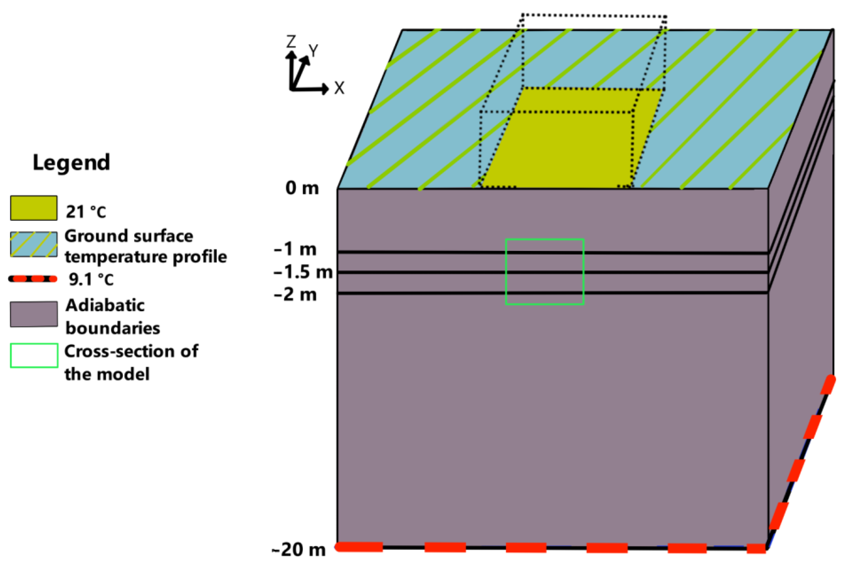
To assess the effect of the greenhouse and its constant temperature at the ground surface on the top of the HGHE, numerical simulations were made for cases with different boundary conditions, representing the presence or absence of the greenhouse above the HGHE.
The outer fluid flow boundaries were treated as no-flow Neumann boundaries. The nodes surrounding the HGHE were also defined as no-flow boundaries to prevent the flow path from leaking. Rain infiltration was considered negligible. The excavations during the fieldwork [23] showed that the groundwater level was below 1.5 m, and the soil was assumed to be unsaturated with water in the shallow ground.
Peripheral heat transfer boundary conditions were defined as adiabatic (Figure 6). Surface temperature varies since some scenarios include a greenhouse above the HGHE, and some do not. The surface covered by the greenhouse was set to have a constant temperature of 21 °C for the simulations, which comes from the Enerprox Inc. study [22]. Otherwise, the surface ground temperature profile (Table 2) was used for the top boundary and an undisturbed ground temperature of 9.1 °C was used for the bottom boundary at a ground depth of 20 m (Figure 6). A given temperature was set at the inlet so that the LFT was known (Figure 7), and the EFT was calculated during the simulations. The LFT was assumed to be −4 °C for the heating and 34 °C for the cooling simulations. However, it should be noted that the chosen LFT values do not accurately represent the hourly energy demand, as it would normally fluctuate through the day.
3.1.6. Initial Conditions and Simulation Time
Prior to the HGHE simulations, numerical models were simulated for a year without any thermal extraction or injection from the HGHE to set the temperature and head values, given that the ground temperature is highly influenced by seasonal temperature variations. In the scenarios where the greenhouse is located above the HGHE, the constant temperature inside the greenhouse (21 °C) is taken into consideration for the initial temperature simulation.
The HGHE simulations were conducted for 5 years, from day 0 to day 1825. The initial time-step length was set to 0.001 days. To ensure optimal results, the minimum time-step size was unrestricted, while the maximum time-step size was set to 5 days. The decision to simulate the model for 5 years allowed us to assess the system’s performance on a long-term basis. The heat pump is assumed to be operating all year for both cooling and heating, and there is going to be either more heat injection or extraction. Simulating the model for only one year would not allow us to observe this effect.
3.2. Coefficient of Performance and Load Coverage Calculations
The coefficient of performance (COP), which is the ratio between the heating power delivered to the building and the electrical power consumed by the heat pump, depends on the EFT and air temperature provided to the building. The coefficient of performance for heating and cooling was calculated using the following equations, according to previous studies [29,30]. A linear formula was used to calculate the COP using tables for commercial ground-source heat pumps and the fluid temperature, varying with time during the simulations. The heating and cooling heat pump COPs were calculated using Equations (8) and (9).
The electrical power consumed by the heat pump (Qc) was calculated using Equations (10) and (11).
where is the ground load (W). The thermal power extracted or injected was calculated using the following equation, which considers the LFT and the EFT, or the temperature at the pipe’s inlet and outlet.
where is the mass flow rate (kg s−1), is the heat capacity (J Kg−1 °C−1) and T is the temperature (°C). The thermal power is averaged monthly for the simulation results. The covered building loads were then calculated by the sum of and in the heating mode and the subtraction of the last two parameters in the cooling mode. The building loads covered by the HGHE were then compared with the total building load profile (Figure 2).
3.3. Simulation Scenarios
Four scenarios were simulated and compared with a base case. In every case, the HGHE covers an area equal to the greenhouse, as shown in Figure 3. The cases referring to the system without a greenhouse imply that the greenhouse is not directly above the system and that it has no impact on the temperature of the soil surrounding the heat exchangers. In this case, the top boundary heat transfer condition was set to the surface ground temperature profile. The cases involving a greenhouse above the system imply that the top boundary condition for heat transfer was set to represent the greenhouse with a constant temperature of 21 °C (Figure 6). In the Base case, there is an HGHE at a 1.5 m depth with no greenhouse above. In Scenario 1, the HGHE is installed at a 1.5 m depth under a greenhouse. In Scenario 2, the HGHE is installed at a 1 m depth under a greenhouse. In Scenario 3, the HGHE is installed at a 2 m depth under a greenhouse. In Scenario 4, a double-layered HGHE is installed at depths of 1 m and 2 m under a greenhouse. Table 5 shows the characteristics of every scenario. Both heating and cooling seasons were simulated.
3.4. Sensitivity Analysis
A sensibility analysis was performed to assess the effect of the surface temperature and ground thermal properties to assess the importance of the building’s localization on the results. The analysis was carried out using the Base case scenario and Scenario 1 numerical model. The ground thermal properties and air temperature were varied to define their effects on the system for each model. The monthly ground surface temperature was increased and decreased by 3 °C, while the ground thermal conductivity and heat capacity values were changed by ±0.345 W m−1 K−1 and ±1.086 MJ m−3 K −1, which represents the maximum and minimum values of the thermal conductivity and heat capacity evaluated for the samples and TRTs made by Géotherma Solutions Inc. [23]. The greenhouse air temperature (21 °C in Scenario 1) always stays the same. Varying input parameters are shown in Table 6.
4. Results
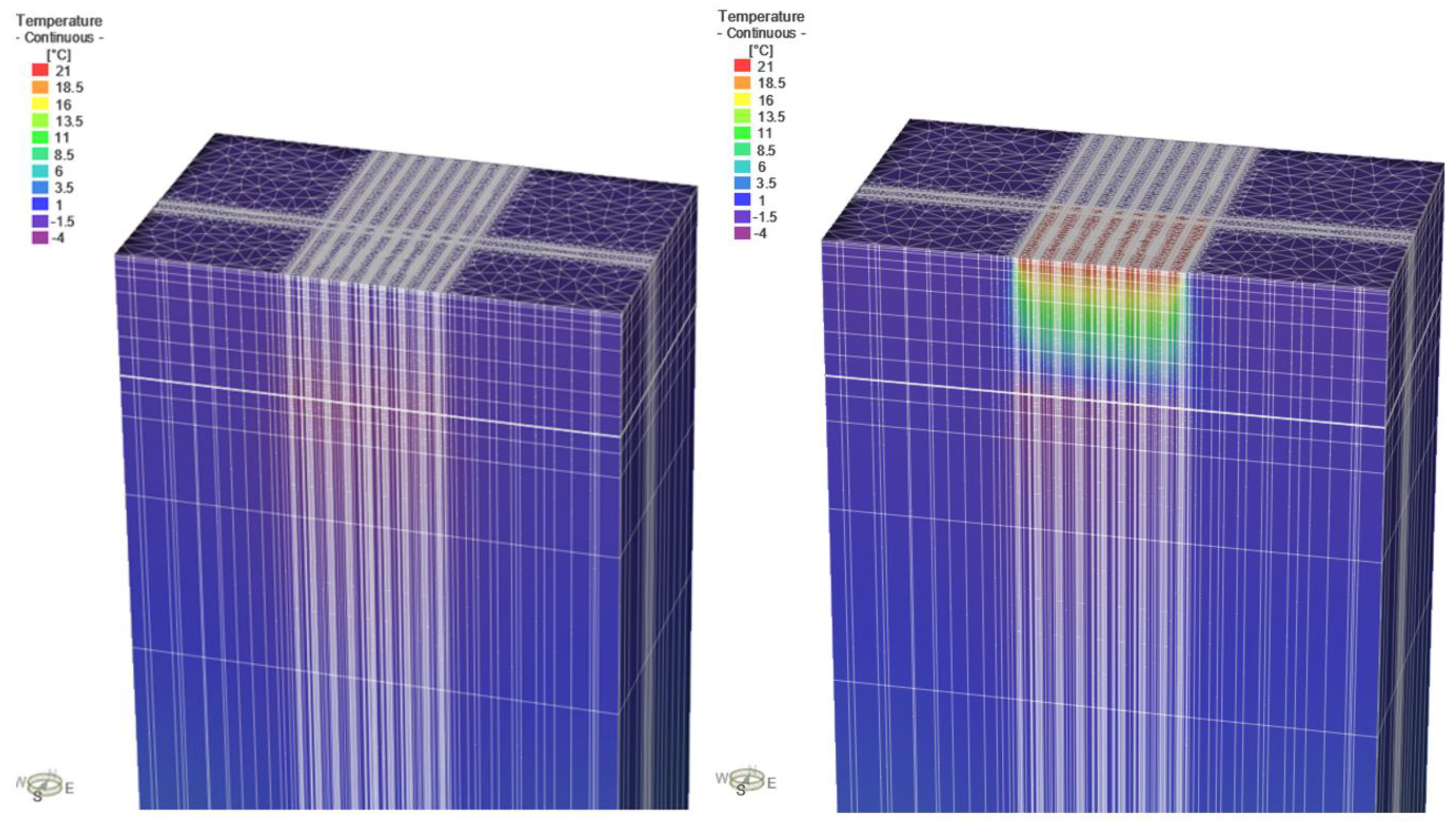
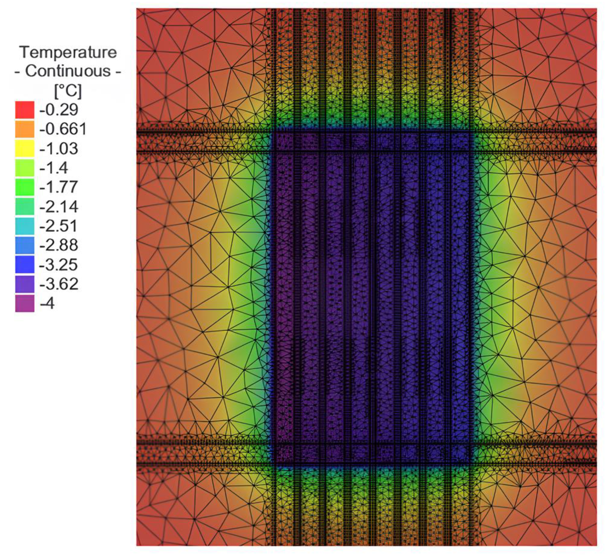
The results for Scenario 1 show that the constant temperature of the greenhouse above the HGHE influences the temperature in the first underground meters (Figure 8 and Figure 9). Here, the constant temperature seems to affect mainly the zone directly below the greenhouse. The results are presented for the months of February and July for both the first and fifth simulation years. February and July represent and will be referred to as the heating and cooling seasons.
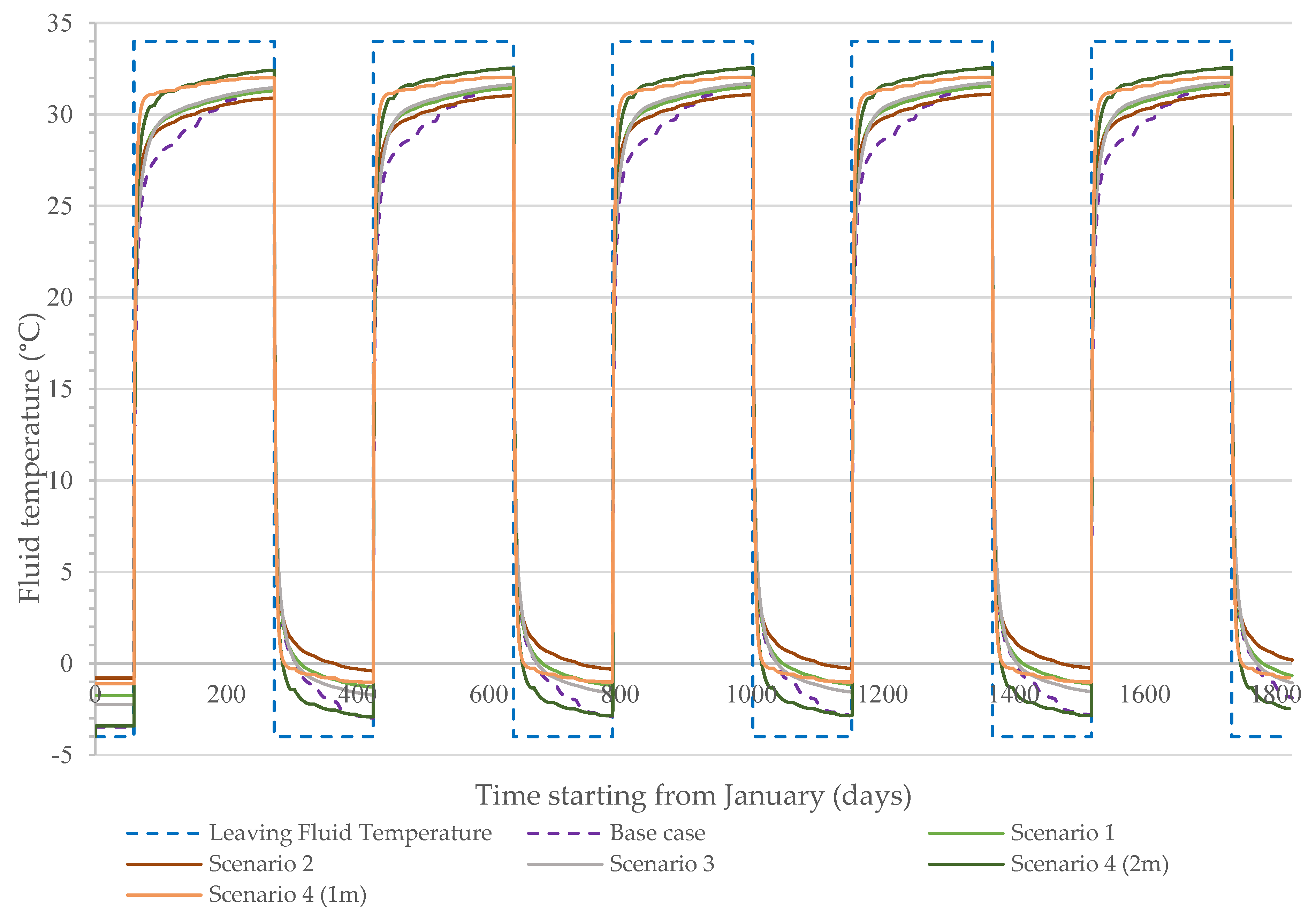
The numerical simulations provide results in the form of fluid temperature for the inlet and the outlet. The following graph shows the EFT for every case, compared with the LFT (Figure 10). The bigger the difference between the EFT and LFT, the better the system’s performance. The LFT (blue line) of 34 °C is for the cooling period, while the LFT of −4 °C is for the heating period.
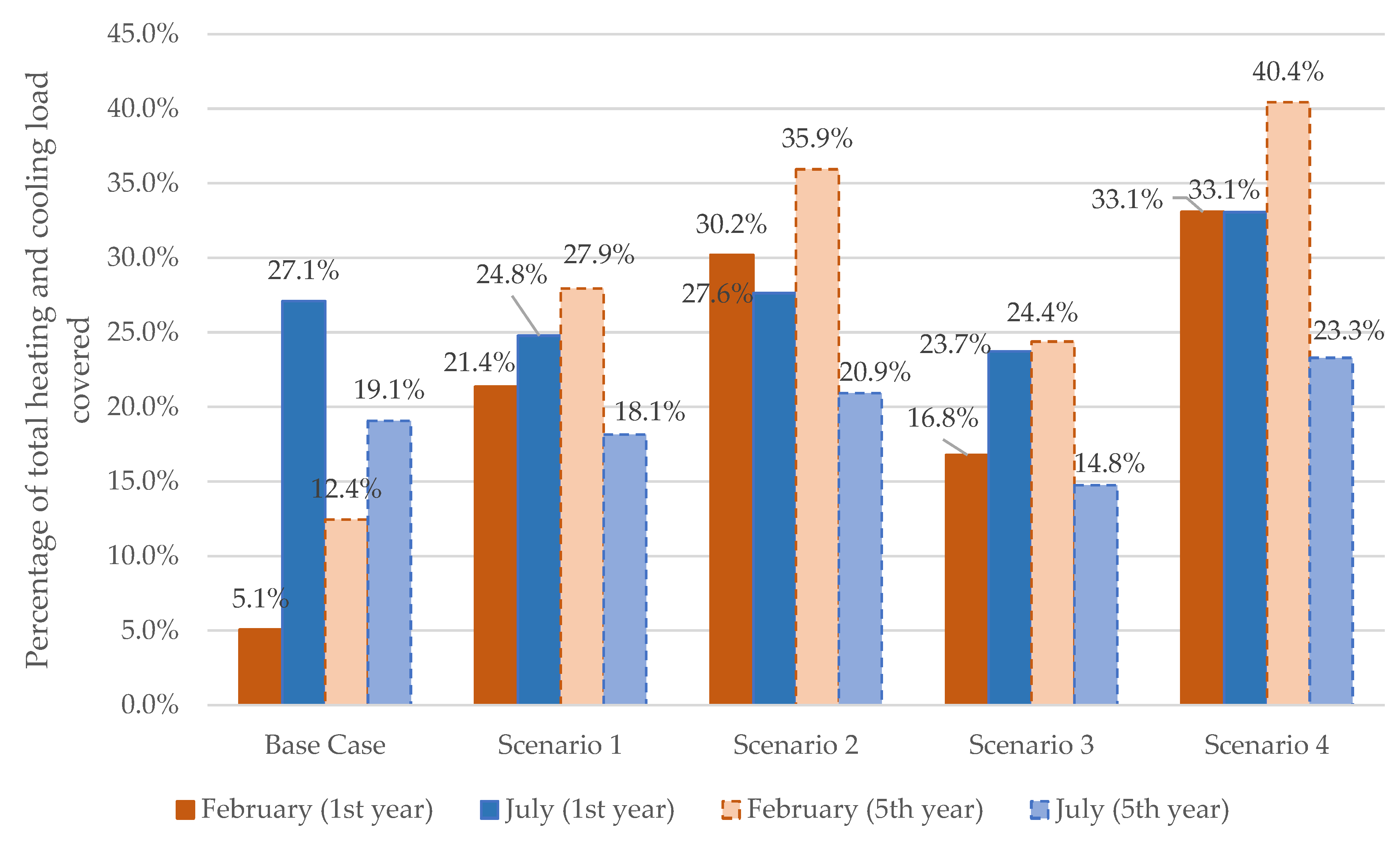
The highest temperature difference between the LFT and EFT during heating periods is observed for Scenario 2, followed by Scenario 1, Scenario 4 (1 m), Scenario 3, Base case and Scenario 4 (2 m). These intermediate results show that the greenhouse has a positive effect on the heating performance. On the other hand, the Base case shows the highest temperature difference during the cooling periods, followed by Scenario 2, Scenario 1, Scenario 3, Scenario 4 (1 m) and Scenario 4 (2 m), which implies that the HGHE is less performant during the cooling periods. The performance of the heat exchanger varies among scenarios at different times of the month. Some scenarios, such as Scenario 4, exhibit a better performance at the beginning of the month, while others perform better toward the end. Hence, evaluating the best scenario based on fluid temperature alone is challenging. To have a better understanding of the results, the fluid temperature can therefore be converted into the percentage of the total heating and cooling covered by the system. The following results focus on the months of February for the heating season and July for the cooling season (Table 7; Figure 11). During the other months, the system covers a higher percentage of the heating and cooling demand.
The COP values shown in Table 7 are higher than the Base case for every scenario in the heating mode, while they are lower in the cooling mode. There is a 0 to 0.18 increase for the month of February, while the values decrease between 0.05 to 0.27 for the month of July when comparing every scenario with the Base case. In the heating mode, Scenario 2 has a higher improvement on the heat pump’s COP. The results show that incorporating a greenhouse structure above the HGHE enhances the heating efficiency while deteriorating the cooling efficiency.
The results for the peak months of February and July demonstrate that the presence of a greenhouse above the HGHE improves the system’s performance for heating but slightly lowers the percentage covered during the cooling phases. The following comparisons between scenarios and the Base case are made for the same year to make the comparisons lighter. Scenario 1 increases the load covered in February by around 15% while it reduces the load covered in June by around 2%. Scenario 2, which implies installing the HGHE at a 1 m depth, increases the load covered in February by 23% to 25% and increases it by 0.5% in July. Scenario 3, which implies installing the HGHE at a depth of 2 m, increases the load covered by around 12% during February while lowers it by 3% during July. Scenario 4, which combines Scenarios 2 and 3, improves both heating and cooling by 28% and 6%, respectively. When looking only at the heating demand, Scenario 4 covers the highest percentage of the total heating load, followed by Scenario 2, Scenario 1, Scenario 3 and the Base case. When looking only at the cooling demand, Scenario 4 covers the highest percentage of the total cooling load, followed by Scenario 2, the Base case, Scenario 1 and Scenario 3. Figure 11 illustrates that the system exhibits better performance in terms of heating during the fifth year, whereas it performs better in terms of cooling during the first year. For the heating season, there is a 6%–8% increase between the first and the fifth years. In contrast, total cooling generally decreases by 8%–10% between the first and fifth years. This can be attributed to a warming ground temperature, either caused by an HGHE unbalanced heat injection versus extraction and temporal propagation of the thermal front from the greenhouse floor toward the subsurface. It can be assumed that the greenhouse constant temperature increases the subsurface temperature over time.
5. Sensitivity Analysis
The COP values are shown for the Base case and for Scenario 1 (Table 8 and Table 9). These tables only display values for the months of February and July, which are representative of the highest and lowest yearly temperatures. It is important to note that the data presented in those tables do not represent the other months.
When compared with the Base case, the results (Table 8) show that raising and reducing ground temperature and changing the ground thermal properties do not significantly impact the COP in the heating mode. There is also no significant change during the first year in the cooling mode. During the fifth year in the cooling mode, raising and lowering the surface ground temperature, respectively, results in 0.44 and −0.03 variations, while deteriorating and enhancing the ground thermal properties results in −0.62 and 0.16 COP variations.
When compared with Scenario 1, the results (Table 9) show that raising and reducing the ground temperature and changing the ground thermal properties do not significantly impact the COP values in the heating mode. There is also no significant change during the first year in the cooling mode. During the fifth year in the cooling mode, raising and lowering the surface ground temperature, respectively, results in 0.66 and 0.01 variations, while deteriorating and enhancing the ground thermal properties results in −0.86 and 0.65 COP variations.
Those results show that, over a prolonged operation period, raising the surface ground temperature as well as reducing and enhancing ground thermal properties has a greater impact on the COP for Scenario 1 compared to the Base case. Since the observed differences are increasing through years of operation, it can be assumed that sustained fluctuations in ambient temperature would be required to impact the system’s performance. The results can also be seen in the form of percentages of the total heating and cooling loads covered by the HGHE (Figure 12 and Figure 13).
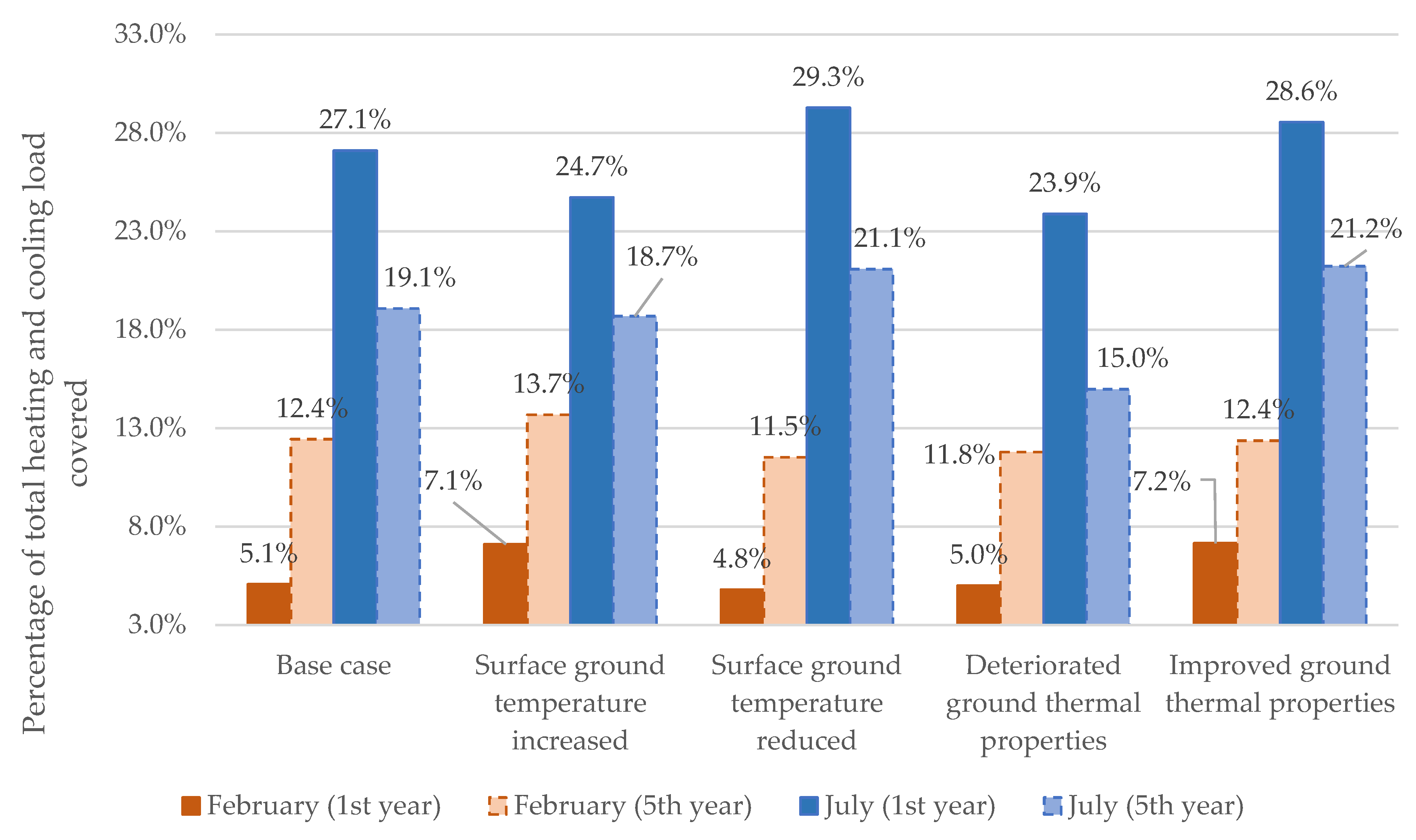
In the Base case (Figure 12), variations in the surface ground temperature and thermal properties have a small impact on load coverage in the heating mode during the first year (−0.3% to 2.1%) and the fifth year (−0.9% to 1.3%). In the cooling mode, variations have a larger impact than in the heating mode during the first (−2.4% to 2.2%) and fifth years (−4% to 2%).
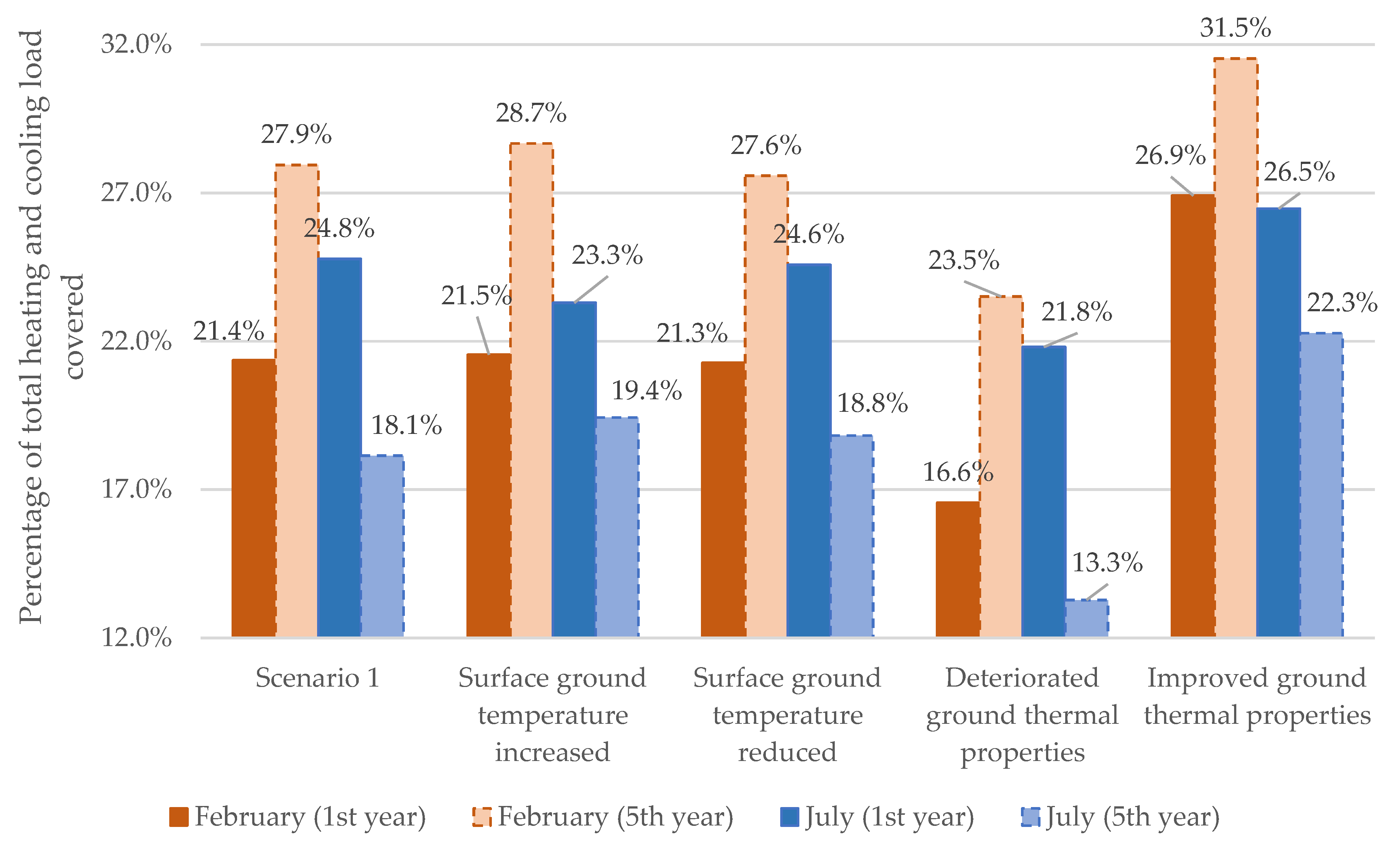
In Scenario 1 (Figure 13), variations in the surface ground temperature have small effects on load coverage during the first year in the heating mode (0.1%) but larger effects during the fifth year (−0.3% to 0.8%). Variations in the ground thermal properties have a more important impact on both the first and the fifth years (−4.8% to 5.5%). In the cooling mode, variations in the surface ground temperature have a smaller effect on both the first and the fifth years (−1.5% to 1.3%), while the thermal properties have a larger impact on both the first and the fifth years (−4.8% to 4.2%).
Those numbers indicate that an ambient temperature has a smaller influence on the system’s performance if a greenhouse with a constant temperature is located above it. In this case, ground thermal properties play an important role in the HGHE’s performance, especially during the cooling phases. In the Base case’s situation, ambient temperature and ground thermal properties are both equally significant.
6. Discussion
This study explores the coupling of greenhouses with HGHEs in a particular context and investigates their heating and cooling performances in urban agriculture. However, these findings may have limited generalizability due to factors such as the short simulation period, constant input parameters, and simplified LFT assumptions. Thus, interpretations of the results should consider the following. Surface water infiltration was not considered; therefore, rain and greenhouse plant watering were assumed to have a negligible impact on the heat transport simulations. The temperature profile used only includes the constant average temperature for every month, which does not represent real-life conditions with hourly fluctuations. The energy consumption monthly values were considered constant according to the energy consumption monthly profile. However, energy consumption varies instantly throughout the day, depending on the building’s energy demand. A simplified LFT was therefore assumed using a constant LFT of −4 °C (heating periods) and 34 °C (cooling periods), while it should vary several times within a day. The model has limitations belonging to its simplifications resulting in assumptions, lack of validation and the homogeneity of the materials. To overcome these limitations, attention should be focused on incorporating more realistic scenarios, validating the models against experimental data, considering a higher range of variables, and addressing the heterogeneity and variability of relevant factors.
In order to make the study and model applicable for worldwide usage, it would be essential to consider a broader range of geographic locations, climate conditions and greenhouse types. Using local data, conducting sensitivity analyses while varying different parameters, assessing economic feasibility and considering the model’s adaptability can make simulations more applicable on a global scale.
This study followed Fujii’s approach [14] using the same pipe diameter for the HGHEs and did not explore alternative HGHE configurations. Fujii et al. [14] developed a specific method tailored to the conditions encountered in their TRT study. However, it is important to note that the parameters they utilized may yield different values when applied to a different soil type. Covering a higher building load with a similar system could be achieved by using thermally improved pipes or reducing the pitch, as Chong et al. [16] indicated. Using pipes with a larger diameter can increase the heat transfer efficiency between the circulating fluid and the ground, as the overall thermal conductivity would increase, and it would be beneficial to the system’s performance.
Fujii’s work [14] was conducted to simulate TRT for a two-week period using a horizontal HGHE, which means that the numerical simulations were only realized for a 2-week time lap. Their work shows that the simulation is well calibrated to the experimental data and that boundary conditions and input parameters are constant with those used in the experiment. Simulating the same system for 5 years can therefore differ from their experiment, given that such a comparison between the numerical and experimental models was not made with different parameters and boundaries. An HGHE simulation for a 5-year period can provide more information on the long-term performance of the system under different environmental conditions; however, small errors or inaccuracies in the model may accumulate over time and result in a deviation from the system’s true behavior. Air temperature, humidity and solar radiation can vary significantly over time; however, this study assumed constant values for these input parameters used in the numerical models.
The purpose of the sensitivity analysis was to assess the system’s response to changes in key parameters and assess their relative importance. We acknowledge that changing the ground thermal properties values may deviate from the conditions under which the model was calibrated. This variation can affect the accuracy of the results and undermine their validity. Therefore, it is essential to interpret the results of the sensitivity analysis with caution. It should be considered as a step towards understanding the behavior of an HGHE system under certain conditions rather than a validation of the model for a larger range of conditions. Future studies should also focus on model validation under a wider range of conditions, including ground thermal properties and ambient temperature.
Installing the system beneath the greenhouse offers several advantages. HGHEs are close to the surface and are impacted by air temperature and seasonal variations. Cold temperatures will increase the viscosity of the propylene glycol/water mixture, thereby reducing thermal conductivity and heat transfer [31]. In cities like Montréal, Québec and La Pocatière, which experience cold winters, the ground temperature near the surface can fall below 0 °C. The inlet fluid temperature, or heat pump LFT, must be lower than the ground temperature to produce heat, which increases the fluid viscosity. Additionally, the fluid can freeze depending on its water proportion. Also, greenhouses are typically constructed on ground level; thus, excavating the area and installing the system directly beneath the structure is easier compared to conventional residential or commercial buildings. This arrangement is also associated with potentially low installation costs.
Our results show that an HGHE with a restricted surface area underneath a greenhouse can provide partial base loads for heating and cooling a greenhouse in a cold continental climate such as Quebec. The different scenarios show that there are strategies to increase the system’s heating efficiency; however, they are still not enough to only rely on the HGHE and the heat pump system. An auxiliary system should be considered in an urban setting, where the area covered by the HGHE is limited, and peak energy demands need to be delivered to the building. Olabi et al. [32] suggested using hybrid geothermal systems, like solar energy systems and cooling towers, coupled with the geothermal system. The former implies that solar collectors, such as photovoltaic thermal hybrid systems, could be used to generate additional heating to cover any deficit from the geothermal system. This would allow the GHE to act as a seasonal energy storage. Such a system is difficult to install on the roof of a greenhouse, as it would prevent the sun from penetrating the building and heating the interior. Otherwise, the coupling of a cooling tower to a geothermal system aims to increase the COP by improving the system’s cooling efficiency with cold water circulation, which allows the hybrid system to maintain a soil thermal balance throughout the year. This type of system can also be coupled with borehole GHEs. Zhou et al. [33] designed a system combining a borehole GHE and an HGHE to reduce the cost of conventional borehole GHE heat pump systems by determining the optimal shape factors, building load distribution scheme and the length of the hybrid GHE.
Géotherma Solutions Inc’s study [23] showed that an HGHE underneath the greenhouse would not provide enough energy to cover the building’s total energy consumption. Using analytical solutions, they showed that the HGHE must be four to nine times greater than the surface area of the greenhouse to do so. This method did not take into consideration the effect of the greenhouse’s constant air temperature on the system’s performance. The ground thermal properties chosen for their studies were also lower when compared to this study. Using sizing calculations, Léveillée-Dallaire et al. [15] showed that 30% to 40% of the heating and cooling peak loads could be covered by an HGHE of the same size as a small greenhouse in Montreal without considering the effect of the greenhouse’s constant temperature. Even though the current study used a numerical approach, the other study’s results are similar to what was obtained in the Base case, which suggests that the system can cover 7.1% of the heating and 26.5% of the cooling loads during the coldest and hottest months. It should be noted that previous studies did not include the effect of the greenhouse above the HGHE.
A comparison between the results for the Base case and Scenario 1 during February and July indicates that installing the HGHE under a greenhouse can double the heating loads covered by the system while slightly lowering the cooling loads covered. This shows that the greenhouse constant temperature has a positive effect on heat extraction. A comparison between scenarios 1, 2 and 3 demonstrates that the closer the system is to the surface (Scenario 2), the better the heat extraction. However, installing a deeper HGHE does not seem to improve either the heating or the cooling performance of the system. Furthermore, Scenario 4 appears to be the best in terms of heating and cooling performance, covering an additional 30% of heating and 6% of cooling compared to the Base case in the short term. Hence, for space optimization, it would be worth choosing this scenario to cover the maximum amount of heating and cooling possible, while further studies need to be completed to evaluate if the extra costs outweigh the system’s benefits.
Between the first and the fifth year of simulation for each scenario, the system’s capacity for heating increases while cooling decreases. In regions with cold climates, heating demand generally outweighs cooling demand, causing the local ground temperature to decrease slightly over time. However, the situation in this study slightly differs and produces contrasting results. The HGHE coupled to a heat pump does not entirely cover the building’s heating and cooling requirements. The objective of this project was to calculate the percentage of a greenhouse’s heating and cooling coverage provided by an HGHE limited in size. As a result, heat production and injection from the HGHE may not follow the building’s consumption needs. Additionally, maintaining a constant temperature in the building could contribute to this increase in the ground temperature over time. Therefore, the incomplete coverage of heating and cooling loads and the building’s constant temperature can create deviations from typical results in cold climates.
The sensitivity analysis indicates that the greenhouse’s constant air temperature reduces the system’s dependence on the ground surface temperature variations for both heating and cooling, even though cooling is less efficient. Hence, there is a notable advantage for heating periods and a small disadvantage for cooling periods. It can therefore be assumed that using such a system has an overall positive effect on the HGHE’s performance in cold regions such as Quebec. The analysis results show the importance of accurately estimating ground thermal properties either by performing a TRT or at least by analyzing ground samples. This shows that a system’s performance can vary according to different types of geological materials and thermal property values. These specific HGHE percentages of total heating and cooling loads covered are obviously expected to differ for HGHEs located in different environments; however, the results can be used as guidelines for greenhouses in a cold continental climate.
7. Conclusions
In conclusion, installing a greenhouse over an HGHE can increase the heating capacity of the system; however, the cooling efficiency tends to decrease. Heating and cooling performances vary according to the depth of the HGHE installation. Additionally, the system had an improved heating performance while the cooling capacity decreased over time, where the HGHE removed heat more efficiently in the cooling phase than during the heating phase. Overall, these results indicate that coupling greenhouses and HGHEs can be an efficient way to improve heating efficiency under some conditions; however, care should be taken to assess their effect on cooling capacity. Considering heating only, Scenario 4 covers the highest percentage of total heating demand between all scenarios, followed by Scenario 2, Scenario 1, Scenario 3 and the Base case.
The sensitivity analysis shows that a change in ground surface temperature affects the system’s performance with increasing operation time, while the ground thermal properties play an important role in the performance of the HGHE, especially during the cooling phases. In addition, ground surface temperature variations seem to play a smaller role in the system’s capacity, with a constant temperature greenhouse located above it when compared to standard HGHEs. The results also indicate the importance of measuring ground thermal properties before installing such a system.
Therefore, the study confirms that a minimum of 7.1% and 26.5% of a small greenhouse’s total heating and cooling loads can be covered in the first year of operation by an HGHE at a 1.5 m depth with no greenhouse above it (Base case). In contrast, installing this same HGHE under a greenhouse with a constant temperature of 21 °C (scenario 1) raises the heating loads covered to 22.8% but decreases the cooling loads covered to 24.2%.
The significance of this study lies in the exploration of coupling greenhouses with HGHEs for improved heating efficiency in urban agriculture. This knowledge is important for urban greenhouse farmers and policymakers seeking sustainable methods to address heating and cooling demands while minimizing energy consumption and costs. Understanding the trade-off between heating and cooling efficiency is essential for decision-making. The insights gained can inform the design of greenhouse-HGHE systems in various urban settings for specific geographic locations.
Following this study, the results could be improved by developing numerical models, including the effect of vertical fluid flow to represent precipitation and/or plant watering, which most likely impacts underground heat transport. Simulations should also be conducted with a complete energy consumption profile, which should be determined hourly to represent the actual heating and cooling demands. An LFT simulation should consider hourly consumption and select temperatures based on the time of day. Further investigations could also explore the economic feasibility of such systems in more standard geographic settings, considering factors such as the system’s maintenance and cost-effectiveness. Future studies could explore the potential of incorporating new numerical models representing different types of HGHEs, such as spiral-coil HGHEs [34] or cylindrical-finned HGHEs [35].
Author Contributions
Conceptualization, X.L.-D. and J.R.; Methodology, X.L.-D. and J.R.; Software, X.L.-D., J.R. and H.F.; Formal analysis, X.L.-D.; Writing – original draft, X.L.-D.; Writing – review & editing, X.L.-D., J.R., J.Þ.S., H.F. and H.L.; Supervision, J.R. and H.F.; Project administration, J.R.; Funding acquisition, J.R. All authors have read and agreed to the published version of the manuscript.
Funding
This research was carried out under the Communoserre project funded by INRS with a special grant for research on the COVID-19 pandemic and its impact on society.
Data Availability Statement
The different FEFLOW models created and simulated, as well as the tables regrouping all the simulation results, are available online and can be accessed through the Boréalis website (https://borealisdata.ca/). To access the files, one must simply search the DOI https://doi.org/10.5683/SP3/IJFGG9.
Conflicts of Interest
The authors declare no conflict of interest.
References
- McClintock, N. Why farm the city? Theorizing urban agriculture through a lens of metabolic rift. Camb. J. Reg. Econ. Soc. 2010, 3, 191–207. [Google Scholar] [CrossRef] [Green Version]
- Gundersen, C.; Hake, M.; Dewey, A.; Engelhard, E. Food Insecurity during COVID-19. Appl. Econ. Perspect. Policy 2021, 43, 153–161. [Google Scholar] [CrossRef] [PubMed]
- Lund, E.M.; Forber-Pratt, A.J.; Wilson, C.; Mona, L.R. The COVID-19 pandemic, stress, and trauma in the disability community: A call to action. Rehabil. Psychol. 2020, 65, 313–322. [Google Scholar] [CrossRef]
- Mok, H.-F.; Williamson, V.G.; Grove, J.R.; Burry, K.; Barker, S.F.; Hamilton, A.J. Strawberry fields forever? Urban agriculture in developed countries: A review. Agron. Sustain. Dev. 2014, 34, 21–43. [Google Scholar] [CrossRef] [Green Version]
- Schupp, J.L. Cultivating Better Food Access? The Role of Farmers’ Markets in the U.S. Local Food Movement. Rural Sociol. 2017, 82, 318–348. [Google Scholar] [CrossRef]
- Bach, C.E.; McClintock, N. Reclaiming the city one plot at a time? DIY garden projects, radical democracy, and the politics of spatial appropriation. Environ. Plan. C Polit. Space 2021, 39, 859–878. [Google Scholar] [CrossRef]
- Ahamed, M.S.; Guo, H.; Tanino, K. Energy saving techniques for reducing the heating cost of conventional greenhouses. Biosyst. Eng. 2019, 178, 9–33. [Google Scholar] [CrossRef]
- Mohamed, M.B. Geothermal resource development in agriculture in Kebili region, Southern Tunisia. Geothermics 2003, 38, 392–398. [Google Scholar] [CrossRef]
- Zhang, S.; Guo, Y.; Zhao, H.; Wang, Y.; Chow, D.; Fang, Y. Methodologies of control strategies for improving energy efficiency in agricultural greenhouses. J. Clean. Prod. 2020, 274, 122695. [Google Scholar] [CrossRef]
- IPCC. Summary for Policy Makers: Working Group 11 Contribution to the Fifth Assessment Report of the Intergovernmental Panel on Climate Change; Public Report; Cambridge University Press: Cambridge, MA, USA, 2014; pp. 1–32. Available online: https://www.ipcc.ch/report/ar5/syr/ (accessed on 23 December 2021).
- De Rosa, M.; Gainsford, K.; Pallonetto, F.; Finn, D.P. Diversification, concentration and renewability of the energy supply in the European Union. Energy 2022, 253, 124097. [Google Scholar] [CrossRef]
- Farabi-Asl, H.; Fujii, H.; Kosukegawa, H. Cooling tests, numerical modeling and economic analysis of semi-open loop ground source heat pump system. Geothermics 2018, 71, 34–45. [Google Scholar] [CrossRef]
- Fujii, H.; Yamasaki, S.; Maehara, T.; Ishikami, T.; Chou, N. Numerical simulation and sensitivity study of double-layer Slinky-coil horizontal ground heat exchangers. Geothermics 2013, 47, 61–68. [Google Scholar] [CrossRef]
- Fujii, H.; Nishi, K.; Komaniwa, Y.; Chou, N. Numerical modeling of slinky-coil horizontal ground heat exchangers. Geothermics 2012, 41, 55–62. [Google Scholar] [CrossRef]
- Léveillée-Dallaire, X.; Raymond, J.; Fujii, H.; Tsuya, S. Sizing Horizontal Geothermal Heat Exchangers for Community Greenhouses in Montreal. In Proceedings of the 2022 Geothermal Rising Conference: Using the Earth to Save the Earth, GRC 2022, Reno, NV, USA, 28–31 August 2022; INRS—Centre Eau Terre Environnement: Quebec City, QC, Canada, 2022. Chapter 46. pp. 793–803. [Google Scholar]
- Chong, C.S.A.; Gan, G.; Verhoef, A.; Garcia, R.G.; Vidale, P.L. Simulation of thermal performance of horizontal slinky-loop heat exchangers for ground source heat pumps. Appl. Energy 2013, 104, 603–610. [Google Scholar] [CrossRef]
- Tang, F.; Nowamooz, H. Outlet temperatures of a slinky-type Horizontal Ground Heat Exchanger with the atmosphere-soil interaction. Renew. Energy 2020, 146, 705–718. [Google Scholar] [CrossRef]
- Larwa, B.; Teper, M.; Grzywacz, R.; Kupiec, K. Study of a slinky-coil ground heat exchanger—Comparison of experimental and analytical solution. Int. J. Heat Mass Transf. 2019, 142, 118438. [Google Scholar] [CrossRef]
- Wu, Y.; Gan, G.; Verhoef, A.; Vidale, P.L.; Gonzalez, R.G. Experimental measurement and numerical simulation of horizontal-coupled slinky ground source heat exchangers. Appl. Therm. Eng. 2010, 30, 2574–2583. [Google Scholar] [CrossRef] [Green Version]
- Xing, L.; Cullin, J.R.; Spitler, J.D. Modeling of foundation heat exchangers—Comparison of numerical and analytical approaches. Build. Simul. 2012, 5, 267–279. [Google Scholar] [CrossRef]
- Diersch, H.-J.G. FEFLOW: Finite Element Modeling of Flow, Mass and Heat Transport in Porous and Fractured Media; Springer Science & Business Media: Berlin/Heidelberg, Germany, 2013; ISBN 978-3-642-38739-5. [Google Scholar]
- Enerprox. Biopterre Study Summary; Confidential Report; Enerprox: Victoriaville, QC, Canada, 2022. (In French) [Google Scholar]
- Géotherma Solutions Inc. Pre-Feasibility Study of a Forced-Air Geothermal System to Heat and Cool a Research Building to Be Built in Sainte-Anne-de-la-Pocatière, Quebec; Preliminary Report—Confidential; Géotherma Solutions Inc.: Quebec City, QC, Canada, 2022. (In French) [Google Scholar]
- Langevin, H.; Giordano, N.; Raymond, J.; Gosselin, L. Oscillatory thermal response test using heating cables: A novel method for in-situ thermal property analysis. Int. J. Heat Mass Transf. 2023, 202, 123646. [Google Scholar] [CrossRef]
- Ouzzane, M.; Eslami-Nejad, P.; Badache, M.; Aidoun, Z. New correlations for the prediction of the undisturbed ground temperature. Geothermics 2015, 53, 379–384. [Google Scholar] [CrossRef]
- Government of Canada. (n.d.). Canadian Climate Normals 1981–2010 Station Data for Montréal/Pierre Elliott Trudeau International Airport. Canada. Available online: https://climat.meteo.gc.ca/climate_normals/results_f.html?searchType=stnName&txtStationName=la+poca&searchMethod=contains&txtCentralLatMin=0&txtCentralLatSec=0&txtCentralLongMin=0&txtCentralLongSec=0&stnID=5806&dispBack=1 (accessed on 13 December 2021).
- Langevin, H. Investigation of Ground-Source Heat Pump and Underground Thermal Storage Systems in the Nordic Region: Subsurface Aspects. Master’s Thesis, INRS—Centre Eau Terre Environnement, Quebec City, QC, Canada, 2022. (In French). [Google Scholar]
- Léveillée-Dallaire, X.; Comeau, F.-A.; Raymond, J. Evaluation of the Geothermal Potential of Hybrid Heat Exchangers: Semi-Open Vertical Loop with Well Groundwater Convection; Technical report No. I426. Issue I426; INRS—Centre Eau, Terre et Environnement: Quebec City, QC, Canada, 2020; Available online: https://espace.inrs.ca/id/eprint/11752/ (accessed on 12 October 2022). (In French)
- Casasso, A.; Sethi, R. Efficiency of closed loop geothermal heat pumps: A sensitivity analysis. Renew. Energy 2014, 62, 737–746. [Google Scholar] [CrossRef] [Green Version]
- Hein, P.; Kolditz, O.; Görke, U.-J.; Bucher, A.; Shao, H. A numerical study on the sustainability and efficiency of borehole heat exchanger coupled ground source heat pump systems. Appl. Therm. Eng. 2016, 100, 421–433. [Google Scholar] [CrossRef]
- Hydrosolar Why and When Horizontal Geothermal Fail to Deliver Energy Savings. Advanced Technical Zone. Available online: https://hydrosolar.ca/blogs/advanced-technical-zone/why-and-when-horizontal-geothermal-fail-to-deliver-energy-savings (accessed on 22 February 2022).
- Olabi, A.G.; Mahmoud, M.; Soudan, B.; Wilberforce, T.; Ramadan, M. Geothermal based hybrid energy systems, toward eco-friendly energy approaches. Renew. Energy 2020, 147, 2003–2012. [Google Scholar] [CrossRef]
- Zhou, K.; Mao, J.; Li, Y.; Zhang, H.; Chen, S.; Chen, F. Thermal and economic performance of horizontal ground source heat pump systems with different flowrate control methods. J. Build. Eng. 2022, 53, 104554. [Google Scholar] [CrossRef]
- Kim, M.-J.; Lee, S.-R.; Yoon, S.; Jeon, J.-S. An applicable design method for horizontal spiral-coil-type ground heat exchangers. Geothermics 2018, 72, 338–347. [Google Scholar] [CrossRef]
- Saeidi, R.; Noorollahi, Y.; Chang, S.; Yousefi, H. A comprehensive study of Fin-Assisted horizontal ground heat exchanger for enhancing the heat transfer performance. Energy Convers. Manag. X 2023, 18, 100359. [Google Scholar] [CrossRef]
Figure 1.
La Pocatière greenhouse location shown by a red star (ESRI, UTM Zone 19N).

Figure 2.
Monthly heating and cooling load profile evaluated for the greenhouse in La Pocatière [22].
Figure 2.
Monthly heating and cooling load profile evaluated for the greenhouse in La Pocatière [22].

Figure 3.
Concept of the study’s model.

Figure 4.
3D view of the numerical model showing the HGHE (green filled area).

Figure 5.
Excerpt from Figure 4 representing a cross-section of the thin plate model. Blue: flow path. Gray: pipe walls.
Figure 5.
Excerpt from Figure 4 representing a cross-section of the thin plate model. Blue: flow path. Gray: pipe walls.

Figure 6.
Model heat transfer boundary conditions for simulations at different depths. A cross-section is shown in Figure 7.
Figure 6.
Model heat transfer boundary conditions for simulations at different depths. A cross-section is shown in Figure 7.

Figure 7.
The middle slice of the HGHE model (Figure 5) and the key internal conditions used to simulate HGHEs. The Well BC injection and pumping refer to fluid injection and extraction at the beginning and the end of the HGHE, respectively.
Figure 7.
The middle slice of the HGHE model (Figure 5) and the key internal conditions used to simulate HGHEs. The Well BC injection and pumping refer to fluid injection and extraction at the beginning and the end of the HGHE, respectively.

Figure 8.
Cross-section of the numerical model’s temperature in January. (Left), Base case. (Right), Scenario 1.
Figure 8.
Cross-section of the numerical model’s temperature in January. (Left), Base case. (Right), Scenario 1.

Figure 9.
Slice view of a numerical simulation showing the HGHE at a 1.5 m depth.

Figure 10.
Fluid temperature for every simulation scenario.

Figure 11.
Heating and cooling loads covered for February and July.

Figure 12.
Base case—sensitivity analysis results for February and July.

Figure 13.
Scenario 1—sensitivity analysis results for February and July.


Table 1.
Ground thermal properties.
| Samples | OTRT | Chosen Value | |
|---|---|---|---|
| (Géotherma Solutions Inc.) | (Géotherma Solutions Inc.) | ||
| Ground heat capacity (MJ m−3 K−1) | 2.85–4.05 | 1.78–2.62 | 2.86 |
| Ground thermal conductivity (W m−1 K−1) | 1.45–1.50 | 1.07–1.60 | 1.41 |
Table 2.
Ground surface temperature profile.
| Months | Ambient Temperature Tamb (°C) | Calculated Ground Surface Temperature Tgs (°C) | Ground Surface Temperature Tgs Considering Snow Isolation (°C) |
|---|---|---|---|
| January | −11.6 | −6.5 | −1.0 |
| February | −9.4 | −4.4 | −1.0 |
| March | −4.0 | 0.7 | 0.7 |
| April | 3.7 | 8.0 | 8.0 |
| May | 11.2 | 15.2 | 15.2 |
| June | 15.9 | 19.6 | 19.6 |
| July | 18.8 | 22.4 | 22.4 |
| August | 18.5 | 22.1 | 22.1 |
| September | 13.9 | 17.7 | 17.7 |
| October | 6.9 | 11.1 | 11.1 |
| November | 0.5 | 5.0 | 5.0 |
| December | −7.2 | −2.3 | −1.0 |
Table 3.
Operating parameters.
| HGHE Parameters | |
|---|---|
| HGHE pitch (m) | 0.6 |
| HGHE slinky-coil diameter (m) | 0.8 |
| HGHE pipe thermal conductivity (W m−1 K−1) | 0.34 |
| Inner pipe diameter (m) | 0.024 |
| Outer pipe diameter (m) | 0.034 |
| Flow rate (m d−1) | 17 |
| Fluid composition (% of propylene glycol) | 20 |
| Fluid freezing point (°C) | −7.1 |
| Fluid heat capacity (MJ m−3 K−1) | 4.02 |
Table 4.
Model properties.
| Flow Path | Pipes | Ground | ||
|---|---|---|---|---|
| Hydraulic properties | Hydraulic conductivity (m s−1) | 0.001 | 1.00 × 10⁻¹⁵ | 1.00 × 10⁻¹⁵ |
| Porosity | 1 | 0.0001 | 0.0001 | |
| Thermal properties | Heat capacity (MJ m−1 K−1) | 3.800 | 2.86 | 2.86 |
| Thermal conductivity (W m−3 K−1) | 0.027 | 0.027 | 1.414 |
Table 5.
Characteristics of every scenario.
| Depth of the HGHE (m) | Presence of Greenhouse Above the System | Surface Ground Temperature Above the System | Number of HGHE Layers | |
|---|---|---|---|---|
| Base Case | 1.5 | No | Ground surface temperature profile | 1 |
| Scenario 1 | 1.5 | Yes | 21 °C | 1 |
| Scenario 2 | 1 | Yes | 21 °C | 1 |
| Scenario 3 | 2 | Yes | 21 °C | 1 |
| Scenario 4 | 1 and 2 | Yes | 21 °C | 2 |
Table 6.
Varied input parameters for the sensitivity analysis.
| Ground Surface Temperature for Every Month (°C) | Ground Thermal Conductivity (W m−1 K−1) | Ground Heat Capacity (MJ m−3 K −1) | |
|---|---|---|---|
| Base case | 0 | 1.414 | 2.860 |
| Surface ground temperature increased | +3 | 1.414 | 2.860 |
| Surface ground temperature reduced | −3 | 1.414 | 2.860 |
| Deteriorated ground thermal properties | 0 | 1.069 | 3.946 |
| Improved ground thermal properties | 0 | 1.758 | 1.774 |
Table 7.
COP calculated for February and July from LFT.
| Base Case | Scenario 1 | Scenario 2 | Scenario 3 | Scenario 4 | |
|---|---|---|---|---|---|
| February (1st year) | 3.78 | 3.88 | 3.96 | 3.84 | 3.80 |
| February (5th year) | 3.80 | 3.90 | 3.98 | 3.87 | 3.80 |
| July (1st year) | 6.90 | 6.79 | 6.85 | 6.77 | 6.63 |
| July (5th year) | 6.84 | 6.74 | 6.58 | 8.65 | 6.60 |
Table 8.
Base case—sensitivity analysis COP values for February and July.
| Base Case | Surface Ground Temperature Increased | Surface Ground Temperature Reduced | Deteriorated Ground Thermal Properties | Improved Ground Thermal Properties | |
|---|---|---|---|---|---|
| February (first year) | 3.62 | 3.64 | 3.63 | 3.63 | 3.64 |
| February (fifth year) | 3.69 | 3.70 | 3.68 | 3.68 | 3.69 |
| July (first year) | 6.79 | 6.75 | 6.84 | 6.73 | 6.82 |
| July (fifth year) | 5.19 | 5.63 | 5.20 | 4.57 | 5.35 |
Table 9.
Scenario 1—sensitivity analysis COP values for February and July.
| Scenario 1 | Surface Ground Temperature Increased | Surface Ground Temperature Reduced | Deteriorated Ground Thermal Properties | Improved Ground Thermal Properties | |
|---|---|---|---|---|---|
| February (first year) | 3.78 | 3.78 | 3.78 | 3.73 | 3.84 |
| February (fifth year) | 3.85 | 3.85 | 3.84 | 3.80 | 3.88 |
| July (first year) | 6.75 | 6.72 | 6.75 | 6.69 | 6.78 |
| July (fifth year) | 5.46 | 6.12 | 5.47 | 4.60 | 6.11 |
Disclaimer/Publisher’s Note: The statements, opinions and data contained in all publications are solely those of the individual author(s) and contributor(s) and not of MDPI and/or the editor(s). MDPI and/or the editor(s) disclaim responsibility for any injury to people or property resulting from any ideas, methods, instructions or products referred to in the content. |
© 2023 by the authors. Licensee MDPI, Basel, Switzerland. This article is an open access article distributed under the terms and conditions of the Creative Commons Attribution (CC BY) license (https://creativecommons.org/licenses/by/4.0/).
Share and Cite
MDPI and ACS Style
Léveillée-Dallaire, X.; Raymond, J.; Snæbjörnsson, J.Þ.; Fujii, H.; Langevin, H. Performance Assessment of Horizontal Ground Heat Exchangers under a Greenhouse in Quebec, Canada. Energies 2023, 16, 5596. https://doi.org/10.3390/en16155596
AMA Style
Léveillée-Dallaire X, Raymond J, Snæbjörnsson JÞ, Fujii H, Langevin H. Performance Assessment of Horizontal Ground Heat Exchangers under a Greenhouse in Quebec, Canada. Energies. 2023; 16(15):5596. https://doi.org/10.3390/en16155596
Chicago/Turabian StyleLéveillée-Dallaire, Xavier, Jasmin Raymond, Jónas Þór Snæbjörnsson, Hikari Fujii, and Hubert Langevin. 2023. "Performance Assessment of Horizontal Ground Heat Exchangers under a Greenhouse in Quebec, Canada" Energies 16, no. 15: 5596. https://doi.org/10.3390/en16155596
Note that from the first issue of 2016, this journal uses article numbers instead of page numbers. See further details here.