
Experimental Study of the Transient Behavior of a Wind Turbine Wake Following Yaw Actuation


1
Department of Engineering Mechanics, KTH Royal Institute of Technology, 11428 Stockholm, Sweden
2
Department of Earth Sciences, Uppsala University, 75236 Uppsala, Sweden
*
Author to whom correspondence should be addressed.
Energies 2023, 16(13), 5147; https://doi.org/10.3390/en16135147
Submission received: 10 June 2023
/
Revised: 29 June 2023
/
Accepted: 30 June 2023
/
Published: 4 July 2023
(This article belongs to the Section A3: Wind, Wave and Tidal Energy)
Abstract
:Wind tunnel experiments were performed to investigate the response of a wind turbine model immersed in a replicated atmospheric boundary layer to dynamic changes in the yaw angle. Both the flow field in the wake and the operating properties of the turbine, namely its thrust force, torque, and angular velocity, were monitored during repeated yaw maneuvers for a variety of yaw angles. It was observed that the characteristic time scale of the transient experienced by the turbine scalar quantities was one order of magnitude larger than that of the yaw actuation and depended primarily on the inertia of the rotor and the generator. Furthermore, a Morlet wavelet analysis of the thrust signal showed a strong peak at the rotation frequency of the turbine, with the transient emergence of high activity at a lower frequency during the yaw maneuver. The insights provided by the proper orthogonal decomposition analysis performed on the wake velocity data enabled the development of a simple reduced-order model for the transient in the flow field based on the stationary states before and after the yaw maneuver. This model was then further improved to require only the final state, extending its applicability to any arbitrary wind farm as a dynamical surrogate of the farm behavior.
1. Introduction
In recent years, the role played by wind energy in the global energy budget has grown significantly, and this trend is expected to continue in the future [1]. The increase in the number of installed wind plants has highlighted the importance of finding optimal methods for their operation [2], with the aim of reducing fatigue loads [3,4], thus extending the structural life span, and maximising the power output, for example by means of wake-steering control strategies [5,6]. Modern wind turbines are affected by the local properties of the atmospheric boundary layer (ABL), which can trigger unsteady wake motions in response to approaching eddies [7]. Floating offshore turbines are also influenced by the wave-induced motion of their platforms [8]. These environmental conditions are characterized by stochastic changes across a vast range of time scales. This entails that the optimal management of a wind farm requires a robust understanding of the turbines’ dynamic response to these external phenomena.
Tobin and Chamorro [9] showed how power fluctuations depend on the incoming flow properties. Starting from the equation for the energy budget, they were able to find the transfer function between the power spectrum of the generated power and the flow field. They showed that turbines are not influenced by length scales smaller than their diameter, while larger scales affect turbines nonlinearly. A simplified model was also proposed, wherein the turbine was treated as a Butterworth filter. Later, Zhang et al. [10] performed a similar study on the modulation of the pitching and rolling motions (typical of a floating turbine) by the frequency spectrum of the incoming wind.
The recent interest in control strategies involving wake steering has led to the development of analytical wake models capable of predicting the wake deflection induced by yaw angle misalignment [11,12]. These steady-state models, however, do not capture the downstream propagation of the changes occurring in the wake as a result of yawing maneuvers, nor the velocity adjustment times. They assume instead that the flow field is modified instantaneously. Advanced control strategies should take this time dependence into account when computing real-time optimal farm configurations and therefore implement dynamic wake models. An example is the FLORIDyn model [13,14], which adopts a Lagrangian approach with observation points traveling with the flow along the wake centerline and carrying the information related to the state of the turbine. This model is capable of responding dynamically to changes in the yaw angle. Recently, Foloppe et al. [15] devised a revision of FLORIS [16] (the underlining model used in FLORIDyn) and studied both mesoscale and frontal changes in wind direction. Another recent model combined flow sensing around turbines and a wake model to obtain real-time corrections to flow-field predictions [17].
A key requirement of such models is that they must be computationally fast in order to instantaneously determine the optimal farm configuration given the current environmental conditions. Higher-fidelity simulations are not suited for real-time operations but can provide further insights into the mechanisms underlying the wake response. Ebrahimi and Sekandari [18] studied the transient response to sudden wind gusts and yaw angle changes using a vortex lattice method combined with structural simulations. They showed that the responses of thrust, power, and blade deflection to yaw maneuvers had the same duration. Abraham et al. [19] performed large eddy simulations (LES) to study the wake modulation caused by ramp-like changes in the blade pitch angle and the turbine yaw. In the latter case, they observed a transient wake deflection in the opposite direction to the deflection observed for steady-state conditions. This transient deflection was most evident in the near wake and decreased in magnitude as it traveled downstream. The authors proposed that it was caused by a temporary imbalance in streamwise vorticity occurring during the yawing maneuver.
Experimental studies can provide valuable insights into the dynamic responses of wind turbines, most notably when transitions take place in controlled conditions, as is the case in wind tunnel experiments. Yu et al. [20] recently performed a wind tunnel study on the effect of unsteady loading on the wake of a porous disc. Similarly, Macrì et al. [21] conducted wind tunnel experiments examining an actuator disc’s response to yawing maneuvers. They examined the transient of the wake deflection and the dynamic loads experienced by a second disc located downstream. They showed that the duration of the yawing maneuver was similar to that of the wake deflection adjustment, but longer than that of the dynamic load change at the downstream turbine. They also observed asymmetry in the time scales between the turbine misalignment and realignment with the wind. Field experiments can also prove highly valuable, because the multitude of stochastic changes in the flow conditions experienced by full-scale turbines are difficult to reproduce in a wind tunnel. In this regard, Abraham and Hong [22] recently demonstrated the importance of the dynamic wake modulation caused by constantly changing inflow conditions on the wake recovery of a 2.5 MW turbine.
In this work, we extended the analysis of the dynamic response of a small-scale turbine model to yawing maneuvers by means of wind tunnel experiments. The wake of a three-bladed rotor, along with its thrust force and power production, was studied during rapid rotations to different yaw angles. Furthermore, the velocity field was analyzed by means of the proper orthogonal decomposition (POD) technique, so that a simple reduced-order model that described the evolution of the velocity field over time was developed. This paper is organized as follows: The description of the experimental facility, wind turbine model, and procedures used for data acquisition are presented in Section 2. The analysis of the wake and turbine scalar quantities (namely its torque, thrust, and angular velocity) are presented in Section 3. This section also includes the POD analysis of the velocity field. A simple reduced-order model for modeling unsteady wake behavior that can be extended to arbitrary wind farms is presented in Section 4. The final remarks are contained in Section 5.
2. Materials and Methods
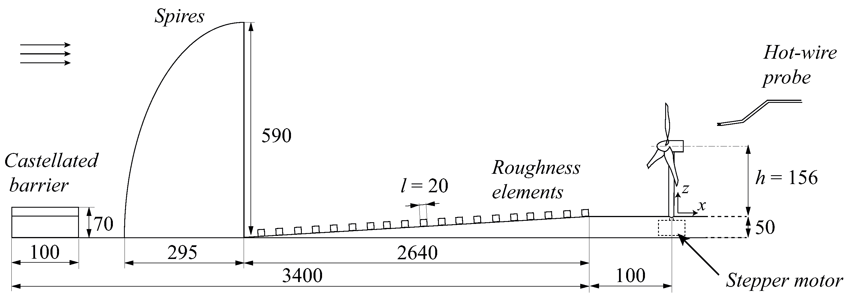
The experiments were conducted in the minimum turbulence level (MTL) wind tunnel at the KTH Royal Institute of Technology. The test section of this closed-loop facility is long and has a cross-section of . The temperature in the tunnel can be regulated within ±0.05 °C by means of a heat exchanger located in the return circuit. A complete characterization of the tunnel can be found in Lindgren and Johansson’s work [23]. The thickness of the boundary layer that developed naturally on the tunnel floor was not sufficient to engulf the turbine model, given the limited length of the test section. An atmospheric boundary layer was therefore artificially replicated by means of the Counihan method [24]. This entailed mounting a castellated barrier at the inlet of the test section, followed by vortex generators and then by a roughness fetch. The seven vortex generators used in this work were tall, and their design was based on the recommendations of Hohman et al. [25] to maximize the degree of span-wise homogeneity of the resulting boundary layer. The roughness fetch was long and consisted of wooden cubes with sides arranged in staggered rows separated by a distance of in the stream-wise direction. The distance between cubes within a row was , and the span-wise offset between rows was . In addition, foam panels were placed in the test section, acting as the effective floor. Their thickness increased linearly from downstream of the vortex generators to at the end of the roughness fetch and remained constant thereafter. Furthermore, the ceiling of the test section was adjusted to provide a pressure gradient of zero within the measurement region. A schematic representation of the experimental setup is shown in Figure 1.
The velocity measurements were performed with hot-wire anemometry. The characterization of the ABL was carried out with a single-wire hot-wire probe, whose platinum–rhodium wire was long and had a diameter of . The wake of the turbine was instead studied with an X-wire probe, consisting of two platinum wires with a diameter of and length of . This probe could be rotated by 90° so that the stream-wise velocity could be measured together with either the vertical or lateral component. The probes were mounted onto an long sting, which was in turn connected to a 3-axis traverse system. The daily calibration of the probes was carried out using a Prandtl tube mounted on the ceiling of the test section in the case of the single wire and a calibration jet apparatus in the case of the X-wire.
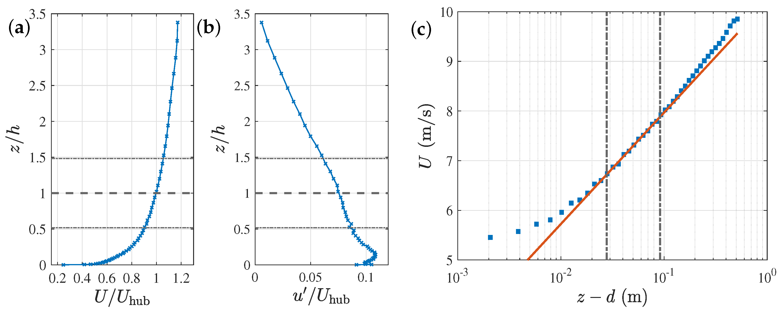
The experiments were conducted with a free-stream velocity above the edge of the boundary layer of , resulting in a velocity at hub height of . The vertical profiles of the mean and standard deviation of the stream-wise velocity component , normalized with , are presented in Figure 2a,b, respectively. The stream-wise turbulence intensity at hub height was , and the thickness of the ABL, defined as the distance from the wall where the local velocity reached of , was . The fact that was smaller than the height of the vortex generators was most likely due to the combination of foam panels and the weakening finite-end effect of the spires. Figure 2c shows a logarithmic law in the form fitted to the experimental data within the vertical interval defined by , where is the height of the roughness elements. This restriction is meant to exclude the roughness sublayer as well as the turbulent boundary layer wake from the fit [26]. The friction velocity obtained with the von Kármán constant [27] is , the displacement height is , and the roughness length is . Furthermore, a power law was fitted to the same z interval, resulting in a shear exponent , which is associated with an ABL over a flat terrain with low vegetation [28].
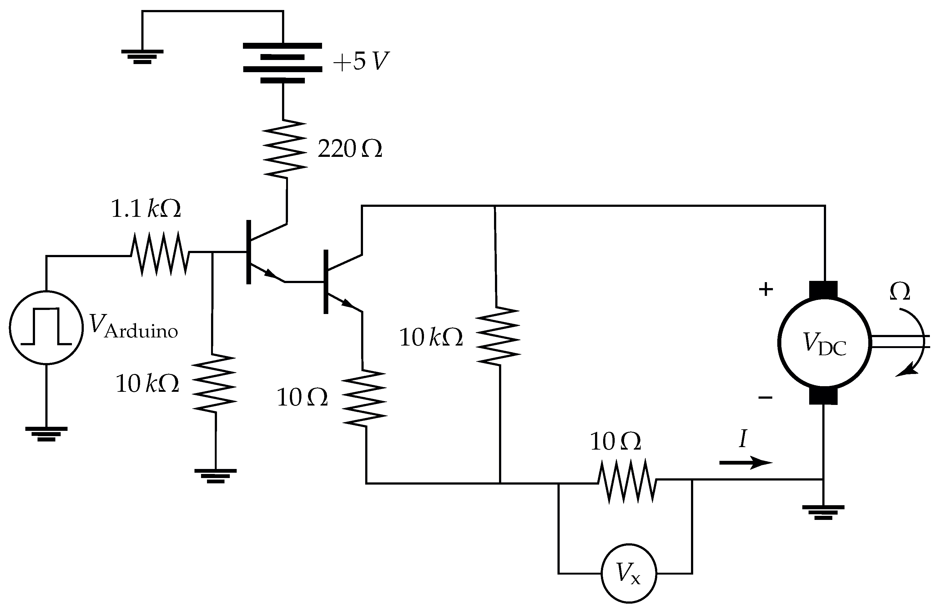
The wind turbine model used in this work was a three-bladed rotor with a diameter of . The Reynolds number based on the turbine diameter, the incoming velocity at hub height, and the kinematic viscosity was . The blades were designed following the recommendations of Bastankhah and Porté-Agel [29] for small-scale turbines, and their profiles were thus flat plates with a camber and thickness. The small differences between the rotor used in the current study and that described in [29], due to manufacturing constraints and the sharpness of the leading and trailing edges, resulted in a small change in the optimal blade pitch angle, as reported by Mazzeo et al. [30]. The rotor hub was coupled with a Faulhaber 2237S024CXR DC motor, here used as a generator. The operating point of the generator could be changed by varying the electrical load of the external circuit connected to its terminals. This was achieved digitally via an Arduino Mega to control the duty cycle of a transistor used as a switch, as depicted in Figure 3. When the transistor was on, a small resistor was connected in parallel to the large resistor in the main circuit. Increasing the on time of the transistor lowered the mean resistance observed by the generator, thus increasing the mean current I through the circuit and decreasing the angular velocity, , in analogy with one-quadrant chopper circuits used to control DC motors [31]. The mechanical torque Q that the turbine applied to the rotor shaft could be obtained indirectly by measuring the current I through the generator, according to the linear relation . Here, are constants obtained from the calibration of the generator [30]. The current I was in turn obtained indirectly by measuring the voltage drop across a known resistor (see Figure 3). The generator was equipped with a rotary encoder, enabling the determination of and therefore the computation of the mechanical power produced by the turbine, .
The turbine model was supported by an aluminium tower with a diameter of in the bottom half and in the top half, resulting in a hub height of . The tower was positioned downstream of the end of the roughness fetch, where the local boundary layer was no longer affected by the wakes of the roughness elements. Two CEA-06-125UNA-350 strain gauges were installed near the base of the tower, connected as two branches of a Wheatstone bridge in a half-bridge configuration and used to measure the thrust force T on the turbine. The strain gauges were calibrated daily by loading the tower with a set of known weights using a pulley. The tower was mounted on the shaft of a stepper motor, which was positioned inside the foam panels and thus isolated from the flow above to decrease its intrusivity. The stepper motor was controlled digitally with a second Arduino Mega, enabling the control of the yaw angle .
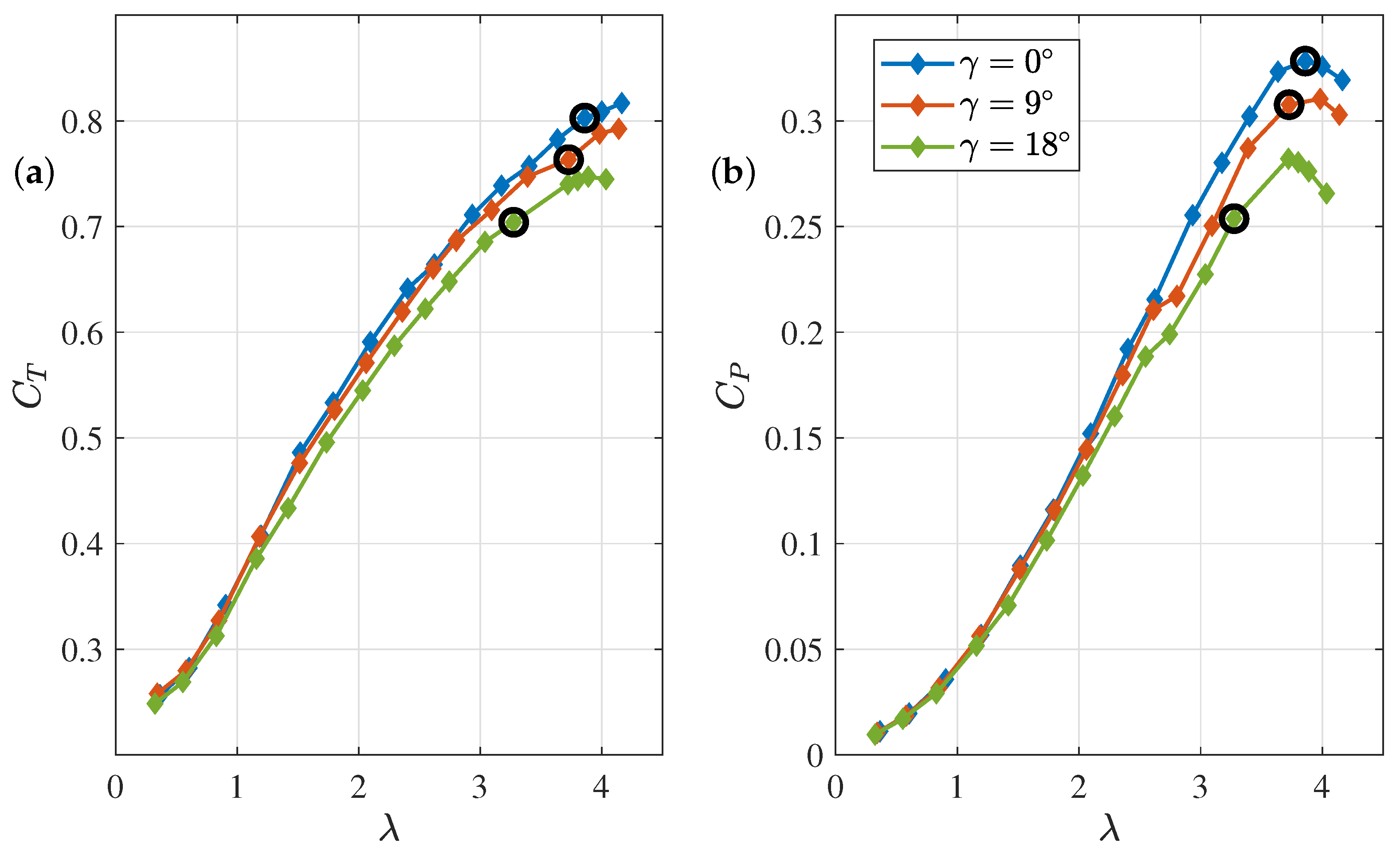
The thrust and power coefficient curves measured for = 0°, 9°, and 18° are shown in Figure 4. The maximum power coefficient when = 0° was and was found at the tip speed ratio . The respective thrust coefficient was . The black circles correspond to the turbine operating conditions achieved when the turbine was yawed but the generator set point was kept constant at the value that achieved when = 0°. Clearly, the turbine underwent a strong deceleration at high yaw angles.
The mechanical properties of the turbine (Q, T, and ), as well as the turbulent flow in its wake, were characterized by large fluctuations even when the yaw angle and the generator set point were kept constant. To remove this noise and to better identify the transient property variations that occurred when the yaw angle was changed, the analysis in this work was based on the ensemble averages of multiple time series measured by repeating the yawing maneuvers. These were obtained using a LabView program, which controlled both the data acquisition and the Arduino Mega connected to the stepper motor. With this program, the data sampling began at time , with the turbine set at the initial yaw angle . The rotation began at at a yawing rate of . This was a significantly higher than the rate typical of full-scale turbines (≈), but it was of the same order of magnitude as those used by Macrí et al. [21]. Once the maneuver was complete, the turbine was maintained at its current yaw angle for a time interval , at the end of which it was yawed back to . Data sampling continued until . A total of 75 velocity time series were saved at each measurement point, with , and . These values, however, were not sufficient to capture the completion of the transient and thus the attainment of a new steady state in the case of the turbine mechanical properties and Q, whose response to changes in the yaw angle was significantly slower. In these cases, the chosen parameters were and , and the ensemble average was obtained over 100 time series. The data acquisition of T, Q, and was carried out simultaneously with an NI cDAQ-9189, at a sampling frequency . The hot-wire signal was sampled at with an NI USB-6215. The uncertainty related to the starting time of the yawing maneuvers was approximately .
3. Results
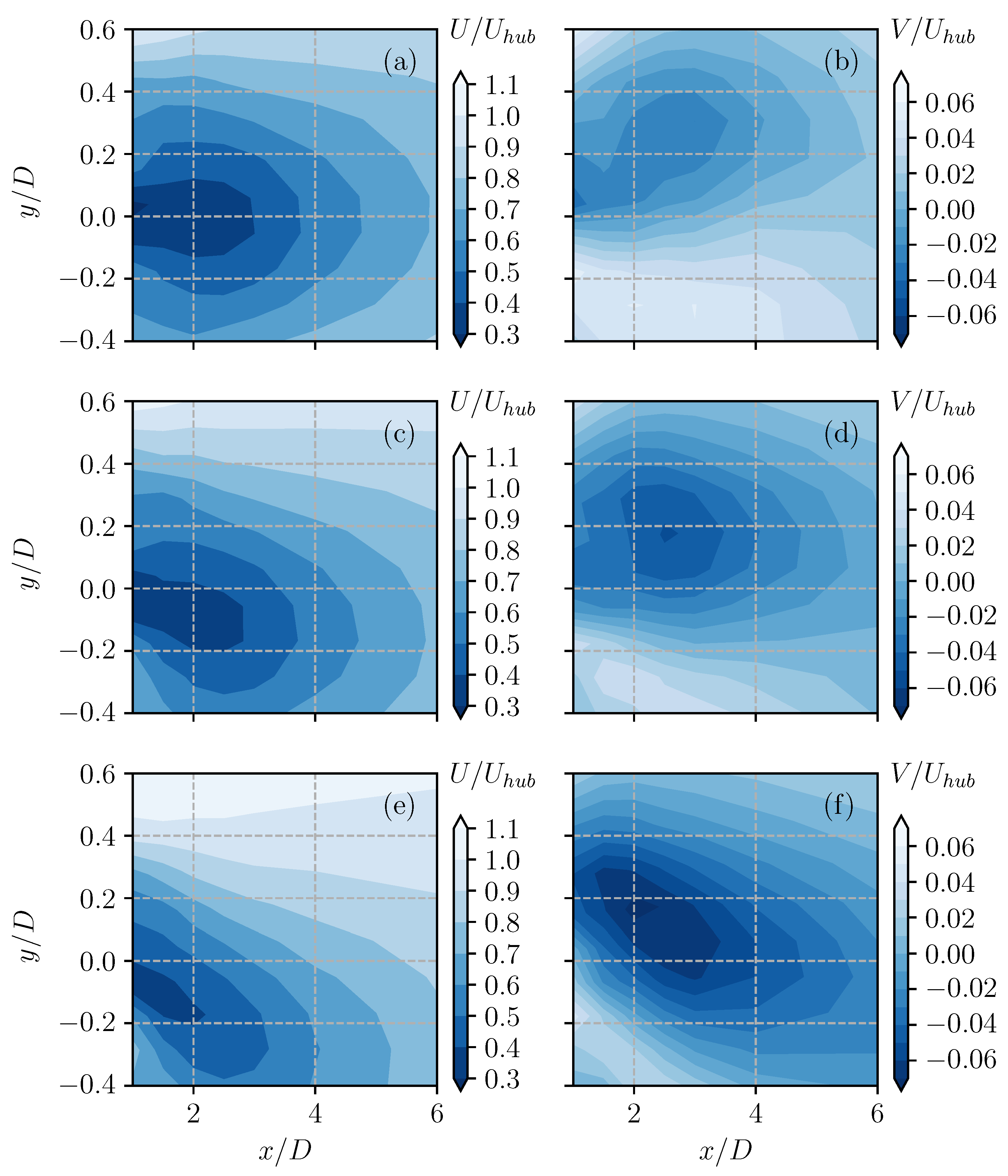
In order to provide context for the steady wake response, Figure 5 reports the stream-wise and radial velocity measured downwind of the wind turbine rotor at three different yaw angles (namely , , and ) to better visualize the wake deflection. As expected, the wake was symmetric around its axis in the non-yawed case, while it became increasingly skewed as the yaw angle increased. This is visible in both the stream-wise and radial velocity components, with the latter increasing significantly when the yaw angle was increased. A more detailed analysis of the steady-state wake of the turbine model used in this work was presented by Micheletto et al. [32].
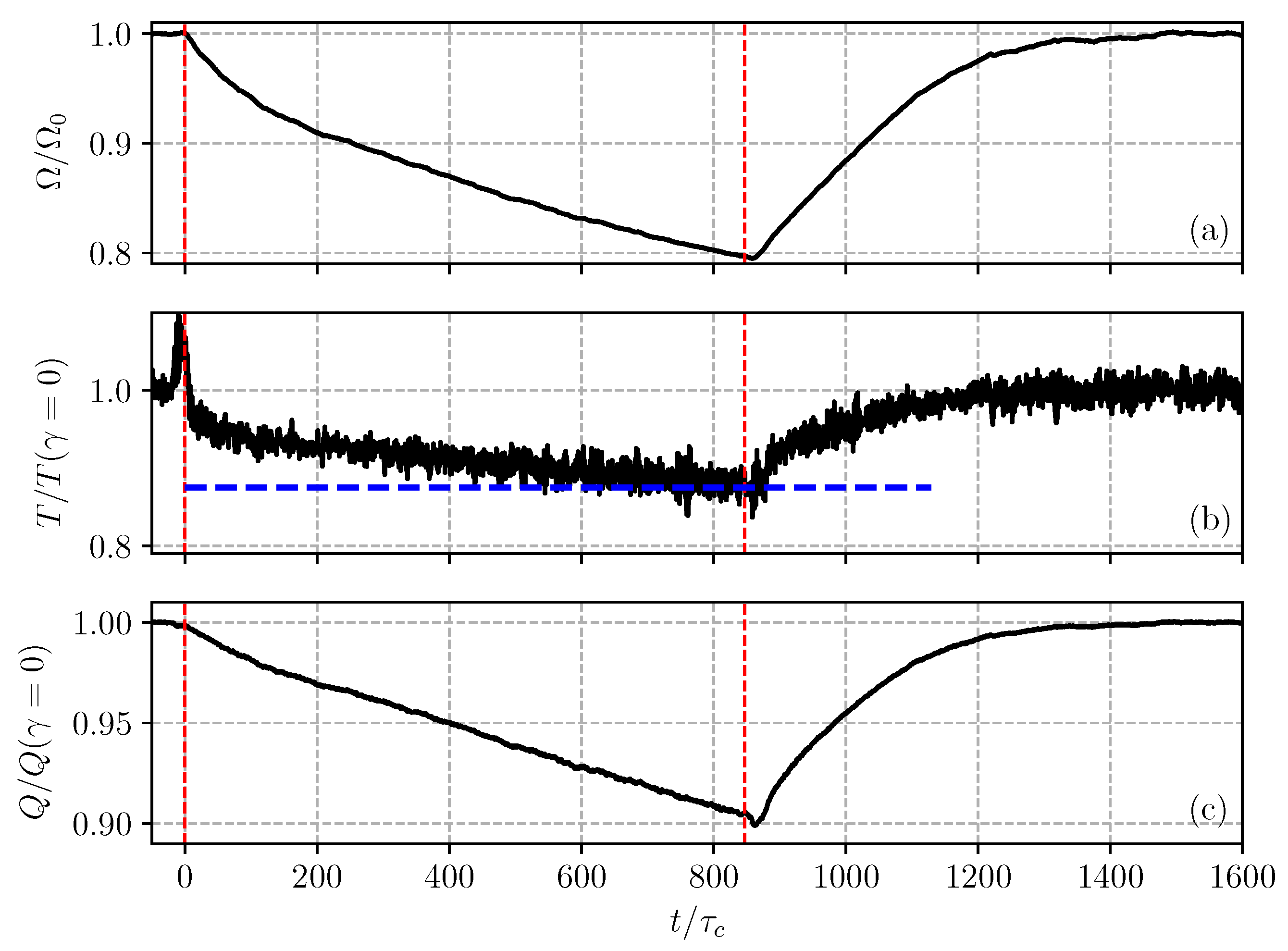
Figure 4 and Figure 5 represent the changes in the steady states at the turbine and in its wake that were reached well after the yaw angle had changed. The question of the temporal transition could be addressed by considering the time histories of the relevant quantities measured during the yaw actuation. Figure 6 reports the time series of the turbine scalar quantities, , T, and Q, during a yawing maneuver between and . It can be seen that both the angular velocity and the torque reacted slowly to the change in yaw angle, and neither quantity had converged even after 800 , where is a convective time scale. On the other hand, when the angle was decreased back to zero, the transient was much faster, and a relaxation time of only 400 was needed to achieve a converged value. The thrust seemed to follow a similar pattern, although its signal presented a spike at the first displacement (at the second displacement, it was barely visible). The same experiment performed with the transition between and did not indicate these behaviors, and all three quantities achieved a constant value within 400 from the beginning of the maneuver. On the other hand, the transition between and behaved similarly to Figure 6. The asymmetric behavior was mainly due to the fact that both the aerodynamic torque applied to the rotor and the generator breaking torque were nonlinear functions of . When the experiment with changing between and was repeated with a slightly reduced electrical load (higher breaking torque), the opposite behavior was observed: reached a new steady state only 400 after the first maneuver and more than 800 after the second one. This highlighted the importance of the motor set point in the dynamical response of a wind turbine.
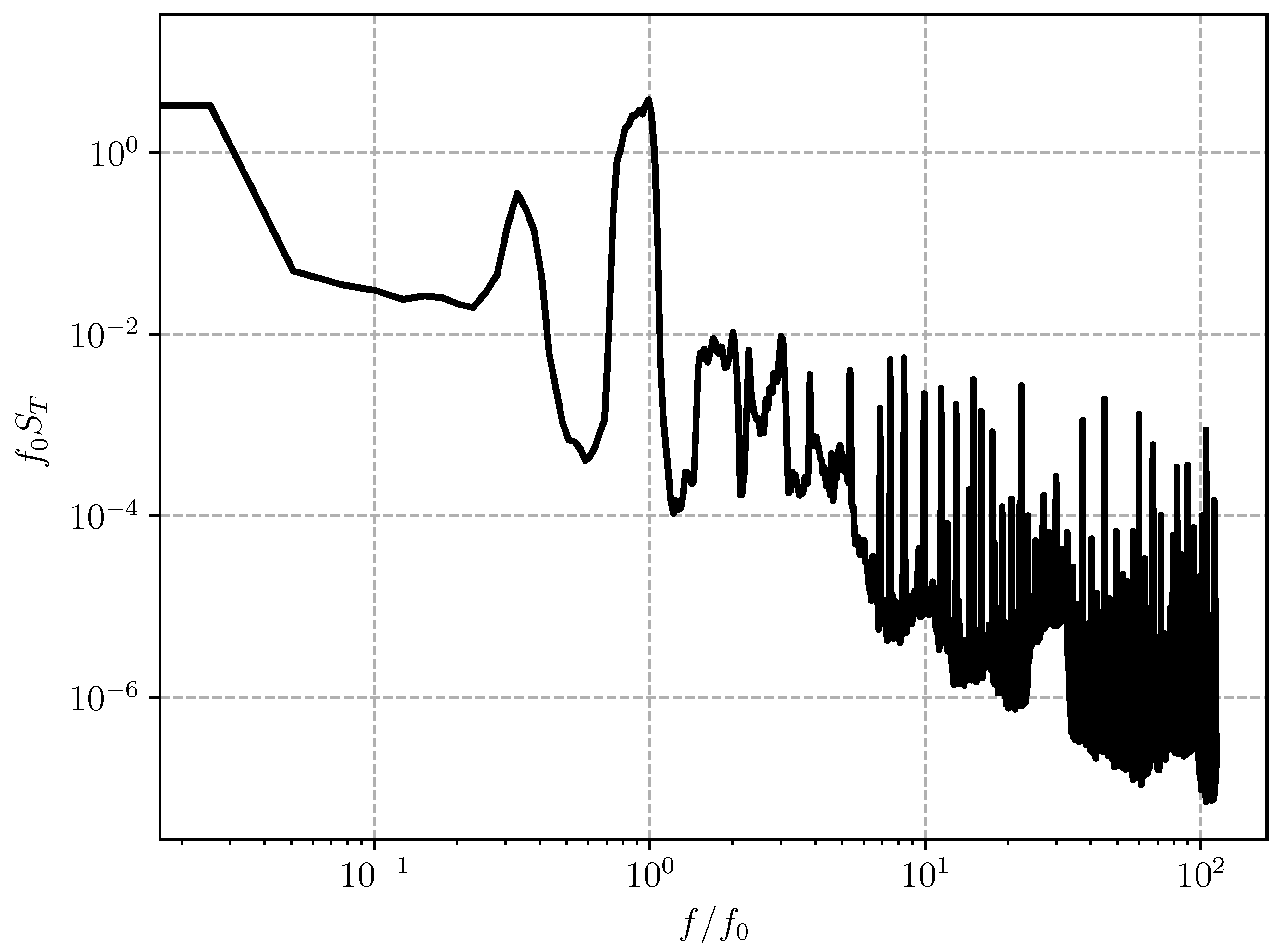
The thrust signal oscillated visibly, and in Figure 6 it was low-pass filtered by means of a moving average. When looking at its actual temporal evolution, it was possible to identify an oscillatory component due to the angular velocity of the turbine, in agreement with the findings of Mazzeo et al. [30]. This was also indicated by the power spectral density of the thrust signal, shown in Figure 7, where a peak around the turbine angular velocity, (with indicating the rotation frequency at a yaw angle of zero), was present. Due to the non-stationarity of the experiment, the power spectral density was polluted by the angle transitions, which result in a broadening of the peaks.
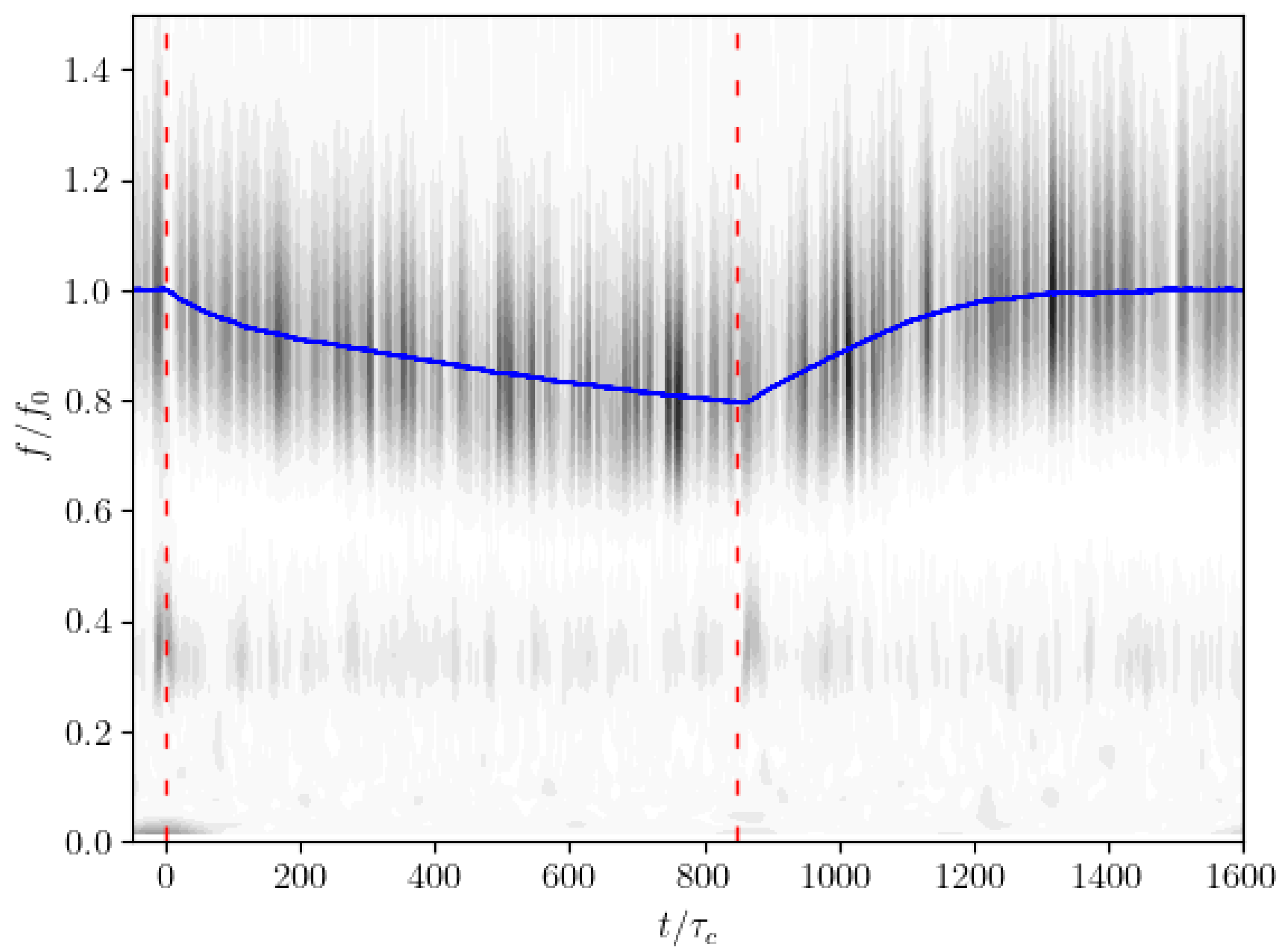
A more insightful approach required the examination of the time dependence of the frequencies contained in the signal. This was achieved by performing a wavelet analysis, using a Morlet wavelet, on the thrust force time series, as shown in Figure 8. Once again, a peak in the wavelet energy was visible around the instantaneous frequency of the wind turbine model. However, the wavelet transform indicated the emergence of a lower frequency that became dominant in the neighborhood of the yaw transition and weakened significantly within a few tenths of a second. This frequency shift was also clearly visible in the time history of the thrust force, and it was consistent for all the yaw maneuvers investigated in the present experiments. The torque and the angular velocity did not show similar oscillations.
While it was clear that the scalar quantities measured at the turbine required a long time to converge, it was important to also investigate the transition in the flow field downwind of the turbine, as this would affect the operation of other turbines placed in the wake. This was carried out by measuring the velocity in the wake of the turbine in the horizontal plane at hub height at nine spanwise positions () and seven streamwise positions (). First, 75 time series at each point were ensemble averaged. Then, the resulting time series were divided into three intervals: before the first yaw maneuver, between the first and the second maneuvers, and after the second maneuver. Time averaging was performed in each of the intervals, defining the corresponding steady states achieved after the transient regimes. The initial flow field was then subtracted from the entire time series, highlighting the deviation from the initial condition. At this point, the data were analyzed by means of the proper orthogonal decomposition (POD) technique.
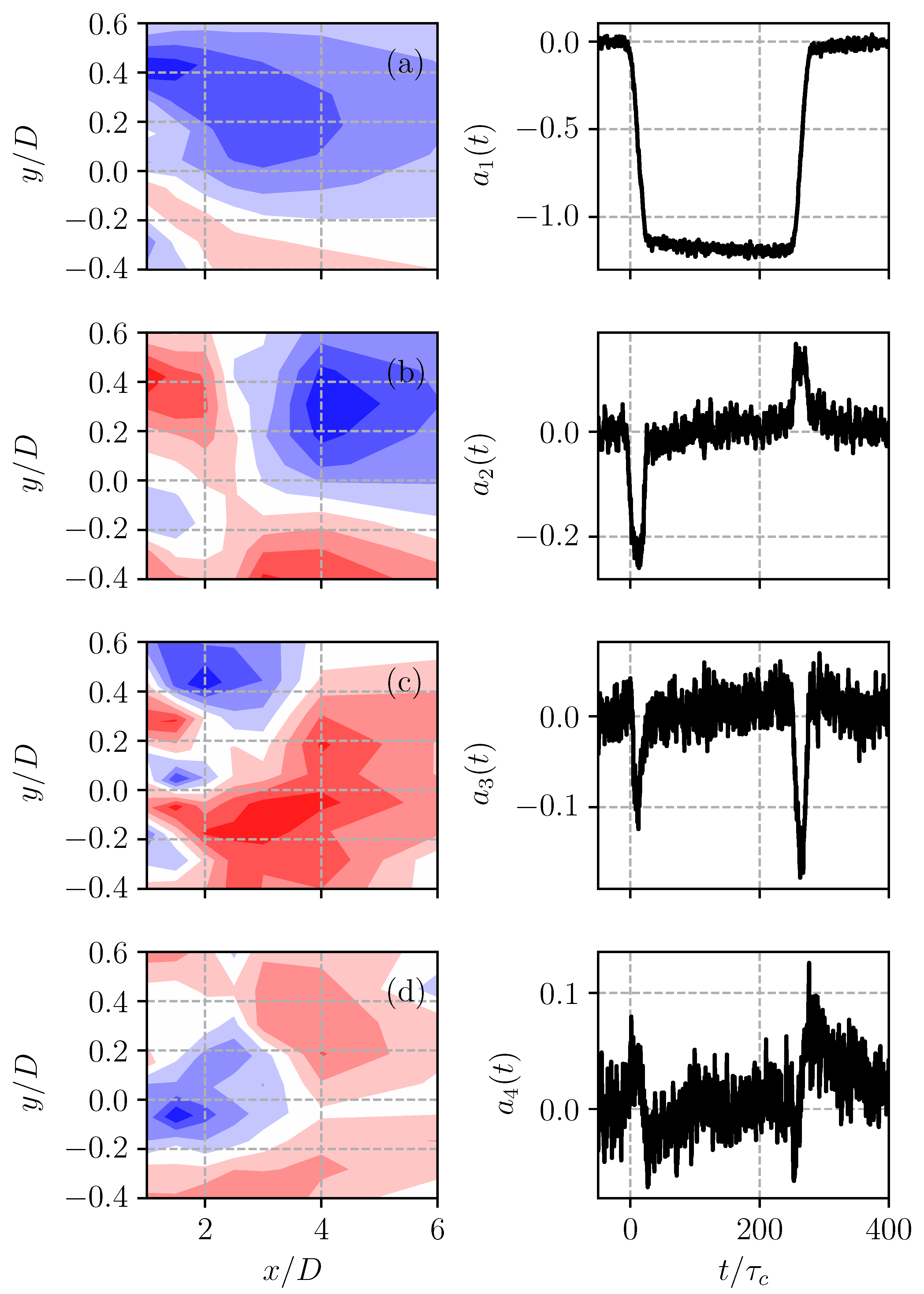
The first four leading modes, which accounted for the largest contributions to the variance in the transition between and , are presented in Figure 9, together with their respective temporal coefficients. The amplitude of the latter was clearly modulated by the yaw maneuvers. The first mode showed consistent behavior with the instantaneous yaw angle, and its spatial structure was given approximately by the difference in the steady states between the final angle and the initial angle.
The temporal coefficients of the second and third modes indicated that they were only active for around 20 , concurrently with the yaw transitions, and were otherwise inactive. Note that these were not paired modes associated with traveling waves. This was evinced by the fact that they presented different spatial structures. Furthermore, in the experiment with a yaw transition from to , even the active times of their temporal coefficients did not match. It could also be observed that the amplitude of the first mode coefficient was approximately one order of magnitude larger than that of the others, suggesting that a reduced-order model could be derived from the first mode alone. Such a simplification implied a uniform temporal adjustment throughout the spatial domain, while one would expect that the wake adjustment would propagate downwind as a transition front advected with the local velocity. Assuming that the front velocity was constant and given by the hub velocity [33], this front would traverse the monitored domain in just six convective time units. The yaw maneuver, in comparison, took 0.5 s or . The front propagation was therefore much faster than the maneuver. This suggested that, as a first approximation, the delay caused by the front-like propagation of the flow adjustment could be neglected. Furthermore, from the examination of the velocity time history at a single point, such as that in Figure 10 for a yaw change between and , it was clear that the transient in the flow field required a similar time to the maneuver (which is represented as a step-wise change in the figure but, as stated above, took approximately ). A similar observation was also noted in the experiment with changing between and . The aerodynamics could therefore be considered quasi-stationary with the wake adjusting instantaneously to the current yaw angle.
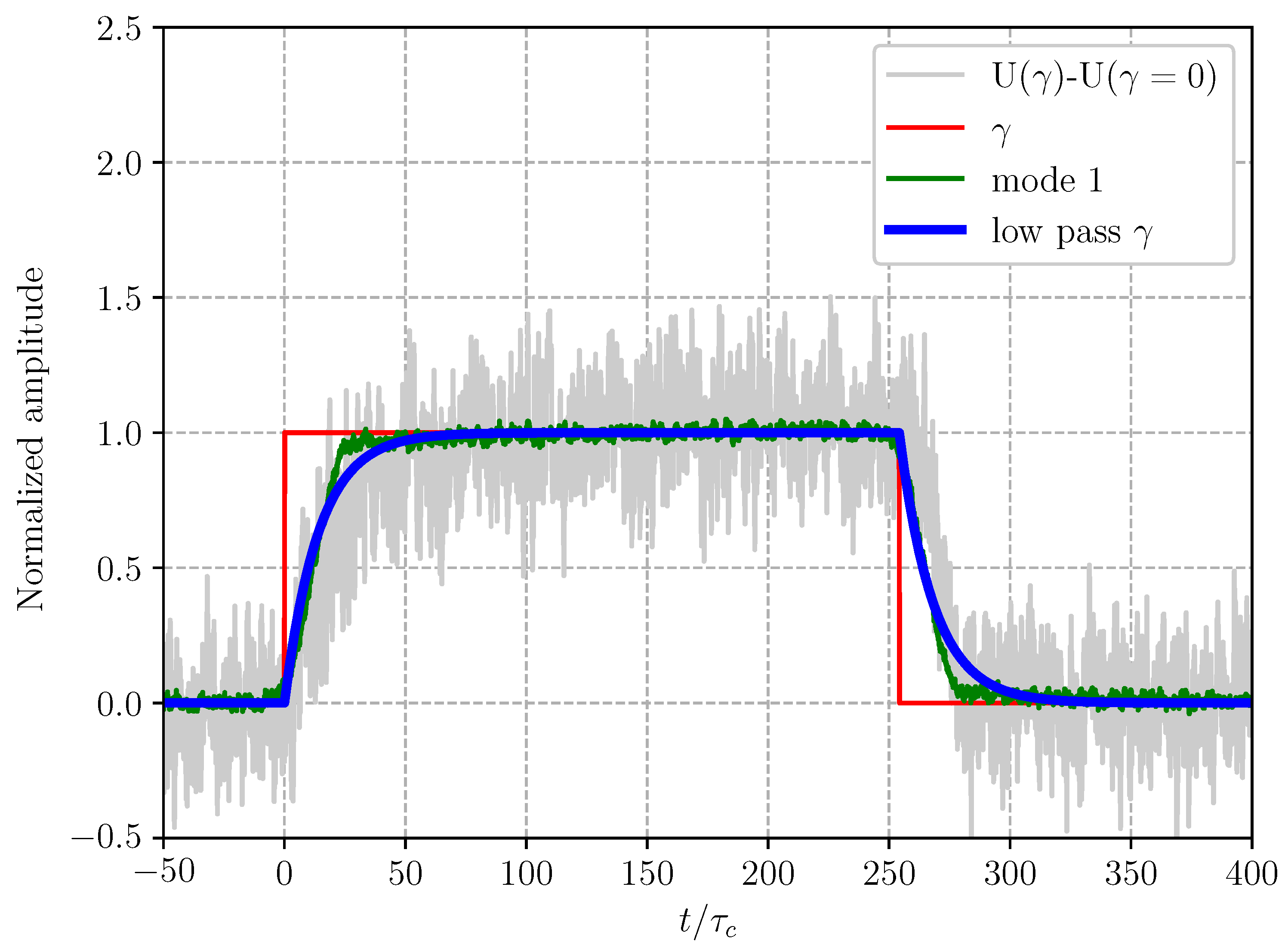
Figure 10 also shows that the temporal coefficient of the first POD mode (that filtered out small-scale noise) followed well the noisier velocity signal measured at a point in the wake and presented sharp corners at both the beginning and end of the yawing maneuver, associated with the ramp change in the instantaneous yaw angle. This agreement supported the hypothesis that a reduced-order model based on the first POD mode could adequately describe the flow field transient. Finally, the figure also includes the approximation of the temporal coefficient of the first POD mode, , as a first-order filter in the form
where is the characteristic time scale of the filter. Once again, this temporal constant was closely related to the actuation time and the flow inertia, although the latter was much shorter than the former. The agreement between the POD coefficient and the modeled value obtained from Equation (1) was reasonably good, although the latter failed to capture the sharp changes in the temporal coefficient taking place at the end of the two transients.
4. A Simple Model for Wind Farm Transients
As a result of the POD analysis of the previous section, it is here proposed that the transition between the initial state, , and a final state, , can be approximated by means of the parametric relationship
where quantifies the state difference during the transient, which is 0 before the transition and 1 when the transition is completed. The analysis of the time series of the velocity field, as well as of the first POD mode coefficient, pointed out that the leading temporal adjustment could be sufficiently described using a first-order model given by
While Equation (2) is natural for the simple transition cases discussed in the present work, it is complicated to apply when multiple transitions take place (for example, in the cases of consecutive changes in wind direction or simultaneous yawing maneuvers by multiple turbines). Therefore, it was worth investigating alternative formulations of Equation (2) that exploit the instantaneous state rather than an initial state. In this respect, one could write Equation (2) at the next time instant as
and, by taking the difference between (4) and (2), one could obtain
The coefficient in front of the square brackets is the temporal adjustment coefficient that relates the shift from the present status, , to the final one, . The latter can also be time-dependent, and it is only related to the desired final set point. By considering an infinitesimal time step, , it is possible to exploit Equation (3), so that (6) becomes
which is the desired expression. The main advantage of Equation (7) compared to the initial Expression (2) is that the initial state is not required, and the evolution of the flow field after a variety of transitions can be taken into account. On the other hand, while Equation (3) can be solved analytically with a simple yaw transition, and the flow field can be computed at any arbitrary time, Equation (7) must be integrated numerically by time-step marching. Numerical stability requirements impose that , a constraint that can be circumvented using the implicit version of (7). This is obtained by deriving the expression for from (2) evaluated at time and then exploiting Equation (3). In this way, Equation (6) becomes
The time constant, , is determined by a combination of the flow response and the inertia of the turbine and the actuators. In this experiment, the constant was comparable with the maneuver time of the turbine, a condition that is expected to be realistic even in large-scale wind turbines.
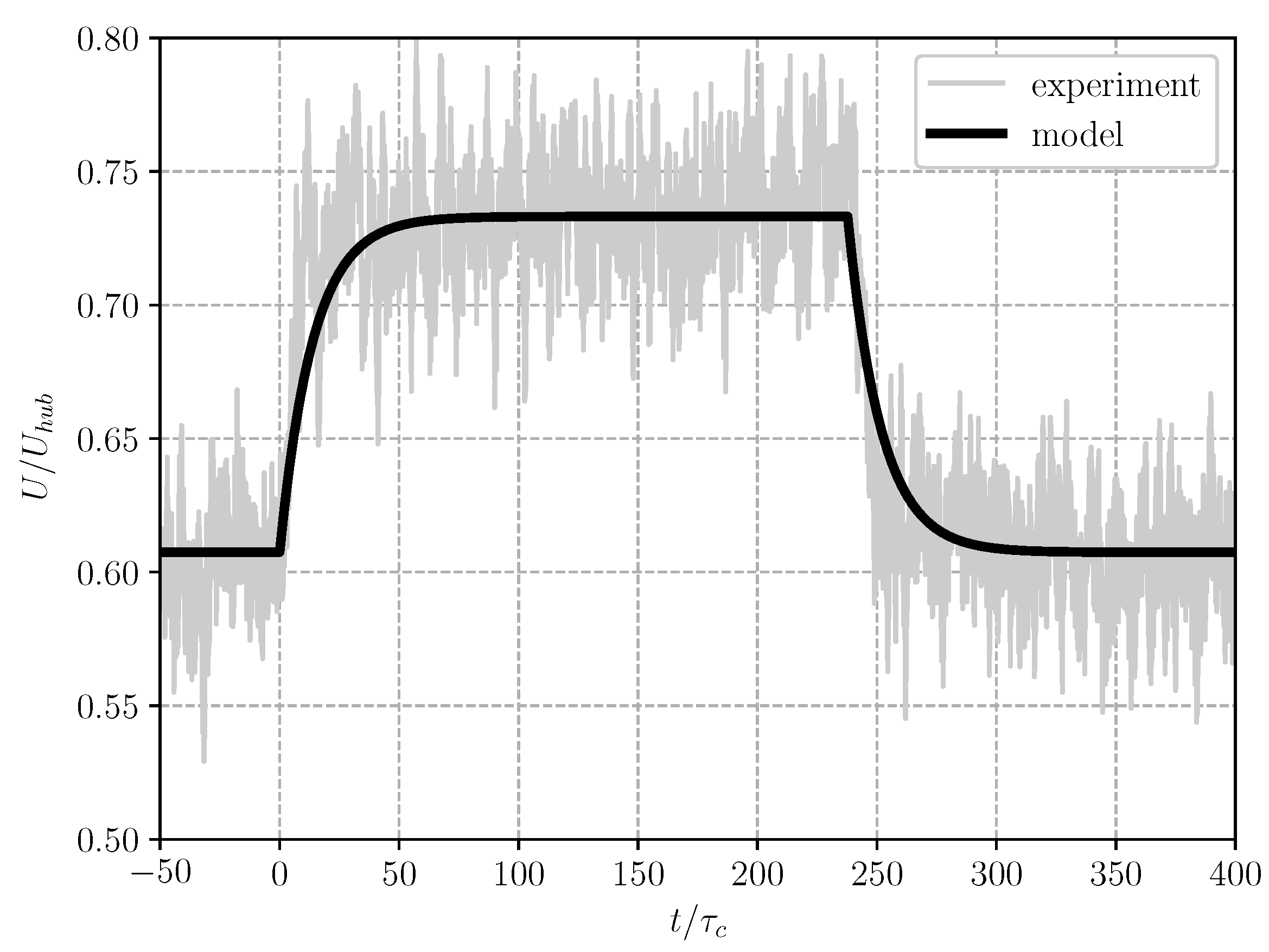
To demonstrate the validity of the model, Figure 11 displays a comparison between the model prediction and the measured velocity time series at one point in the monitored domain for the transition between and . The final states used in Equation (8) for each of the two maneuvers are given by the steady states at or (the latter being chosen if the time was according to the maneuver times in the experiment). As seen in the figure, the agreement between the data and the model was reasonably good. Once again, the value of this model lies in its mapping of the velocity transient that follows a yaw transition. The final states were obtained from the present experimental data, but they could also be computed from steady wake models.
5. Discussion and Final Remarks
The characterization of wind turbine wake transients is an important building block for control schemes wherein both the inflow and operating conditions change over time. Experiments with a windt urbine model performing several yaw maneuvers were analyzed in order to characterize how the scalar parameters and wake velocity adjusted to the new set point. Scalar quantities measured at the rotor are directly associated with fatigue loads and turbine performance. From the present results, it was evident that Q, T, and shared similar adjustment times, and this was not surprising, as the three quantities are not independent. The characteristic time scale to achieve a steady state was one order of magnitude larger than the duration of the yawing maneuver, suggesting that the dynamics of the turbine scalar quantities were governed by the inertia of the rotor and the generator. Interestingly, for all the available yaw maneuvers, q it was observed that the energy spectrum of the thrust signal had a distinct peak at the instantaneous angular frequency of the rotor, while a lower frequency peak appeared only during the rapid yaw transition and disappeared soon afterwards.
The experiments also showed that the flow relaxation time was very close to the yawing maneuver duration, in agreement with the findings of Macrì et al. [21] for a porous disk. The POD analysis of the flow field in the wake highlighted that the velocity transients were well characterized by means of a few modes. The most energetic one was associated with the global flow field modification in the steady states, while higher-order modes were related to faster transients. In order to develop a feasible reduced-order model, only the first mode was taken into account, and the temporal coefficient was modeled by means of a first-order low-pass filter. Consequently, one of the main assumptions of the reduced-order model was that the velocity transient began simultaneously across the whole domain, while the front-like propagation of the flow adjustment was neglected. This was justified in the present work by the fact that, for laboratory-scale turbines, the convective time scale is very small (), and the time required for the front to travel across the domain is much shorter than the yaw actuation time. In the case of a full-scale wind farm, however, would be of the order of 10 s, and the time for a wave front to cross the spacing between turbines could be similar to or larger than the actuation time. This would result in a non-negligible delay time for the start of the transient in the far wake, which the model presented in this work would fail to capture. A simple improvement could be made by adopting a locally adjusted time variable , where is an advection delay function. It should be noted that Macrì et al. [21] found that the actual delay is usually longer than that predicted using , most notably when the turbine is realigned with the flow. A more complete understanding of the spatial dependence of the adjustment propagation would require time-resolved spatial data. The hot-wire measurements performed in the present work only provided time-resolved data at a single point. The spatial information was recovered by performing multiple measurements triggered by the yaw maneuvers. It is possible that performing an ensemble average on multiple time series at each point, in combination with incoming high- and low-velocity structures from the turbulent ABL and the fact that the adjustment front traveled with the local velocity rather than with a fixed reference speed, resulted in the masking of any front-like behavior. This would explain why the POD analysis did not reveal a pair of modes representing traveling waves. In any case, it is likely that in the presence of a turbulent inflow, the front-like propagation would be damped. It is important to stress that even if such a delay was neglected, the transient behavior predicted by this model would be correct and simply shifted along the time axis, because the time constant only depends on the turbine inertia and the actuation time. The extension of this transient model to a wind farm where multiple turbines can change their yaw angle was made trivial by means of Equation (8), which should be regarded as the method of choice. It is worth mentioning that no partial differential equation was solved here, but rather the approach provided the temporal evolution at each observed point, similarly to the output of the POD analysis, with a simple time-marching algorithm. The main advantage of this method was that the analysis only needed two flow conditions, namely the actual state and the final steady state, which can be computed from wake models or intensive numerical simulations of a wind farm.
Author Contributions
Conceptualization, D.M., A.S. and J.H.M.F.; methodology, D.M., A.S. and J.H.M.F.; software, D.M. and A.S.; validation, D.M. and A.S.; formal analysis, D.M. and A.S.; investigation, D.M.; resources, D.M.; data curation, D.M. and A.S.; writing—original draft preparation, D.M. and A.S.; writing—review and editing, D.M., A.S. and J.H.M.F.; visualization, A.S. and D.M.; supervision, A.S. and J.H.M.F.; project administration, J.H.M.F.; funding acquisition, A.S. All authors have read and agreed to the published version of the manuscript.
Funding
This research was funded by the Swedish Energy with grant number 48649-1.
Data Availability Statement
Data are available upon request.
Acknowledgments
Aldo Romani is acknowledged for his useful suggestions regarding the development of the hardware for controlling the turbine angular velocity. STandUP for Wind is also acknowledged.
Conflicts of Interest
The authors declare no conflict of interest.
References
- REN21. Renewables 2023 Global Status Report Collection, Renewables in Energy Supply; REN21 Secretariat: Paris, France, 2023; ISBN 978-3-948393-08-3. [Google Scholar]
- Shapiro, C.R.; Starke, G.M.; Gayme, D.F. Turbulence and Control of Wind Farms. Annu. Rev. Control Robot. Auton. 2022, 5, 579–602. [Google Scholar] [CrossRef]
- Ekelund, T. Yaw control for reduction of structural dynamic loads in wind turbines. J. Wind Eng. Ind. Aerodyn. 2000, 85, 241–262. [Google Scholar] [CrossRef]
- Barlas, T.; van Kuik, G. Review of state of the art in smart rotor control research for wind turbines. Prog. Aero. Sci. USA 2010, 46, 1–27. [Google Scholar] [CrossRef]
- Howland, M.F.; Lele, S.K.; Dabiri, J.O. Wind farm power optimization through wake steering. Proc. Natl. Acad. Sci. USA 2019, 116, 14495–14500. [Google Scholar] [CrossRef] [PubMed] [Green Version]
- Munters, W.; Meyers, J. Dynamic Strategies for Yaw and Induction Control of Wind Farms Based on Large-Eddy Simulation and Optimization. Energies 2018, 11, 177. [Google Scholar] [CrossRef] [Green Version]
- Chamorro, L.P.; Lee, S.J.; Olsen, D.; Milliren, C.; Marr, J.; Arndt, R.; Sotiropoulos, F. Tuebulence effectes on a full-scale 2.5 MW horizontal-axis wind turbine under neutrally stratified conditions. Wind Energy 2015, 18, 339–349. [Google Scholar] [CrossRef]
- Antonutti, R.; Peyrard, C.; Johanning, L.; Incecik, A.; Ingram, D. The effects of wind-induced inclination on the dynamics of semi-submersible floating wind turbines in the time domain. Renew. Energy 2016, 88, 83–94. [Google Scholar] [CrossRef] [Green Version]
- Tobin, N.; Zhu, H.; Chamorro, L.P. Spectral behaviour of the turbulence-driven power fluctuations of wind turbines. J. Turbul. 2015, 16, 832–846. [Google Scholar] [CrossRef]
- Zhang, B.; Jin, Y.; Cheng, S.; Zheng, Y.; Chamorro, L.P. On the dynamics of a model wind turbine under passive tower oscillations. Appl. Energy 2022, 311, 118608. [Google Scholar] [CrossRef]
- Bastankhah, M.; Porté-Agel, F. Experimental and theoretical study of wind turbine wakes in yawed conditions. J. Fluid Mech. 2016, 806, 506–541. [Google Scholar] [CrossRef]
- Shapiro, C.R.; Gayme, D.F.; Meneveau, C. Modelling yawed wind turbine wakes: A lifting line approach. J. Fluid Mech. 2018, 841, R1. [Google Scholar] [CrossRef] [Green Version]
- Gebraad, P.M.O.; van Wingerden, J.W. A Control-Oriented Dynamic Model for Wakes in Wind Plants. J. Phys. Conf. Ser. 2014, 524, 012186. [Google Scholar] [CrossRef]
- Becker, M.; Allaerts, D.; van Wingerden, J.W. FLORIDyn—A dynamic and flexible framework for real-time wind farm control. J. Phys. Conf. Ser. 2022, 2265, 032103. [Google Scholar] [CrossRef]
- Foloppe, B.; Munters, W.; Buckingham, S.; Vandevelde, L.; van Beeck, J. Development of a dynamic wake model accounting for wake advection delays and mesoscale wind transients. J. Phys. Conf. Ser. 2022, 2265, 022055. [Google Scholar] [CrossRef]
- Gebraad, P.M.O.; Teeuwisse, F.W.; van Wingerden, J.W.; Fleming, P.A.; Ruben, S.D.; Marden, J.R.; Pao, L.Y. Wind plant power optimization through yaw control using a parametric model for wake effects—A CFD simulation study. Wind Energy 2016, 19, 95–114. [Google Scholar] [CrossRef]
- Lejeune, M.; Moens, M.; Chatelain, P. A Meandering-Capturing Wake Model Coupled to Rotor-Based Flow-Sensing for Operational Wind Farm Flow Prediction. Front. Energy Res. 2022, 10, 884068. [Google Scholar] [CrossRef]
- Ebrahimi, A.; Sekandari, M. Transient response of the flexible blade of horizontal-axis wind turbines in wind gusts and rapid yaw changes. Energy 2018, 145, 261–275. [Google Scholar] [CrossRef]
- Abraham, A.; Martínez-Tossas, L.A.; Hong, J. Mechanisms of dynamic near-wake modulation of a utility-scale wind turbine. J. Fluid Mech. 2021, 926, A29. [Google Scholar] [CrossRef]
- Yu, W.; Hong, V.; Ferreira, C.; Kuik, G. Experimental analysis on the dynamic wake of an actuator disc undergoing transient loads. Exp. Fluids 2017, 58, 149. [Google Scholar] [CrossRef] [Green Version]
- Macrí, S.; Aubrun, S.; Leroy, A.; Girard, N. Experimental investigation of wind turbine wake and load dynamics during yaw maneuvers. Wind Energ. Sci. 2021, 6, 585–599. [Google Scholar] [CrossRef]
- Abraham, A.; Hong, J. Dynamic wake modulation induced by utility-scale wind turbine operation. Appl. Energy 2020, 257, 114003. [Google Scholar] [CrossRef]
- Lindgren, B.; Johansson, A.V. Evaluation of the Flow Quality in the MTL Wind-Tunnel; Report TRITA-MEK; Department of Mechanics, KTH: Stockholm, Sweden, 2002. [Google Scholar]
- Counihan, J. An improved method of simulating an atmospheric boundary layer in a wind tunnel. Atmos. Environ. 1969, 3, 197–214. [Google Scholar] [CrossRef]
- Hohman, T.C.; Van Buren, T.; Martinelli, L.; Smits, A. Generating an artificially thickened boundary layer to simulate the neutral atmospheric boundary layer. J. Wind Eng. Ind. Aerodyn. 2015, 145, 1–16. [Google Scholar] [CrossRef]
- Bottema, M. Urban roughness modelling in relation to pollutant dispersion. Atmos. Environ. 1997, 31, 3059–3075. [Google Scholar] [CrossRef]
- Örlü, R.; Fransson, J.H.; Henrik Alfredsson, P. On near wall measurements of wall bounded flows—The necessity of an accurate determination of the wall position. Prog. Aerosp. Sci. 2010, 46, 353–387. [Google Scholar] [CrossRef]
- Counihan, J. Adiabatic atmospheric boundary layers: A review and analysis of data from the period 1880–1972. Atmos. Environ. 1975, 9, 871–905. [Google Scholar] [CrossRef]
- Bastankhah, M.; Porté-Agel, F. A new miniature wind turbine for wind tunnel experiments. Part I: Design and performance. Energies 2017, 10, 908. [Google Scholar] [CrossRef] [Green Version]
- Mazzeo, F.; Micheletto, D.; Talamelli, A.; Segalini, A. An Experimental Study on a Wind Turbine Rotor Affected by Pitch Imbalance. Energies 2022, 15, 8665. [Google Scholar] [CrossRef]
- Rizzoni, G. Fundamentals of Electrical Engineering; McGraw-Hill Education: New York, NY, USA, 2008. [Google Scholar]
- Micheletto, D.; Segalini, A.; Fransson, J.H.M. Experimental analysis of the wake behind a small wind-turbine model in yaw. J. Phys. Conf. Ser. 2023, 2505, 012030. [Google Scholar] [CrossRef]
- Trujillo, J.J.; Bingöl, F.; Larsen, G.C.; Mann, J.; Kühn, M. Light detection and ranging measurements of wake dynamics. Part II: Two-dimensional scanning. Wind Energy 2011, 14, 61–75. [Google Scholar] [CrossRef]
Figure 1.
Schematic representation of the experimental setup seen from the side, not to scale. Moving from left to right, the uniform flow encounters the castellated barrier, then the spires, and finally the distributed roughness. Note the presence of the foam panels acting as the effective floor, inside of which the stepper motor is represented with dashed lines. All dimensions are in millimeters.

Figure 2.
Profiles of the mean (a) and standard deviation (b) of the stream-wise velocity, normalized with the undisturbed hub velocity and hub height . The measurements were performed downstream of the end of the roughness fetch. The dashed lines indicate hub height, and the dashed-dotted lines delimit the region swept by the rotor. (c) Mean streamwise velocity profile in semilogarithmic scale. The red line represents the fitted logarithmic law, and the dashed-dotted lines indicate the fitting bounds.

Figure 3.
Electrical circuit connected to the generator used to control the angular velocity and monitor the current I.
Figure 3.
Electrical circuit connected to the generator used to control the angular velocity and monitor the current I.

Figure 4.
(a) Thrust and (b) power coefficients at different values for three yaw angles. The black circles represent the steady-state conditions obtained before and after the yawing maneuvers while keeping the set point of the generator the same.
Figure 4.
(a) Thrust and (b) power coefficients at different values for three yaw angles. The black circles represent the steady-state conditions obtained before and after the yawing maneuvers while keeping the set point of the generator the same.

Figure 5.
Time-averaged stream-wise (left) and radial (right) velocity field at (a,b); (c,d); and (e,f).
Figure 5.
Time-averaged stream-wise (left) and radial (right) velocity field at (a,b); (c,d); and (e,f).

Figure 6.
Temporal evolution of the turbine angular velocity (a), thrust T (b), and torque Q (c) during a step increase in the yaw angle from to . The red dashed lines indicate the temporal interval where the yaw angle was . The blue dashed line in (b) indicates the value of from the curve shown in Figure 4. The quantities were normalized with their value when the yaw was . To eliminate rapid fluctuations, a moving average with a 33 ms time window was applied to all time series.

Figure 7.
Power spectral density of the thrust signal for the experiment with the transition from to . Frequencies were normalized with the turbine rotation frequency.
Figure 7.
Power spectral density of the thrust signal for the experiment with the transition from to . Frequencies were normalized with the turbine rotation frequency.

Figure 8.
Squared norm of the wavelet transform of the thrust signal for the experiment with the transition from to (the instants of the transitions are marked by red vertical lines). The blue line indicates the instantaneous angular frequency of the turbine.
Figure 8.
Squared norm of the wavelet transform of the thrust signal for the experiment with the transition from to (the instants of the transitions are marked by red vertical lines). The blue line indicates the instantaneous angular frequency of the turbine.

Figure 9.
First four POD modes of the experiment with yaw transition between and . The left column shows the spatial modes ((a–d), denoting the first to fourth modes, respectively), while the right column contains the associated temporal coefficients of the modes.
Figure 9.
First four POD modes of the experiment with yaw transition between and . The left column shows the spatial modes ((a–d), denoting the first to fourth modes, respectively), while the right column contains the associated temporal coefficients of the modes.

Figure 10.
Ensemble average of the axial velocity at and over a transition from to (gray line) in response to the yaw angle of the turbine (red line). The first mode temporal coefficient is also plotted (green line), together with a first-order filter (blue line). The time series were normalized by subtracting the initial value and dividing by the regime value at .

Figure 11.
Ensemble average of the axial velocity at and over a transition from to and back (gray line). The black line is the estimated velocity field from the proposed model.
Figure 11.
Ensemble average of the axial velocity at and over a transition from to and back (gray line). The black line is the estimated velocity field from the proposed model.

Disclaimer/Publisher’s Note: The statements, opinions and data contained in all publications are solely those of the individual author(s) and contributor(s) and not of MDPI and/or the editor(s). MDPI and/or the editor(s) disclaim responsibility for any injury to people or property resulting from any ideas, methods, instructions or products referred to in the content. |
© 2023 by the authors. Licensee MDPI, Basel, Switzerland. This article is an open access article distributed under the terms and conditions of the Creative Commons Attribution (CC BY) license (https://creativecommons.org/licenses/by/4.0/).
Share and Cite
MDPI and ACS Style
Micheletto, D.; Fransson, J.H.M.; Segalini, A. Experimental Study of the Transient Behavior of a Wind Turbine Wake Following Yaw Actuation. Energies 2023, 16, 5147. https://doi.org/10.3390/en16135147
AMA Style
Micheletto D, Fransson JHM, Segalini A. Experimental Study of the Transient Behavior of a Wind Turbine Wake Following Yaw Actuation. Energies. 2023; 16(13):5147. https://doi.org/10.3390/en16135147
Chicago/Turabian StyleMicheletto, Derek, Jens H. M. Fransson, and Antonio Segalini. 2023. "Experimental Study of the Transient Behavior of a Wind Turbine Wake Following Yaw Actuation" Energies 16, no. 13: 5147. https://doi.org/10.3390/en16135147
Note that from the first issue of 2016, this journal uses article numbers instead of page numbers. See further details here.