
Study on the Effect of Structural Parameters of Volume Control Tank on Gas–Liquid Mass Transfer


1
State Key Laboratory of Nuclear Power Safety Technology and Equipment, China Nuclear Power Engineering Co., Ltd., Shenzhen 518172, China
2
Institute of Thermal Science and Technology, Shandong University, Jinan 250061, China
*
Author to whom correspondence should be addressed.
Energies 2023, 16(13), 4991; https://doi.org/10.3390/en16134991
Submission received: 18 May 2023
/
Revised: 14 June 2023
/
Accepted: 21 June 2023
/
Published: 27 June 2023
Abstract
:The volume control tank (VCT) is an important facility in the primary circuit of nuclear power plants. During the normal operation of nuclear power plants, the mass transfer between the gas and liquid phases occurs in the VCT at all times. It is driven by submerged jets, which may cause potential risks to the operational safety of nuclear power plants. It is necessary to conduct an in-depth study to gain a deeper understanding of the gas–liquid mass transfer behavior in the VCT. In this paper, a new gas–liquid mass transfer model is developed that combines a surface divergence model with a CFD model to accurately simulate the mass transfer process of the gas phase into the liquid phase. The simulation data were verified by the experimental results. The deviation between the simulation results and experimental results is less than 6.55%. Based on this model, a simulation study was carried out for the effect of structural parameters of the VCT on gas–liquid mass transfer. The results show that the double-vortex structure above the jet inlet, the surface jet at the gas–liquid interface, and the vortex at the end of the jet are the three factors dominating the gas–liquid mass transfer in the VCT. The gas–liquid mass transfer can be influenced by the jet diameter since the jet diameter has a remarkable effect on the Kolmogorov scale and the macroscopic flow field structure. Moreover, both the Kolmogorov scale and the macroscopic flow field structure can be affected by the jet height. However, these two effects cancel each other out. Thus, the influence of the jet height on the gas–liquid mass transfer rate is negligible.
1. Introduction
With the progression of time, global pollution issues and energy depletion are gradually being paid attention to. The transition from fossil energy to renewable and clean energy is an inevitable development for humanity. Renewable energy sources, such as wind, solar, and hydro, are constrained by climate and geography. In contrast, nuclear power, as a zero-carbon and high-efficiency power generation method, is an essential means of achieving carbon peaking and carbon neutrality. In recent years, the proportion of nuclear power generation to total electricity generation has been increasing internationally, and the safety of nuclear power has become a matter of public concern. Since the first use of nuclear power to generate electricity in the United States in 1951, there have been three major nuclear power accidents, the most recent occurring in 2011 at the Fukushima Daiichi nuclear power plant. In addition, there have been a number of minor safety incidents, and the safety of nuclear power is a growing concern. The discharge and disposal of radioactive waste from nuclear power plants have also been a significant public concern.
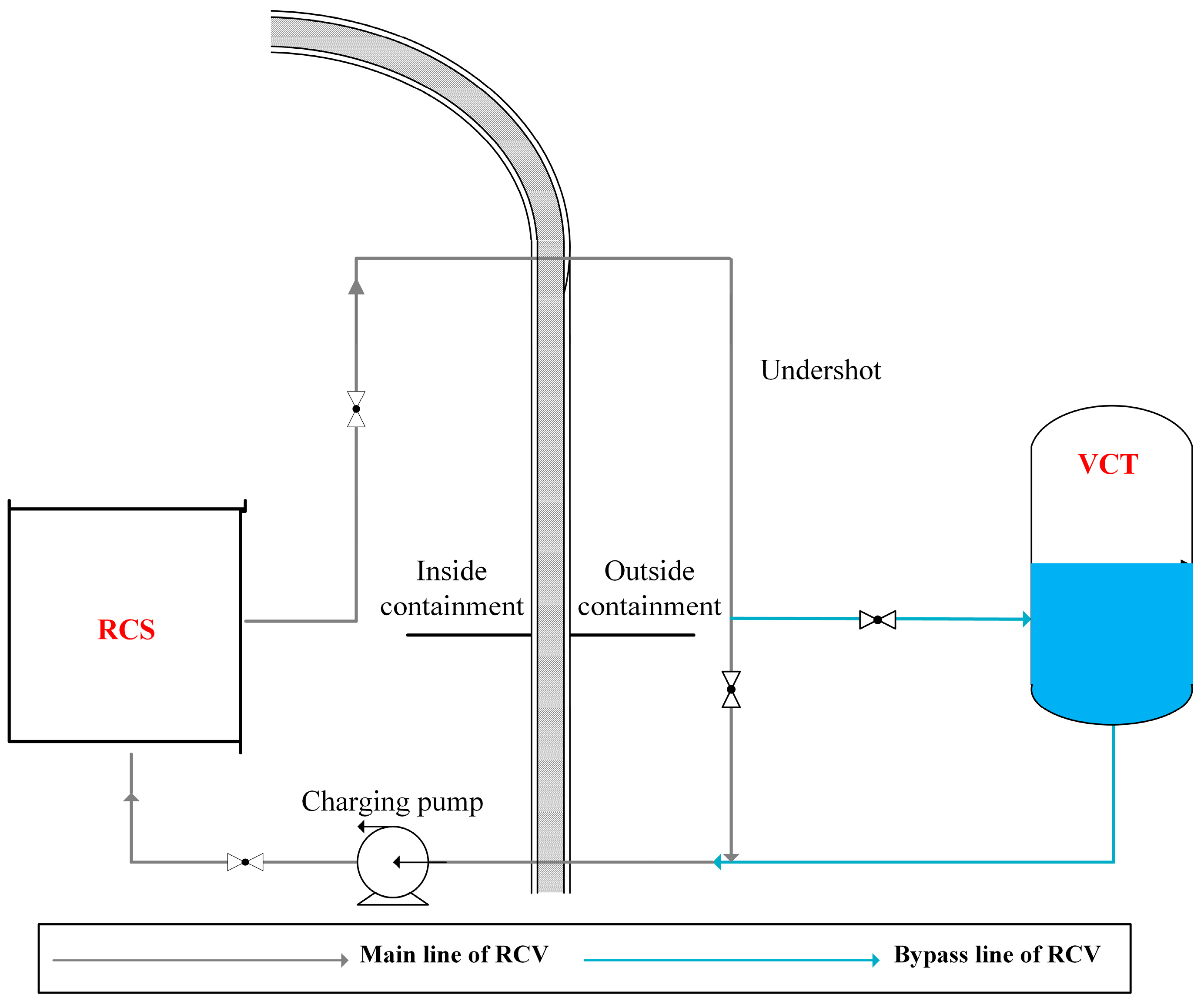
The primary circuit of a nuclear power plant is directly involved in heat exchange with the reactor core, which is filled with radioactive coolant. Therefore, the safety of the primary circuit of the nuclear power plant is important for the entire nuclear power plant. The chemical and volume control system (RCV) is installed in the primary circuit, and an essential component of the RCV system is the VCT, as shown in Figure 1 [1]. The VCT is used to capture and contain the underdrain stream and provide volume compensation for the coolant in the primary circuit. In addition, it serves as a high-level tank to supply a net positive draw-in pressure head for the top-fill pump. At the same time, the gas-phase volume in the upper portion of the VCT simultaneously functions as degasification and hydrogen addition. During normal operation of the nuclear power plant, the downdraft flow is ejected from the nozzle in the lower and middle parts of the VCT, and the fission gas is separated from the coolant. The shorter half-life fission gases decay away during the retention process in the VCT, while the longer half-life nuclides are removed less effectively. Therefore, hydrogen and nitrogen are used periodically in nuclear power plants for purging and carrying fission gas to the exhaust gas treatment system.
The upper part of the VCT is filled with nitrogen, and the lower part is the coolant for the primary circuit. The liquid-phase flow in the VCT is driven by the submerged jet of the lower drainage, and the mass transfer between the nitrogen and coolant occurs inside the VCT. When the solution in the VCT enters the primary circuit, the nitrogen dissolved in the primary circuit coolant is converted to the intermediate product 14N(n,p)14C by neutron bombardment. The dangerous radioactive element 14C, with a half-life of 5730 years, is further generated and will enter the atmosphere with the exhaust gas during blowdown. Under normal operating conditions at nuclear power plants, 14C is one of the airborne radionuclides that contributes the most to the public’s effective dose. 14C will be absorbed by the human body after entering the environment, and it poses a grave threat to human health. Moreover, the nitrogen gas entering the primary circuit is also easily precipitated near the core, which affects the stability of the flow and heat transfer. Just 1% of non-condensable gas can cause about 60% of heat transfer deterioration due to condensation heat transfer. Additionally, the convective heat transfer coefficient of gases is significantly lower than that of liquids. The localized deterioration of heat transfer can lead to additional thermal stresses in the primary circuit, as well as temperature fluctuations, which will accelerate the thermal fatigue of pipes. More than 3700 pipeline failure data have been recorded by the OECD/NEA OPED (OECD/NEA Piping Failure Data Exchange Project) from 321 nuclear power plants. During the 8300 reactor years of commercial operation, a total of 128 cases of thermal fatigue damage to pipes occurred, 63 of which resulted in coolant loss [2]. Therefore, it is important to study the gas–liquid mass transfer mechanism driven by submerged jets in the VCT and to analyze the influence law of different structural parameters on the gas–liquid mass transfer process for the safe and stable operation of nuclear power plants.
Currently, three main theoretical models have been developed for the study of gas–liquid mass transfer behavior:
- Two-film model;
The two-film model [3] considers the existence of a stable phase interface between the gas and liquid phases, with stable gas and liquid membranes on the gas and liquid sides, respectively. The mass transfer coefficient can be calculated by Equation (1).
where is the gas diffusion coefficient, and is the thickness of the liquid film.
- 2.
- Penetration model;
Unlike the two-film model [4], the penetration model assumes gas–liquid mass transfer is a dynamic process, rather than through a stagnant film. The fluid microelement from inside the liquid phase arrives at the gas–liquid interface and stays for a while to exchange substances with the gas phase. The mass transfer coefficient can be calculated by Equation (2).
where is the fluid microelement residence time, and is the circumference.
- 3.
- Surface renewal model;
The surface renewal model [5] is a development of the penetration model. The surface renewal model assumes that the renewal of the fluid microelement at the gas–liquid interface occurs continuously rather than every certain residence time. The age distribution function is introduced to describe it.
where is the age distribution function of the fluid microelement, is the surface renewal rate of the fluid microelement, and is the residence time. The mass transfer coefficient can be calculated by Equation (4).
At present, gas–liquid mass transfer studies are targeted at open channel flow, Oscillating Grid Turbulence (OGT), and natural convection. Oxygen was used as the gas working medium by Xu [6] to study the gas–liquid mass transfer under annular wind-shear open channel flow, where the liquid-phase flow rate ranges from 0 to 10.5 mL/s, and the air flow rate ranges from 3 to 7 m/s. Xu [6] investigated the mass transfer processes of liquid-phase absorption and gas release during gas–liquid co-current and counter-current flow. Turney [7] further conducted a comparative study of the surface dispersion model under wind-shear open channel flow and gas-phase stationary open channel flow, and a new model for mass transfer rate calculation was proposed by combining the surface dispersion model and the surface renewal model. Herlina [8] studied OGT gas–liquid interface mass transfer using oxygen for turbulent Reynolds numbers () between 260 and 780, focusing on the statistical parameters that determine the mass transfer process. The results showed that the gas transport process is controlled by the vorticity spectrum at different scales, and the higher the degree of turbulence, the stronger the effect of small vortices and the weaker the effect of large vortices. Jirka [9] studied the gas–liquid interface mass transfer under OGT and natural convection, focusing on the mass transfer mechanisms of both, and visualizing the concentration and turbulence fields.
Some scholars have studied the effect of vortex structure to better understand the role of the turbulent flow field on gas–liquid mass transfer. Lovatte [10] studied the gas–liquid interface mass transfer under open channel flow using the LES method to analyze the effect of the Reynolds number () on fluid flow and mass transfer, and the results showed that the vortex structure near the gas–liquid interface is the direct cause that drives fluid micro-element replacement. Nagaosa [11] investigated the time scale of turbulent vortices controlling scalar transport and compared and analyzed it with the fluctuation period of gas concentration. Dani [12] found that the rate of gas–liquid mass transfer is deeply influenced by the presence and size of vortices.
Turbulent flow fields exhibit different characteristics in different application scenarios, which have significant effects on gas–liquid mass transfer, such as fluid thermal stratification, surface contamination, the influence of water plants and wind waves, etc. Dong [13] and Teraoka [14] investigated the effect of the thermal stratification phenomenon on mass transfer due to uneven temperature distribution, and DNS simulations of open channel flow in the presence of thermal stratification were also carried out at a large range of Richardson () numbers to investigate the liquid-phase turbulence characteristics and the dependence of the Nusselt number on the . Teraoka [14] carried out DNS calculations of open channel flow in the presence of thermal stratification and analyzed the effect of thermal stratification on the turbulence characteristics at the water surface. The results showed that the surface dispersion and the magnitude of heat flux near the gas–liquid interface are determined by the layered structure of the liquid phase. Herlina [15,16] and Khakpour [17], who focused on the effect of surfactant contamination on mass transfer, concluded that when the gas–liquid interface is heavily contaminated, its properties will converge to the wall (no-slip boundary conditions). Herlina [15,16] pointed out that the gas transport velocity was reduced by 80% for surface contamination at , while the concentration fluctuations near the interface were significantly reduced. Khakpour [17] showed that the interfacial scalar transfer was mainly affected by the surfactant through both short-wave suppression and updraft suppression effects. Lu [18] investigated the effect of the presence of vegetation on the turbulent structure and solute mixing; analyzed turbulence characteristics, such as vortex length scale and Reynolds stress, in conjunction with vegetation density; and quantified the variation of the concentration distribution along the flow direction with the vegetation density. Huang [19] investigated the effect of separate turbulent pulsations on mass transfer within biofilms and found that an increase in the intensity of turbulent pulsations resulted in significant stratification of the permeate velocity gradient in the biofilm, which enhanced convective mass transfer.
At present, there are few studies on the gas–liquid mass transfer behavior driven by submerged jets, and there are even fewer studies on the influence of geometric structure on the behavior. In this paper, a novel mass transfer model capable of accurately simulating gas–liquid mass transfer phenomena is developed that combines a surface dispersion model with a CFD model and can well simulate the process of the gas phase entering the liquid phase. The gas–liquid mass transfer mechanism driven by a submerged jet is investigated using this model. On this basis, the influence of structural parameters of the VCT on gas–liquid mass transfer behavior under the submerged jet drive is investigated. This study has significant application value for the design, operation, and improvement of the VCT and similar facilities in nuclear power plants.
2. Numerical Simulation Study
2.1. Geometric Model
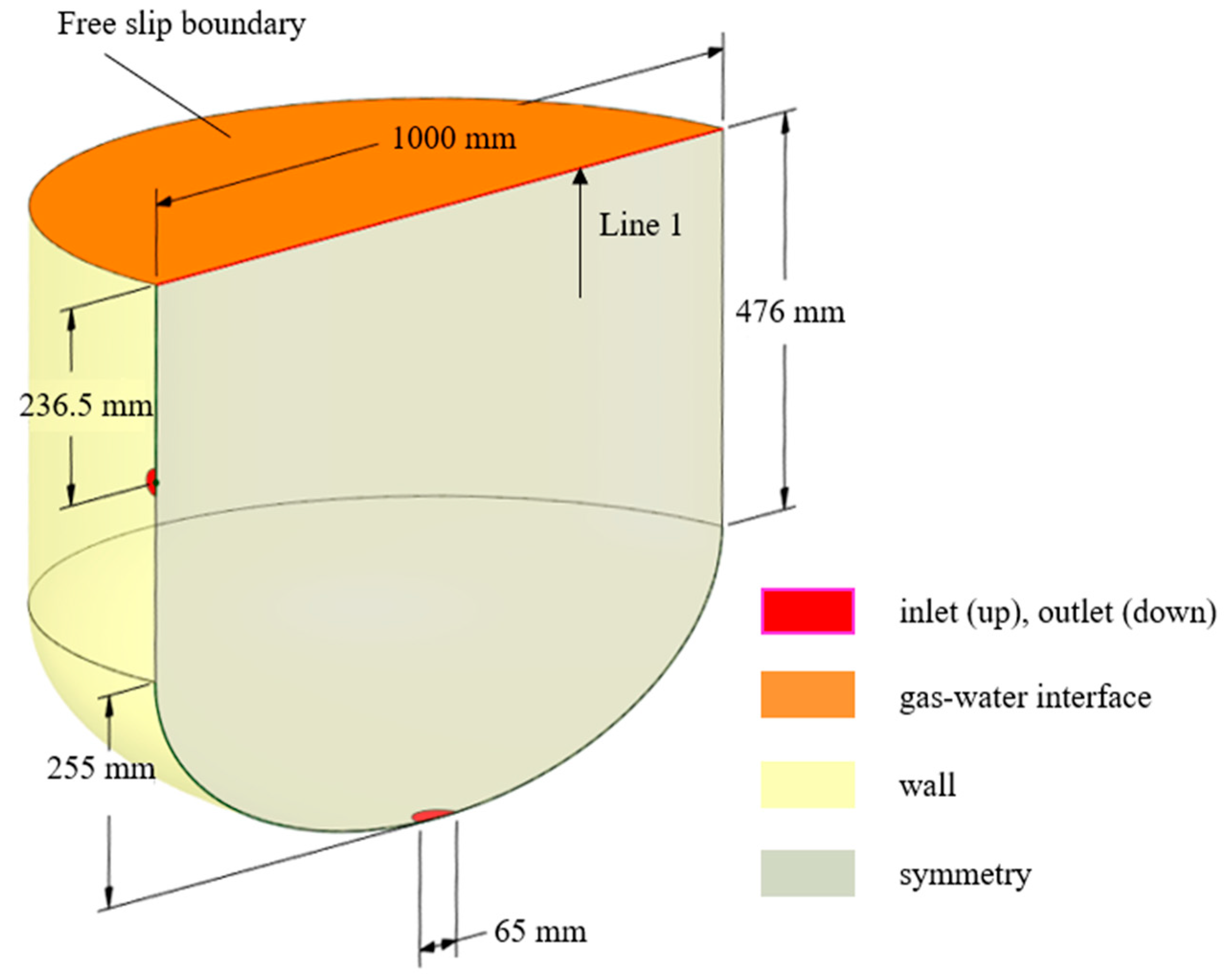
In this study, the geometric model was performed based on the actual structure of the primary circuit VCT in the nuclear power plant. For low-solubility gases, such as nitrogen and oxygen, the gas–liquid mass transfer process is primarily determined by the fluid dynamics on the liquid side, and the mass transfer process is less affected by the deformation of the gas–liquid interface [6], and the gas-phase part and the liquid surface undulation are ignored in most studies. Therefore, in this paper, only the liquid-phase part was geometrically modeled, and the gas–liquid interface was assumed to be a flat interface. Due to the high symmetry of the VCT structure, the symmetry plane was used as the boundary, and half of the study object was geometrically modeled to save computational time and cost. The geometric model is shown in Figure 2. On line 1, 1000 monitoring points are configured for data monitoring.
For non-stationary problems with transient solutions, boundary conditions need to be specified. Five common boundary condition settings are provided in Fluent, including the entrance boundary condition, the exit boundary condition, the solid wall boundary, the symmetric boundary condition, and the periodic boundary condition. The boundary condition settings in this paper are shown in Table 1. The mathematical expression of the boundary conditions is as follows:
For the inlet,
where is the partial velocity along the coordinate axis y direction, is the partial velocity along the coordinate axis z direction.
For the wall surface,
where is the partial velocity along the coordinate axis x direction, is the normal vector of the plane, is the oxygen concentration.
For the symmetrical surface,
The numerical simulation conditions are shown in Table 2. Each numerical simulation case is paired with an experimental case for validation. Take the case CFD-H1D2Q1 as an example, the symbol CFD represents the numerical simulation, H1 represents the first level of the horizontal inlet height, D2 represents the second level of the horizontal jet diameter, and Q1 represents the first level of the horizontal inlet flow rate. The Reynolds number range for the numerical simulation conditions is .
2.2. Governing Equation
In this simulation, the experimental system was assumed to have no heat exchange with the outside world. The basic governing equations of the numerical simulation are as follows:
Equation (11) is the continuity equation, Equation (12) is the Navier–Stokes equation, and Equation (13) is the transport equation for oxygen concentration , where takes values in the range of 1, 2, and 3; represents the coordinate axis direction; is the fluid density; is the mass source term added to the liquid phase; is the partial velocity along the coordinate axis direction; is the static pressure; is stress tensor; is the component of gravitational acceleration along the coordinate axis direction; is the external force term; is the mass diffusion coefficient; is the turbulent Schmidt number; is the turbulent viscosity; and is the component for the mass source term. In this study, there is . We have treated the buoyancy term based on Boussinesq approximation in order to reduce the nonlinearity of the system. The specific mathematical expression is as follows:
where is the reference density, is the oxygen concentration corresponding to the reference density, is the expansion coefficient.
The Reynolds stress term is introduced into the control equation in the RANS method, resulting in the equation no longer being closed. Therefore, different turbulence models are developed to make the set of control equations closed. In this paper, the standard turbulence model was selected for the calculations. This model has good robustness, economy, and reasonable accuracy for most turbulent flows and is one of the most widely used turbulence models in industrial flow and heat transfer simulations. The transport equation for the standard turbulence model is as follows:
In the two equations above, represents the generation of turbulence kinetic energy due to the mean velocity gradients, is the generation of turbulence kinetic energy due to buoyancy, represents the contribution of the fluctuating dilatation in compressible turbulence to the overall dissipation rate. , and are constants. and are the turbulent Prandtl numbers for and , respectively. and are user-defined source terms.
2.3. Mass Transfer Model
The User Defined Function (UDF) is provided in ANSYS Fluent, which can be dynamically loaded with the ANSYS Fluent solver to enhance its standard functionality. In this section, the UDF is used to couple the surface dispersion model and the CFD model to simulate the process of gas entering the liquid phase.
According to the gas–liquid mass transfer theory equation, the gas mass source term entering the liquid phase through the gas–liquid interface per unit time is shown in Equation (17):
where is the mass transfer coefficient; is the saturation concentration of the gas at that temperature and pressure; is the concentration of the gas in the liquid-phase subject away from the gas–liquid interface; and are the area of the gas–liquid interface and the volume of the liquid phase involved in mass transfer, respectively. According to the surface dispersion theory, is related to the surface dispersion near the gas–liquid interface and the diffusion coefficient [5,8], as shown in Equation (18).
where is an empirical coefficient taking values from 0.2 to 0.7 [20,21]. is the diffusion coefficient as a function of temperature. is the root mean square (RMS) of the surface dispersion , defined as follows [21,22]:
In this paper, is calculated from the turbulent flow field in the range of 7 mm near the gas–liquid interface. The vertical pulsation velocity at the gas–liquid interface decays to zero, and the pulsation velocity derivative is discretized as follows:
where is the root mean square of the vertical pulsation velocity at 7 mm from the free liquid surface, and is the distance of the grid from the gas–liquid interface (7 mm).
2.4. Physical Property and Calculation Method
Due to the constant temperature and pressure of the working fluid, the physical properties remain constant during the simulation. The properties used in the simulation are derived from the Refprop software version 9.1. The properties are calculated with double precision, and the solution settings are as follows:
- (1)
- Water is considered an incompressible fluid in the calculation, and the pressure-based solver is chosen for the solution.
- (2)
- The PISO algorithm is used to solve the Navier–Stokes equations. The PISO algorithm has high accuracy and computational efficiency in the solution of transient problems. In this paper, the energy equation is not solved, and the time step is considered converged when the residuals of the remaining equations are less than 10−5. The second-order windward method is used to perform spatial discretization of the governing equations.
- (3)
- Transient calculations are employed. A variable time propulsion step size ranging from 0.01 s to 0.1 s is adopted based on the Courant Friedrichs Lewy condition to maintain numerical stability [23]. The results are considered converged when the relative residuals of mass conservation, momentum conservation, and component transport equations are less than 10−4.
2.5. Grid Convergence Validation
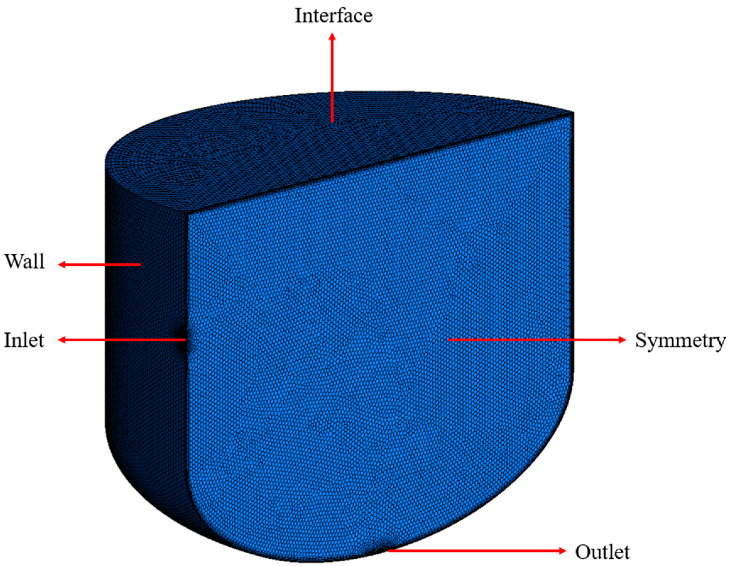
Several wall function models are available in ANSYS FLUENT, such as Standard Wall Function, Scalable Wall Functions, and Non-Equilibrium Function models. Different wall function models have different requirements for the mesh , and the selected wall function model needs to be considered when dividing the mesh. In this paper, the Scalable Wall Functions model was selected because it can provide consistent solutions for any refinement of the mesh and prevent the deterioration of the computational results when . To ensure the mesh quality and save computational cost and time, the hexahedral mesh was used for meshing, and the mesh was encrypted at the boundary layer and gas–liquid interface, with a maximum mesh skew rate of less than 0.5. The mesh is of high quality. The grid is shown in Figure 3.
The number of grids is also one of the important factors to be considered. An insufficient number of grids will result in insufficient computational accuracy, while too many grids will increase the computational cost and computational cycle; thus, grid convergence verification is required. GCI is a widely used quantitative measure of lattice convergence, and the specific procedure of GCI is referred to by Sosnowski [24] and Roache [25]. We used three meshes for the grid convergence index (GCI). All the values of the quantities are listed in Table 3. The obtained results indicate the mesh convergence with the GCI equal to 0.42%.
3. Experimental Study
3.1. Experimental Method
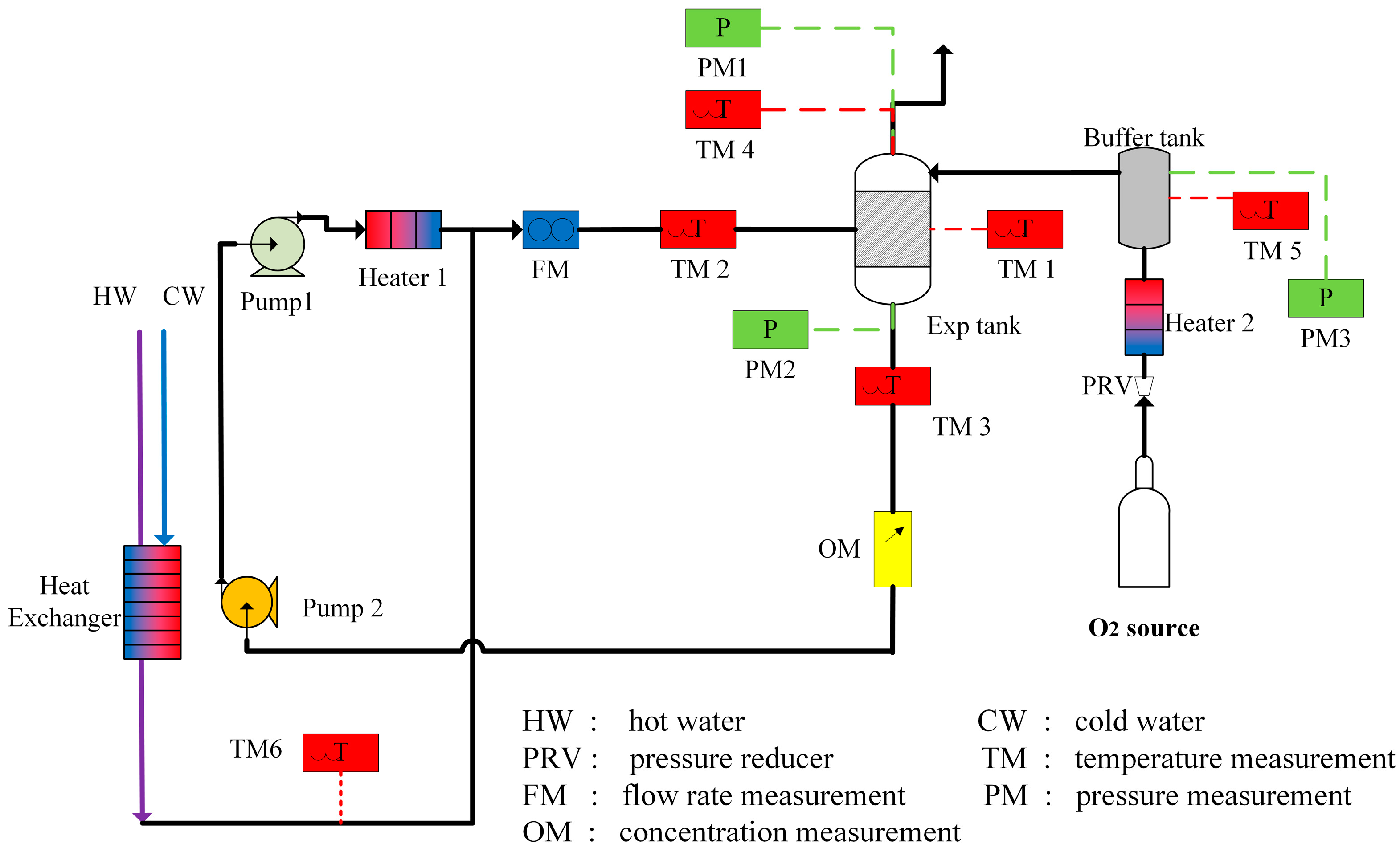
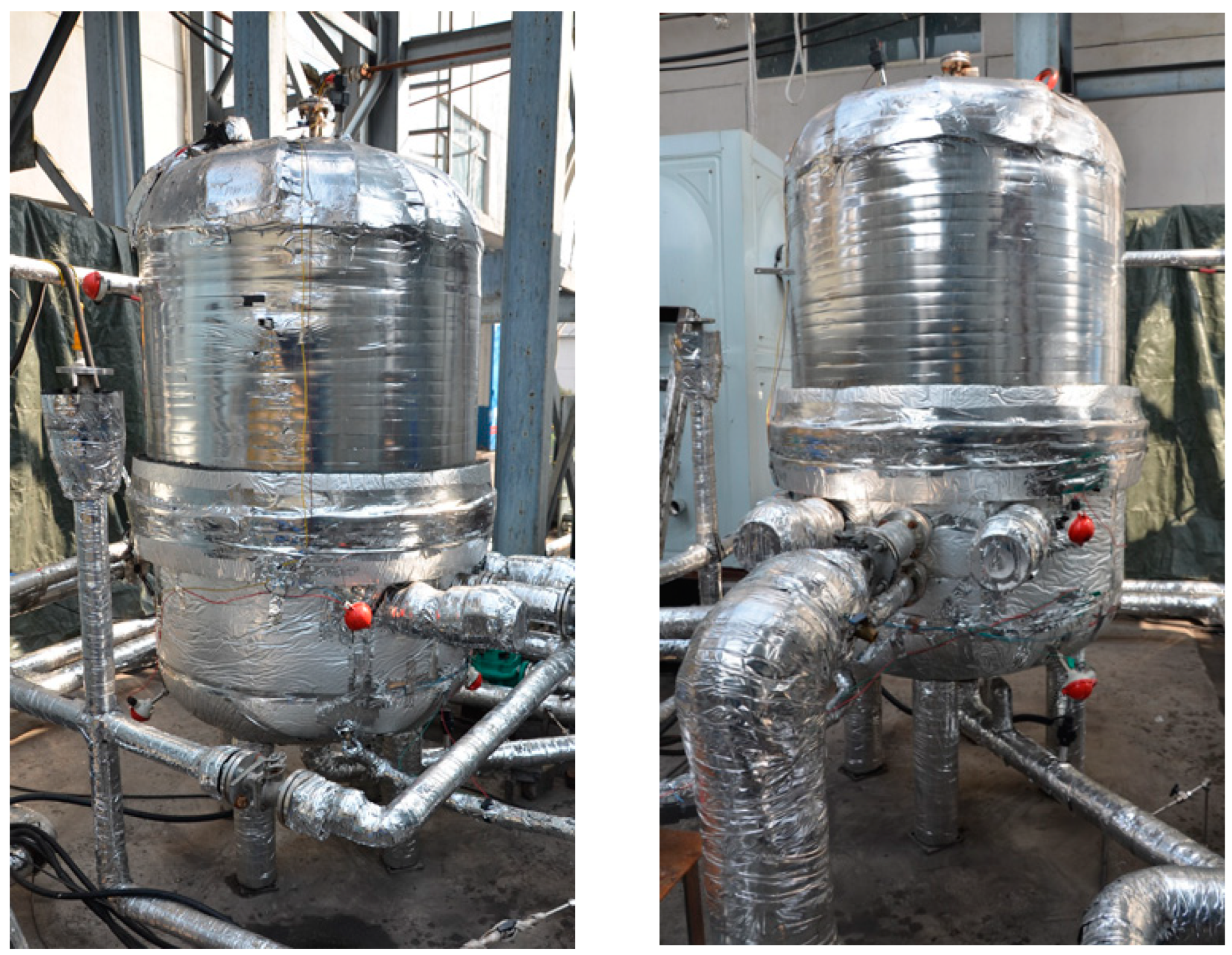
Validation experiments were conducted to verify the accuracy of the numerical model. The specific steps of the experiments were described in detail in a previous study [26], and this paper provides only a summary. The validation experimental system is shown in Figure 4, and the experimental site is shown in Figure 5. The experimental system mainly consists of the experimental body, water supply, air supply system, parameter control system, experimental measurement, and data collection system. After the experiment started, high-temperature water was introduced by the water supply system and cooled to the experimental temperature by the plate heat exchanger in the parameter control system to obtain the liquid-phase work mass. The room-temperature gas phase was introduced by the gas supply system and heated to the experimental temperature by the heater in the parameter control system to obtain the gas-phase work. The liquid-phase mass was driven by a pump to create a circulating flow in the circuit when the experiment started. Oxygen was chosen for the experiments because the measurement method for nitrogen was not mature.
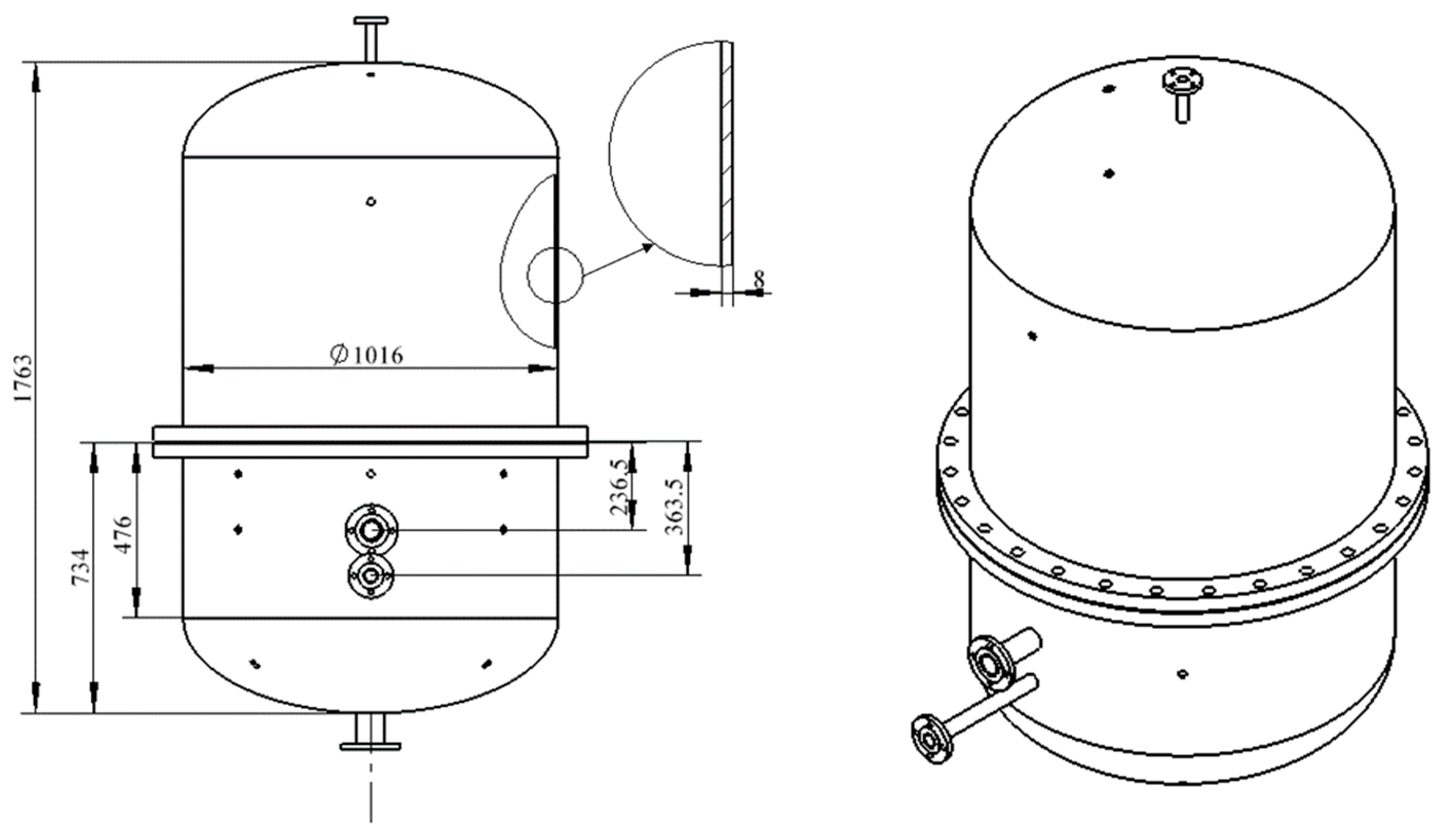
The experimental object was the VCT with the structure shown in Figure 6. For better pressure bearing, 304 stainless steel was chosen as the material. The internal diameter of the tank was 1.0 m, the height of the tank was 1.763 m (excluding the support), and the wall thickness of all walls of the tank was 8 mm. The upper and lower heads of the tank were DN1000 EHA standard elliptical heads with a volume of about 1.24 m3. The tank was divided into two parts, which were connected by DN1000 flanges. During the experiment, the lower part of the tank was filled with liquid-phase work water with a height of 0.476 m. The bottom was equipped with a water outlet, and the outlet pipe was a DN65 standard pipe with a wall thickness of 3 mm, which was connected with the pipe by a flange. With the flange surface as the boundary, the upper part of the VCT was filled with O2, and the height of the cylindrical part was 0.771 m. The top had an inlet port, and the inlet pipe was a DN20 standard pipe with a wall thickness of 3 mm.
To prevent the experiments from being affected by the ambient temperature, a 50 mm thick layer of rubber foam insulation material was uniformly wrapped around the outside of the tank. A through-hole was installed at the top of the tank for the installation of a pressure transmitter to measure the pressure inside the tank. A through-hole was located in the upper tank at 0.371 m from the lower edge of the upper head for the installation of a Pt100 RTD to measure the gas-phase temperature. The lower tank was set out symmetrically with through-holes, 4 holes per layer, 3 layers in total, for the installation of the RTD for measuring the liquid-phase temperature. Two jet inlets of different heights were set up on the tank. The upper inlet was the main inlet, with an inner diameter of 49 mm and a height of 0.2365 m from the upper and lower tank flanges, and the lower inlet was a secondary inlet, with a standard DN32 pipe of 3 mm wall thickness and a height of 127 mm from the main inlet to investigate the effect of jet height on the mass transfer at the gas–liquid interface. The main inlet was designed as a removable structure for simple replacement and was used to investigate the influence of jet diameter on the gas–liquid interface mass transfer.
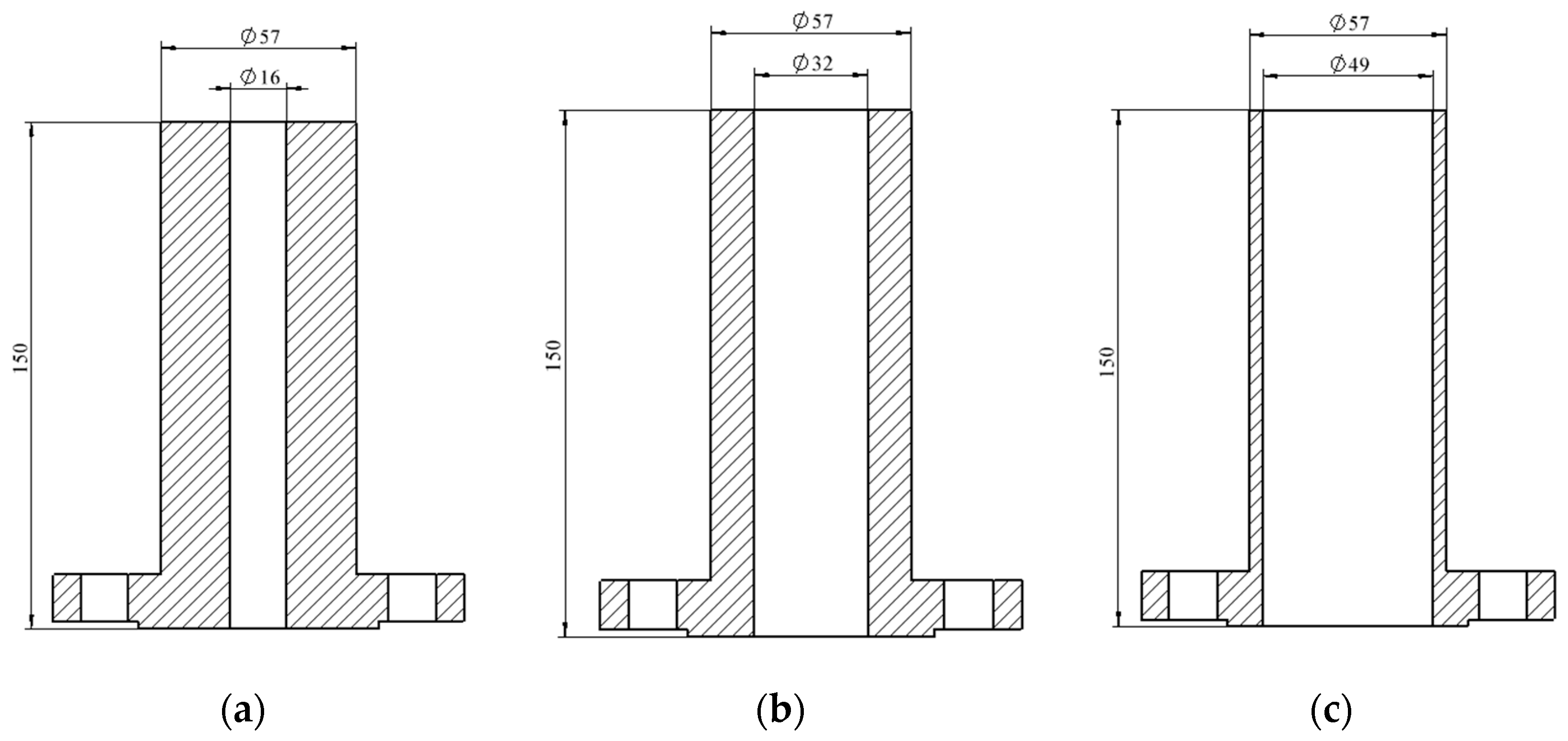
As shown in Figure 7, there are 3 types of inlet pipes made of 304 stainless steel. Tube (a) has an outside diameter of 57 mm and an inside diameter of 16 mm. Tube (b) has an outside diameter of 57 mm and an inside diameter of 32 mm. Tube (c) has an outside diameter of 57 mm and an inside diameter of 49 mm. During the experiment, different inlet tubes were inserted into the main inlet, and the gap between the inlet tube and the main inlet was filled with filling material.
3.2. Operating Condition
In addition to the experiments for reproducing and verifying the numerical simulation conditions, extended experiments were conducted. The experimental working conditions are shown in Table 4.
4. Results and Discussion
4.1. Mixing Mechanism
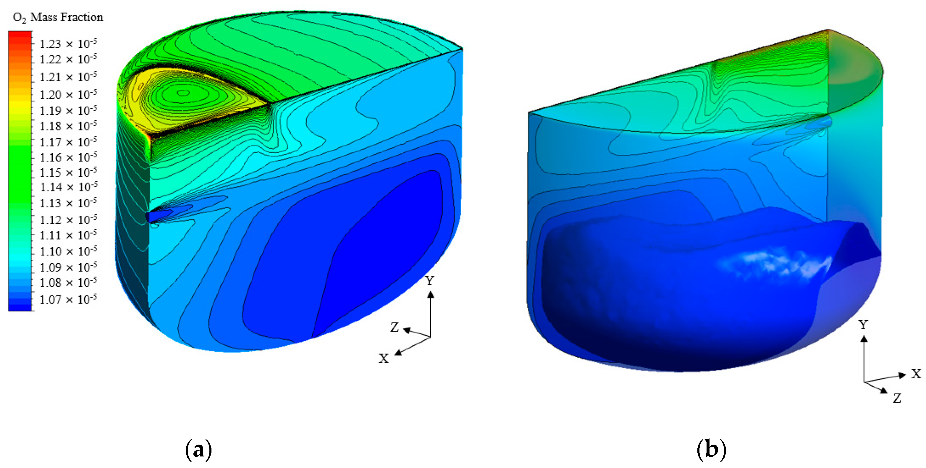
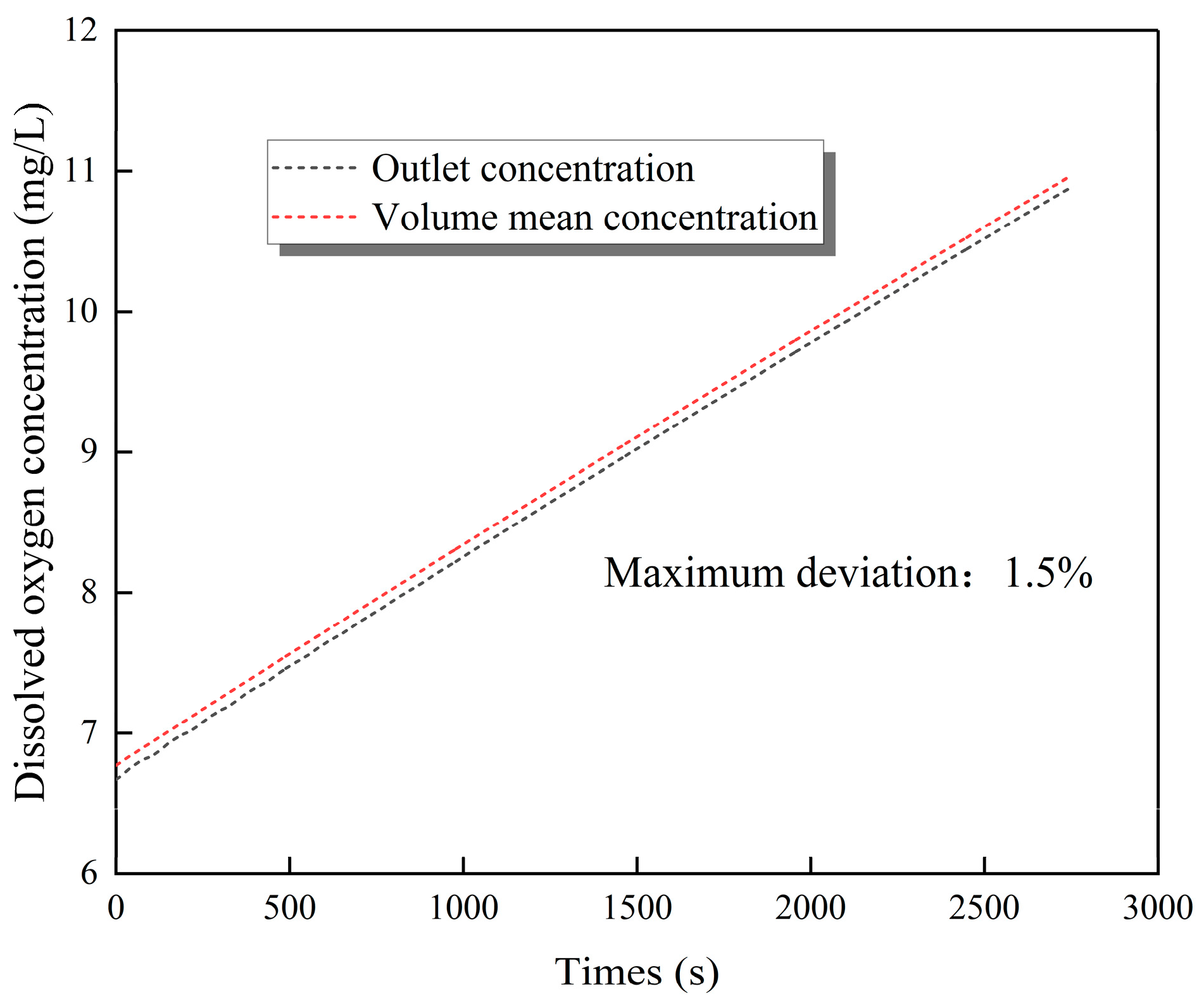
The baseline operating condition CFD-H1D2Q1 was chosen for analysis. The blue surface shown in Figure 8b is a surface of equal concentration, where the concentration on this surface is equal to the outlet concentration. The concentration deviation below the surface of equal concentration is less than 1%, and the concentration can be considered uniform; thus, the outlet concentration is equal to the bulk concentration . As also shown in Figure 9, the maximum deviation of the outlet concentration curve from the volume average concentration is 1.5%, and can be approximated as equal to .
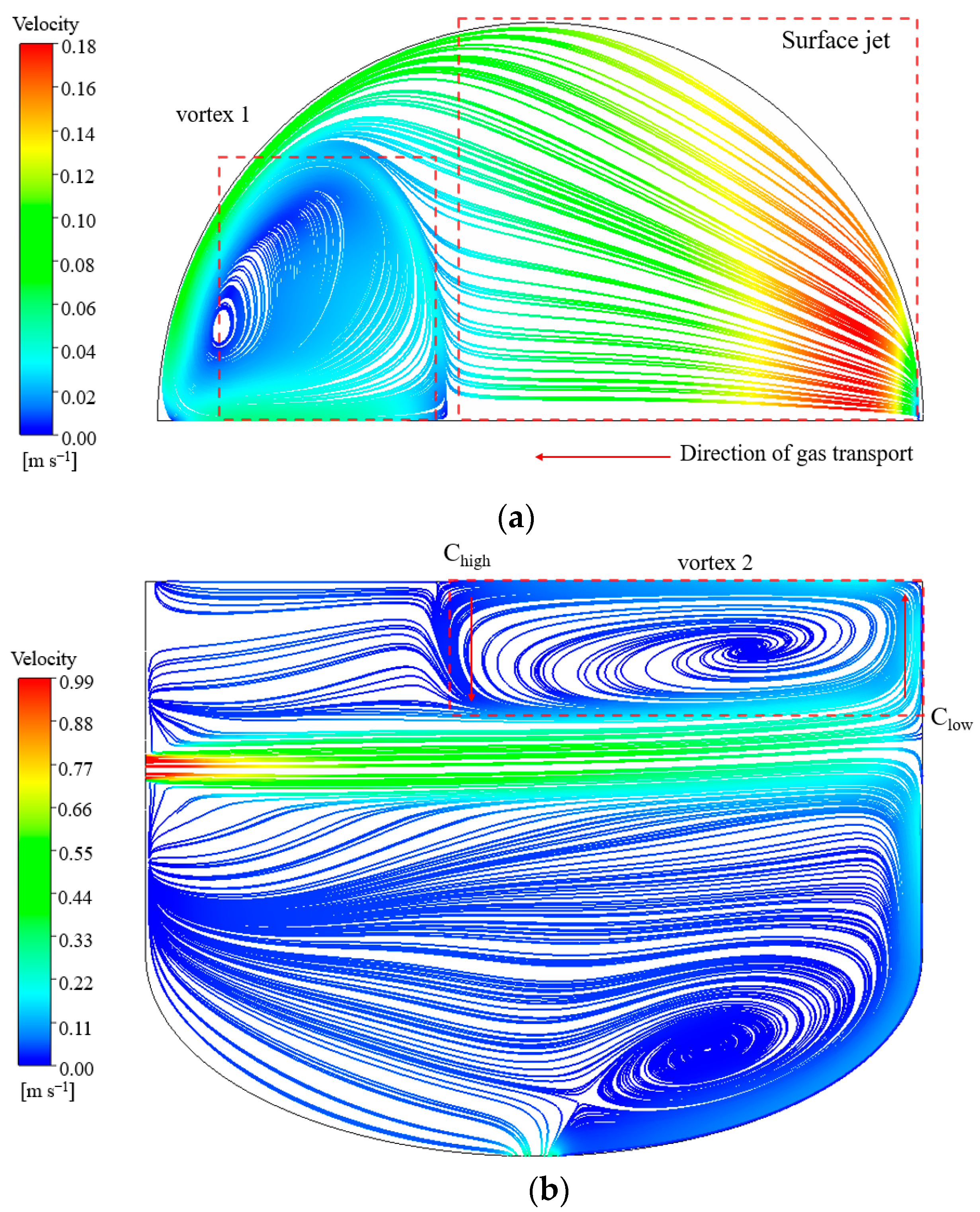
The distribution of dissolved oxygen concentration in the tank is shown in Figure 8a. It can be seen from Figure 8 that an obvious high-concentration region is formed at the upper part of the jet inlet end, and the highest dissolved oxygen concentration in the whole tank appears directly above the jet inlet. This is because this region is located downstream of the surface jet, and the gas entering the liquid phase from the gas-liquid interface in Figure 8a is borne by the surface jet, transported along the flow direction of the surface jet (positive direction of the x-axis) and accumulates. A circular concentration gradient distribution in the high-concentration region is also observed in Figure 8a, which is associated with the vortex structure of the flow field in the high-concentration region. The high-concentration fluid near the gas-liquid interface is swirled by vortex 1, and the swirling effect gradually decreases outward along the center of the vortex, forming an annular concentration gradient structure. Vortex 1 is formed when the surface jet generated along the vertical wall collides directly above the jet inlet. The numerical simulation only selected half of the VCT for the study, and there are two double vortex structures in the VCT with the xy plane where the centerline of the jet inlet is located as the symmetry plane.
The low gas concentration near the outlet of the VCT leads to a cone-shaped low-concentration region at the inlet of the VCT, and the concentration of the low-concentration fluid injected from the inlet increases steadily along the jet flow. Vortex 2 is formed above the end of the jet (Figure 10b), and the high-concentration fluid near the gas-liquid interface is displaced to the jet path by vortex 2 and mixed with the low-concentration fluid in the jet path. And subsequently, the mixed low-concentration fluid is displaced to the vicinity of the gas-liquid interface for mass transfer, resulting in the vortex-like concentration distribution at the corresponding location in Figure 10a.
In summary, the gas–liquid interface in the VCT is influenced by three macroscopic flow field structures. The first is the coiling and drawing effect of the double-vortex structure at the upper part of the jet inlet on the fluid near the gas–liquid interface. The second is the continuous renewal effect of the surface jet at the gas–liquid interface on the upstream high-concentration fluid. The third is the mass exchange between the fluid with a high concentration at the gas–liquid interface and the fluid with a low concentration at the end of the jet, which is caused by the vortex at the end of the jet. Obviously, the greater the renewal effect on the fluid near the gas–liquid interface, the greater the gas–liquid mass transfer effect between the two phases.
4.2. Comparison of Experimental Results with Numerical Results
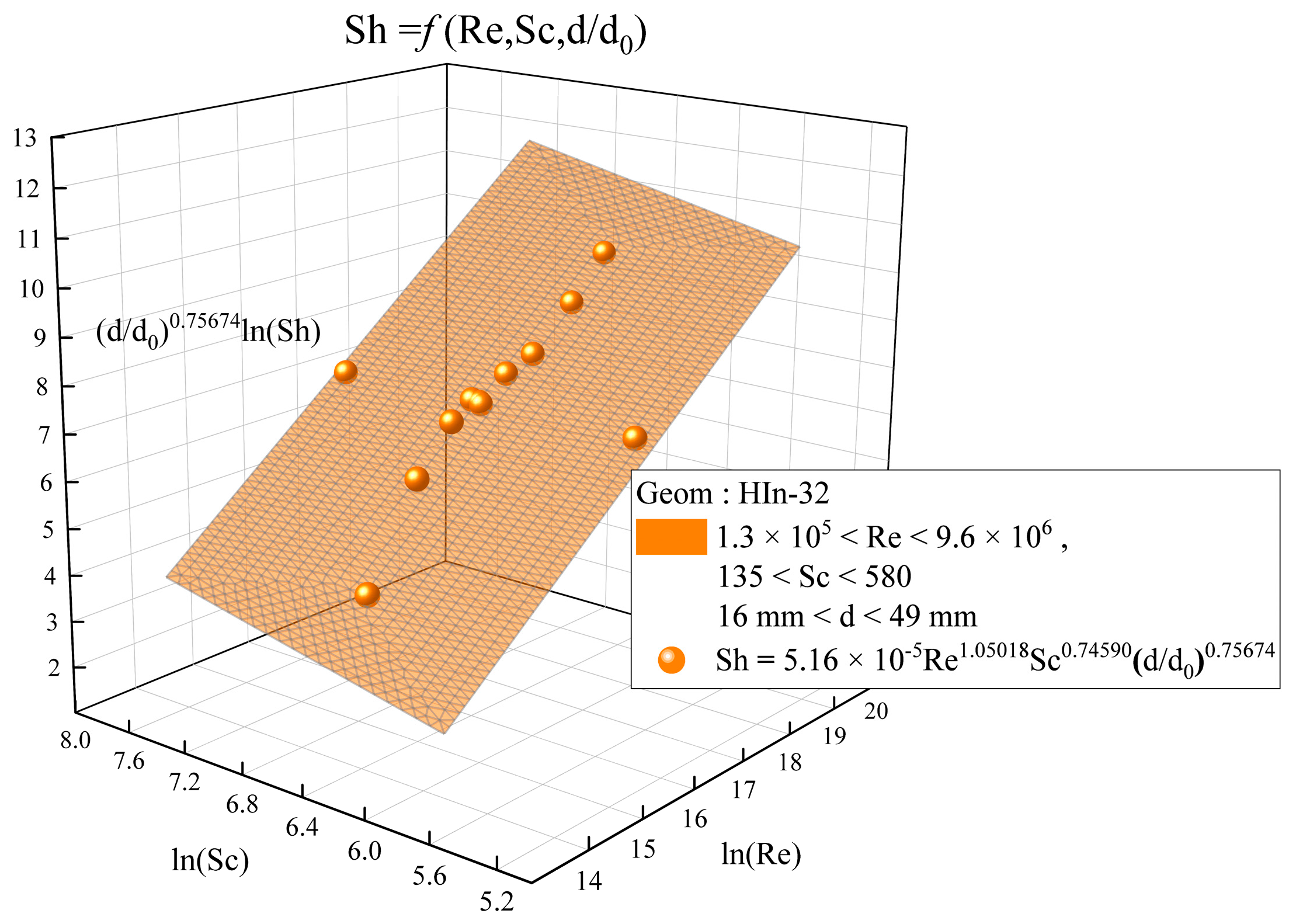
For the gas–liquid interface mass transfer behavior under various geometries and operating conditions, the dimensionless mass transfer coefficient () is closely related to the Reynolds number () and the Schmidt number (). For the same geometry, there is a unique mathematical relationship among the , the , and the under different operating conditions. After all the experimental data are fitted as shown in Figure 11, the following relationship is obtained:
The maximum deviation of Equation (21) is 22%, and the applicable range is .
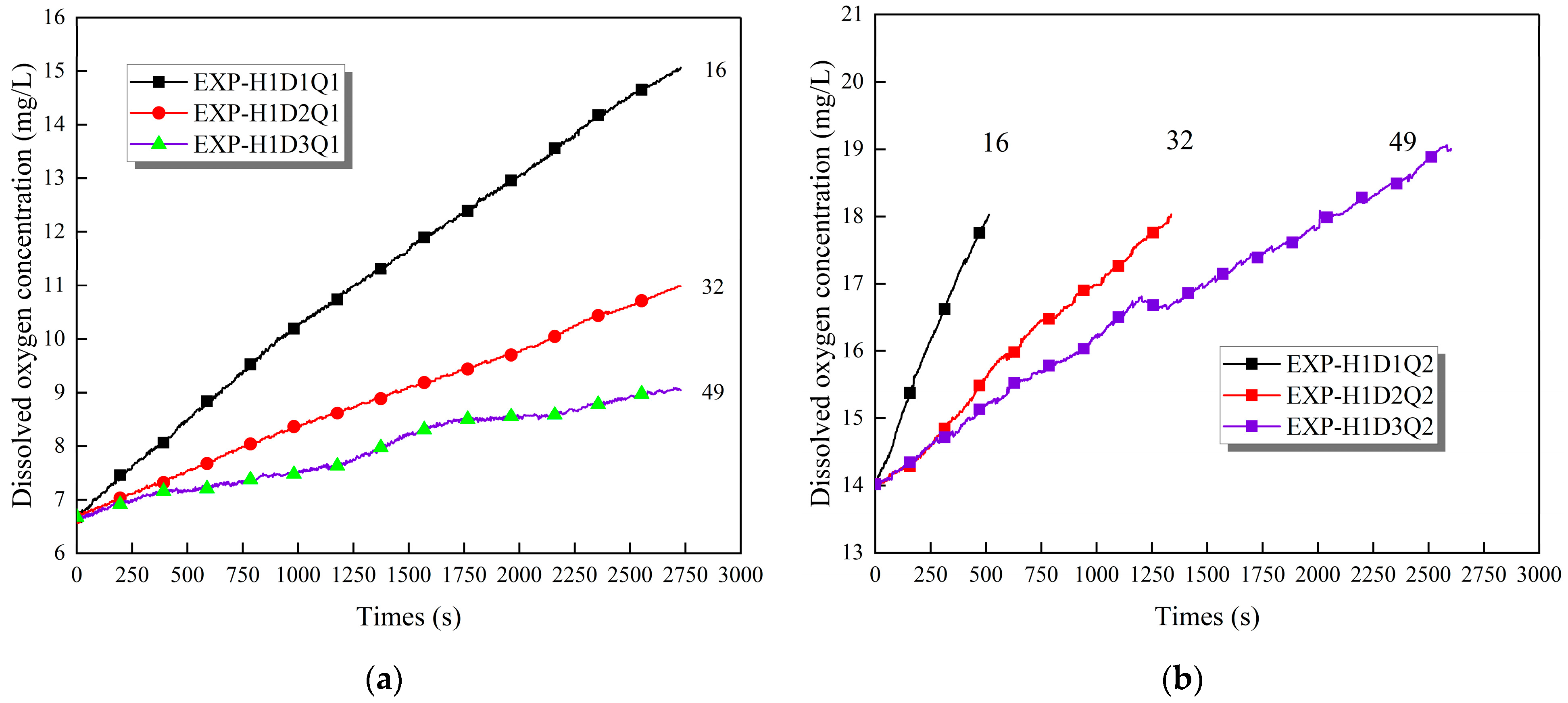
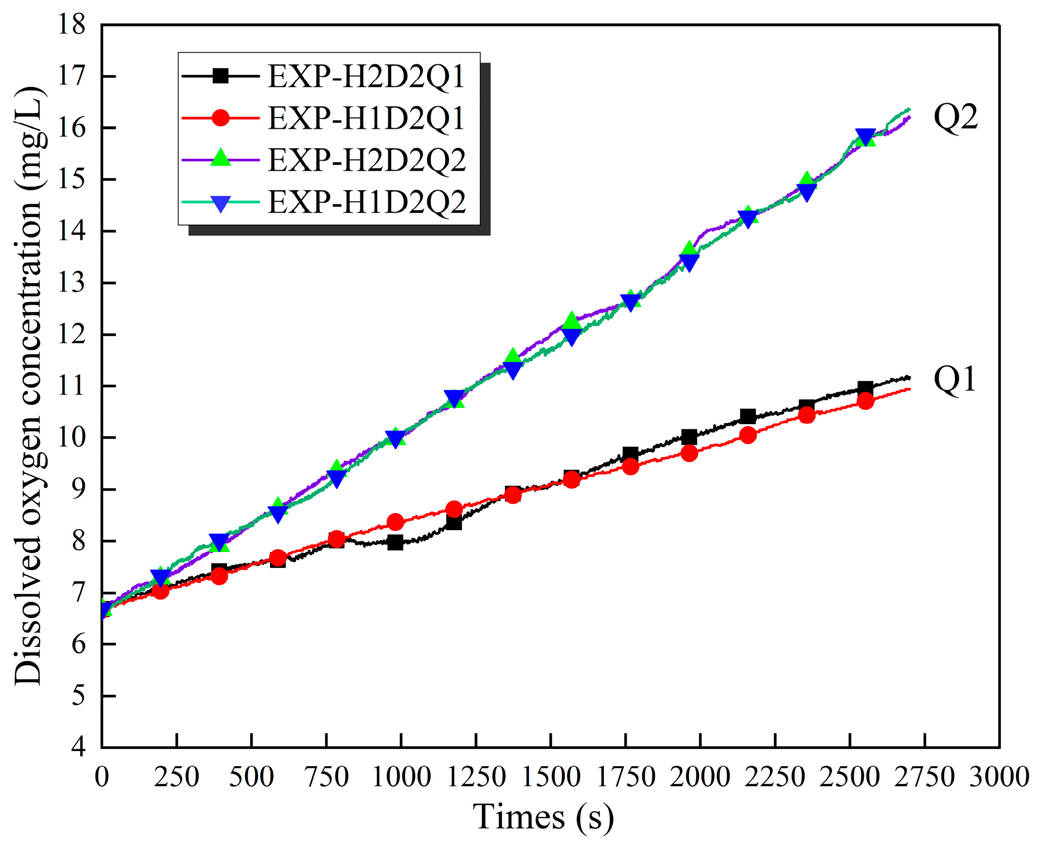
Figure 12 shows the variation of dissolved oxygen concentration curves at the outlet of the VCT for different jet diameters. It can be seen from Figure 12 that the dissolved oxygen concentration at the outlet of the VCT increases significantly quicker as the jet diameter decreases. Moreover, observing the experimental data of two different baseline conditions in Figure 12a,b, it is found that the change of the dissolved oxygen concentration curve brought by the change of the tube diameter has a strong regularity. The relative change in the mass transfer coefficient for the 2 experiments differs by 17% when the tube diameter is changed from 32 mm to 16 mm. The relative change in the mass transfer coefficient between the 2 groups of experiments is 8% when the pipe diameter is changed from 32 mm to 49 mm, where the relative change is calculated according to the following equation.
Figure 13 shows the concentration curves of dissolved oxygen at different jet heights. Figure 13 shows that the dissolved oxygen concentration curves for different flow rates differ significantly, but the curves for the same flow rate and different jet heights do not differ significantly. The jet height has no significant effect on the mass transfer flux or mass transfer coefficient at the gas–liquid interface. In the following, the mechanism will be analyzed in great detail.
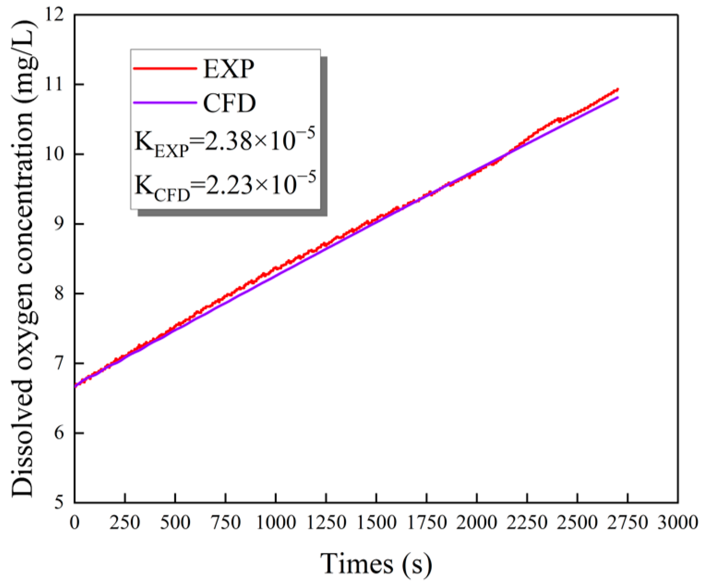
As shown in Figure 14, the numerical simulation results are compared with the experimental results. The selected data in the figure are the concentration of dissolved oxygen at the outlet, which is the primary concern, and the comparison reveals that the curve of the numerical simulation results closely matches the curve of the experimental data. The experimental mass transfer coefficient and numerical simulation mass transfer coefficient are also compared, and it is found that the maximum deviation between them was 6.55%, which is in acceptable agreement. The reasonableness and accuracy of the numerical model are verified.
4.3. Effect of Jet Diameter on Mass Transfer Process
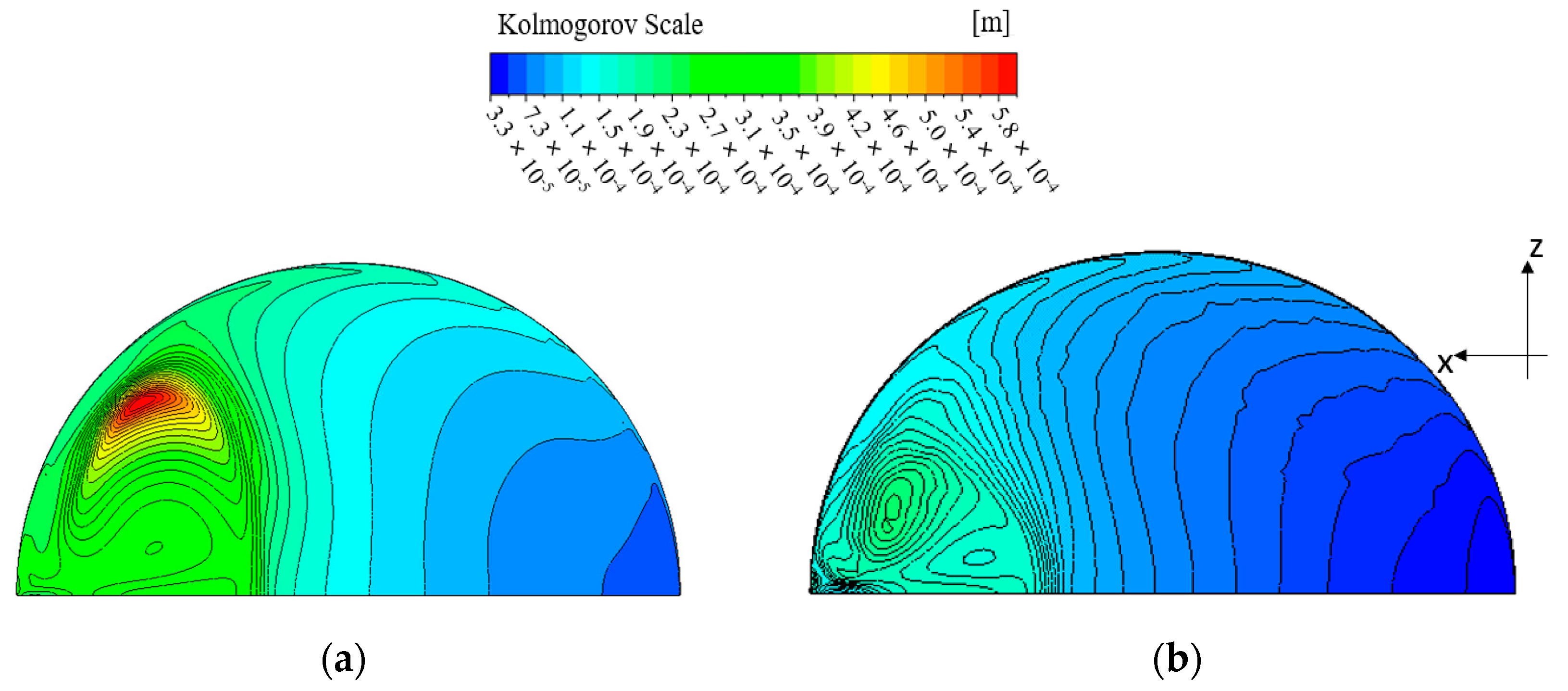
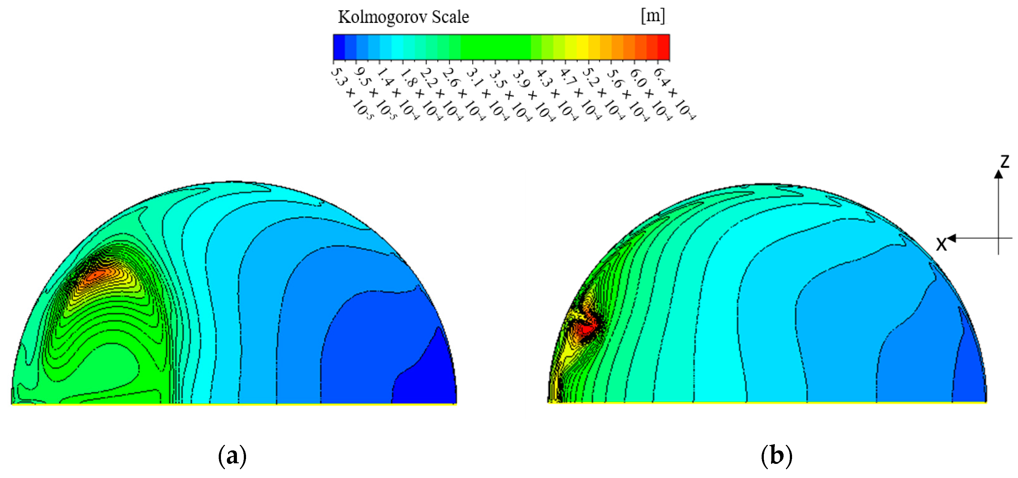
The distribution of Kolmogorov scales at the gas–liquid interface is depicted in Figure 15. The Kolmogorov scale is determined by the turbulent dissipation rate and the fluid kinematic viscosity , which are calculated according to the following equation [27]:
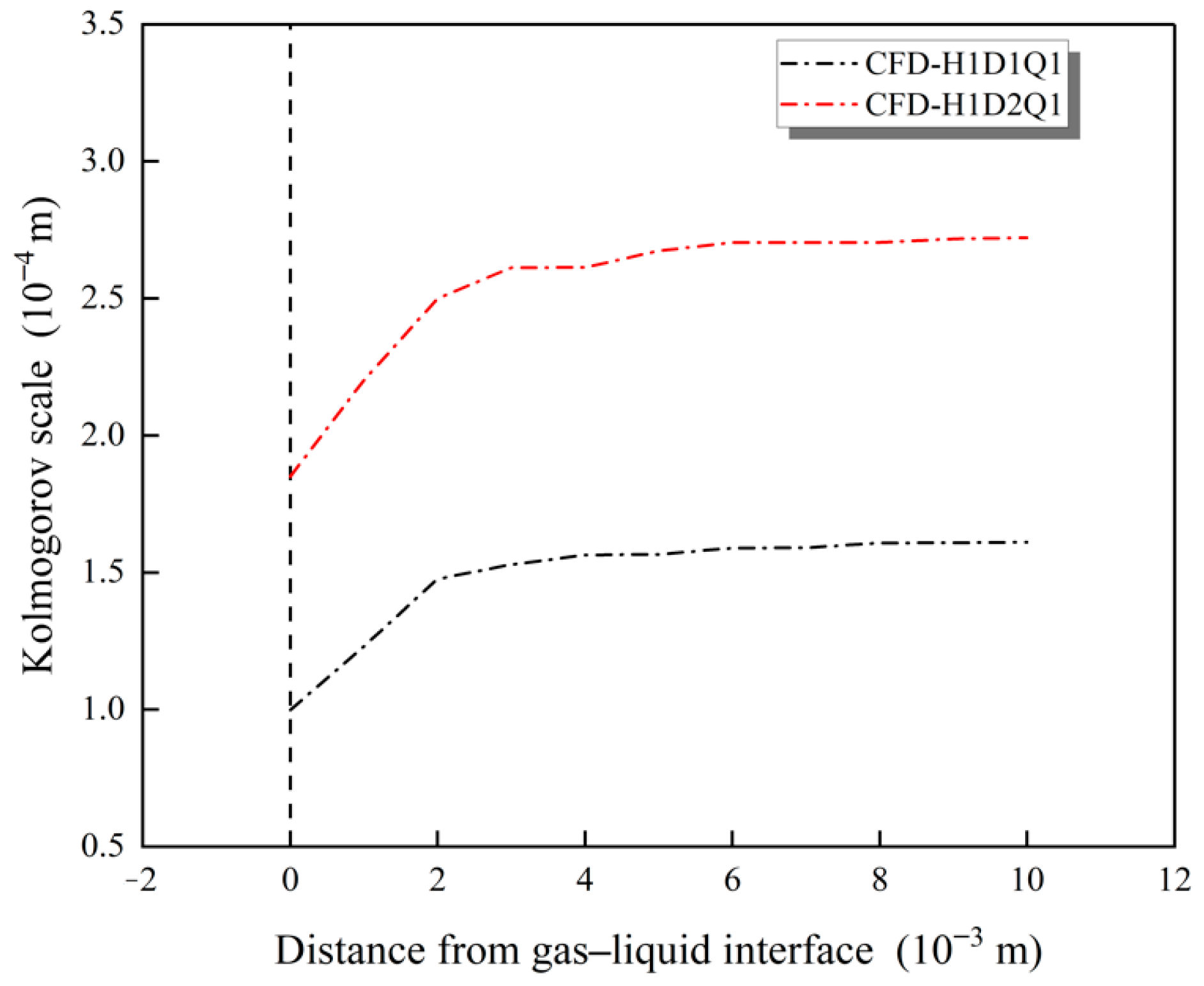
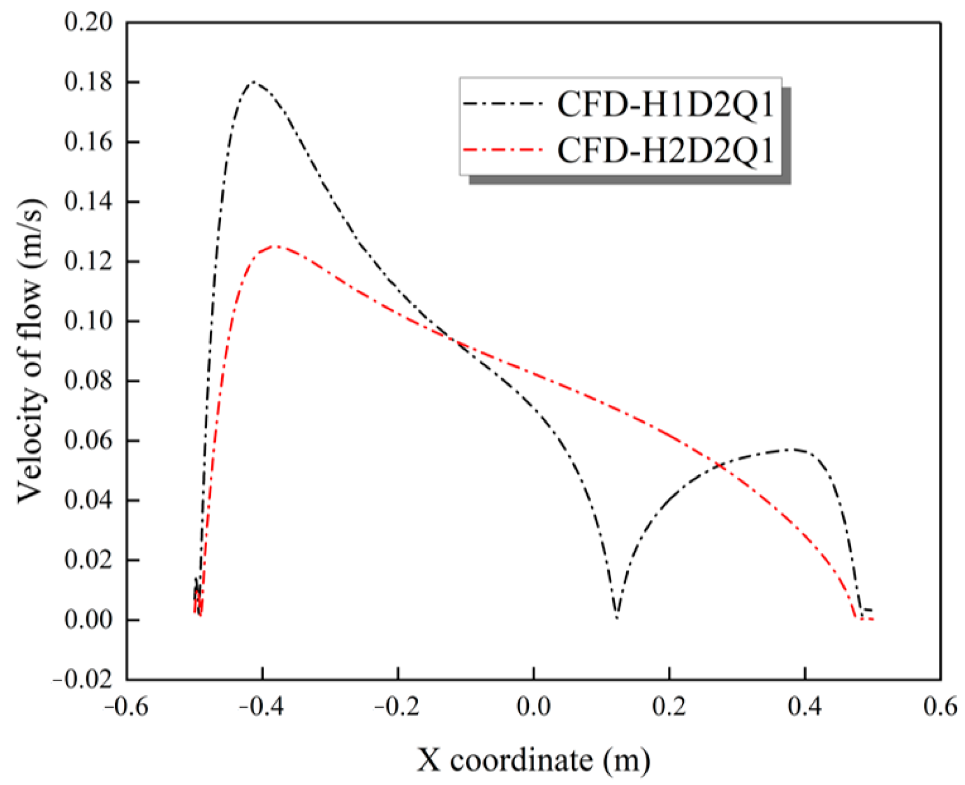
As shown in Figure 15, the position of the maximal Kolmogorov scale at the gas–liquid interface moves towards the negative direction of the z-axis as the pipe diameter decreases. In the meantime, as shown in Figure 16, the overall Kolmogorov scale near the gas–liquid interface decreases, and the renewal effect of microscopic vortices increases. Figure 17 illustrates the flow velocity distribution along line 1 of the geometric model, demonstrating that the overall flow velocity of a small jet diameter is greater than that of a large jet diameter. At this time, the renewal effect of vortex 1 and vortex 2 on the fluid at the gas–liquid interface is stronger for jets with a small diameter.
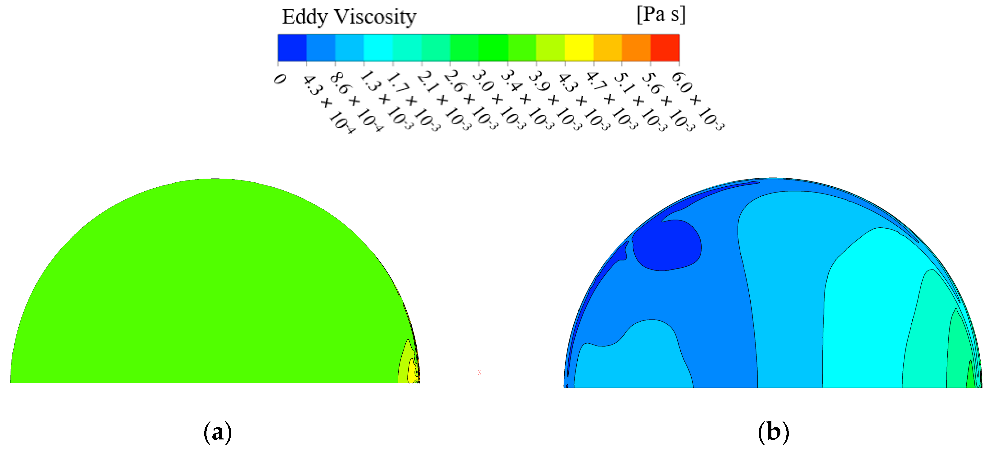
Figure 18 shows the turbulent viscosity distribution at the gas–liquid interface, and according to Equation (13), the factors causing diffusion are molecular diffusion and turbulent diffusion, and generally, turbulent diffusion is much larger than molecular diffusion, and the turbulent diffusion coefficient increases with the increase in turbulent viscosity. Therefore, it can be seen from Figure 18 that the turbulent diffusion coefficient on the gas–liquid interface in the base condition is relatively uniform, and when the jet diameter becomes smaller, the turbulent diffusion coefficient on the right side is stronger, the distribution is shifted, and the overall turbulent intensity is increased.
The fluid renewal time , as shown in Equation (24), is the time required for the fluid in the VCT to be replaced all over at the experimental flow rate.
where is the volume of the VCT, is the jet flow rate, and is the jet diameter.
According to the law of mass conservation, the mass of fluid entering the VCT per unit of time is equal to the outflow mass. Therefore, the shorter the fluid renewal time, the greater the fluid circulation per unit of time, and the stronger the renewal effect, the higher the fluid concentration at the gas–liquid interface. The jet diameter does not affect the inlet flow rate, only the jet velocity. As the jet diameter decreases, the jet velocity increases at a constant flow rate, and the jet energy becomes more concentrated. The impact of the jet on the side wall surface will be diffused in all directions along the wall, with a stronger impact and diffusion resulting from a higher flow velocity. Therefore, the impact on the gas–liquid interface is also stronger as the mass transfer coefficient increases.
Equation (22) can be written in the form expressed in terms of fluid update time , as shown in Equation (25), where and represent the jet velocity and fluid update time, respectively, of CFD-H1D2Q1 for the base case.
In summary, the jet diameter changes only the jet velocity , leading to changes in the Kolmogorov scale and macroscopic flow field structure, which affects the mass transfer process.
4.4. Effect of Jet Height on Mass Transfer Process
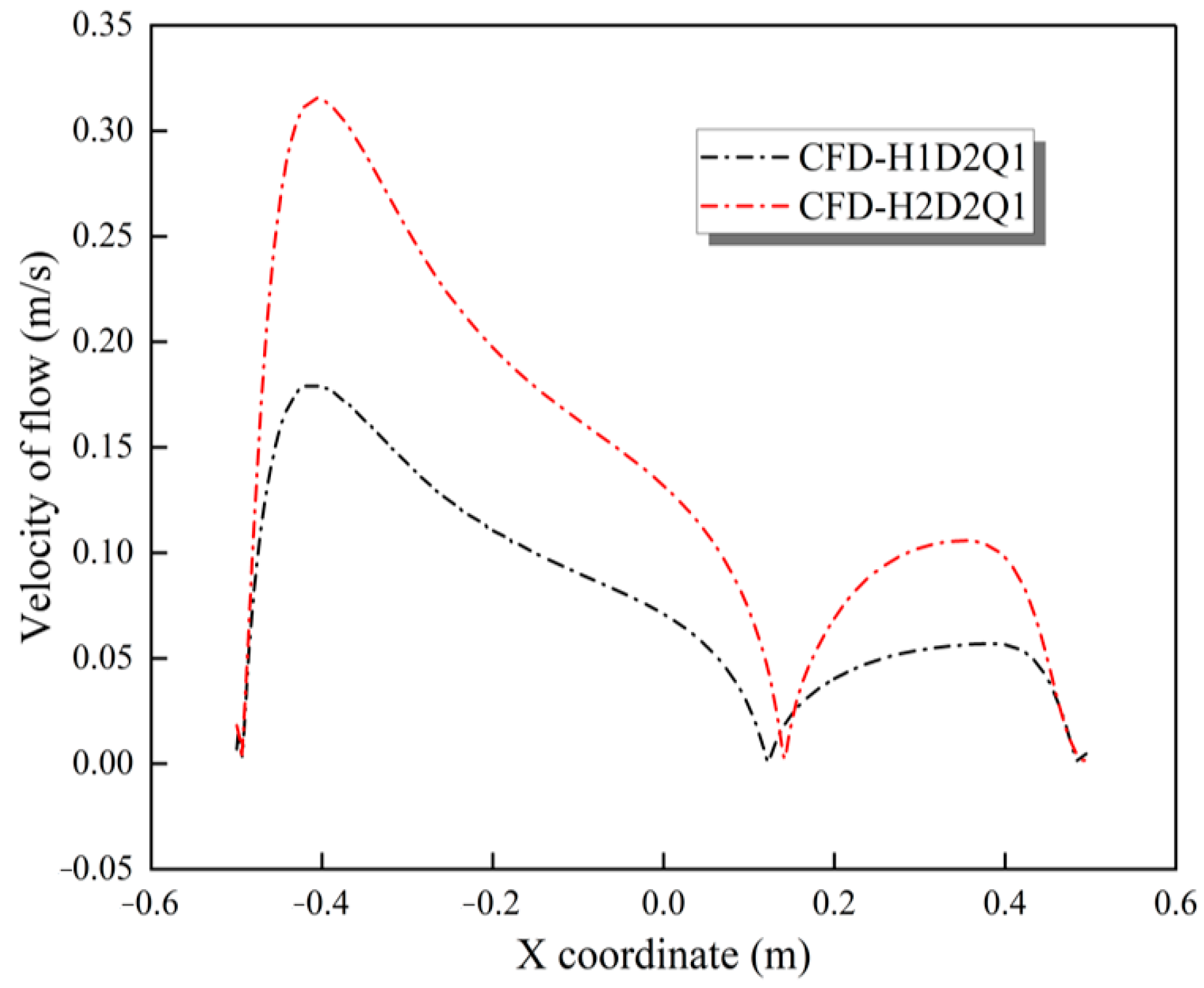
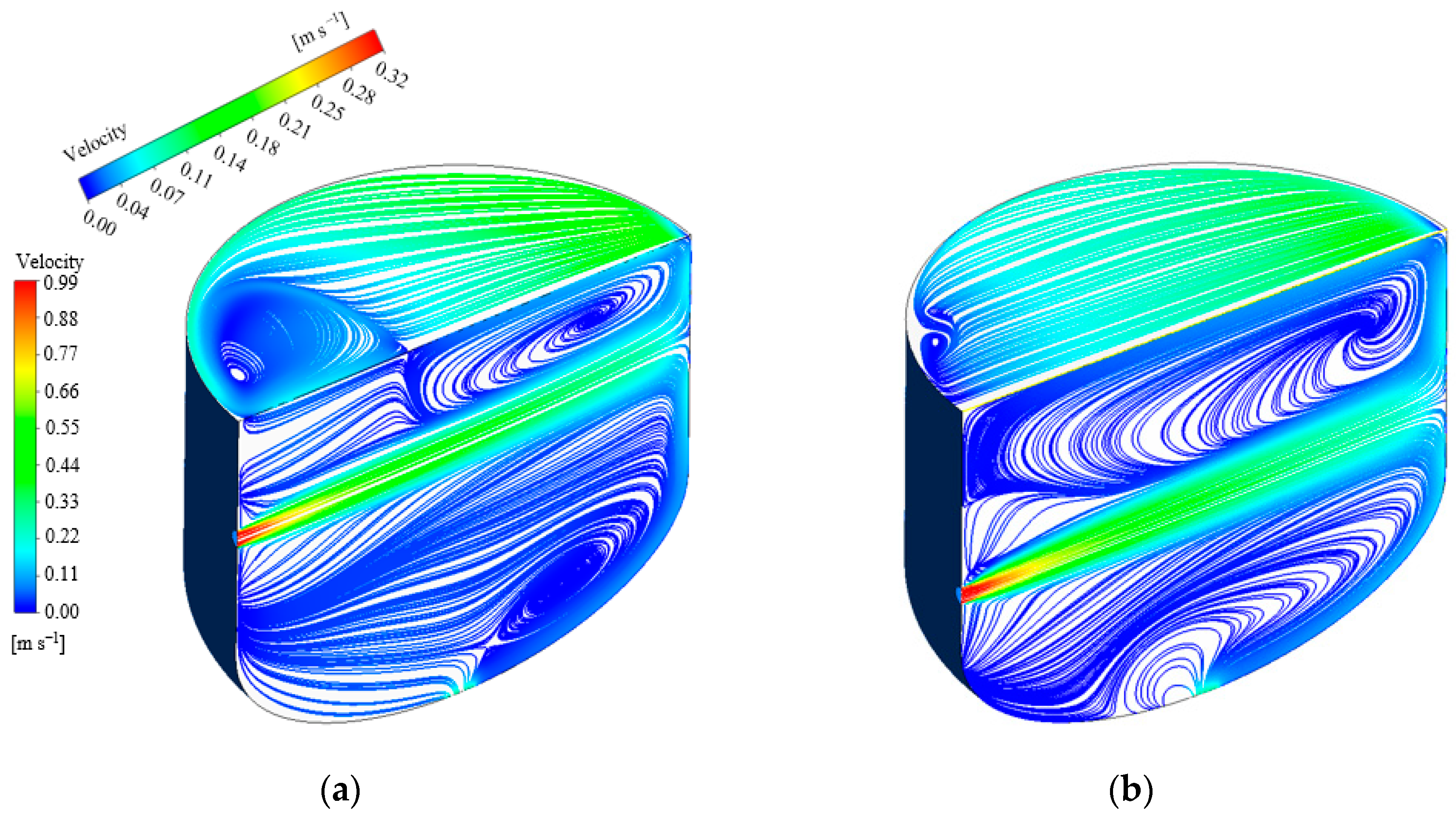
Figure 19 shows the streamline charts for different jet heights. As shown in Figure 19, as the jet inlet is shifted down, the flow of the surface jet formed by the jet impact to reach the gas–liquid interface increases, as does the loss along the jet. At the same time, the angle between the velocity vector and the x-axis at the gas–liquid interface changes from 45° to 0° after the jet inlet is shifted downward, and the reduction of the angle causes the vortex 1 above the jet inlet to be compressed, and the surface jet is less disturbed by the vortex 1. As shown in Figure 20, the surface jet flow velocity in the high-inlet case is greater than that in the low-inlet case at the distance from the jet inlet. Due to the effect of vortex 1, the surface jet decays faster in the high-inlet case and decays to a level lower than that of the low-inlet case at x = −0.16 m. After entering the vortex 2 body range, the surface jet velocity of the high-inlet condition regains its rise. With x = 0.28 m as the dividing line, the surface jet velocities of the high-inlet case and the low-inlet case are both dominant. In general, the effect of the change of jet height on the surface jet update is minimal.
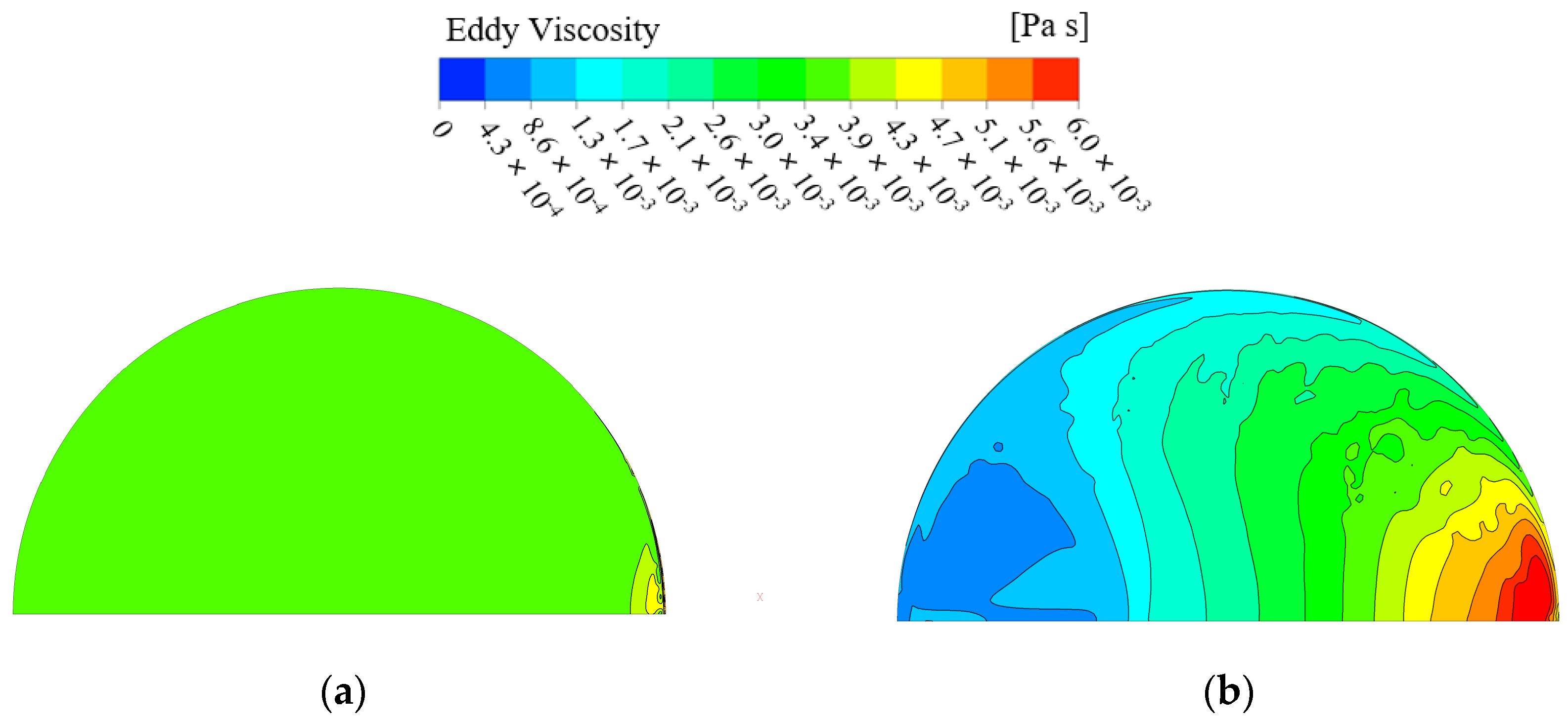
Moreover, it can be seen from Figure 21 that the turbulent viscosity at the gas–liquid interface in the base case is relatively uniform; thus, the turbulent diffusion coefficient is relatively uniform. When the jet height increases, the turbulent diffusion coefficient on the right side is stronger, the distribution is shifted, and the overall turbulence intensity decreases.
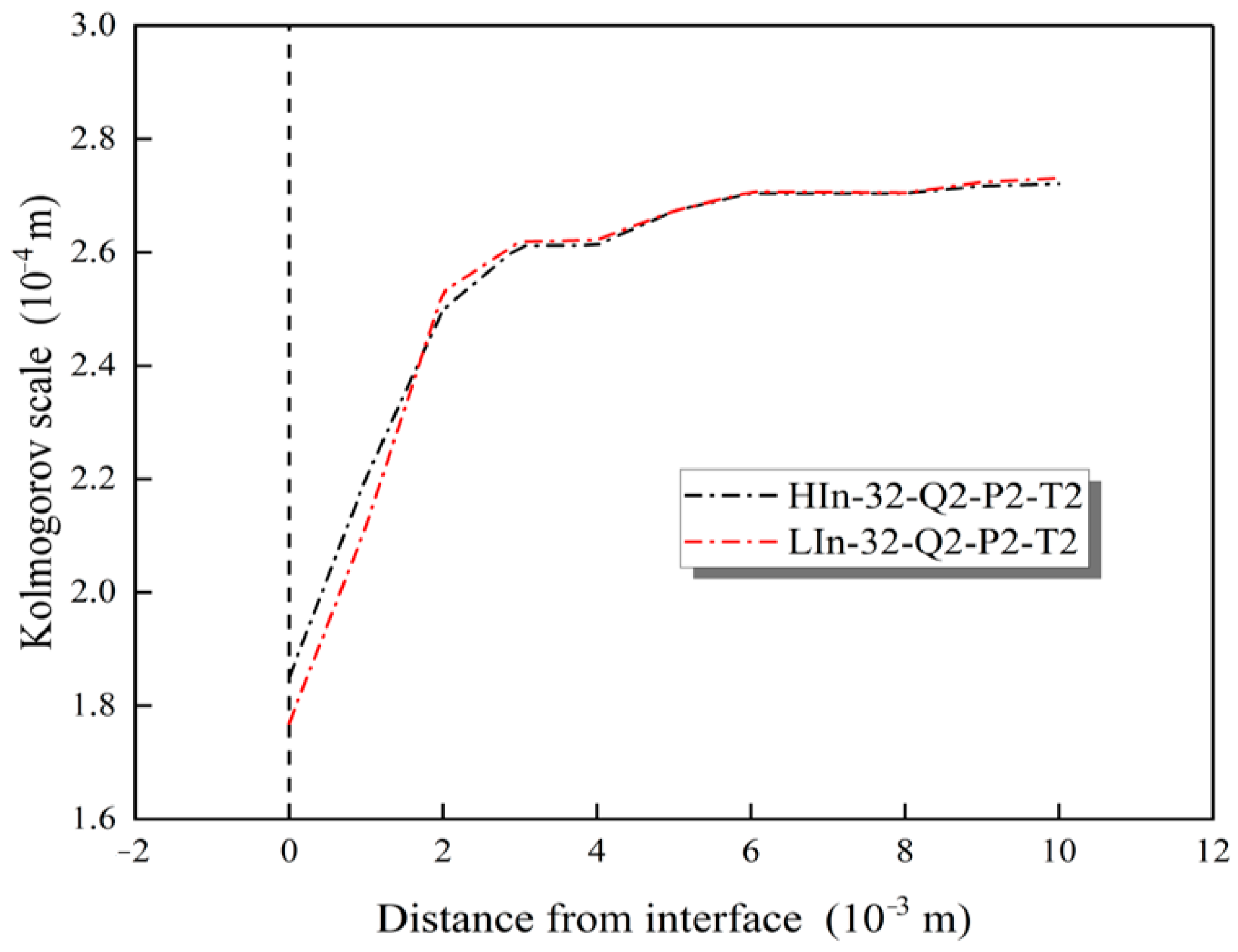
As shown in Figure 22, in addition to the structure of the macroscopic flow field, the reduction of the jet height also leads to an increase in the Kolmogorov scale at the side of the gas–liquid interface located in the negative direction of the x-axis and a decrease in the Kolmogorov scale at the side of the positive direction of the x-axis. The overall Kolmogorov scale near the gas–liquid interface, shown in Figure 23, does not change much. In conclusion, both the macroscopic flow field structure and the Kolmogorov scale distribution are influenced by the jet height, but the overall effect is small.
5. Conclusions
In this paper, the gas–liquid mass transfer near the phase interface in the VCT was investigated using a CFD model coupled with the surface divergence model. The coupled model was validated by the experiment data.
The analysis of the physical field characteristics reveals three flow field structures that dominate the entire mass transfer process. The first is the double-vortex structure above the jet inlet, which has an entrainment effect on the fluid near the gas–liquid interface. The second is the surface jet at the gas–liquid interface, which flows over the gas–liquid interface with a continuous renewal of high-concentration fluids upstream of the surface jet. The third is the vortex at the end of the jet on the symmetry surface, which displaces the high-concentration fluid at the gas–liquid interface with the low-concentration fluid at the end of the jet.
Moreover, the influence of the structural parameters of the VCT on the gas–liquid mass transfer has been studied. There are two dominant factors that affect the gas–liquid mass transfer. They are the Kolmogorov scale and the macroscopic flow field structure. With the decrease in the jet diameter, the two factors enhance the mass transfer between the gas and liquid phases together. Moreover, both the macroscopic flow field structure and the Kolmogorov scale distribution are strongly influenced by the jet height, but these two effects cancel each other. Hence, the effect of jet height on the mass transfer near the phase interface is ultimately negligible.
Author Contributions
Conceptualization, J.H. and W.L.; methodology, J.H.; software, X.C.; validation, J.H., W.L. and X.C.; formal analysis, J.H.; investigation, J.H.; data curation, X.C.; writing—original draft preparation, J.H. and W.L.; writing—review and editing, J.H.; supervision, N.W.; project administration, N.W. All authors have read and agreed to the published version of the manuscript.
Funding
This work was financially supported by Key R&D Program of Shandong Province, China (No. 2020CXGC010306).
Data Availability Statement
Not applicable.
Acknowledgments
The scientific calculations in this paper were completed on the HPC Cloud Platform of Shandong University.
Conflicts of Interest
The authors declare no conflict of interest.
References
- Chi, X.; Dong, P.; Wang, N. Numerical investigation of the fluid retention in the tank with a horizontal negatively buoyant jet. Prog. Nucl. Energy 2023, 156, 104558. [Google Scholar] [CrossRef]
- Kuschewski, M.; Kulenovic, R.; Laurien, E. Experimental setup for the investigation of fluid-structure interactions in a T-junction. Nucl. Eng. Des. 2013, 264, 223–230. [Google Scholar] [CrossRef]
- Mehassouel, A.; Derriche, R.; Bouallou, C. Kinetics study and simulation of CO2 absorption into mixed aqueous solutions of methyldiethanolamine and hexylamine. Oil Gas Sci. Technol. 2018, 73, 19. [Google Scholar] [CrossRef]
- Janzen, J.G.; Herlina, H.; Jirka, G.H.; Schulz, H.E.; Gulliver, J.S. Estimation of mass transfer velocity based on measured turbulence parameters. AIChE J. 2009, 56, 2005–2017. [Google Scholar] [CrossRef]
- Kermani, A.; Shen, L. Surface age of surface renewal in turbulent interfacial transport. Geophys. Res. Lett. 2009, 36, L10605. [Google Scholar] [CrossRef]
- Xu, Z.F.; Khoo, B.C.; Carpenter, K. Mass transfer across the turbulent gas-water interface. AIChE J. 2006, 52, 3363–3374. [Google Scholar] [CrossRef]
- Turney, D.E.; Banerjee, S. Air–water gas transfer and near-surface motions. J. Fluid Mech. 2013, 733, 588–624. [Google Scholar] [CrossRef]
- Jirka, G.H. Experiments on gas transfer at the air-water interface induced by oscillating grid turbulence. J. Fluid Mech. 2008, 594, 183–208. [Google Scholar]
- Jirka, G.H.; Herlina, H.; Niepelt, A. Gas transfer at the air-water interface: Experiments with different turbulence forcing mechanisms. Exp. Fluids 2010, 49, 319–327. [Google Scholar] [CrossRef]
- Lovatte, E.; Furieri, B.; Reis, N.; Santos, J.; Dourado, H. Large-eddy simulations of turbulent flow structures near a quiescent liquid–gas interface for gaseous compounds emissions studies. Appl. Math. Model. 2017, 42, 29–42. [Google Scholar] [CrossRef]
- Nagaosa, R.; Handler, R.A. Characteristic time scales for predicting the scalar flux at a free surface in turbulent open-channel flows. AIChE J. 2012, 58, 3867–3877. [Google Scholar] [CrossRef]
- Dani, A.; Cockx, A.; Legendre, D.; Guiraud, P. Effect of spheroid bubble interface contamination on gas-liquid mass transfer at intermediate Reynolds numbers: From DNS to Sherwood numbers. Chem. Eng. Sci. 2022, 248, 116979. [Google Scholar] [CrossRef]
- Dong, Y.H.; Lu, X.Y. Direct numerical simulation of stably and unstably stratified turbulent open channel flows. Acta Mech. 2005, 177, 115–136. [Google Scholar] [CrossRef]
- Teraoka, R.; Sugihara, Y.; Nakagawa, T.; Matsunaga, N. Numerical study on free-surface turbulence in thermally-stratified open-channel flows. Annu. J. Hydraul. Eng. 2015, 59, 583–588. [Google Scholar]
- Wissink, J.G.; Herlina, H. Effect of free-slip and no-slip boundaries on isotropic turbulence. ERCOFTAC Ser. 2020, 27, 17–23. [Google Scholar]
- Herlina, H.; Wissink, J.G. Isotropic-turbulence-induced mass transfer across a severely contaminated water surface. J. Fluid Mech. 2016, 797, 665–682. [Google Scholar] [CrossRef]
- Khakpour, H.R.; Shen, L.; Yue, D.K.P. Transport of passive scalar in turbulent shear flow under a clean or surfactant-contaminated free surface. J. Fluid Mech. 2011, 670, 527–557. [Google Scholar] [CrossRef]
- Lu, J.; Dai, H.C. Effect of submerged vegetation on solute transport in an open channel using large eddy simulation. Adv. Water Resour. 2016, 97, 87–99. [Google Scholar] [CrossRef]
- Huang, H.; Zeng, S.; Luo, C.; Long, T. Separate effect of turbulent pulsation on internal mass transfer in porous biofilms. Environ. Res. 2023, 217, 114972. [Google Scholar] [CrossRef]
- Sanjou, M.; Nezu, I.; Okamoto, T. Surface velocity divergence model of air/water interfacial gas transfer in open-channel flows. Phys. Fluids 2017, 29, 1460–1467. [Google Scholar] [CrossRef]
- Wissink, J.G.; Herlina, H. Direct numerical simulation of gas transfer across the air-water interface driven by buoyant convection. J. Fluid Mech. 2016, 787, 508–540. [Google Scholar] [CrossRef]
- Sanjou, M. Local gas transfer rate through the free surface in spatially accelerated open-channel turbulence. Phys. Fluids 2020, 32, 105103. [Google Scholar] [CrossRef]
- Liu, F.; Chen, H.; Chen, J. Numerical simulation of shock wave problems with the two-phase two-fluid model. Prog. Nucl. Energy 2020, 121, 103259. [Google Scholar] [CrossRef]
- Sosnowski, M. Evaluation of heat transfer performance of a multi-disc sorption bed dedicated for adsorption cooling technology. Energies 2019, 12, 4660. [Google Scholar] [CrossRef]
- Roache, P.J. Perspective: A method for uniform reporting of grid refinement studies. J. Fluids Eng. 1994, 116, 405–413. [Google Scholar] [CrossRef]
- Su, Q.; Wang, N.; Chi, X. An experimental study of the gas-liquid mass transfer in the volume control tank. In Proceedings of the 29th International Conference on Nuclear Engineering, Beijing, China, 8–12 August 2022. [Google Scholar]
- Xu, H.; Bodenschatz, E. Motion of inertial particles with size larger than Kolmogorov scale in turbulent flows. Phys. D Nonlinear Phenom. 2008, 237, 2095–2100. [Google Scholar] [CrossRef]
Figure 1.
RCV system diagram.

Figure 2.
Geometric model.

Figure 3.
CFD mesh.

Figure 4.
Experimental system diagram.

Figure 5.
Physical diagram of the VCT.

Figure 6.
Structure of the VCT (mm).

Figure 7.
Jet inlet (mm): (a) Inner diameter is 16 mm; (b) Inner diameter is 32 mm; (c) Inner diameter is 49 mm.
Figure 7.
Jet inlet (mm): (a) Inner diameter is 16 mm; (b) Inner diameter is 32 mm; (c) Inner diameter is 49 mm.

Figure 8.
Concentration field distribution of the VCT: (a) Symmetry; (b) Wall. (t = 1500 s).

Figure 9.
Outlet concentration and volume-averaged concentration curves of oxygen in the VCT.

Figure 10.
Streamline chart of the VCT: (a) Streamline chart of the gas–liquid interface; (b) Streamline chart of the symmetry plane. (t = 1500 s).
Figure 10.
Streamline chart of the VCT: (a) Streamline chart of the gas–liquid interface; (b) Streamline chart of the symmetry plane. (t = 1500 s).

Figure 11.
Experimental correlation equation for the dimensionless mass transfer coefficient (Sh).

Figure 12.
Dissolved oxygen concentration curves at the outlet of the VCT for different jet diameters: (a) Q1; (b) Q2.
Figure 12.
Dissolved oxygen concentration curves at the outlet of the VCT for different jet diameters: (a) Q1; (b) Q2.

Figure 13.
Dissolved oxygen concentration curves at the outlet of the VCT at different jet heights.

Figure 14.
Comparison of CFD data with EXP data.

Figure 15.
Kolmogorov scale distribution at the gas–liquid interface: (a) CFD-H1D2Q1; (b) CFD-H1D1Q1. (t = 1500 s).
Figure 15.
Kolmogorov scale distribution at the gas–liquid interface: (a) CFD-H1D2Q1; (b) CFD-H1D1Q1. (t = 1500 s).

Figure 16.
Effect of jet diameter on Kolmogorov scale.

Figure 17.
Effect of jet diameter on velocity.

Figure 18.
Turbulent viscosity distribution at the gas–liquid interface: (a) CFD-H1D2Q1; (b) CFD-H1D1Q1. (t = 1500 s).
Figure 18.
Turbulent viscosity distribution at the gas–liquid interface: (a) CFD-H1D2Q1; (b) CFD-H1D1Q1. (t = 1500 s).

Figure 19.
Effect of jet height on the streamline chart: (a) CFD-H1D2Q1; (b) CFD-H2D2Q1. (t = 1500 s; the left side is the legend of the symmetry plane, and the upper side is the legend of the division interface).
Figure 19.
Effect of jet height on the streamline chart: (a) CFD-H1D2Q1; (b) CFD-H2D2Q1. (t = 1500 s; the left side is the legend of the symmetry plane, and the upper side is the legend of the division interface).

Figure 20.
Effect of jet height on velocity.

Figure 21.
Turbulent viscosity distribution at the gas–liquid interface: (a) CFD-H1D2Q1; (b) CFD-H2D2Q1. (t = 1500 s).
Figure 21.
Turbulent viscosity distribution at the gas–liquid interface: (a) CFD-H1D2Q1; (b) CFD-H2D2Q1. (t = 1500 s).

Figure 22.
Kolmogorov scale distribution at the gas–liquid interface: (a) CFD-H1D2Q1; (b) CFD-H2D2Q1. (t=1500 s).
Figure 22.
Kolmogorov scale distribution at the gas–liquid interface: (a) CFD-H1D2Q1; (b) CFD-H2D2Q1. (t=1500 s).

Figure 23.
Effect of jet height on Kolmogorov scale.


Table 1.
Boundary condition settings.
| Location | Boundary Type |
|---|---|
| Jet inlet | Velocity-Inlet |
| Tank bottom outlet | Pressure-Outlet |
| Tank wall surface | No-Slip wall surface |
| Symmetrical surface | Symmetry boundary |
| Gas–liquid interface | Zero-shear interface |
Table 2.
Numerical simulation working conditions table.
| Number | Inlet Height (mm) | Jet Diameter (mm) | Inlet Flow Rate (m3/h) | Total Pressure (kPa) | Fluid Temperature (°C) |
|---|---|---|---|---|---|
| CFD-H1D2Q1 | 236.5 | 32 | 2.80 | 140.0 | 30.0 |
| CFD-H2D2Q1 | 361.5 | 32 | 2.80 | 140.0 | 30.0 |
| CFD-H1D1Q1 | 236.5 | 16 | 2.80 | 140.0 | 30.0 |
Table 3.
Mesh parameters and quantities values.
| N (-) | KL (10−5 m/s) | H (-) | R (-) | (-) | (-) | P (-) | (%) | GCI (%) |
|---|---|---|---|---|---|---|---|---|
| 267,412 | 1.880 | 9.83 | - | - | converged | 9.59 | 1.90 | 0.42 |
| 500,349 | 2.205 | 7.97 | 1.23 | 0.3250 | ||||
| 904,440 | 2.248 | 6.55 | 1.22 | 0.0430 |
Table 4.
Experimental working conditions table.
| Number | Inlet Height (mm) | Jet Diameter (mm) | Inlet Flow Rate (m3/h) | Total Pressure (kPa) | Fluid Temperature (°C) |
|---|---|---|---|---|---|
| EXP-H1D2Q1 | 236.5 | 32 | 2.79 | 140.6 | 29.2 |
| EXP-H1D1Q2 | 236.5 | 16 | 5.59 | 140.7 | 29.6 |
| EXP-H1D2Q2 | 236.5 | 32 | 5.60 | 139.2 | 30.5 |
| EXP-H1D3Q2 | 236.5 | 49 | 5.60 | 140.6 | 29.1 |
| EXP-H2D2Q1 | 361.5 | 32 | 2.80 | 141.0 | 29.0 |
| EXP-H1D1Q1 | 236.5 | 16 | 2.82 | 139.3 | 30.3 |
| EXP-H1D3Q1 | 236.5 | 49 | 2.78 | 141.1 | 30.0 |
Disclaimer/Publisher’s Note: The statements, opinions and data contained in all publications are solely those of the individual author(s) and contributor(s) and not of MDPI and/or the editor(s). MDPI and/or the editor(s) disclaim responsibility for any injury to people or property resulting from any ideas, methods, instructions or products referred to in the content. |
© 2023 by the authors. Licensee MDPI, Basel, Switzerland. This article is an open access article distributed under the terms and conditions of the Creative Commons Attribution (CC BY) license (https://creativecommons.org/licenses/by/4.0/).
Share and Cite
MDPI and ACS Style
Hu, J.; Li, W.; Chi, X.; Wang, N. Study on the Effect of Structural Parameters of Volume Control Tank on Gas–Liquid Mass Transfer. Energies 2023, 16, 4991. https://doi.org/10.3390/en16134991
AMA Style
Hu J, Li W, Chi X, Wang N. Study on the Effect of Structural Parameters of Volume Control Tank on Gas–Liquid Mass Transfer. Energies. 2023; 16(13):4991. https://doi.org/10.3390/en16134991
Chicago/Turabian StyleHu, Jian, Weiguang Li, Xiangyu Chi, and Naihua Wang. 2023. "Study on the Effect of Structural Parameters of Volume Control Tank on Gas–Liquid Mass Transfer" Energies 16, no. 13: 4991. https://doi.org/10.3390/en16134991
Note that from the first issue of 2016, this journal uses article numbers instead of page numbers. See further details here.