

Hybrid Machine Learning for Modeling the Relative Permeability Changes in Carbonate Reservoirs under Engineered Water Injection


Departamento de Engenharia de Minas e de Petróleo, Escola Politécnica da Universidade de São Paulo, São Paulo 05508-010, Brazil
*
Author to whom correspondence should be addressed.
Energies 2023, 16(13), 4849; https://doi.org/10.3390/en16134849
Submission received: 15 March 2023
/
Revised: 25 April 2023
/
Accepted: 8 June 2023
/
Published: 21 June 2023
(This article belongs to the Special Issue Enhanced Oil Recovery Processes Evaluation, Design and Implementation)
Abstract
:Advanced production methods utilize complex fluid iteration mechanisms to provide benefits in their implementation. However, modeling these effects with efficiency or accuracy is always a challenge. Machine Learning (ML) applications, which are fundamentally data-driven, can play a crucial role in this context. Therefore, in this study, we applied a Hybrid Machine Learning (HML) solution to predict petrophysical behaviors during Engineered Water Injection (EWI). This hybrid approach utilizes K-Means and Artificial Neural Network algorithms to predict petrophysical behaviors during EWI. In addition, we applied an optimization process to maximize the Net Present Value (NPV) of a case study, and the results demonstrate that the HML approach outperforms conventional methods by increasing oil production (7.3%) while decreasing the amount of water injected and produced (by 28% and 40%, respectively). Even when the injection price is higher, this method remains profitable. Therefore, our study highlights the potential benefits of utilizing HML solutions for predicting petrophysical behaviors during EWI. This approach can significantly improve the accuracy and efficiency of modeling advanced production methods, which may help the profitability of new and mature oil fields.
1. Introduction
Artificial Intelligence (AI) technologies are increasingly being applied in the oil and gas industry due to the challenges of handling large volumes of data [1,2]. Machine Learning, a subset of AI, has the advantage of efficiently processing large amounts of data and providing reliable solutions to various problems. According to [2], the number of papers on Machine Learning has been growing exponentially in recent years. Additionally, the current digital transformation acts as a catalyst for the widespread usage of these techniques [3].
Reservoir modeling and simulation require a numerical approach based on physical laws, such as mass conservation, thermodynamics, hydraulic diffusivity, etc. Although these tools are considered reliable, their results only estimate the actual measured data. Some physical phenomena have nonlinear behavior, making them complex to model. On the other hand, an alternative approach based on the relationship between the data is more advantageous in some applications, such as reservoir petrophysical behaviors [4,5,6].
Moreover, including physicochemical interactions in the simulation process, such as Enhanced Oil Recovery (EOR) injections, makes numerical estimations even more challenging. In this case, using laboratory data in the numerical model is an alternative, but this ties the solution to specific tools, limiting reproducibility to the process of generating laboratory data [7]. The EOR Engineered Water Injection (EWI) technique, which controls the salinity of the injected water to increase the volume of recovered oil, is an example of injection with a complex geochemical background [8]. This ionic control achieves polar iterations with the rock, altering its natural wettability properties and facilitating fluid permeability [9,10,11].
The geochemical behavior that occurs with injection adds more complexity to its numerical solution. Understanding these limitations, we proposed an approach through a hybrid ML solution that can learn the relationship between the variables of relative permeability, salinity (formation and injection), and mineralogy, becoming able to incorporate the changes of Kr related to the injection method.
To simplify the modeling of Engineered Water Injection, we implemented a solution with two complementary Machine Learning tools (K-Means and Artificial Neural Networks) to establish a relationship among salinity, relative permeability, and mineralogical content. Thus, we have a reliable approach with ML to reproduce the production simulation such as with conventional geochemical modeling. In this case, we initially used a clustering method to classify the original relative permeability (Kr), and subsequently, with a given injection salinity, predicted a new Kr curve. The use of these two specific ML tools defines the approach as Hybrid Machine Learning (HML).
Finally, we tested the quality of the EWI modeling pipeline with HML in an iterative optimization process. Thus, we selected a benchmark, Unisim-II, applying two injection processes: (i) with common water and (ii) with engineered water. Using the economic scenario proposed in the benchmark, we maximized the NPV with 30 years of production in both cases, increasing only the cost of the engineered water by 35%. In these tests, EWI had the highest profit increase (approximately 39%), compared to the previous injection. This performance is attributed to a 7.3% increase in oil recovery, as well as reduction in water injection volume (by 28.5%) and water production (by 40%).
2. Materials and Methods
2.1. Data Collection
The construction of the database involved using 30 templates obtained from the CMG collection, primarily designed for training and learning purposes, and are based on the well-established SPE Solution Problems benchmark problems in the industry. Each template underwent 50 simulations following a geochemical modeling approach [12]. To increase the complexity of the simulations and account for the effects of other variables, we randomly varied the salinity of formation water and the mineralogy percentages. This approach allowed us to generate a final dataset comprising 1500 simulation samples with a broad range of formation water compositions and mineralogy conditions while preserving the model characteristics for adequate generalization of scenarios during the training stage. The synthetic data generation strategy through simulation took approximately one month to complete. Finally, the dataset was ready for the KrModule, which produced the target variables for the next steps in its pipeline.
2.2. KrModule Procedure
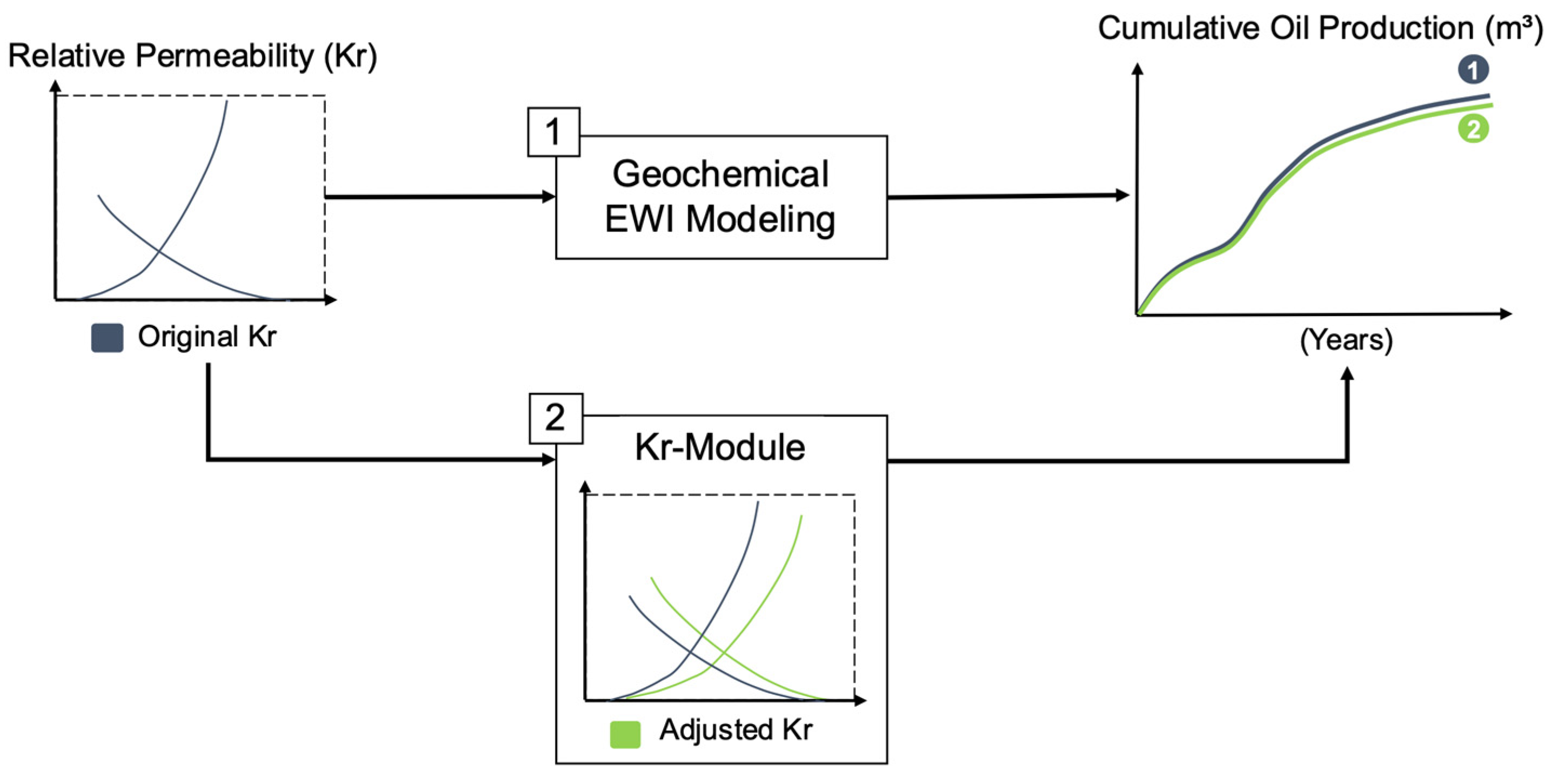
After simulating the synthetic cases, we utilized the KrModule algorithm to obtain the updated relative permeability. This algorithm works by iteratively adjusting the Kr of a model with conventional waterflooding until it generates results comparable to the corresponding EWI case (as shown in Figure 1). The KrModule is a solution developed by [12] that has been adapted for this study. In our implementation, we retained the geochemical configuration proposed by the original author, which includes the configuration for relative permeability reduction and interpolation, as well as the aqueous and mineral reactions. However, in this study, we introduced random variations in the mineral percentages and formation water content for each simulation case, which made it possible to incorporate this information into the training dataset. In comparison with the study presented in reference [12], we also made modifications to the optimizer applied in the KrModule, aiming for improved convergence of results. Thereby, we replaced the Genetic Algorithm (GA) with a Particle Swarm Optimization (PSO) algorithm, which is used to minimize the error between the production curves.
The Particle Swarm Optimization (PSO) method was employed to enhance a set of candidates or particles that move in an exploratory space through velocity and position adjustments. At each iteration, all particles are adjusted by moving toward the direction of the current best case. Once the module application was complete, we generated the new relative permeability, which reflected the effects of EWI in the simulation. Therefore, we structured the dataset as follows:
Input:
- Kr original;
- Injection salinity concentration;
- Formation salinity concentration;
- Mineralogy.
Output:
- Kr adjusted.
In our dataset of relative permeability curves for multiple samples, we observed that the water salinity and mineral content were repeatedly recorded for each data point on the curve. This led to a large dataset, which can cause training issues such as overfitting. To mitigate this problem, we transformed the actual relative permeability curves into the Brooks–Corey [13] equation parameters (Equations (1) and (2)), which provided a concise representation of the curves and synthesized all information from each sample into a single row. This transformation eliminated the repeated data, which improved the model training performance.
Kro = krocw × ((1 − Sw − Sor)/(1 − Scw − Sor))no
Krw = krwor × ((Sw − Swcrit)/(1 − Swcrit − Sor))nw
2.3. Hybrid Machine Learning Method
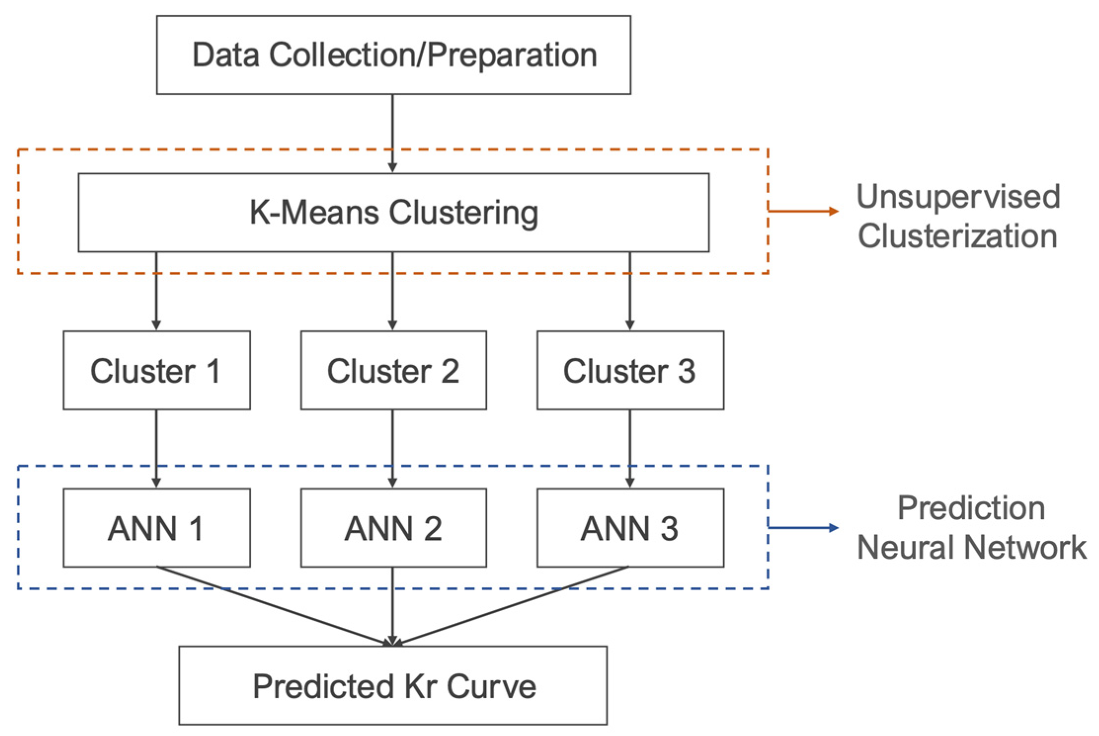
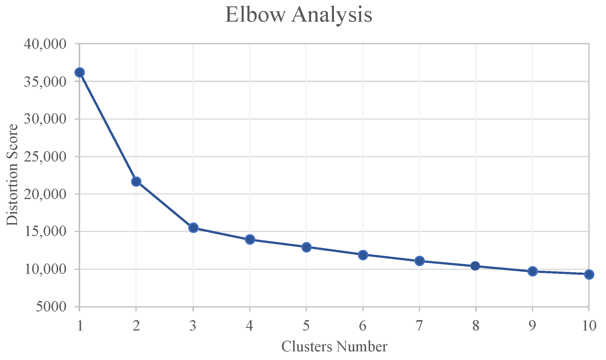
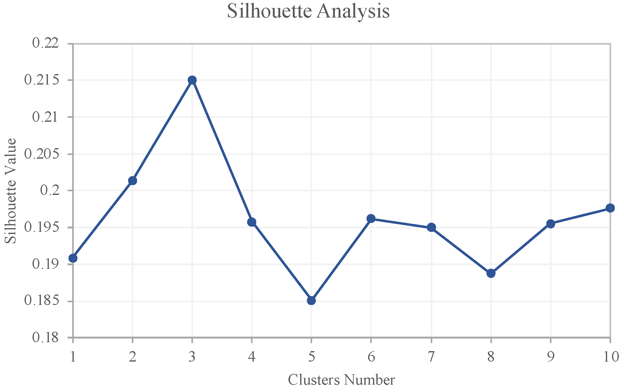
The central characteristic of the HML method involves utilizing two distinct ML algorithms. In the first stage, an unsupervised clustering process is employed, utilizing the K-Means algorithm from the Scikit-learn framework. The K-Means method groups data sets based on their similarity patterns. It is noteworthy that this algorithm does not require output labels, relying solely on the training process to identify those connections. In this stage, we conducted an elbow and silhouette analysis to determine the optimal number of clusters. The analysis results indicated that three clusters were the ideal number, which also corresponded to the number of wettability types. The other hyperparameters were set by default. Only Kr original was used as input data, thereby focusing this clustering process on the three possible groups based on input Kr.
Next, the entire data frame is divided into three parts based on the labels assigned in the clustering phase. For this stage, we opted for using Multi-Layer Perceptron (MLP) Artificial Neural Networks (ANNs) from Scikit-learn, allowing for performance comparisons with the solution proposed by [12]. Three ANNs were trained, each using one of the three corresponding new datasets (as illustrated in Figure 2). The ANN architecture consists of multiple layers of interconnected nodes (neurons). The input layer receives the data, and the output layer produces the network’s output. Between those layers, there are one or more hidden layers that perform mathematical transformations on the data. During the training process, the network’s weights are adjusted based on the difference between the actual and expected outputs, minimizing its error [13,14].
Before training the ANNs, the data set undergoes a standardization process. We used a mathematical transformation called Standard Scaler, which aims to center the data’s mean at zero and normalize the standard deviation. This helps to address the issue of data sets with vastly different feature scales, which can cause variables with high variance to overlap with the Objective Function during training, resulting in poor training performance. Equation (3) below summarizes the transformation process:
Z = (X − μ)/σ
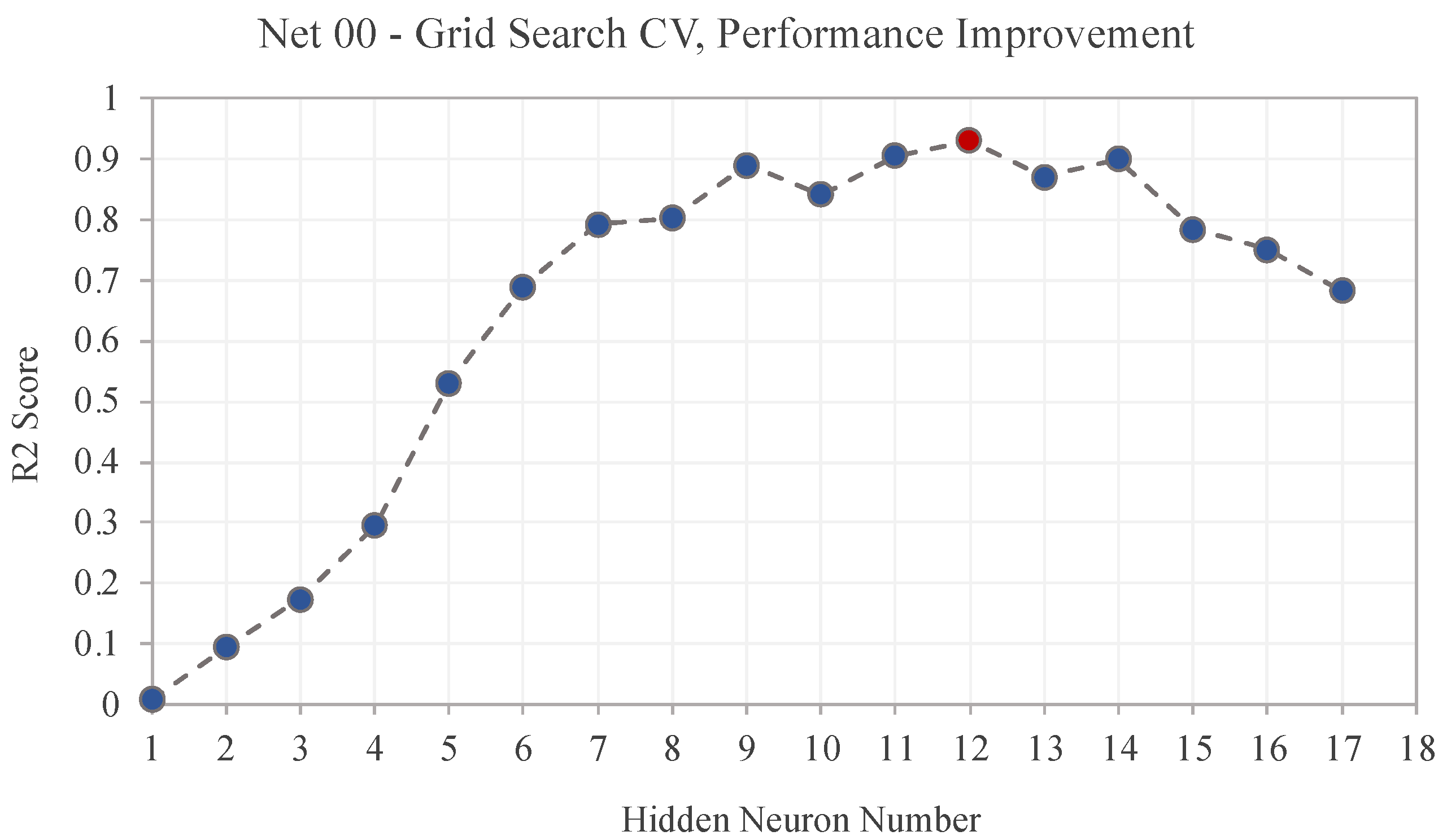
The hyperparameters of the neural networks were adjusted to enhance validation outcomes. We employed a model selection technique called Grid Search Cross Validation that systematically evaluated different combinations of ANN configurations and computed a score for each one. This enabled us to rank the results based on their predictive performance, as measured by the Normalized Mean Squared Error (NMSE) and R2 metrics. Finally, we selected the best configuration for each ANN.
The configuration and training of the K-Means model and the neural networks were completed. Then, the HML was ready to be engaged in the case study optimization process.
2.4. EWI and Water Optimization
The optimization process employed in this study aimed to maximize the NPV. To facilitate comparative analysis, we conducted two optimization runs—one using common water, and the other using EWI. To calculate the NPV, we adapted the economic scenario from the case study. The variables optimized were the well parameters: (i) flow rate and (ii) pressure. However, in the case of EWI, we included (iii) salinity concentrations of the injected water as an additional variable. Therefore, we had:
- Production rate;
- Production pressure;
- Injection rate;
- Injection pressure;
- Salinity concentrations (Na, Cl, SO4, Ca, and Mg), just in the EWI scenario.
The Particle Swarm Optimization (PSO) solution was chosen considering its simple implementation, fast convergence, and the fact that it is ideal for continuous space formulation problems. It is also a metaheuristic method, which avoids premature convergence to local minima.
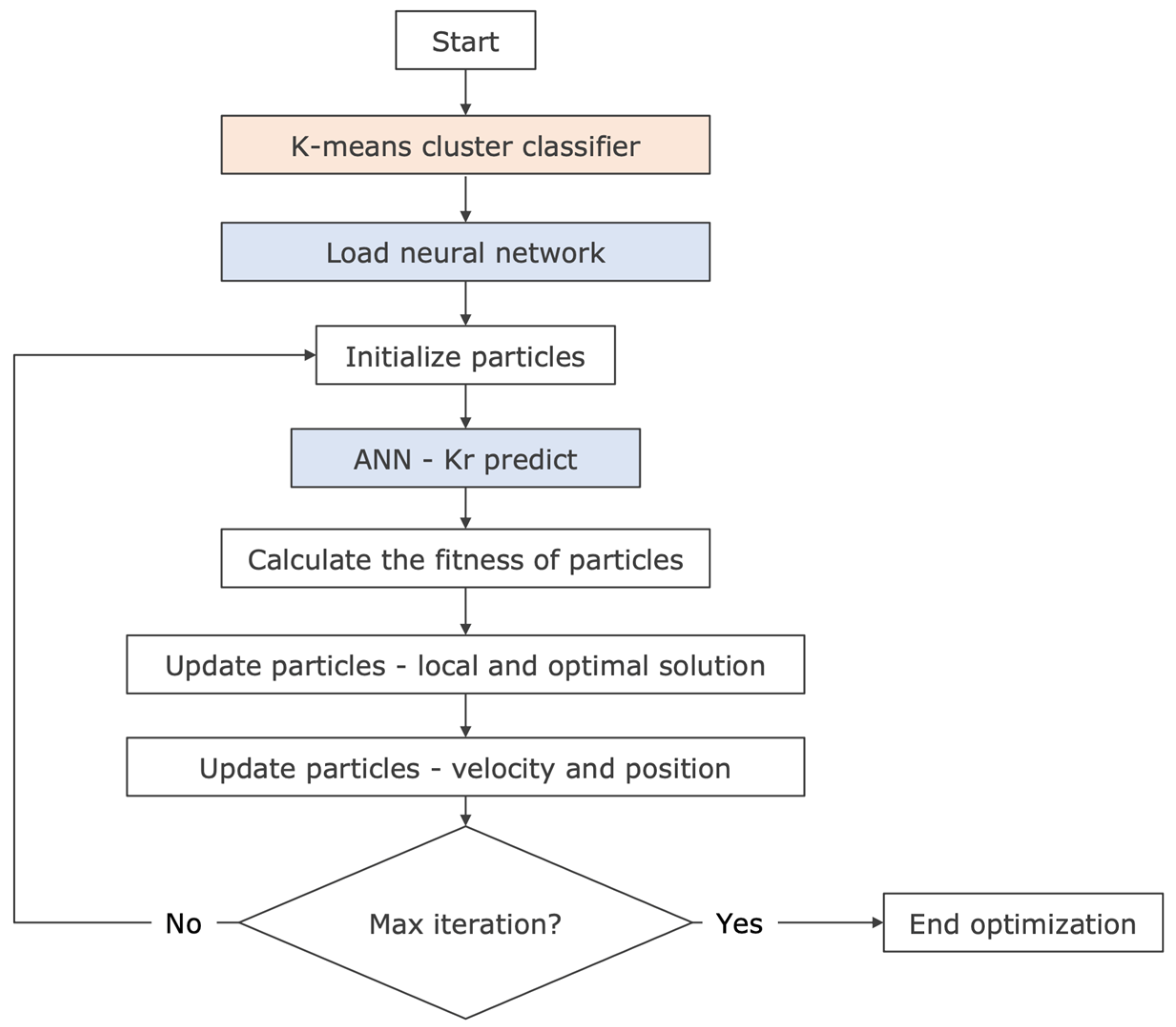
For the EWI scenario, we combined HML with optimization, which was performed in two steps. First, the K-Means model identified the original relative permeability group (or label). Then, the neural network corresponding to the group was loaded. The neural network used the salinity set at each iteration with the original Kr to predict the new curve (Figure 3).
2.5. Case Study
2.5.1. UNISIM-II Benchmark
For this project, we selected a benchmark based on a field in the Brazilian Pre-Salt. We chose the Unisim-II model, which was developed by the Unisim research group at Unicamp [15]. This case study’s structure combines data from the Ghawar and Tupi fields, which has dimensions of 5000 × 5000 × 150 m, with 16 faults and a Super-K zone [16].
The production system defined in this model provides operating ranges for the injectors and producers, and these operational limits were used in the optimization phase (Table 1).
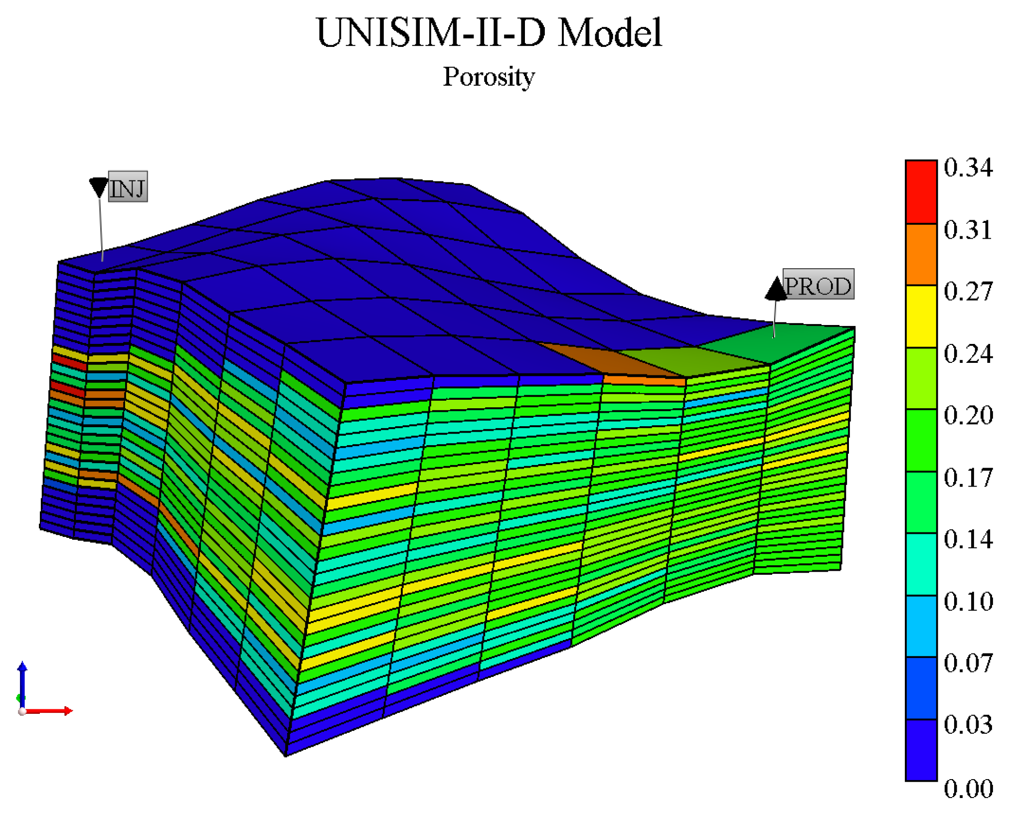
To improve the performance, we utilized a simplified version of Unisim-II, which was also used by [12]. This portion of the model comprises a representative field location with dimensions of 6 × 6 × 30 cells (Figure 4). The well configuration follows [12] and includes producer and injector wells placed in opposite corners of the model (one quarter of a five-spot pattern). Additionally, we adapted the economic scenario to match the proportions of the benchmark cut fraction, as shown in Table 2.
For the advanced injection with engineered water, we assumed a saline composition of the formation and its mineralogy. The benchmark was based in two carbonate reservoirs in which the mineralogy was 50% calcite and 50% dolomite, the most abundant minerals in this type of rock. For the ionic configuration of the formation water, we decided on 35,000 ppm of NaCl, 200 ppm of sulfate (SO42−) and magnesium (Mg2+), and 1000 ppm of calcium (Ca2+). The benchmark does not have these available data, so we defined these variables to proceed with the study.
2.5.2. KrModule PSO Parameters
The KrModule uses Particle Swarm Optimization (PSO) to adjust relative permeability with an Objective Function (OF) to reduce error between oil and water production curves. Each sample is the model with the geochemical modeling simulated. By comparing the original results, the optimizer changes in relative permeability to achieve the minimum OF. This optimizer was set as shown in Table 3.
For the constriction coefficient calculation, Equation (4) is shown below:
chi = 2 × K/|2 − (φ1 + φ2) − ((φ1 + φ2)2 − 4 × (φ1 + φ2))1/2|
2.5.3. Hybrid Machine Learning Parameters
The present study employed two Machine Learning models, each with specific hyperparameters. The K-Means model was implemented with the following settings in the pipeline:
- Number of clusters: 3;
- Method for initialization: random;
- K-Means algorithm: Lloyd.
The cluster number was determined through elbow and silhouette analyses. We employed a random state initialization method to introduce some level of randomness during the training process. For the K-Means algorithm, we selected Lloyd based on the package documentation, which indicates it is a more suitable algorithm for poorly defined clusters. We conducted preliminary tests to evaluate the impact of modifying the default parameters but found that such modifications did not significantly influence the clustering outcome. Then, the remaining parameters were set to their default values from the Scikit-learn package.
The ANN application differed in that the models were optimized using the Grid Search Cross-Validation (CV) method. The following parameters were used to configure the ANN models:
- Hidden layer size: 5 to 25;
- Activation function: logistic, tanh;
- Solver: lbfgs, sgd, adam;
- Learning rate: constant, invscaling, adaptive;
- Random state: 42.
All parameters had more than one option for tuning, and multiple combinations were explored to obtain the best configuration. For the hidden layer size, we followed the structure provided by [12], using a single layer with 10 to 25 neurons. Two activation functions were tested: the logistic sigmoid, one of the most common and computationally efficient activation functions, and the hyperbolic tangent, a nonlinear function capable of processing complex input–output relationships.
To explore the solvers and learning rate parameters, we tested all available options in the multi-layer perceptron model from Scikit-learn. To ensure that all ANNs were trained using the same deterministic randomness in the weights and bias, we set the random state to 42. All other settings for the ANN, except for those specified in the parameter list, were maintained at their default values for this application.
3. Results and Discussion
3.1. K-Means Clusterization Results
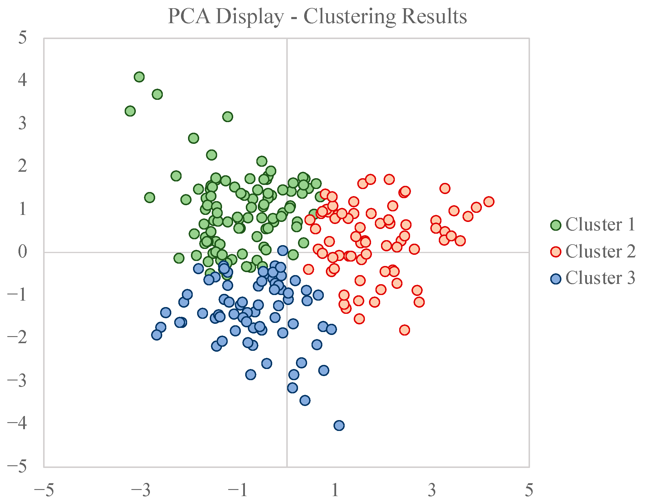
Initially, we classified the relative permeability into three groups using K-Means. Next, we utilized a dimensionality reduction method called Principal Component Analysis (PCA) to simplify the feature set. This statistical technique converts the original variables into a new set while maintaining the original variation as much as possible. We applied the reduction from eight to three components—one being the cluster labels. Thus, this allowed us to create a 2D visualization to display the data distribution by each cluster (Figure 5).
The optimal number of clusters was determined to be three using the elbow method and the silhouette analysis, as shown in Figure 6 and Figure 7. The elbow method helps to identify the ideal number of clusters by plotting the distortion values against the number of clusters. The “elbow” point is where the curvature of the plot changes direction, in other words, the optimal value. This approach aims to strike a balance between capturing the data’s variability with enough clusters without overfitting or having too many clusters with little information. On the other hand, the silhouette analysis calculates how similar each data point is to its cluster compared to others, with a score range of −1 to 1, where a higher score indicates a better match to its cluster. The optimum cluster size is the maximum silhouette value, which in this case also corresponded to three clusters (Figure 7).
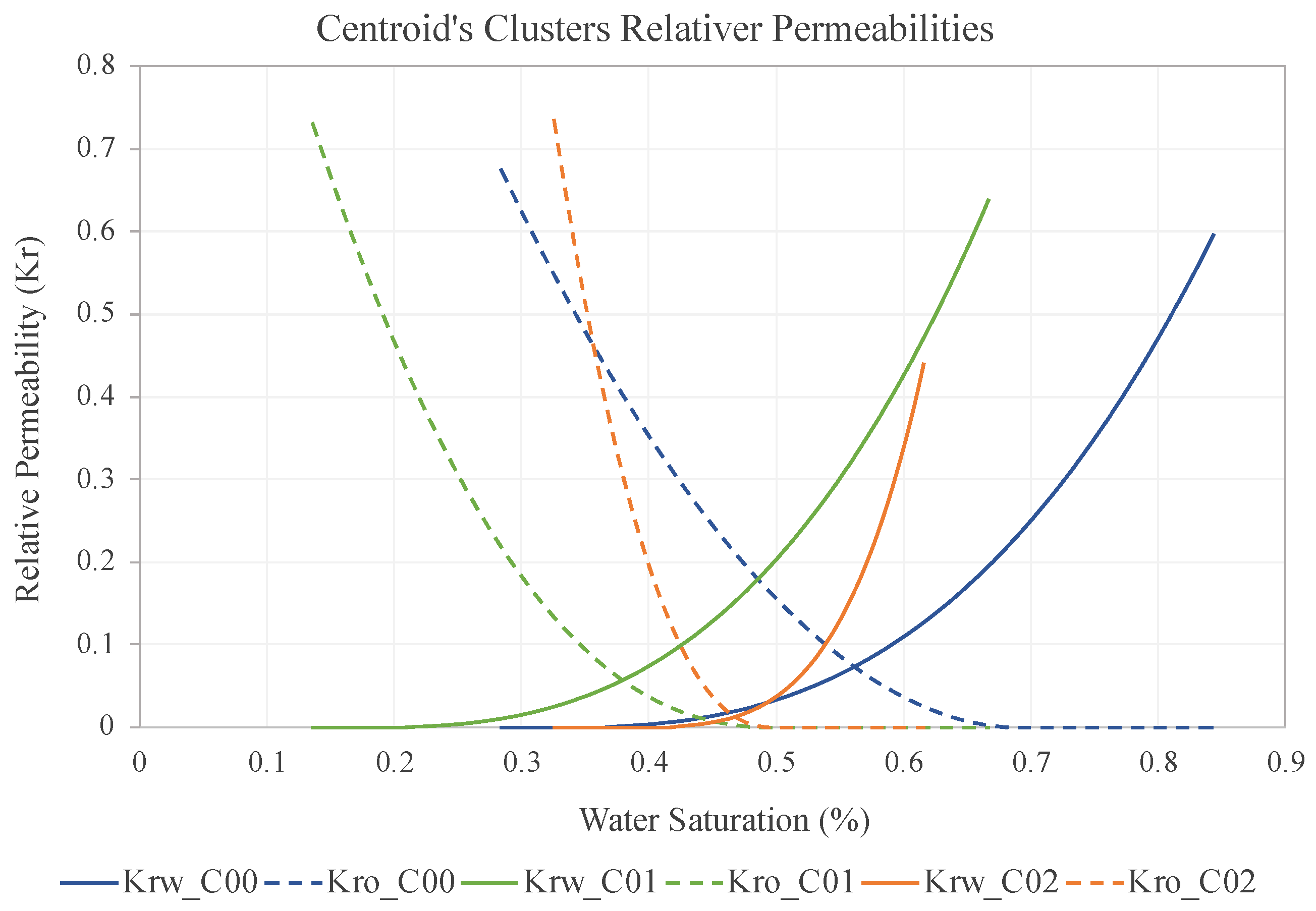
After analyzing the silhouette plot, we observed that the maximum score was 0.22, which corresponded to a cluster number of three. This result supported the selection of three clusters for the classification stage. However, the plot also indicated that the clusters were not well defined, indicating that the data points within each cluster were not very similar. Although the maximum silhouette value was below the commonly accepted threshold of 0.5 for a well-defined cluster, the data could still be grouped based on their similarities, even if they did not fit perfectly into distinct clusters. To better understand the characteristics of each cluster, we compared their centroids, which represent the overall attributes of all data points within the cluster (Figure 8).
We note here characteristics that we sought to segment at the beginning of the clustering process. The choice of three clusters in this step was not random. We used quantities of options for qualitative types of wettability, oil-wet, water-wet, and intermediate-wet, following other applications that define wettability analysis by the relative permeability curve shapes [17,18].
The features that define different wettability according to [17] method were grouped by the algorithm independently, and we can observe them through clustering centroids. Cluster 00 (in blue) has the most water-wet characteristics, with the intersection point of the Kr curves greater than 0.5 of Sw (second Craig’s rule), lower residual oil saturation (approximately 0.67 Sw), and an oil permeability curve with a lower angulation level, indicating a slower reduction in oil permeability as Sw increases. Cluster 01 (in green) has a residual oil saturation (Sor) below 0.5 Sw, a Kr–Oil curve with a large slope, and the beginning of water mobility already at low saturation (Sw at 0.25). The intermediate class is represented by cluster 02, which has characteristics between the two cases, but with the Kr–Oil starting point higher than Kr–Water, and both curves have the highest slopes.
3.2. Neural Network Results
We trained the neural network using the cross-validation method, splitting the data into 70% for training, 15% for testing, and 15% for validation. We followed the common practice in Machine Learning that recommends allocating a larger proportion (between 60–80) of data for training than for testing and validation. Therefore, we selected this proportion arbitrarily for further steps. The hyperparameters were obtained through grid search exploration, as shown in Table 4. Although the optimal network configurations did not show significant differences, their application improved the performance of predictions in all cases (Figure 9). This systematic testing of neural network configurations ensures the reliability of their performance. On the other hand, in their validation process, [12] tested two learning algorithms with a smaller range of neurons in the hidden layer, resulting in a narrower exploration of hyperparameter adjustments.
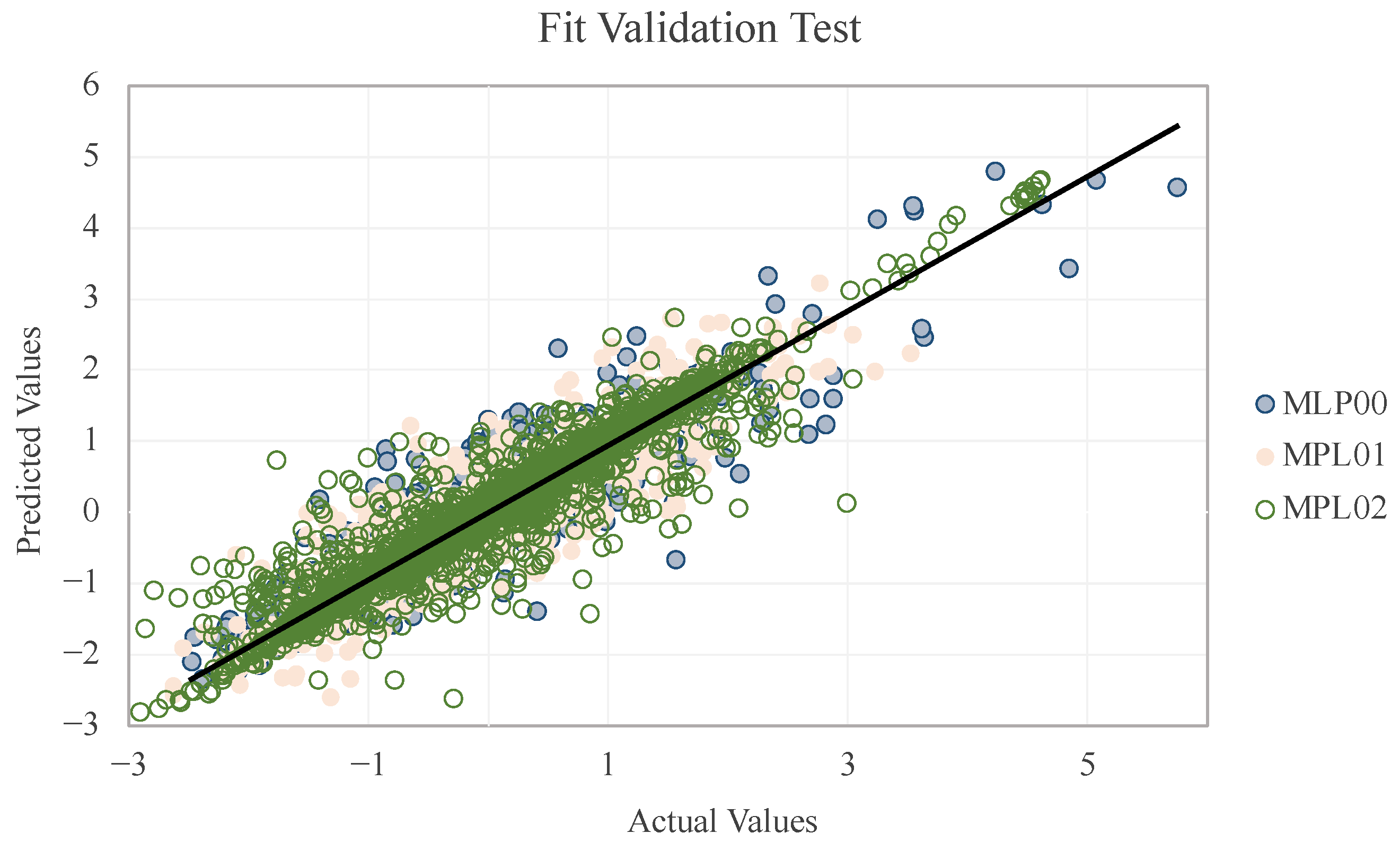
Next, using the validation fraction of the data, we compared the actual values with the predicted ones. With a cross-plot (Figure 10), it is possible to observe the distribution of the three cases approaching the expected diagonal linear regression. We confirmed the predictions via the R2 score between the actual and forecast values, which were 0.929, 0.872, and 0.897.
After optimizing the network settings, we applied the normalized root mean squared error to determine the amount of error in the prediction outcome. The resulting errors are presented below:
- Net00: 0.02940;
- Net01: 0.03627;
- Net02: 0.05106.
It is worth noting that all the errors obtained can be considered low for this prediction scenario. The predicted parameter of interest, relative permeability, ranges from 0 to 1. Therefore, even the highest error of 0.051 in the permeability value can still be considered reasonable. These results combined with the R2 results suggest that the optimized network settings provided good performance for predicting relative permeability. However, it is important to note that the results should be evaluated within the context of the specific problem being addressed.
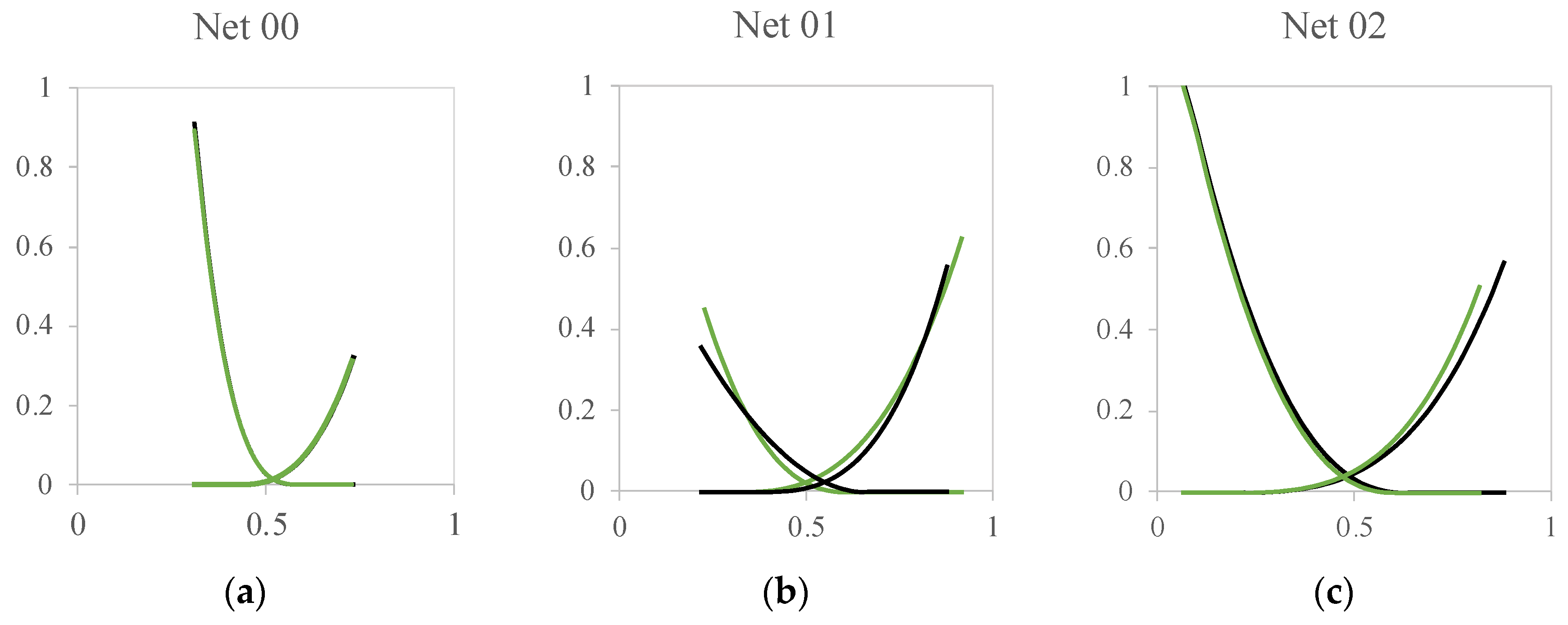
We also selected three random Kr cases from the validation to compare the shape of the forecasted curves by the networks and evaluate their quality (Figure 11).
The plots confirm that the neural network with the highest R2 score provides an accurate fit to the curves. Nevertheless, the other networks also exhibit good results in terms of curve shape. Thus, the reliability of the neural network application can be confirmed based on these results. While the R2 score of the Machine learning approach conducted by [12] is higher in absolute values (above 90%), the current approach considers more training variables, which enriches the behavior of Kr that can be predicted by the neural network. Moreover, we utilized the HML approach to train the networks with each cluster’s data, resulting in an improvement in neural network performance. By using K-Means to classify these patterns, we were able to enhance the final forecasting ability.
3.3. Optimizations
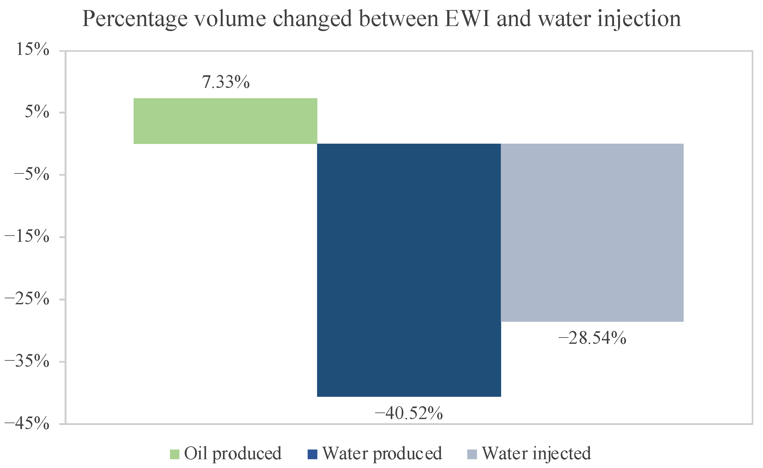
The study comprises two optimization processes: (i) Unisim-II 6 × 6 with conventional water injection and (ii) Unisim-II 6 × 6 with EWI. However, for the EOR case, we augmented the cost of injected water by 25%. In the optimization with conventional water, the best outcome yielded an NPV of MM USD 18.21 for a 30-year production period, with an oil recovery factor of 38%. Notably, the volume of water produced was six times greater than that of oil (Table 5). Although the EWI case did not result in a significant improvement in oil recovery, it led to a substantial reduction in both production and water injection volumes (by 28.5% and 40.5%, respectively) as shown in Figure 12. These changes resulted in a 45.3% increase in the final NPV result with the advanced method.
The optimized wells’ variables in the two cases showed a convergence (Table 6). The injection flow rate for the common water case was lower to control the high injection volume/production of water.
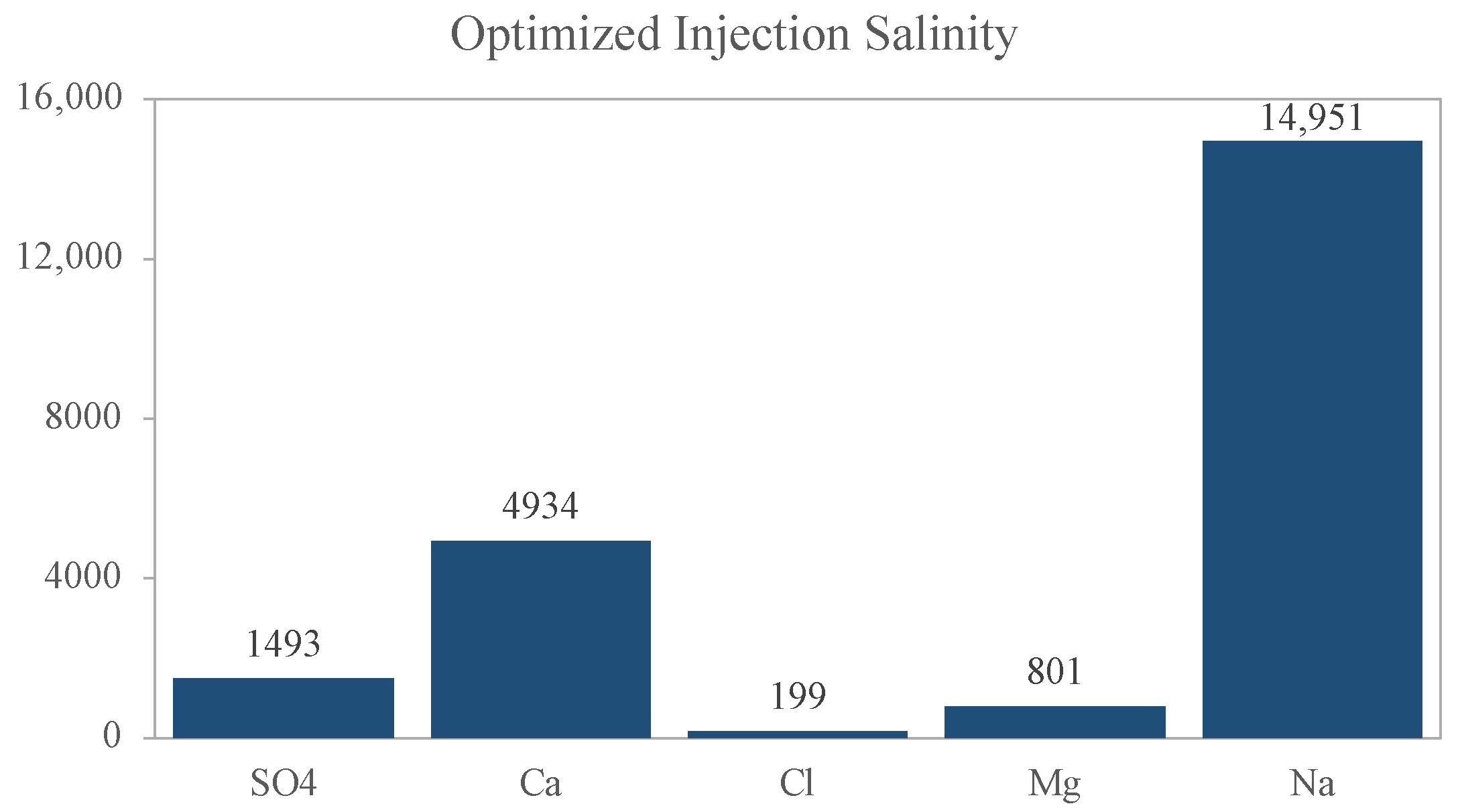
The optimum salt solution had 22,575 ppm in total, with more than half composed of sodium, as we can see in Figure 13. The sulfate concentration was increased compared to the standard saline solution. This ion is relevant for promoting the geochemical iterations of wettability reversal, so this increase in concentration was expected for the final Kr adjustment to go to a higher water wettability condition.
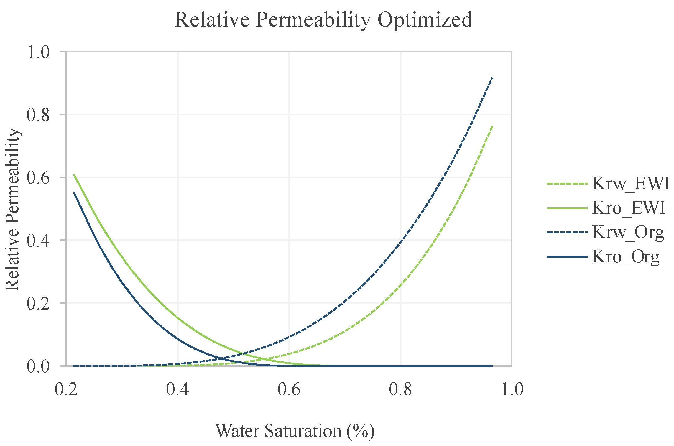
Therefore, we plotted the optimized Kr curve with the salinities compared to the original (Figure 14). Here, we see that the optimized result (green) had the Kro curve above the original case, increasing this permeability. Another important aspect is the reduction of the residual oil saturation, from 0.45 in the original case to 0.33 in the optimized case. The water condition is also changed, reducing Krw during all points of its saturation. Despite the significant changes, the new relative permeability still preserves characteristics of its base-case shape (Kr Original). However, the analyses validate the changes for increased water wettability. The Kr result of optimization performed by [12] did not preserve as many features of the same original case, caused by the smaller number of features that the model of [12] used for training. The added features decreased the change in Kr shape; it makes sense that EWI performs simple salinity changes to promote these changes.
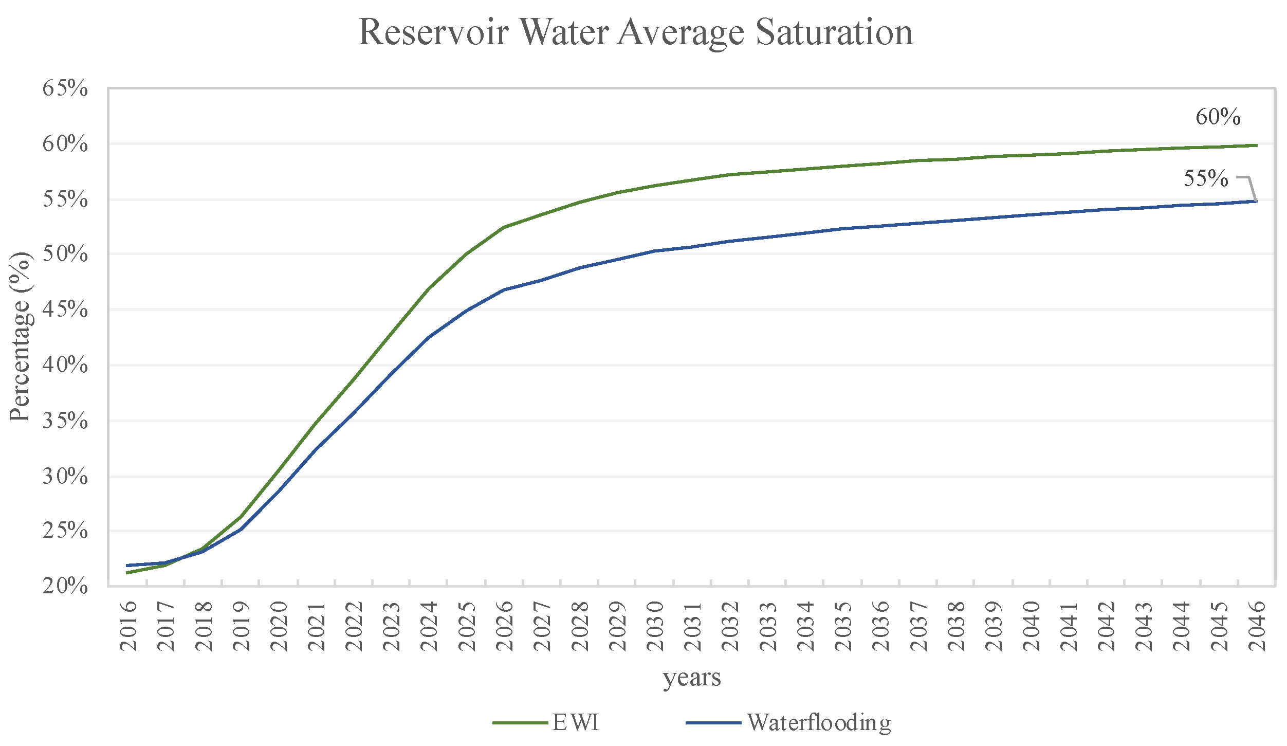
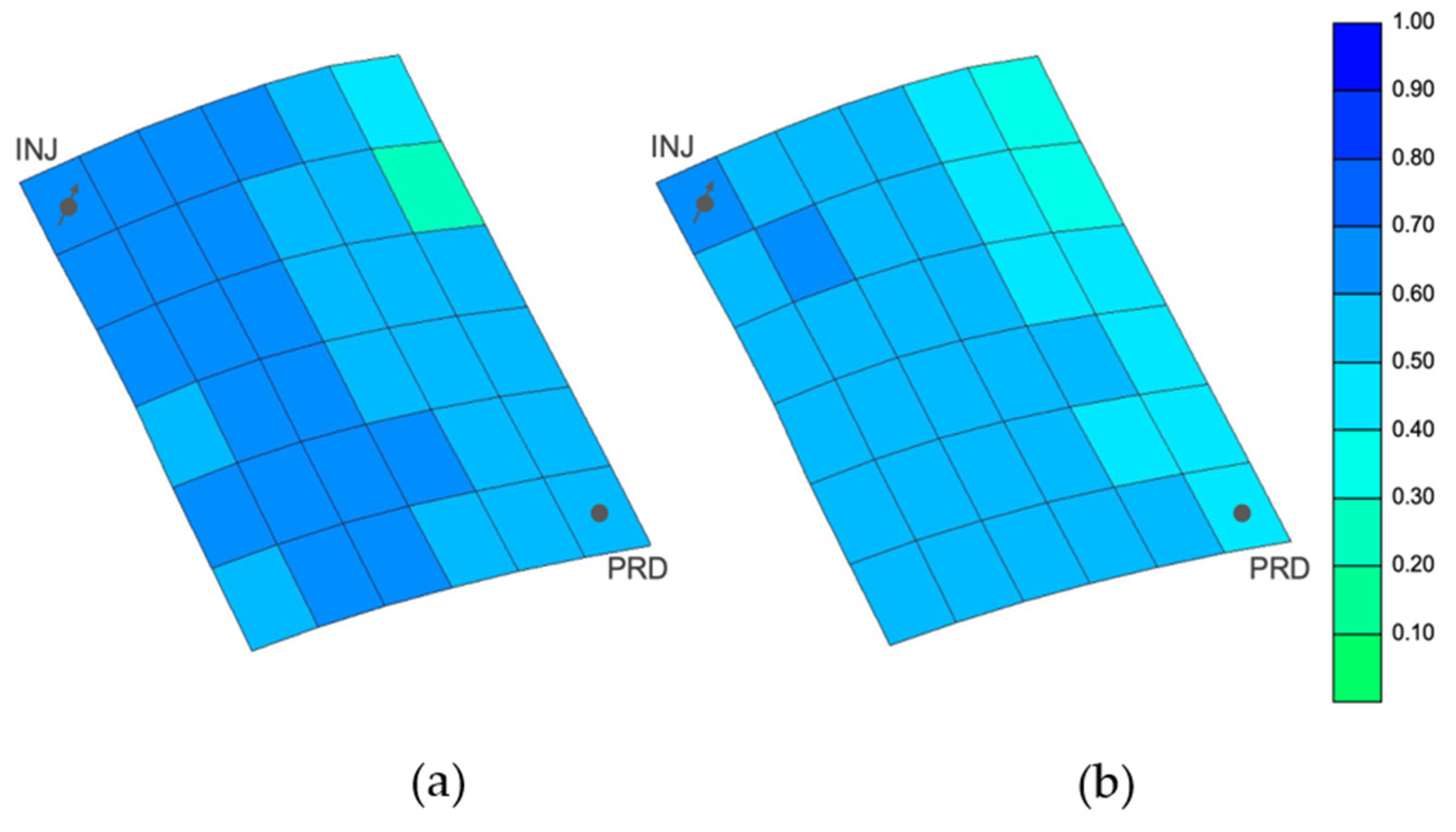
The effects on production with the advanced method were also compared through the average water saturation per year of production (Figure 15). In this plot, we see an improvement of the EWI that reached higher percentages of water saturation. Therefore, we can conclude that by using the EWI method the water ended up covering a larger area of the reservoir, avoiding fingering effects. This can also be observed in the plane 17 of the simulation model at the end of production (Figure 16). More specifically, through the final water saturation in each cell, we can observe that EWI had a better performance.
The integration of Hybrid Machine Learning technology into the pipeline of reservoir simulation with Engineered Water Injection (EWI) using commercial software such as that provided by CMG has been shown to simplify the process and require fewer specific data for predicting petrophysical behavior changes in the tested system. Nowadays, the geochemical background, ionic reactions, and the specific effects to be modeled are obtained by thoroughly testing prior to the simulation. This detailed process represents the current state-of-the-art for Low Salinity/Engineered Water Injection (LSWI/EWI) [7,8]. Incorporating HML into the simulation pipeline allows for the development of accurate models, predicting complex system behavior. This is especially important for EWI cases, where the fluid and rock interactions are highly complex.
Overall, the HML approach simplifies the representation of geochemical effects during the injection of engineered water. This supports the idea of utilizing new technologies to improve the simulation of the behavior of real systems. Machine Learning technologies play an important role in this process, but laboratory analysis remains necessary to obtain precise data. Nevertheless, the HML approach provides the advantage of easy modeling with fewer data, simple implementation, and rapid deliverability of information, thereby allowing for a more informed understanding of petrophysical behavior. Consequently, technology can facilitate better decision making by testing multiple scenarios and ultimately lead to improved recovery of hydrocarbons from reservoirs.
4. Conclusions
In the initial step, the K-Means results allowed the exploration of Kr profiles and led to the conclusion that clustering processes preserve the main three wettability conditions (based on Craig’s [17] qualitative analysis). Subsequently, the trained neural network using data from each cluster was more accurate in predictions. Thus, the Hybrid Machine Learning approach proved to be a better combination for improving the precision of the forecast while retaining the generalization capability (K-Means classification). Furthermore, the application of Grid Search in the ANNs contributed to a significant increase in prediction performance. However, its computation effort needs to be considered in the project schedule.
In the optimization stage, the EOR method resulted in a 45.3% increase in NPV compared to seawater injection. These results indicate an increase in oil recovery and a significant reduction in water production and injection. Despite the higher injection cost of EWI (25% increase), the NPV comparison confirms the method’s efficiency due to the decrease in water expenses. This is supported by the reservoir water saturation history (Figure 14), in which the EWI water saturation is higher than that of waterflooding. The optimal salinity converged to a final concentration of sulfate, calcium, and sodium above the lower standards. Therefore, these results strongly suggest that the use of higher salinity boundaries in the optimization process is crucial for achieving an ideal composition, rather than focusing exclusively on low salinity.
Author Contributions
Conceptualization, L.F.R.; Methodology, L.F.R., R.d.S.G. and M.A.S.; Software, M.A.S.; Validation, M.A.S.; Formal analysis, R.d.S.G.; Data curation, L.F.R. and R.d.S.G.; Writing—original draft, L.F.R.; Writing—review & editing, M.A.S.; Visualization, L.F.R.; Project administration, M.A.S. All authors have read and agreed to the published version of the manuscript.
Funding
This research was funded by Petrobras, under the ANP R&D levy as “Compromisso de Investimentos com Pesquisa e Desenvolvimento” grant number 3105, project title: “Projeto de Molhabilidade e Propriedades Petrofísicas de Rochas Carbonáticas e sua Relação com a Recuperação de Hidrocarbonetos”.
Data Availability Statement
The data associated with this research article is unavailable for public sharing due to privacy considerations and restrictions. For any inquiries or further information regarding the research, please contact the corresponding author.
Acknowledgments
The authors would like to thank LASG (Laboratory of Petroleum Reservoir Simulation and Management), InTRA (Integrated Technology for Rock and Fluid Analysis), and Escola Politécnica of the Universidade de Sao Paulo. This work was conducted with the ongoing Project registered as “Projeto de Molhabilidade e Propriedades Petrofísicas de Rochas Carbonáticas e sua Relação com a Recuperação de Hidrocarbonetos” (USP/Petrobras/ANP) funded by Petrobras, under the ANP R&D levy as “Compromisso de Investimentos com Pesquisa e Desenvolvimento”. The authors would also like to thank FAPESP (the State of São Paulo Research Foundation) and CMG® and MATLAB® for software licenses.
Conflicts of Interest
The authors declare no conflict of interest. The funders had no role in the design of the study; in the collection, analyses, or interpretation of data; in the writing of the manuscript; or in the decision to publish the results.
References
- Bangert, P. Introduction to Machine Learning in the Oil and Gas Industry. In Machine Learning and Data Science in the Oil and Gas Industry; Elsevier: Amsterdam, The Netherlands, 2021; pp. 69–81. ISBN 978-0-12-820714-7. [Google Scholar]
- Hajizadeh, Y. Machine Learning in Oil and Gas; a SWOT Analysis Approach. J. Pet. Sci. Eng. 2019, 176, 661–663. [Google Scholar] [CrossRef]
- Evans, S.J. How Digital Engineering and Cross-Industry Knowledge Transfer Is Reducing Project Execution Risks in Oil and Gas. In Proceedings of the Offshore Technology Conference, Houston, TX, USA, 7–9 May 2019; p. D022S057R014. [Google Scholar]
- Liu, S.; Zolfaghari, A.; Sattarin, S.; Dahaghi, A.K.; Negahban, S. Application of Neural Networks in Multiphase Flow through Porous Media: Predicting Capillary Pressure and Relative Permeability Curves. J. Pet. Sci. Eng. 2019, 180, 445–455. [Google Scholar] [CrossRef]
- Masoudi, R.; Mohaghegh, S.D.; Yingling, D.; Ansari, A.; Amat, H.; Mohamad, N.; Sabzabadi, A.; Mandel, D. Subsurface Analytics Case Study; Reservoir Simulation and Modeling of Highly Complex Offshore Field in Malaysia, Using Artificial Intelligent and Machine Learning. In Proceedings of the SPE Annual Technical Conference and Exhibition, Virtual, 29 October 2020; p. D041S046R008. [Google Scholar]
- Mohaghegh, S.; Ameri, S. Artificial Neural Network as a Valuable Tool for Petroleum Engineers. Paper SPE 1995, 29220, 1–6. [Google Scholar]
- Mosallanezhad, A.; Kalantariasl, A. Geochemical Simulation of Single-Phase Ion-Engineered Water Interactions with Carbonate Rocks: Implications for Enhanced Oil Recovery. J. Mol. Liq. 2021, 341, 117395. [Google Scholar] [CrossRef]
- Nia Korrani, A.K.; Jerauld, G.R.; Sepehrnoori, K. Coupled Geochemical-Based Modeling of Low Salinity Waterflooding. In Proceedings of the SPE Improved Oil Recovery Symposium, Tulsa, OK, USA, 12 April 2014; p. SPE-169115-MS. [Google Scholar]
- Austad, T.; Shariatpanahi, S.F.; Strand, S.; Aksulu, H.; Puntervold, T. Low Salinity EOR Effects in Limestone Reservoir Cores Containing Anhydrite: A Discussion of the Chemical Mechanism. Energy Fuels 2015, 29, 6903–6911. [Google Scholar] [CrossRef]
- Rostami, P.; Mehraban, M.F.; Sharifi, M.; Dejam, M.; Ayatollahi, S. Effect of Water Salinity on Oil/Brine Interfacial Behaviour during Low Salinity Waterflooding: A Mechanistic Study. Petroleum 2019, 5, 367–374. [Google Scholar] [CrossRef]
- Suleimanov, B.A.; Latifov, Y.A.; Veliyev, E.F.; Frampton, H. Comparative Analysis of the EOR Mechanisms by Using Low Salinity and Low Hardness Alkaline Water. J. Pet. Sci. Eng. 2018, 162, 35–43. [Google Scholar] [CrossRef]
- Reginato, L.F.; Pedroni, L.G.; Martins Compan, A.L.; Skinner, R.; Sampaio, M.A. Optimization of Ionic Concentrations in Engineered Water Injection in Carbonate Reservoir through ANN and FGA. Oil Gas Sci. Technol. 2021, 76, 13. [Google Scholar] [CrossRef]
- Brooks, R.H.; Corey, A.T. Hydraulic Properties of Porous Media; Colorado State University: Fort Collins, CO, USA, 1965. [Google Scholar]
- Malekian, A.; Chitsaz, N. Concepts, Procedures, and Applications of Artificial Neural Network Models in Streamflow Forecasting. In Advances in Streamflow Forecasting; Elsevier: Amsterdam, The Netherlands, 2021; pp. 115–147. ISBN 978-0-12-820673-7. [Google Scholar]
- Benchmark Case Proposal Based on a Carbonate Reservoir. Available online: https://www.unisim.cepetro.unicamp.br/benchmarks/br/unisim-ii/overview (accessed on 15 June 2023).
- Correia, M.; Hohendorff, J.; Gaspar, A.T.; Schiozer, D. UNISIM-II-D: Benchmark Case Proposal Based on a Carbonate Reservoir. In Proceedings of the SPE Latin American and Caribbean Petroleum Engineering Conference, Quito, Ecuador, 20 November 2015; p. D031S020R004. [Google Scholar]
- Craig, F.F., Jr. The Reservoir Engineering Aspects of Waterflooding. N. Y. AIME 1971, 3, 562. [Google Scholar]
- Mirzaei-Paiaman, A. New Methods for Qualitative and Quantitative Determination of Wettability from Relative Permeability Curves: Revisiting Craig’s Rules of Thumb and Introducing Lak Wettability Index. Fuel 2021, 288, 119623. [Google Scholar] [CrossRef]
Figure 1.
KrModule schema.

Figure 2.
Hybrid Machine Learning pipeline overview.

Figure 3.
PSO with HML coupling workflow.

Figure 4.
Reduced Unisim-II model.

Figure 5.
PCA plot segmented by clusters.

Figure 6.
Elbow analysis in K-Means.

Figure 7.
Silhouette analysis plot.

Figure 8.
Centroids’ clusters as relative permeability curves.

Figure 9.
Net 00 R2 score vs. hidden layers number using Grid Search CV. Highlighted in red is the neural network configuration, with the highest performance score.
Figure 9.
Net 00 R2 score vs. hidden layers number using Grid Search CV. Highlighted in red is the neural network configuration, with the highest performance score.

Figure 10.
Net 00 R2 score vs. hidden layers number using Grid Search CV.

Figure 11.
Comparison of Kr curve predicted by each network (in green) and actual curves (in black): (a) comparison plot curve from 00 cluster; (b) comparison plot curve from 01 cluster; (c) comparison plot curve from 02 cluster.
Figure 11.
Comparison of Kr curve predicted by each network (in green) and actual curves (in black): (a) comparison plot curve from 00 cluster; (b) comparison plot curve from 01 cluster; (c) comparison plot curve from 02 cluster.

Figure 12.
Percent volume of fluids.

Figure 13.
Optimized injection salinity.

Figure 14.
Relative permeability after optimization vs. original.

Figure 15.
Average reservoir water saturation with EWI vs. waterflooding.

Figure 16.
Comparison of water saturation in the 17th reservoir horizontal plane after 30 years of production as of 23/09/2046. (a) Engineered Water Injection and (b) waterflooding.
Figure 16.
Comparison of water saturation in the 17th reservoir horizontal plane after 30 years of production as of 23/09/2046. (a) Engineered Water Injection and (b) waterflooding.


Table 1.
Wells’ operational conditions, adapted from [16].
Table 1.
Wells’ operational conditions, adapted from [16].
| Type | Vertical Producer | Vertical Injection |
|---|---|---|
| Max. water rate (m3/day) | - | 5000 |
| Max. oil rate (m3/day) | 20 | - |
| Max. liquid rate (m3/day) | 2000 | - |
| BHP (kgf/cm2) | Min 190 | Max 350 |
Table 2.
Economic scenario for reduced model [12].
Table 2.
Economic scenario for reduced model [12].
| Type | Variables | Value |
|---|---|---|
| Price (USD/STB) | Oil | 54.76 |
| Gas | 0.70 | |
| Cost (USD/STB) | Oil production | 10.952 |
| Gas production | 0.4675 | |
| Water production | 1.1 | |
| Engineered water injection | 1.98 | |
| Water injection | 1.1 | |
| Investment (USD millions) | Drilling and completion vert. well | 22.8/m |
| Connection vertical well platform | Data | |
| Platform | Equation |
Table 3.
PSO in KrModule configuration.
| PSO Features | Values |
|---|---|
| Particle number | 10 |
| Interaction number | 12 |
| Exploration factor (K) | 1 |
| Cognitive component (φ1) | 2.05 |
| Social component (φ2) | 2.05 |
| Damping factor (Wdamp) | 1 |
| Constriction coefficient (chi) | Equation (4) |
Table 4.
Grid Search CV with final optimization in each case.
| Hyperparameters | Net 00 | Net 01 | Net 02 |
|---|---|---|---|
| Hidden layer size | 12 | 10 | 11 |
| Activation | logistic | logistic | logistic |
| Solver | lbfgs | lbfgs | lbfgs |
| Learning rate | adaptative | adaptative | adaptative |
Table 5.
Fluid production, recovery factor, and final NPV from optimum cases.
| Oil Produced (105m3) | Water Produced (105m3) | Water Injected (105m3) | Oil Recovery Factor (%) | Final NPV (MMUS) | |
|---|---|---|---|---|---|
| Water | 15.72 | 15.35 | 40.03 | 38.01 | USD 18.21 |
| EWI | 16.88 | 9.13 | 28.60 | 41.4 | USD 26.45 |
Table 6.
Optimized variable results.
| Inj. Rate (m3/Day) | Inj. Pres. (m3/Day) | Prd. Rate (m3/Day) | Prd. Pres. (m3/Day) | SO42− (ppm) | Ca2+ (ppm) | Cl− (ppm) | Mg2+ (ppm) | Na+ (ppm) |
|---|---|---|---|---|---|---|---|---|
| 2091.66 | 33,256.36 | 1994.73 | 996.73 | |||||
| 2878.92 | 33,565.98 | 1995.80 | 989.79 | 1493.01 | 4933.7 | 198.64 | 800.63 | 14,951.14 |
Disclaimer/Publisher’s Note: The statements, opinions and data contained in all publications are solely those of the individual author(s) and contributor(s) and not of MDPI and/or the editor(s). MDPI and/or the editor(s) disclaim responsibility for any injury to people or property resulting from any ideas, methods, instructions or products referred to in the content. |
© 2023 by the authors. Licensee MDPI, Basel, Switzerland. This article is an open access article distributed under the terms and conditions of the Creative Commons Attribution (CC BY) license (https://creativecommons.org/licenses/by/4.0/).
Share and Cite
MDPI and ACS Style
Reginato, L.F.; Gioria, R.d.S.; Sampaio, M.A. Hybrid Machine Learning for Modeling the Relative Permeability Changes in Carbonate Reservoirs under Engineered Water Injection. Energies 2023, 16, 4849. https://doi.org/10.3390/en16134849
AMA Style
Reginato LF, Gioria RdS, Sampaio MA. Hybrid Machine Learning for Modeling the Relative Permeability Changes in Carbonate Reservoirs under Engineered Water Injection. Energies. 2023; 16(13):4849. https://doi.org/10.3390/en16134849
Chicago/Turabian StyleReginato, Leonardo Fonseca, Rafael dos Santos Gioria, and Marcio Augusto Sampaio. 2023. "Hybrid Machine Learning for Modeling the Relative Permeability Changes in Carbonate Reservoirs under Engineered Water Injection" Energies 16, no. 13: 4849. https://doi.org/10.3390/en16134849
Note that from the first issue of 2016, this journal uses article numbers instead of page numbers. See further details here.