


Kriging-Assisted Multi-Objective Optimization Framework for Electric Motors Using Predetermined Driving Strategy


1
Vehicle Industry Research Center, Széchenyi István University, Egyetem Tér 1, 9026 Győr, Hungary
2
Department of Mathematics and Computational Sciences, Széchenyi István University, Egyetem Tér 1, 9026 Győr, Hungary
*
Author to whom correspondence should be addressed.
Energies 2023, 16(12), 4713; https://doi.org/10.3390/en16124713
Submission received: 16 May 2023
/
Revised: 9 June 2023
/
Accepted: 12 June 2023
/
Published: 14 June 2023
(This article belongs to the Special Issue New Solutions in Electric Machines and Motor Drives)
Abstract
:In this paper, a multi-objective optimization framework for electric motors and its validation is presented. This framework is suitable for the optimization of design variables of electric motors based on a predetermined driving strategy using MATLAB R2019b and Ansys Maxwell 2019 R3 software. The framework is capable of managing a wide range of objective functions due to its modular structure. The optimization can also be easily parallelized and enhanced with surrogate models to reduce the runtime. The framework is validated by manufacturing and measuring the optimized electric motor. The method’s applicability for solving electric motor design problems is demonstrated via the validation process. A test application is also presented, in which the operating points of a predetermined driving strategy provide the input for the optimization. The kriging surrogate model is used in the framework to reduce the runtime. The results of the optimization and the framework’s benefits and drawbacks are discussed through the provided examples, in addition to displaying the properly applicable design processes. The optimization framework provides a ready-to-use tool for optimizing electric motors based on the driving strategy for single- or multi-objective purposes. The applicability of the framework is demonstrated by optimizing the electric motor of a world recorder energy-efficient race vehicle. In this application, the optimization framework achieved a 2% improvement in energy consumption and a 9% increase in speed at a rated DC voltage, allowing the motor to operate at desired working points even with low battery voltage.
1. Introduction
High power density and high efficiency are important for electric motors applied in electric and hybrid vehicles, while available space and energy consumption are limited in these applications. These requirements are best obtained using permanent magnet synchronous machines (PMSMs) in low-power applications. The structure of PMSMs was analyzed for low-power applications in Ref. [1], where the effects of surface-mounted and interior-mounted PMSMs were studied. This paper presents a kriging-assisted multi-objective optimization framework for electric motors and its validation, as well as a test application. The details of the framework have been presented in Ref. [2], describing various example applications, but its comparison and validation with measurement results are presented here for the first time. Furthermore, this is the first application of the framework where optimization is performed for a predetermined driving strategy.
In addition to the basic PMSM structure, many other design variables can impact motor performance. Numerous papers on electric motor optimization can be found in the literature. The energy optimization of a brush-phase asynchronous motor at different load levels is presented in Ref. [3]. To minimize the energy loss at start-up, it is necessary to control the start voltage and frequency as a function of the load torque within a given start time interval. The optimal voltages and frequencies at different load torque levels are determined using the particle swarm optimization (PSO) algorithm. Based on the outputs of PSO, a neuro-fuzzy system design is proposed for proper control of the inverter during motor start-up.
In Ref. [4], an efficient multi-objective optimization algorithm is presented through the optimization of an asynchronous motor. A gravitational search algorithm (GSA) is used in that work. The objective functions aim to minimize losses and maximize torque, using an existing motor as a starting point.
The multi-objective optimization of PMSMs and the application of the PSO algorithm with a kriging surrogate model is presented in Ref. [5]. The kriging surrogate model can provide estimations, reducing the need for expensive evaluations of the objective function. Simulation is only necessary for motor models that perform well during preliminary evaluations.
Based on these results, the MATLAB built-in classical genetic algorithm (GA) is chosen with a kriging surrogate model for the optimization algorithm of the framework. However, due to the modular design of the framework, it can be easily replaced by any other heuristic model.
A multi-objective optimization design, duty-cycle model predicates the current control and performance verification of an outer-rotor PMSHM for a low-speed direct drive EV, which is shown in Ref. [6]. This also concerns workpoint-based electric motor optimization for vehicle drives, validated by measurement results. Ref. [7] presents a similar system, but here, a more efficient multi-objective optimization algorithm is used. In Ref. [8], a single-objective optimization algorithm is improved to handle multiple objective functions.
The framework presented in our paper is a general design tool suitable for various applications. The applications shown in this paper involve a variety of objective functions, design variables, and constraints. Therefore, our goal is to create a tool suitable for as general a set of tasks as possible.
2. Methodology
In multi-objective optimization, the goal is to minimize or maximize several variables (e.g., mass and losses) simultaneously. Analytical methods are often unable to handle the problems presented while evaluating electric motors for vehicles, or they are only capable with a relatively high error rate. Maxwell’s equations describing the electrodynamic processes need to be solved using numerical methods to determine some objective functions (such as loss calculation). For these calculations, the optimization framework uses the Ansys Maxwell 2019 R3 software.
2.1. The Calculation of the Mass
The mass of the motor is given by the cross-section of the components in its two-dimensional FEM model, the length of the motor and the density of the components, meaning the mass of the winding head is neglected.
2.2. The Calculation of the Losses
The motor losses are calculated using a combination of analytical methods within the MATLAB optimization framework and electrodynamic simulations performed using ANSYS Maxwell 2019 R3 finite element simulation software. The total losses calculated for a motor are the combined sum of the iron and winding losses calculated at the various operating points.
Iron loss refers to both the power dissipation resulting from hysteresis caused by rapid changes in the current direction within the coil, as well as the power dissipation from eddy currents induced by permanent magnets in a changing magnetic field. Winding loss represents the ohmic loss resulting from the current flowing through the motor winding.
2.3. The Optimization
Mathematical optimization is used to solve problems that cannot usually be solved using analytical methods, such as when the optimal parameter combination in a single or multi-variate space needs to be found, given predefined constraints, where the value of the objective function is extremal. This extremization is usually a minimization or maximization of the value of the objective function [9].
2.4. The Multi-Objective Optimization
In situations when more than one objective function needs to be optimized, it is not always possible to conclude that one individual is unquestionably superior compared to another. Reducing the problem to single-objective optimization using a winding loss weighted average of the objective values is the simplest technique to handle this issue.
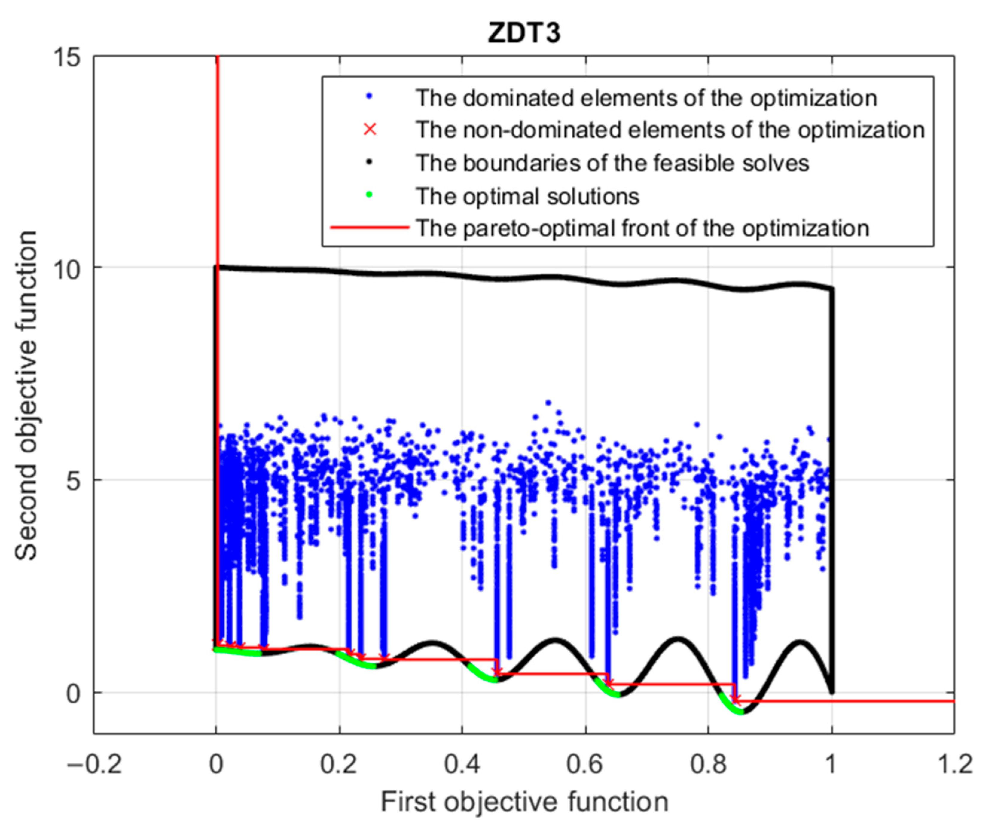
In other approaches, the evaluated individuals can be divided into two parts, dominated and non-dominated. For a problem with several objective functions, an individual can only be clearly superior to another individual if the other individual dominates it, for example, when the total objective function value is closer to the optimum. Individuals that have a clearly superior individual are called dominated individuals, while others without it are called non-dominated. The non-dominated individuals form a front in each generation; these are the best individuals of that generation. The front created by the non-dominated individuals of the last generation is the Pareto front in the space of the multi-dimensional objective function, as shown in Figure 1.
The test function’s specifics are provided in Ref. [10] as ZDT3. The space bounded by the design variables and constraints is shown in the picture with a black line. The green portion of the envelope curve for this field represents the ideal pareto front. The minimization of both objective functions is the optimization’s goal; this region is situated to the left of the field’s edge. As seen in the illustration above, a concave field could include several portions. An approximation of this optimal pareto front is obtained by performing a multi-objective optimization. The beginning of the pareto front approximation created as an outcome of the optimization procedure is shown by the red × sign. Since there is no better individual according to objective functions, they are referred to as non-dominated individuals. The blue dots represent the dominated individuals, since they are dominated by better individuals according to all objective functions.
2.5. The Genetic Algorithm
The genetic algorithm is included in the evolutionary mathematical optimization. Its name comes from the similarity of its operation to that of genetics, the science of heredity. Genes in the human body contain all the structural and functional information of the body’s proteins. These genes are hereditary, meaning that descendents inherit the genes they receive from their parents. These genes can be inherited one-to-one, crossed with each other or through mutation. This gives the descendant the unique traits in addition to those inherited from the parents. Genetic algorithms operate based on this logic [9].
Genetic algorithms always start the optimization from an initial population. The individuals in the initial population can be predetermined or randomized. However, for the algorithm to work properly, the initial population must be sufficiently large and sufficiently diverse. This is the so-called generation zero, the top parental level of the optimization, from which further generations can be constructed. The algorithm runs its objective function evaluation code over the individuals and ranks them on this basis. The problem is no longer trivial if there are multiple objective functions to rank. The best individuals are then passed on one by one to the next generation of individuals. The combination of the parameters of the other individuals is used to produce new individuals for the next generation by a crossing algorithm or by changing each individual, for example, via a mutation algorithm. It is important to ensure that the new individuals satisfy the limitations given by the optimization, i.e., that the parameter combinations lie inside the n-dimensional space (where n is the number of parameters in the parameter combinations) during mutation and crossover. Once the new generation is prepared, the evaluation of objective functions needs to be performed on it as well. Then, the new generation can be started from these. This process will continue for the number of generations we define, but after a while, the new generation will not be diverse enough, from which point, the optimization can no longer work efficiently. This state will certainly occur, but it can be delayed, ending up closer to the global optimum by choosing the right size and individuals of the initial population. The parameters of the optimization are the size of the initial population (and indirectly its individuals), the number of generations to be produced and the choice of mutation and crossing algorithms.
In multi-objective optimization, the results are ranked. Feasible individuals are assigned ranks iteratively. Rank 1 individuals are not dominated by any other individuals. Rank 2 individuals are only dominated by rank 1 individuals. In general, rank k individuals are only dominated by individuals in rank k − 1 or lower. This implies that individuals are ranked based on their distance from the current pareto front.
2.6. The Kriging Surrogate Model
The assistant algorithm replaces the internal computational models of the multi-objective optimization environment. The optimization algorithm first passes the parameters to the assistant algorithm, which provides an expected value, a lower bound and an upper bound in response to each objective function value using an analytically solvable method. When minimizing the objective function values, it is necessary to check whether this lower bound is below any objective function value calculated so far (using FEM). The actual evaluation of the objective function is initiated if this condition is true for either of the objective function values. Otherwise, the optimization algorithm utilizes the expected value of the objective function values as input for the design parameters of the subsequent motor models [2].
3. The Optimization Framework
The optimization framework is suitable for the operating-based optimization of electric motors. The working points consist of torque demand, speed, and time weighting. These operating points can be acquired from a predefined duty cycle of the investigated vehicle.
3.1. The Workflow of the Optimization Framework
The optimization framework requires an associated optimization algorithm to operate. The inputs to the framework are the parameter vectors provided by the optimization algorithm, a database of previous results and data of the operating points. Transmission and other losses that are considered constant are not considered in the framework. The outputs of the framework are the objective function values.
The optimization framework receives input from the optimization algorithm and the design variables of the new generation of individuals after checking constraints.
These parameters are first obtained via the kriging surrogate model, which gives an estimate of the objective function values based on the results of previous evaluations. If the estimation suggests that the model is likely to be one of the non-dominated individuals, then the actual evaluation is performed; otherwise, the values of the estimation are returned as target function values to the optimization algorithm. Since the optimization carries the best individuals from one generation to the next, the previous evaluation results are checked to see if an actual evaluation has already been performed with the given parameter combination. If such a previous evaluation exists, the results from that evaluation are utilized.
If the actual evaluation is started, the implicit variables are calculated from the parameters. These are variables that are defined by the working and design variables. The operating point parameters are predefined parameters whose values do not change during the optimization.
Once all the necessary inputs are ready to evaluate the motor model, the torque iteration starts. This is necessary because in the Ansys Maxwell 2019 R3 FEM software, the inputs are the speed and excitation current, while the operating points are speed and torque demand, so an iterative sequence of runs is required to determine the current value for a given torque. Since the optimization algorithm already performs one run when checking the constraints, the data obtained from this run can be used to reduce the number of iterations required (in many cases, it is effectively 1). Since the torque has six periods in one electrical turn, it is sufficient to simulate one sixth electrical turn. A more expensive simulation of two electrical turns is required for the loss calculation because of the initial transient stages.
After the determination of the excitation current amplitude, the evaluation of the actual motor model is performed, which consists of the FEM model and the evaluation algorithm attached to it. This model calculates the mass and losses of the motor.
The loss capacities of the motor at different operating points and the product of the time weights give the calculated energy loss per operating point, and the sum of these gives the calculated energy loss for the motor.
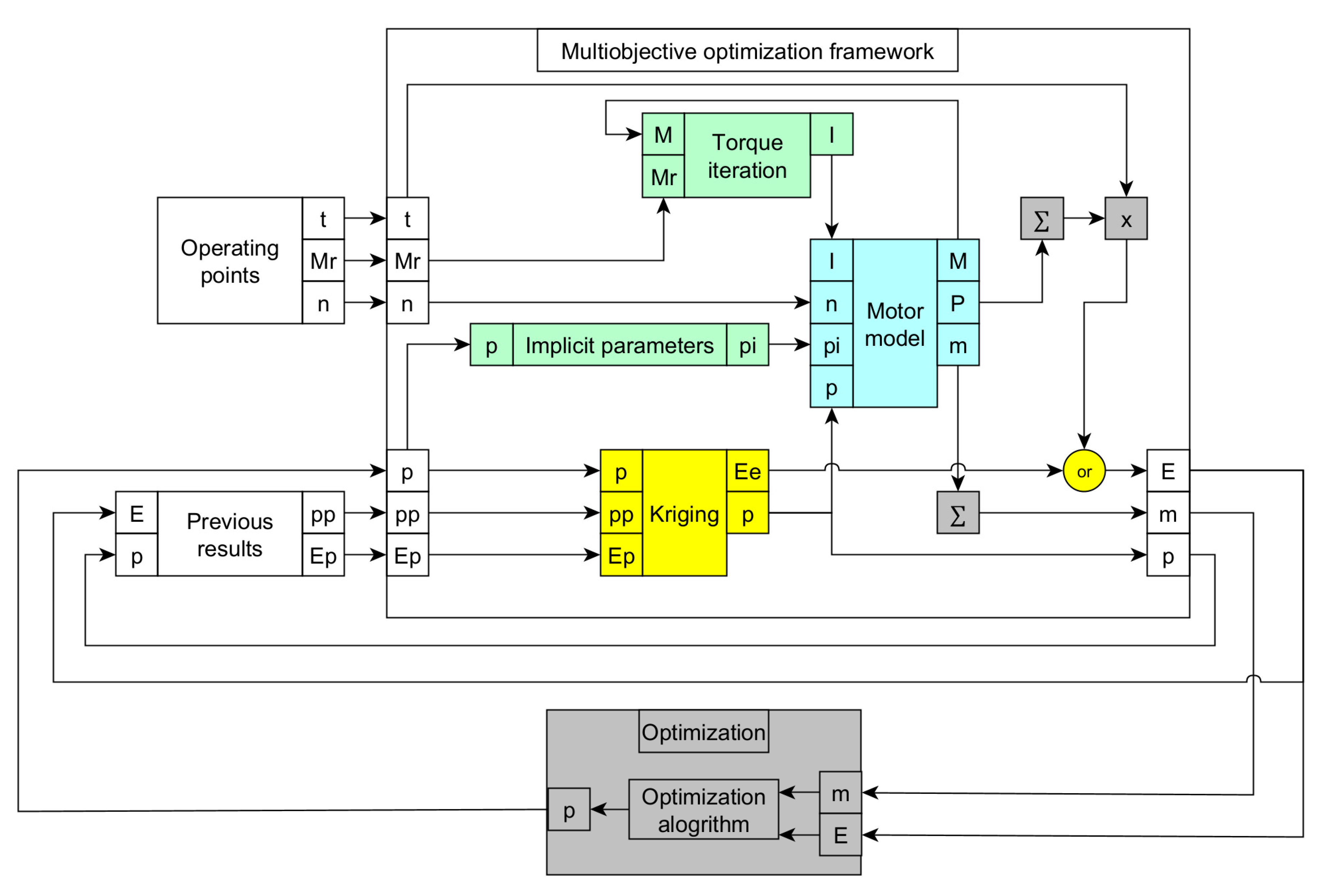
The structure of the optimization framework is shown in Figure 2. As an example, the two objective functions are energy loss and mass. In this example, only the loss calculation is accelerated by the assistant algorithm since no time-consuming calculations are needed for the mass calculation. The legend of Figure 2 is summarized in Table 1.
The operational loop of the optimization framework is illustrated in this block diagram. Initially, in the first step, the framework only receives the parameter vectors of the initial population and does not have any previous results. The optimization process continues until one of the predefined criteria is met. This criterion can be the maximum number of generations, the maximum time, the rate of improvement compared to previous generations and so on. When this criterion is met, the optimization box ceases to send new parameter vectors to the framework and the process terminates.
3.2. The Motor Model
The motor model consists of an FEM model built in ANSYS Maxwell and the dedicated MATLAB code structured into it. The FEM simulation is a fixed-speed transient analysis with excitation current input.
A motor model is already required for the verification of constraints. Since we are talking about motors for vehicle propulsion, there is always a voltage and a current limit and an expected peak power. In practice, this means that a motor design will only pass the constraint inspection if it can deliver the torque corresponding to the intended corner point at the corresponding speed for a given battery voltage and current limit. In addition to torque and losses, the FEM model can also calculate induced voltages, thus allowing the minimum DC voltage associated with the excitation current to be calculated. The calculation of this process and the winding loss is carried out in the dedicated MATLAB code.
Validation of Motor Model
The validation of the FEM model was necessary to perform to check the proper function of the model. The validation needed to be completed before application of the model in the optimization framework. The model was validated using the state-of-the-art FEM model which analyzed in Ref. [11]. The meshed view of the FEM model is shown in Figure 3.
The torque of the state-of-the-art model and the validation model at the operation point at 3000 rpm and 250A excitation current can be seen in Figure 4.
The two torque functions are almost identical, with only a minimal difference. Based on these results, the accuracy of the ANSYS Maxwell 2019 R3 finite element software was judged to be adequate with appropriate settings.
3.3. The Validation of the Optimization Framework through an Application
In this application, the objective was to create an electric motor for the SZEnergy team at Széchenyi István University. This team has built a race vehicle for Shell Eco-marathon (SEM) energy efficiency competition. This validation was made for the vehicle edition created for SEM 2016. An electric motor was required to drive the vehicle so that it could complete the race by utilizing the least amount of energy possible while maintaining the motor’s mass, based on the identified vehicle, track and driving strategy. As a motor is in constant contact with the wheel, it was also important to ensure that it could run freely with low resistance and that the torque fluctuation was also minimized—the objective functions were therefore the motor’s energy loss, torque fluctuations and mass, which were minimized during the optimization.
As the FEM model employs transient simulations, the calculated results were time-dependent; for this reason, it was feasible to compute quantities such as torque fluctuations during the post-processing step.
3.3.1. Motor Model for Validation
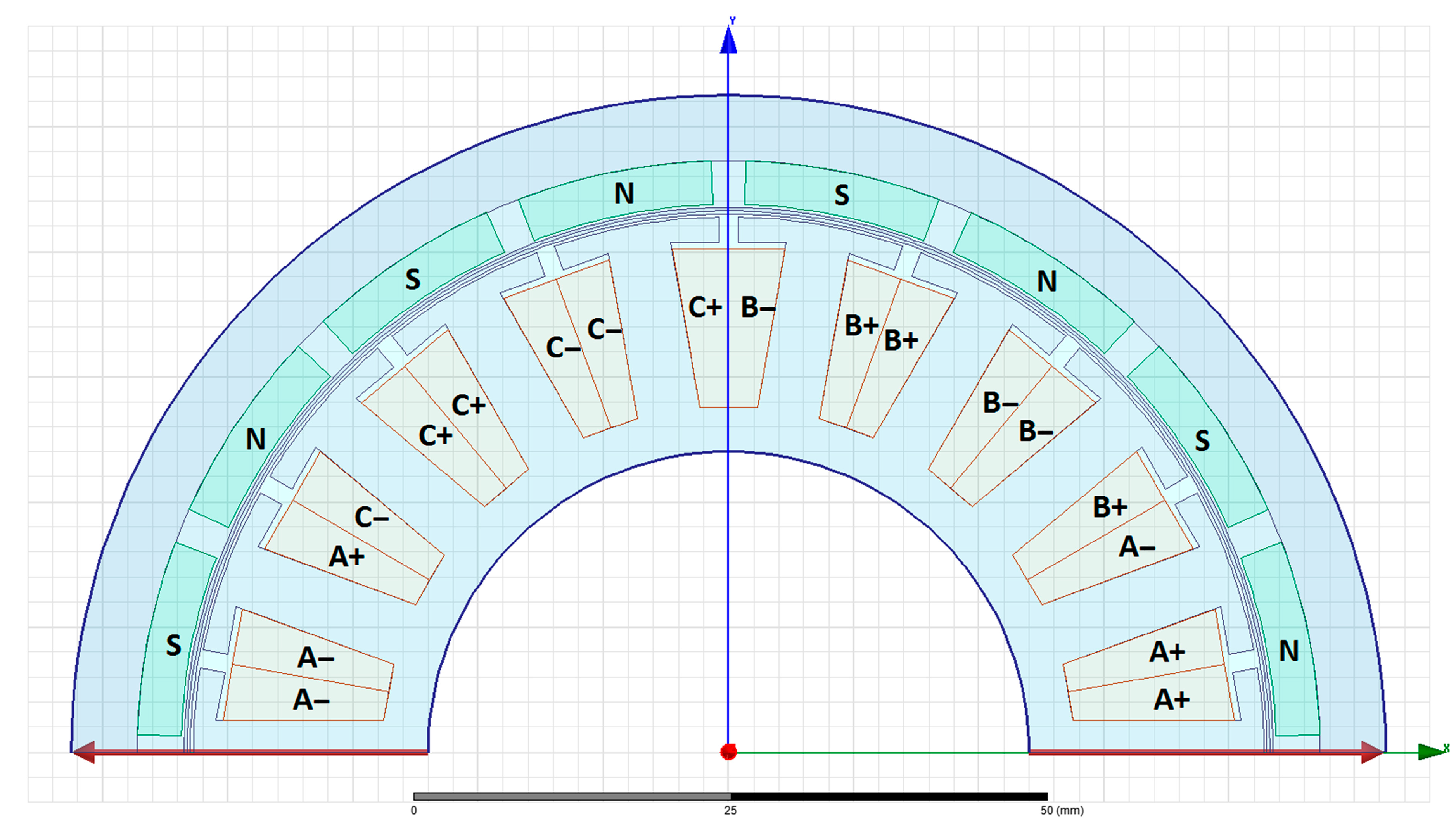
As the motor was directly driving the vehicle, an external rotor PMSM was needed. The motor has a fractional number of slots, 8 pairs of poles and 18 slots to reduce torque losses. These parameters were not part of the optimization. The construction and winding of the motor are shown in Figure 5.
The two lower edges of the 2D model have periodic rotational symmetry, and the outer and inner edges have a zero-vector potential boundary condition. The material of the magnets is neodymium (NdFe35), the winding is copper and the stator and rotor are plated iron (M19_29G).
3.3.2. The Design Variables and the Operating Points
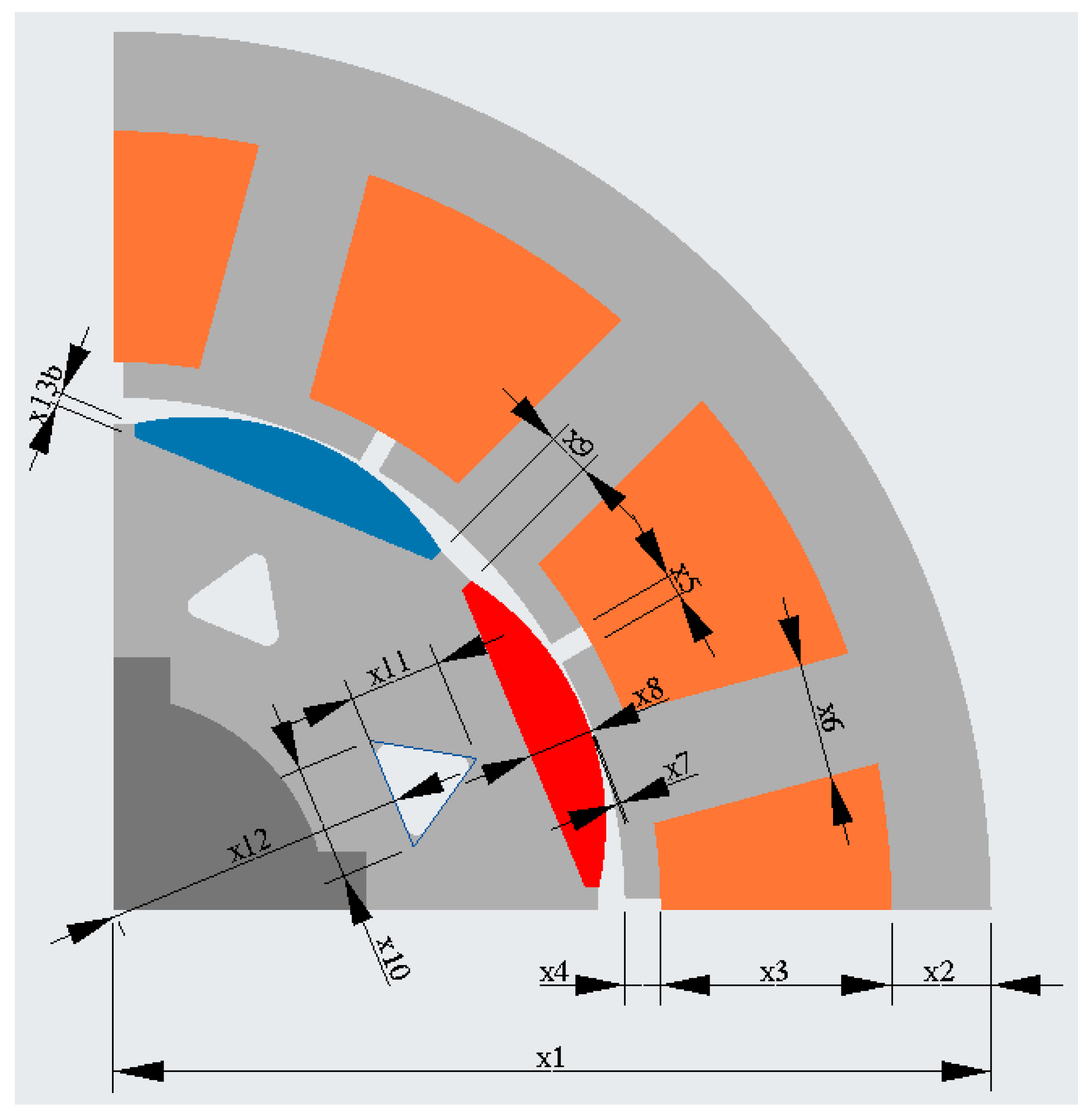
A total of 13 design variables were defined. Of these, 11 were geometric variables (slot dimensions, magnet dimensions, air gap dimensions, motor length and diameters). The remaining two were the number of turns and the wire diameter. Of these, one output quantity was the number of parallel threads. Each design variable also had upper limits. The installation location provided the maximum values for the geometric variables of the enclosure dimensions. To ensure that the geometric constraints only affected a relatively small portion of the feasible parameter space, the upper limits of the other geometric variables were set accordingly. The lower limits of the geometric variables were determined based on considerations of constructability. For the number of turns and wire diameter, wider limits were set. Although this wider range of design variables slowed down the convergence of the optimization algorithm, it allowed the optimization algorithm to search in a larger parameter space. The parameter values for the initial iteration were randomly assigned. The two operating points tested were 270 rpm–8, Nm–800 s and 270 rpm–0 Nm–200 s.
3.3.3. The Constraints
The model had linear and non-linear constraints divided into three levels. If one level failed the verification, the others were not evaluated. The first level included the geometric constraints, where it was checked that the edges of the parts did not interlock and that the minimum material thickness required for mechanical stiffness was presented everywhere.
The second level examined whether the fill factor could be achieved in each slot cross-section and whether the winding could be produced for a given number of threads and wire diameter. If the design passed the inspection by one strand, an iterative process was used to determine how much the number of parallel strands could be increased. The model was given the highest available value as a parameter in each case. Only feasible designs were allowed to reach the third level. Here, it was determined whether the motor could deliver the 20 Nm specified as the corner operating point at 330 rpm with a maximum current limit of 29 A and a battery voltage of 43 V. As with the torque iteration, a shorter simulation was sufficient.
3.3.4. The Parametrization of Optimization Algorithm
Since the simulation of FEM models has a large time demand, it is important to limit the runtime. The best way to maximize the use of this time limit is to identify the best parameter combinations. A case study of an optimization problem that can be solved completely analytically was carried out to establish this.
The model to be optimized consisted of 13 design variables and 3 objective functions. In addition, the design variables were subject to linear and non-linear constraints. The Osyczka and Kundu function consists of six design variables and two objective functions with linear and nonlinear constraints [12].
Preliminary calculations estimate that with the current model, an objective function evaluation takes on average 4 min. The dedicated maximum runtime is 7 days. Including the effect of the kriging surrogate model, about 4–5000 evaluations can be included within this time. The optimization of the test task was carried out with several different sets of parameters. The effective Pareto front was achieved with a population size of 80 and a crossover factor of 0.5 for the given evaluation number. The latter means that new generations are produced with the same proportion of crosses as mutations.
3.3.5. The Results of Optimization
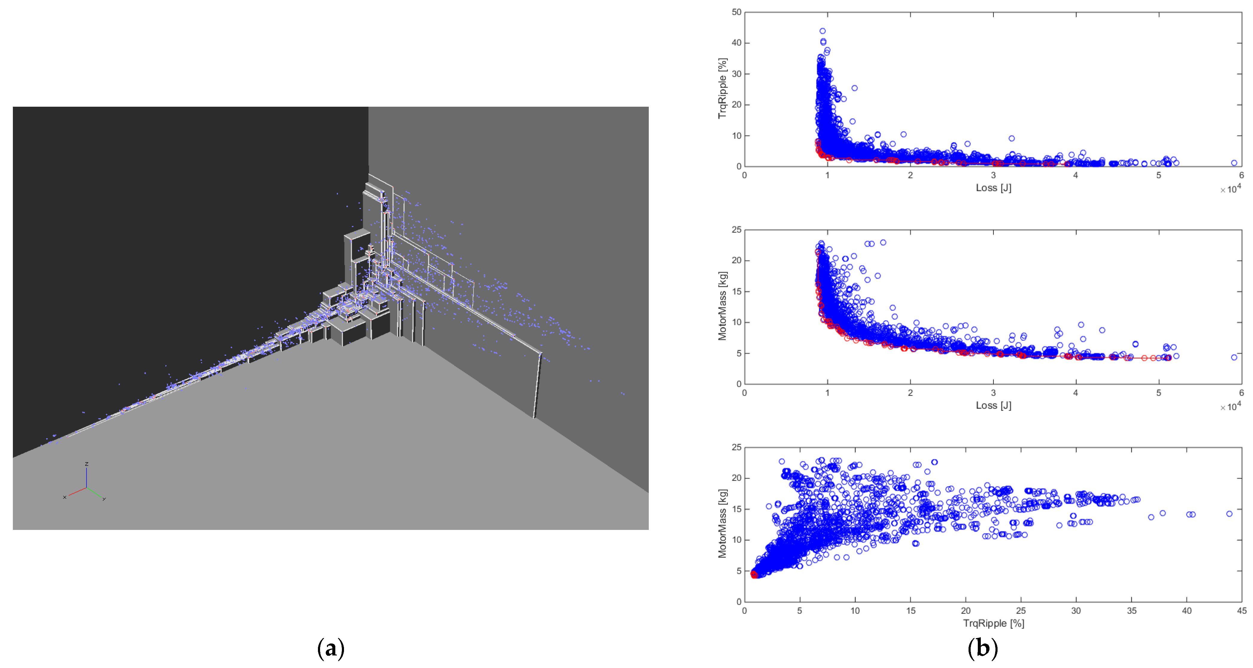
During the optimization, 54 additional generations were run after the initial generation, for a total of 4400 evaluations. The results of the optimization are shown in Figure 6.
In the figure above, blue markers indicate dominated individuals and red markers indicate non-dominated individuals, or in other words, the elements of the pareto front. The 3D result reveals the real pareto front, observed as we look towards the origin from the perspective of the dominated individuals, with the three axes representing the three objective functions. The pareto front of the optimization is depicted by the gray surfaces. In the 2D result, the projection of this structure is presented from three different directions. To ensure clarity, the red markers do not signify the pareto front of the optimization, but they indicate the non-dominated individuals based on either two objective functions. Five of these motor constructions were selected for further analysis. The model selected for production was determined by parameter sensitivity, eccentricity sensitivity and manufacturability tests. The selected motor model is shown in Figure 7 together with the modifications required for fabrication and mounting.
3.3.6. The Validation of the Optimization Framework
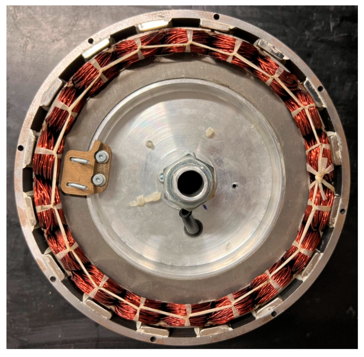
The selected motor was manufactured, making test bench measurements possible. Unfortunately, there were not any suitable instruments available to measure torque fluctuations, but measuring the efficiency map was possible. The manufactured motor is shown in Figure 8.
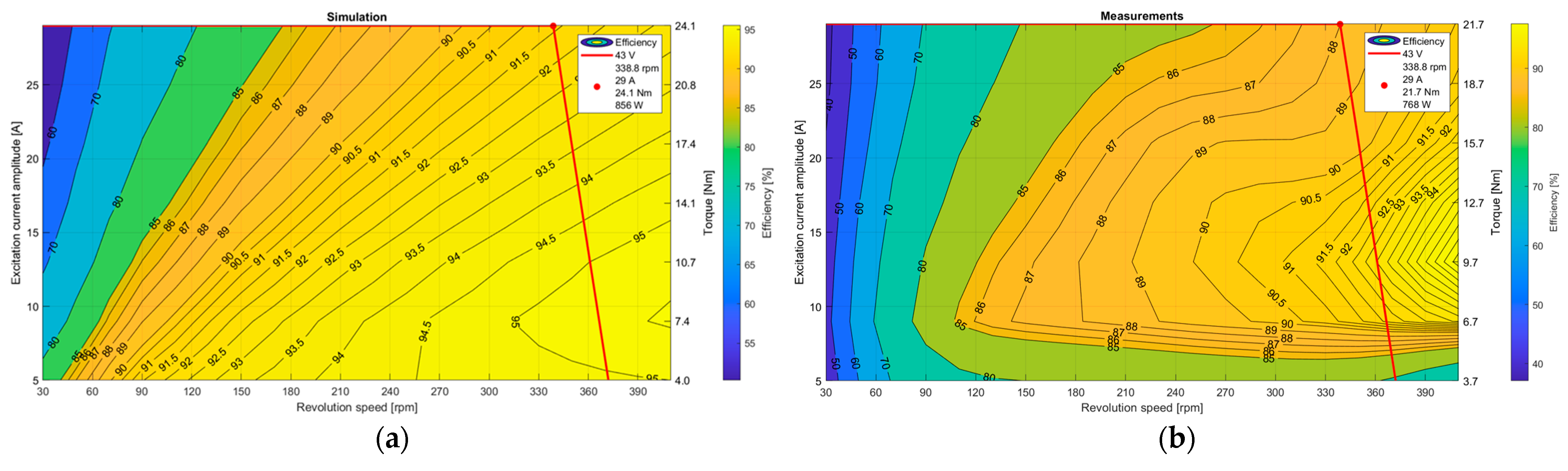
The material properties of the finished motor differ minimally from those in the simulation model, but they do not cause significant differences. The measurements were made in the electric powertrain testbench laboratory of the Széchényi István University. During the test, the input and output power of the motor were measured. The efficiency field calculated from the measurement results was suitable for comparison with simulation results if the motor controller and the mechanical losses were known. These losses were estimated to be between 3% and 5% based on previous measurements. The efficiency map of the simulated motor (a) and measured motor (b) can be seen in Figure 9.
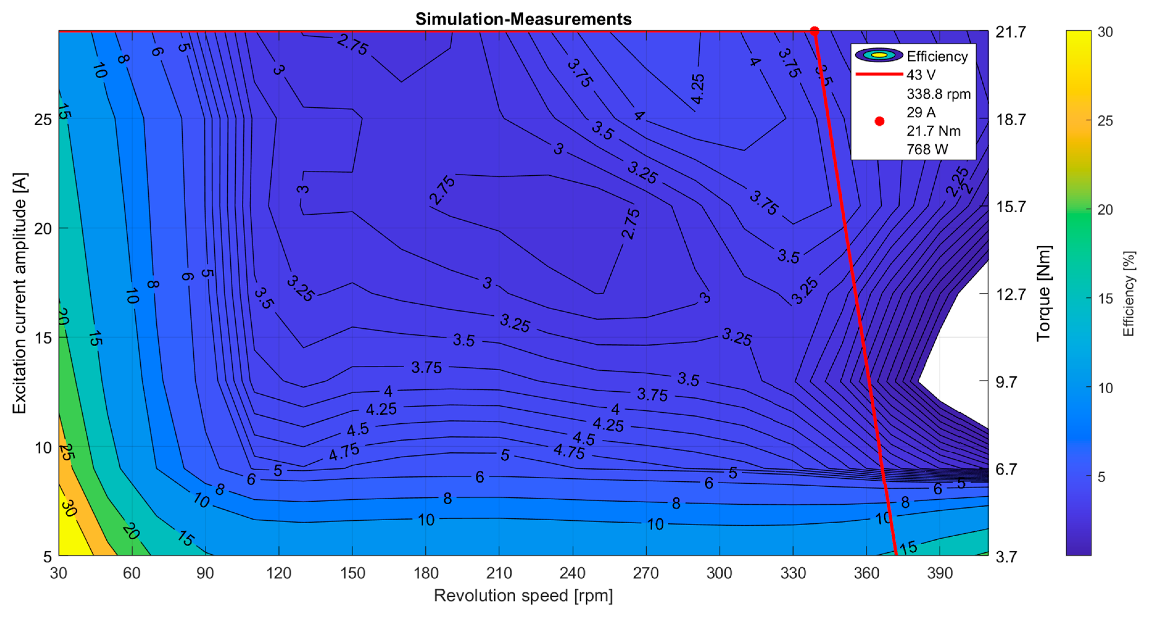
The simulation efficiency field calculation did not consider the losses of the motor controller as well as the mechanical losses, so the measurement results were expected to show lower efficiency. In the higher power ranges, the average deviation of 3–4% is clearly visible, which starts to increase at low loads and low speeds. This is due to the inaccuracy of the measurement, the insensitivity of the braking machine and the higher effect of mechanical losses. The minimum expected corner point is also measured to be achievable, and the most used range (8 Nm—around 270 rpm) is around 90% of efficiency. Figure 10 shows the difference between the simulated and measured efficiency fields.
4. The Application of Optimization Framework
In this application, the electric motor used in the SZEnergy team’s 2022 race vehicle, referred as SZEVOL, was optimized. It is an internal rotor PMSM with 4 pole pairs and 12 slots, rated at 1kW. The rotor and stator are M19_29G marked soft iron laminated, the winding is copper and the magnets are N35 marked neodymium. The material properties were not changed during the optimization. The motor drives the rear left wheels of the vehicle with the ratio of 3.273. This deceleration ratio is achieved by a synchronous belt connection with an average efficiency of 97%. In addition, the motor is driven by a team-built motor controller, with 95% average efficiency in the commonly used operating points. In the evaluation of the optimization results, the efficiency of the belt drive and the motor controller are considered constant.
The optimization aims to increase the efficiency of the motor and reduce the energy demand of the vehicle. The driver of the vehicle is also assisted by a predetermined driving strategy during the race, so the operating points for the motor optimization are given. The driving strategy optimization was performed by using a measurement-based vehicle model, which simulates the behavior of the race vehicle by modeling the resistance losses in straights and in corners as well. The powertrain model in that case was changed from the original test bench measured model to the simulated model of SZEVOL. This change could be made due to the application of a validated FEM model. The track characteristics of TT Circuit Assen were considered in the optimization, which was made according to the problem formulation of the Max TRQ method [13,14].
4.1. The Objective Functions and the Design Variables
It is essential to keep a vehicle’s mass at a constant level to improve its consumption; therefore, the optimization aimed not only to reduce the losses but also to reduce the mass of the motor. Based on that, the optimization had two objective functions and sixteen design variables altogether.
4.2. The Simulation Results of the SZEVOL
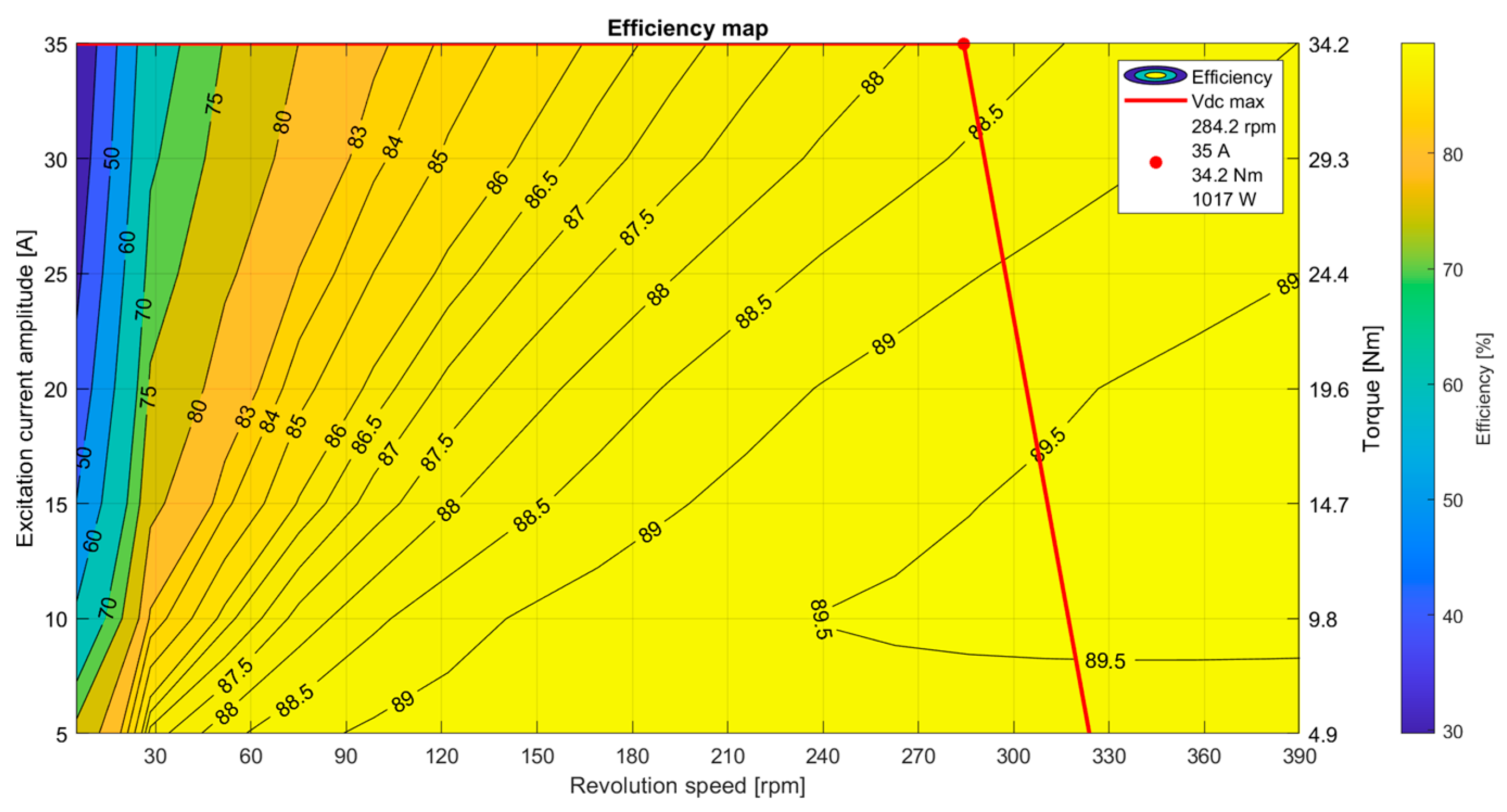
The efficiency map acquired from the simulation FEM model is shown in Figure 12. The limits of the efficiency map were determined by the DC voltage of the motor controller and the battery pack.
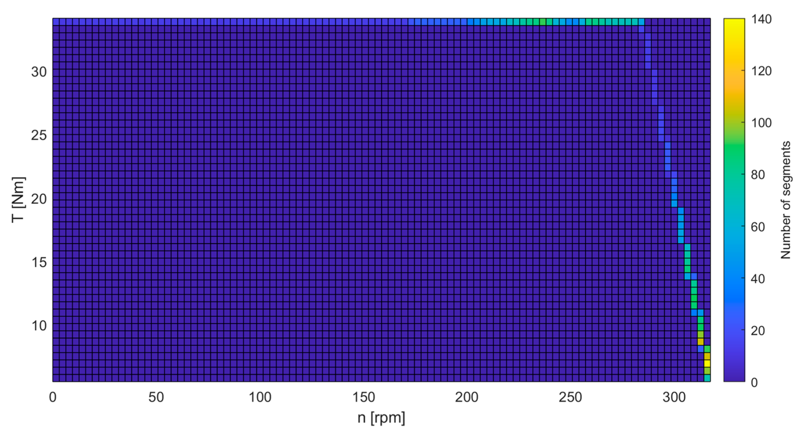
As the motor does not operate in the field-weakened range during the race, this range was not evaluated. The investigated driving strategy was optimized for TT-circuit Assen, which hosted the 2022 SEM competition. During the optimization, the 342 s lap was broken down into 0.01 s segments. In the duty cycle diagram, the colors indicate the number of 0.01 s segments where the drive was used at a given operating point. Since the drive is equipped with a free-wheel drive and no regenerative braking is applied, the free-wheel and braking operating points were not included here, so only 5110 segments of the duty cycle were considered. The driving strategy was optimized with the Max TRQ method, which is searching for places to apply torque and always applying the physically available maximum torque. The colors indicate how many of these 5110 segments were present at a given working point. The duty cycle associated with the impact system is shown in Figure 13.
4.3. The Operating Points of the Optimization
Based on the previously presented driving strategy, the optimization was performed by analyzing the losses at two main operating points described in Table 3.
One of the objectives of optimization is to minimize the energy loss of the motor. The power loss is determined in these speed–torque operating points and multiplied by the time weighting to determine the energy loss of the given operating point.
4.4. The Constraints of the Optimization
The constraints of optimization, beyond the upper and lower bounds of the design variables, are geometric constraints that do not allow us to consider infeasible motor designs. Only two linear and two non-linear geometric constraints were considered in the optimization because it was a goal to reduce the number of such constraints in the model when choosing the design variables and their limitations. In addition to these, there were two non-linear constraints to ensure that the drive system was capable of operating at a working point of 32 Nm and 270 rpm at a nominal clamp voltage of 48 V and a maximum excitation current amplitude of 35 A at the corner point of the electric motor. The linear constraints are
and
where is the number of poles. Equation (1) prevents the stator cuts from intersecting with the magnets, and Equation (2) prevents the rotor from intersecting with the stator. The nonlinear constraints are
and
where
is the number of parallel wires and and are the results of FEM simulations at the 32 Nm and 270 rpm operating points. The is coming from an iterative calculation which calculates the maximum number of parallel wires that can be inserted for a given slot geometry, wire diameter, number of turns and fill factor.
4.5. Results
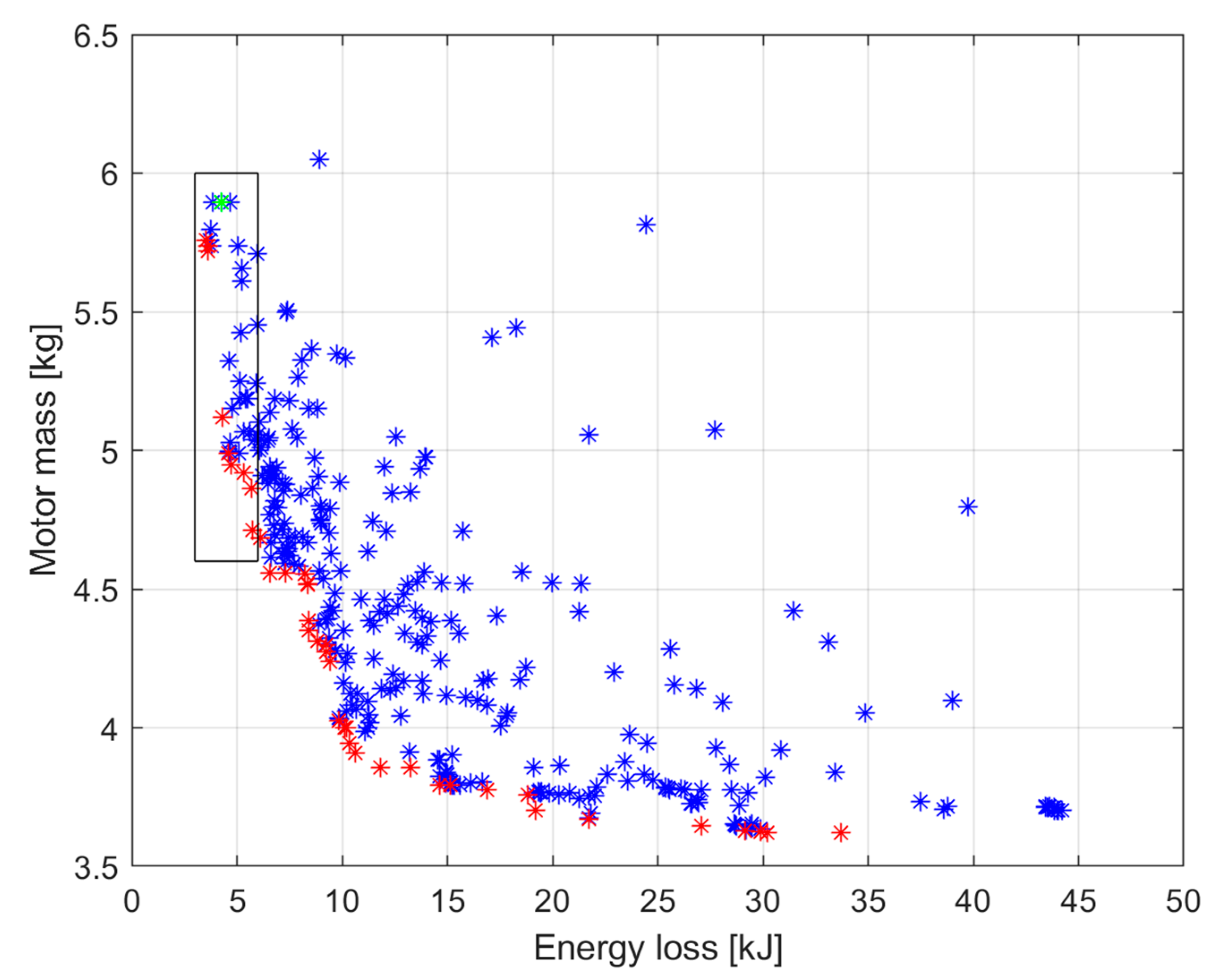
In the multi-objective optimization, a total of 588 motor designs were assessed, of which, only 544 required a full FEM simulation due to the kriging surrogate model. The kriging model only estimated the value of the loss calculation; the mass calculation was estimated from the geometry using the same method in all cases. The main reason why the kriging model was only able to replace 7.5% of the total evaluation was that the two objective functions were not properly balanced. During the optimization, the original motor outer diameter and length were specified as maximum limits for these design variables; the optimization algorithm was not able to test larger motors, which led to no significant improvement in terms of energy loss. Conversely, it was able to implement much smaller motors that were able to meet the constraints, and these were temporarily classified as non-dominated individuals given the uncertainty in the estimation. Since the algorithm considered both objective function values simultaneously and was able to produce much more favorable motor designs in terms of mass, the algorithm moved in this direction at the expense of energy loss. This also means that most of the individuals in the pareto front approximation had a much higher energy loss than the original motor, as can be seen in Figure 14.
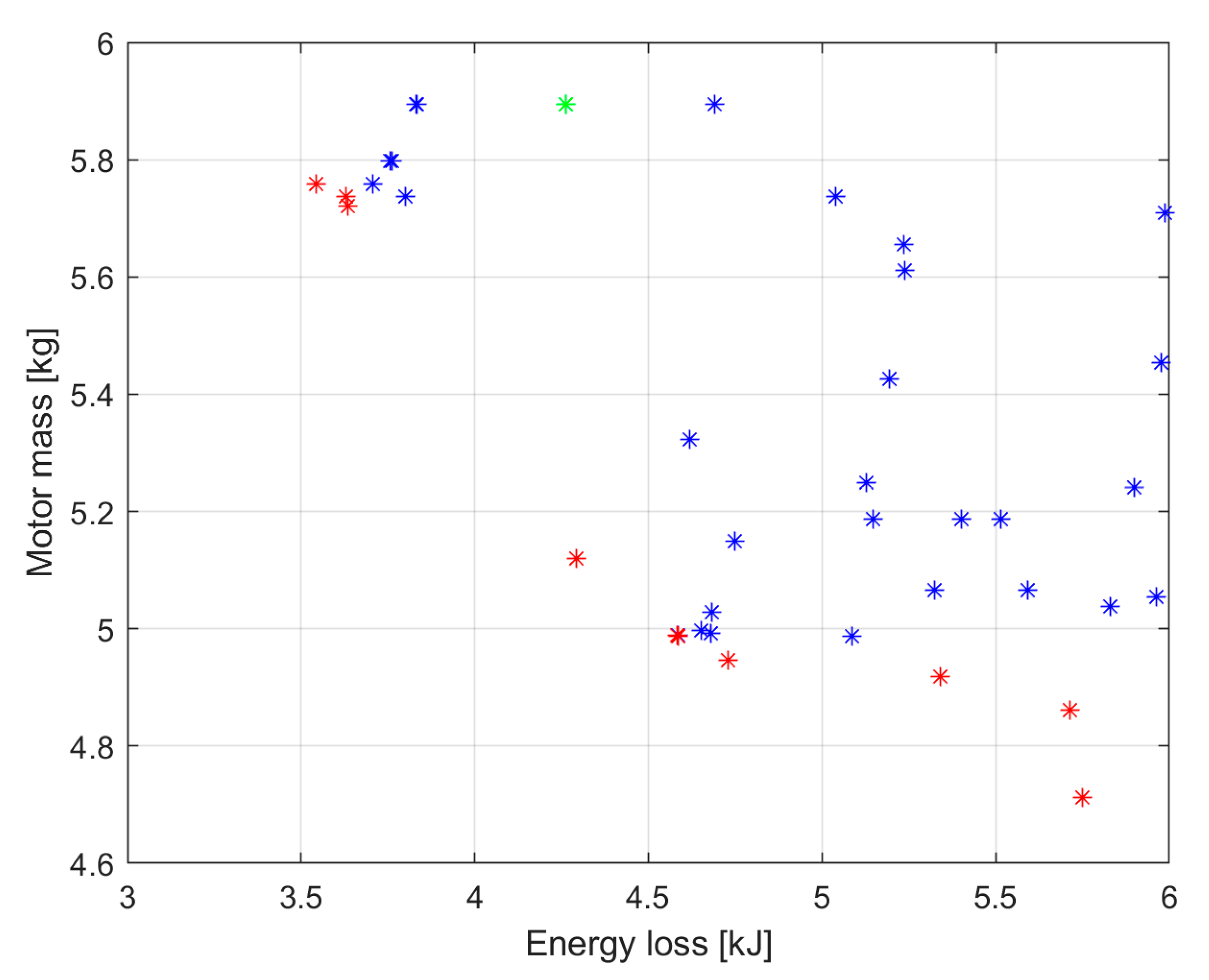
In Figure 14, the elements of the pareto front are marked in red, the non-dominated elements are marked in blue and the initial motor is marked in green. Although the optimization algorithm succeeded in creating a better motor in all aspects, this improvement was not significant, while at the same time, the lower mass motors produced disproportionately higher energy loss at the tested operating points. Figure 15 shows a zoomed-in image of the detail framed in Figure 14.
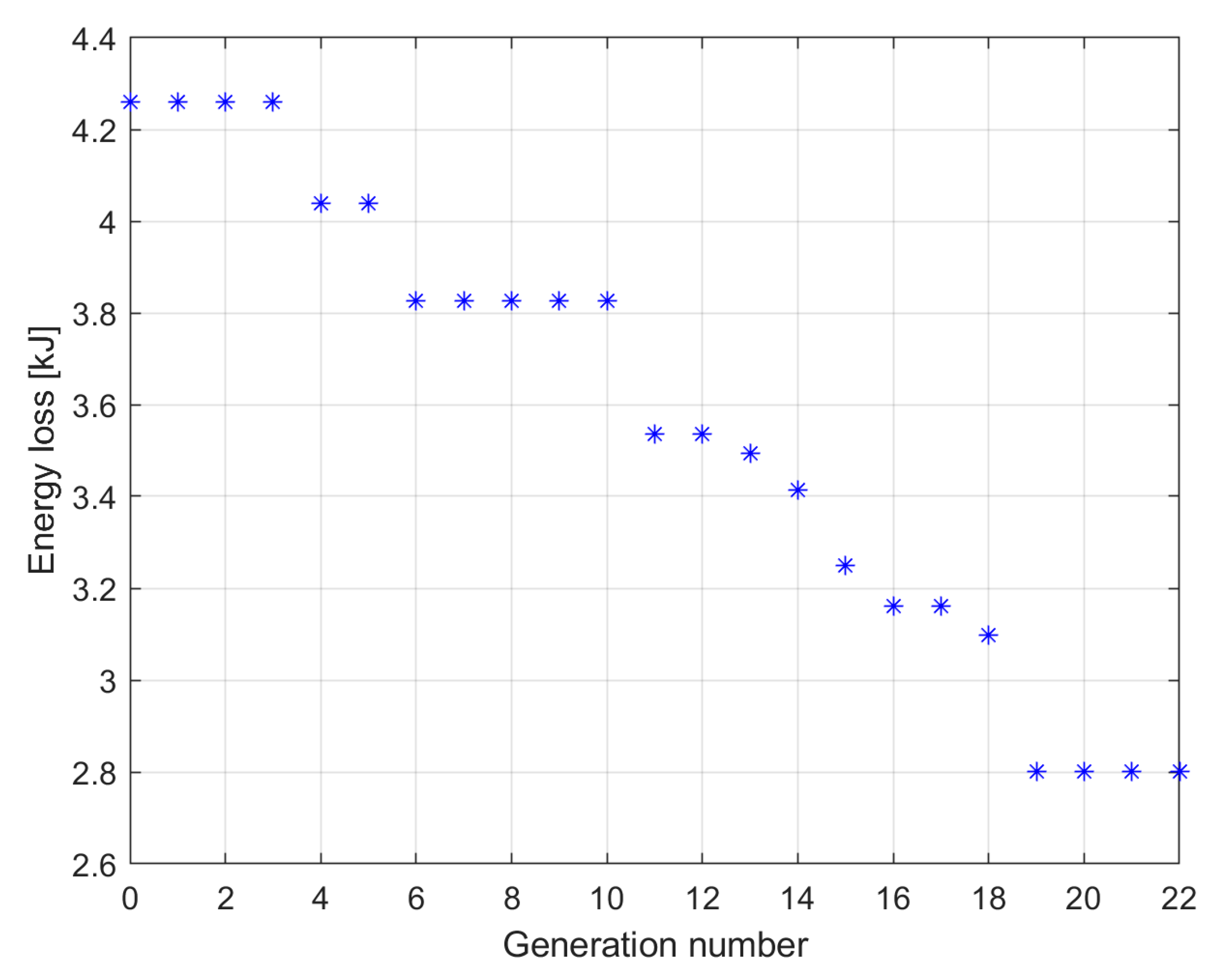
The results mentioned above demonstrate that a single-objective optimization that only focuses on loss energy can produce a better result in terms of loss energy. Because of the limitations imposed by the enclosure size, the mass cannot be larger than the initial mass of the SZEVOL. A total of 486 motor designs were considered in the single-objective optimization, of which only 273 required full FEM simulation due to the kriging surrogate model. In this case, the kriging was able to replace 43% of the evaluations. Figure 16 shows the motor with the lowest power loss per generation.
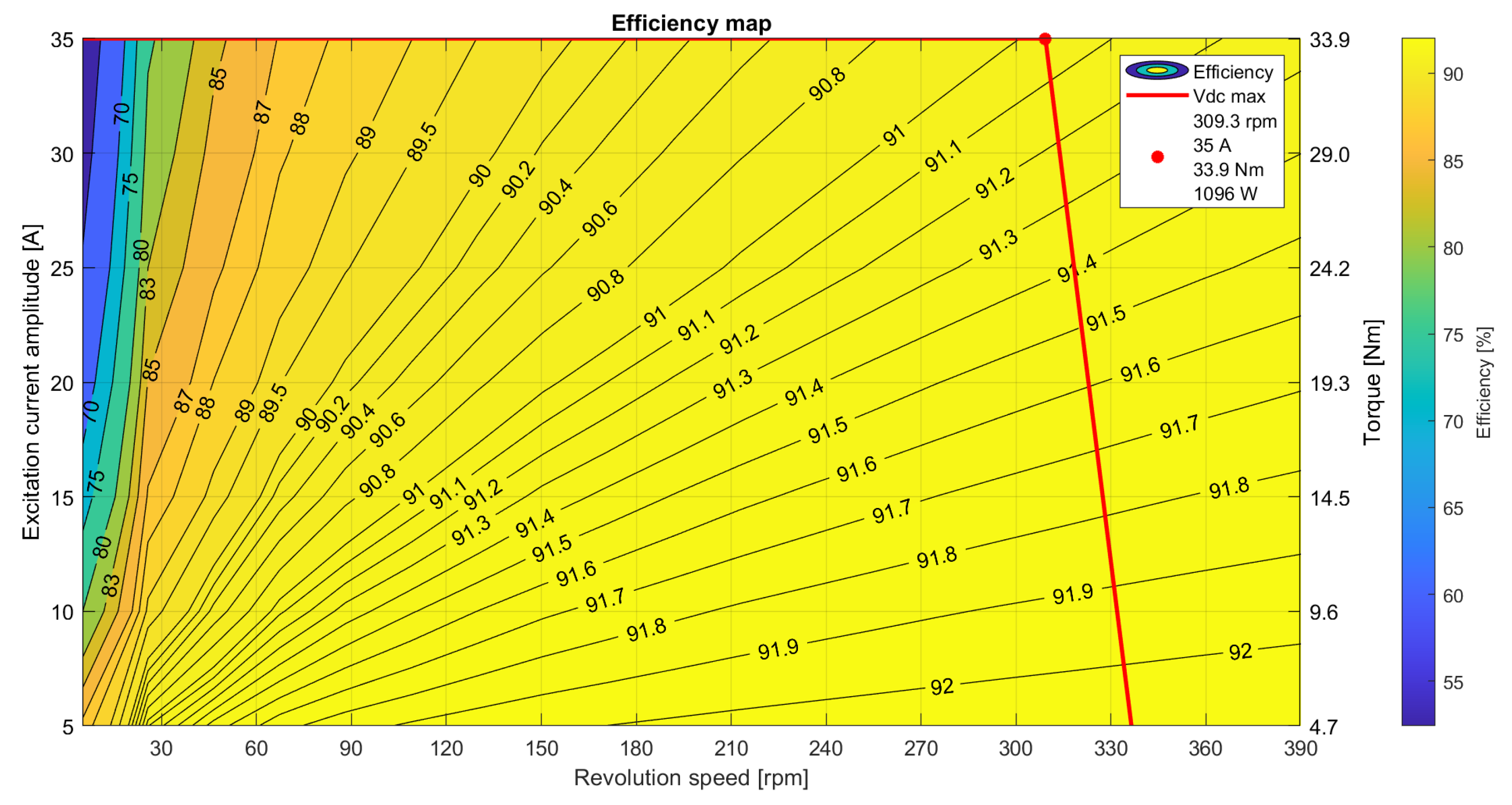
The resulting motor model produced 65.72% of the original motor’s energy loss at the analyzed predetermined operating points. The efficiency map of this motor is shown in Figure 17.
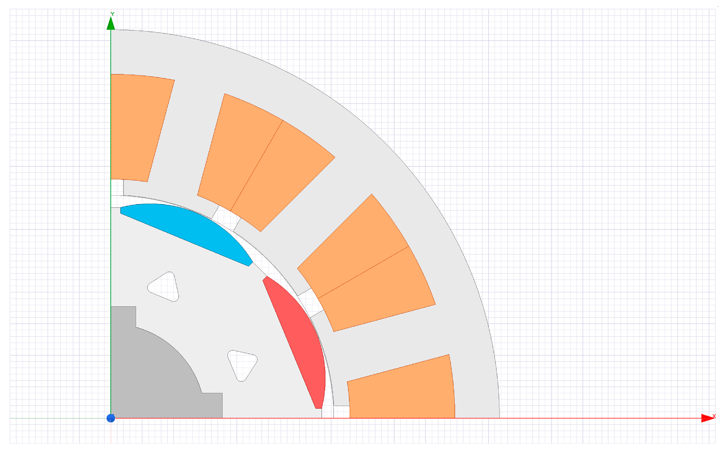
Compared to the SZEVOL motor, the optimized drive can operate with approximately 3% higher efficiency in the designated operating range. There were just slight modifications shown in terms of geometrical changes; the resulting geometry is shown in Figure 18.
The most significant changes were in the rotor cuts and tooth tangs. The effective wire cross-section increased by 20%, while the number of threads was reduced by 1, meaning that the phase resistance was also significantly reduced, which eventually reduced the ohmic losses.
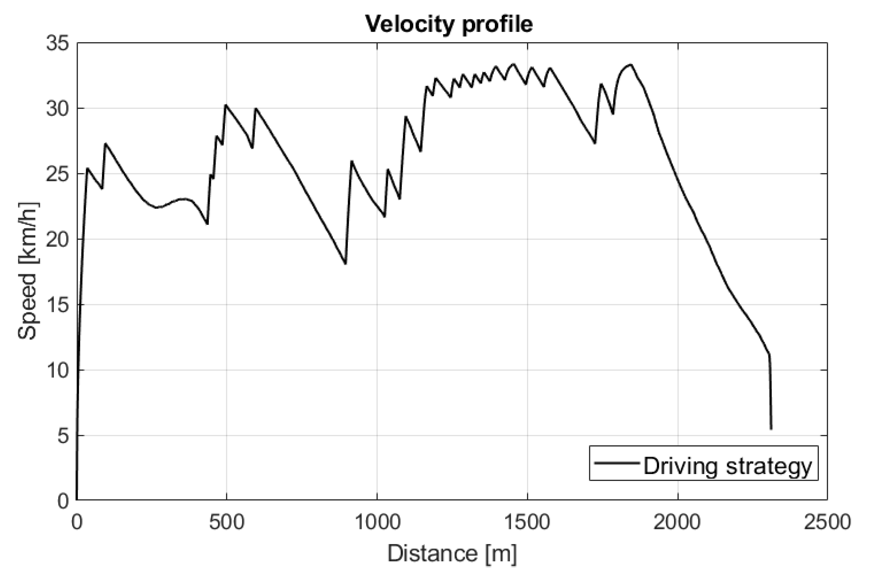
The resulting efficiency map of the optimized motor was compared to the reference by using the investigated velocity profile in the simulation environment. The optimized velocity profile for TT Circuit Assen is presented in Figure 19. It is important to highlight that this velocity profile was created via driving strategy optimization for the reference SZEVOL motor; therefore, it already used favorable operating points.
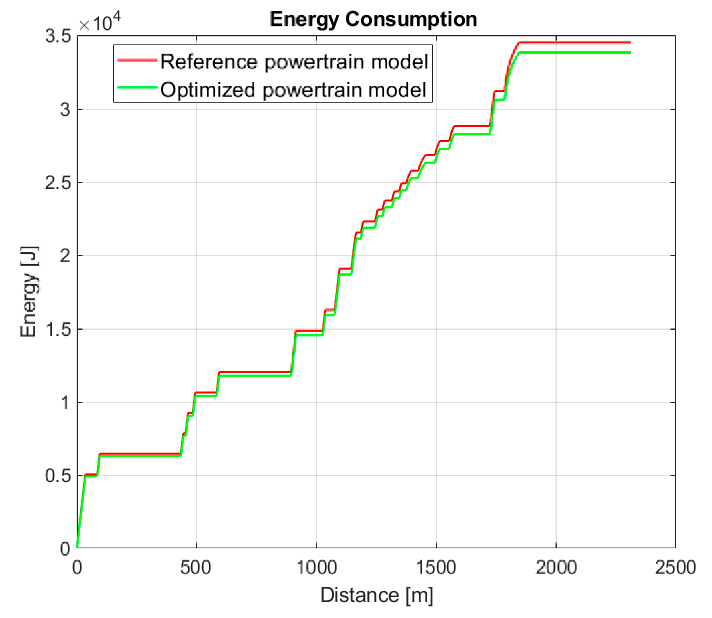
Powertrain models were created for the simulation model based on the FEM simulation results; these powertrain models represent the physical properties of the investigated drives. Two separate simulation cases were made, where the energy consumption levels of the drives implemented in the race vehicle were studied. The optimized powertrain could provide improvement compared to the reference result, reducing the energy consumption in one lap from 34.500 J to 33.830 J, which was an improvement of approximately 2%. The energy consumption curve of the investigated motors is shown in Figure 20. The motor optimization framework used discrete operating points to determine the objective of the optimization, although they were time weighted, but the real consumption savings could be properly investigated in complete vehicle simulations.
Both motors were tested with the same velocity profile (Figure 19) optimized for TT Circuit Assen for the experimental race vehicle equipped with the SZEVOL motor. The energy consumption of the SZEVOL-motor-powered race car during a lap is represented by the red line, while the green line represents the energy consumption of the same vehicle with an optimized motor design. While the improvement may not appear to be significant, it is important to note that the benchmark for comparison was the world record performance in the SEM race.
5. Conclusions
The validation of the optimization framework demonstrated the method’s suitability for improving electric motor design based on the determined operating points. The kriging surrogate model has the potential to considerably improve the performance of the framework under the condition that the optimization method is appropriately parameterized and constrained. This framework performs effectively in scenarios in which the drive system needs to operate at a specific duty cycle. The duty cycle is obtained from the driving strategy of an electric energy-efficient experimental vehicle, where the applied electric motor (SZEVOL) of the powertrain is under the scope of optimization.
In the case of the SZEVOL motor, the constraints’ formulation did not provide efficient optimization in terms of weight and loss reduction; therefore, single-objective optimization for loss reduction was chosen to improve the effectiveness of the drive system. Based on the results, it was possible to reduce losses by more than 30% at the operating points of the investigated driving strategy, which resulted in an increase in the drive system’s overall efficiency of more than 3% at the application-relevant operating points. This led to a 2% improvement in energy consumption according to the vehicle simulation; however, this improvement was achieved on a driving strategy, which was created with the vehicle using the reference SZEVOL motor. The process of the used driving strategy optimization was proposed in Ref. [13]. The achieved energy savings would be considerably greater with a redefined driving strategy specially made for the resulting electric motor.
The vehicle won the 2022 SEM competition, achieving a world record result with the SZEVOL motor. The 2% improvement in energy consumption should be evaluated within the context of this accomplishment. The original SZEVOL motor and the optimized motor were tested in a simulation environment, where the used vehicle model was identical except for the drive model, ensuring that measurement errors did not impact the comparison. Considering these outcomes, it may not be worthwhile to modify the existing motor for such a marginal increase in efficiency. However, the optimized motor is capable of operating at higher rotor speeds under a given nominal DC voltage, allowing it to reach the desired operating points even at a low battery voltage.
According to the results, it is also possible to increase the efficiency of the drive system mostly by changing the winding parameters. It may be more cost-effective to apply the optimization framework using the current motor geometry, as the design parameters only aim to modify the properties of winding. Rewinding the current motor based on the optimization results could also decrease the energy losses of the current system.
Author Contributions
Conceptualization, visualization G.I., writing—draft preparation G.I. and Z.P.; methodology, validation, and formal analysis, G.I., Z.P. and P.K.; supervision, project administration, and funding acquisition, Z.H. and F.F. All authors have read and agreed to the published version of the manuscript.
Funding
The research was supported by the European Union within the framework of the National Laboratory for Artificial Intelligence (RRF-2.3.1-21-2022-00004).
Data Availability Statement
Not applicable.
Acknowledgments
The authors also recognize the contribution of the SZEnergy Team, who contributed internal telemetry data, photos and support throughout the tests.
Conflicts of Interest
The authors declare no conflict of interest.
Nomenclature
| FEM | finite element method |
| GA | genetic algorithm |
| GSA | gravitational search algorithm |
| PMSM | permanent magnet synchronous machines |
| PSO | particle swarm optimization |
| SEM | Shell Eco-marathon |
| SZEVOL | the electric motor to be improved in the example application |
References
- Naik, S.; Bag, B.; Chandrasekaran, K. Comparative Analysis of Surface Mounted and Interior Permanent Magnet Synchronous Motor for Low Rating Power Application. J. Phys. Conf. Ser. 2021, 2070, 012119. [Google Scholar] [CrossRef]
- Istenes, G.; Horvath, Z. Multi-objective Optimization of Electric Motors with a Kriging Surrogate Model. In Proceedings of the IEEE 2022 22nd International Symposium on Electrical Apparatus and Technologies (SIELA), Bourgas, Bulgaria, 1–4 June 2022; pp. 1–4. [Google Scholar] [CrossRef]
- Elkholy, M.M.; Abd El-Hameed, M. Minimization of Starting Energy Loss of Three Phase Induction Motors Based on Particle Swarm Optimization and Neuro Fuzzy Network. Int. J. Power Electron. Drive Syst. 2016, 7, 1038–1048. [Google Scholar] [CrossRef]
- Das, S.; Mondal, S.; Saha, S.; Sarkar, C. A GSA Based Torque and Loss Optimisation of an Induction Motor. Int. J. Adv. Res. Electr. Electron. Instrum. Energy 2013, 26, 3717–3725. [Google Scholar]
- Bittner, F.; Hahn, I. Kriging-Assisted Multi-Objective Particle Swarm Optimization of Permanent Magnet Synchronous Machine for Hybrid and Electric Cars. In Proceedings of the 2013 International Electric Machines & Drives Conference, Chicago, IL, USA, 12–15 May 2013; pp. 15–22. [Google Scholar] [CrossRef]
- Sun, I.; Shi, Z.; Cai, Y.; Lei, G.; Guo, Y.; Zhu, J. Driving-Cycle-Oriented Design Optimization of a Permanent Magnet Hub Motor Drive System for a Four-Wheel-Drive Electric Vehicle. IEEE Trans. Transp. Electrif. 2020, 6, 1115–1125. [Google Scholar] [CrossRef]
- Sun, I.; Xu, N.; Yao, M. Sequential Subspace Optimization Design of a Dual Three-Phase Permanent Magnet Synchronous Hub Motor Based on NSGA III. IEEE Trans. Transp. Electrif. 2023, 9, 622–630. [Google Scholar] [CrossRef]
- Shi, Z.; Sun, X.; Cai, Y.; Yang, Z. Robust Design Optimization of a Five-Phase PM Hub Motor for Fault-Tolerant Operation Based on Taguchi Method. IEEE Trans. Energy Convers. 2020, 35, 2036–2044. [Google Scholar] [CrossRef]
- Kalyanmoy, D. Multi-Objective Optimization Using Evolutionary Algorithms; Indian Institute of Technology Kanpur: Kanpur, India, 2011; p. 24. [Google Scholar]
- Gong, W.; Duan, Q.; Li, J.; Wang, C.; Di, Z.; Ye, A.; Miao, C.; Dai, Y. Multiobjective Adaptive Surrogate Modeling-Based Optimization for Parameter Estimation of Large, Complex Geophysical Models. Water Resour. Res. 2016, 52, 1984–2008. [Google Scholar] [CrossRef] [Green Version]
- Maxwell 2D: ANSYS Maxwell tutorial on the 2004 PriusIPM Motor; Study of a Permanent Magnet Motor with MAXWELL 2D, ANSYS Maxwell. 2004, p. 95. Available online: https://www.academia.edu/35037357/Topic_Motor_Application_Note_Study_of_a_Permanent_Magnet_Motor_with_MAXWELL_2D_Example_of_the_2004_Prius_IPM_Motor (accessed on 15 May 2023).
- Ortiz García, G. Identificación de Sistemas Estructurales Histeréticos Usando Algoritmos de Optimización Multi-Objetivo; Universidad Nacional de Colombia, Industrial Automation: Manizales, Colombia, 2013; p. 112. [Google Scholar]
- Pusztai, Z.; Kőrös, P.; Szauter, F.; Friedler, F. Vehicle Model-Based Driving Strategy Optimization for Lightweight Vehicle. Energies 2022, 15, 3631. [Google Scholar] [CrossRef]
- Pusztai, Z.; Kőrös, P.; Szauter, F.; Friedler, F. Implementation of Optimized Regenerative Braking in Energy Efficient Driving Strategies. Energies 2023, 16, 2682. [Google Scholar] [CrossRef]
Figure 1.
An example of the Pareto front.

Figure 2.
The optimization framework.

Figure 3.
The FEM model of 2004 Prius IPM.

Figure 4.
The results of the Prius IPM FEM model: (a) the results of the technical report Ref. [11]; (b) the results of Ansys Maxwell.
Figure 4.
The results of the Prius IPM FEM model: (a) the results of the technical report Ref. [11]; (b) the results of Ansys Maxwell.

Figure 5.
FEM model of the SZEnergy motor.

Figure 6.
The results of the optimization: (a) the 3D results; (b) the 2D results.

Figure 7.
The final version of the SZEnergy motor.

Figure 8.
The manufactured SZEnergy motor.

Figure 9.
The efficiency map: (a) simulation; (b) measurements.

Figure 10.
The difference between the simulated and the measured efficiency.

Figure 11.
The cross-section of SZEVOL with the geometrical design variables.

Figure 12.
The simulated efficiency map of SZEVOL.

Figure 13.
The distribution of operating points in optimized driving strategy—SZEVOL driven at TT Circuit Assen.
Figure 13.
The distribution of operating points in optimized driving strategy—SZEVOL driven at TT Circuit Assen.

Figure 14.
The results of the multi-objective optimization.

Figure 15.
The results of the multi-objective optimization near SZEVOL.

Figure 16.
The results of the single-objective optimization.

Figure 17.
The efficiency map of the optimal motor model.

Figure 18.
The geometry of the optimized motor.

Figure 19.
Velocity profile for simulation comparison.

Figure 20.
Energy consumption of the vehicle using different powertrains in simulation environment.


Table 1.
Legend of the optimization framework.
| Parameters | Description |
|---|---|
| E | energy loss |
| Ep | previous energy loss |
| Ee | estimated energy loss |
| p | design variables |
| pp | previous design variables |
| t | time weight of operating point |
| Mr | required torque of operating point |
| n | rotation speed of operating point |
| M | calculated torque |
| I | required current amplitude |
| pi | additional variables |
| P | power loss |
Table 2.
The design variables.
| Name | Description | SZEVOL | Lower Limit | Upper Limit |
|---|---|---|---|---|
| x1 | Outer radius of the stator. | 61.75 mm | 50 mm | 61.75 mm |
| x2 | Thickness of the back-iron. | 7 mm | 5 mm | 10 mm |
| x3 | Depth of the slots. | 16.3 mm | 5 mm | 25 mm |
| x4 | Thickness of the tooth tangs. | 2.5 mm | 2 mm | 5 mm |
| x5 | Gap between the tooth tangs. | 1.5 mm | 1 mm | 10 mm |
| x6 | Thickness of the tooths. | 8 mm | 2 mm | 10 mm |
| x7 | Airgap. | 0.15 mm | 0.1 mm | 1 mm |
| x8 | Maximum thickness of the magnets. | 4.6 mm | 2 mm | 10 mm |
| x9 | Gap between the magnets. | 3 mm | 2 mm | 10 mm |
| x10 | Width of the rotor cuts. | 8 mm | 3 mm | 15 mm |
| x11 | Height of the rotor cuts. | 6.5 mm | 3 mm | 20 mm |
| x12 | Distance between the cuts and the origin of the axis. | 21.15 mm | 18.75 mm | 27.75 mm |
| x13 | Ratio of the magnet groove (x8/x13b). | 0.3577 | 0.1 | 0.9 |
| x14 | Number of turns. | 17 | 10 | 30 |
| x15 | Diameter of the wire. | 1.128 mm | 0.65 mm | 1.38 mm |
| x16 | Length of the motor. | 52.5 mm | 40 mm | 52.5 mm |
Table 3.
Operating points for optimization.
| Rotational Speed (rpm) | Required Torque (Nm) | Time Weighting (s) |
|---|---|---|
| 267 | 32 | 30.94 |
| 315 | 7 | 20.44 |
Disclaimer/Publisher’s Note: The statements, opinions and data contained in all publications are solely those of the individual author(s) and contributor(s) and not of MDPI and/or the editor(s). MDPI and/or the editor(s) disclaim responsibility for any injury to people or property resulting from any ideas, methods, instructions or products referred to in the content. |
© 2023 by the authors. Licensee MDPI, Basel, Switzerland. This article is an open access article distributed under the terms and conditions of the Creative Commons Attribution (CC BY) license (https://creativecommons.org/licenses/by/4.0/).
Share and Cite
MDPI and ACS Style
Istenes, G.; Pusztai, Z.; Kőrös, P.; Horváth, Z.; Friedler, F. Kriging-Assisted Multi-Objective Optimization Framework for Electric Motors Using Predetermined Driving Strategy. Energies 2023, 16, 4713. https://doi.org/10.3390/en16124713
AMA Style
Istenes G, Pusztai Z, Kőrös P, Horváth Z, Friedler F. Kriging-Assisted Multi-Objective Optimization Framework for Electric Motors Using Predetermined Driving Strategy. Energies. 2023; 16(12):4713. https://doi.org/10.3390/en16124713
Chicago/Turabian StyleIstenes, György, Zoltán Pusztai, Péter Kőrös, Zoltán Horváth, and Ferenc Friedler. 2023. "Kriging-Assisted Multi-Objective Optimization Framework for Electric Motors Using Predetermined Driving Strategy" Energies 16, no. 12: 4713. https://doi.org/10.3390/en16124713
Note that from the first issue of 2016, this journal uses article numbers instead of page numbers. See further details here.