1. Introduction
The main renewable energy sources (RES) for electricity generation are hydroelectric, wind, photovoltaic, solar, geothermal, and bioenergy. Increasing the share of renewable energy in power systems can lead to some challenges such as higher uncertainty due to wind and solar photovoltaic sources. One solution for a grid facing RES uncertainty is the use of energy storage systems, including pumped-storage hydropower (PSH), flywheels, batteries, compressed air, and power-to-gas (hydrogen) systems. Among them, PSHs are known as the “Green Battery” and provide about 90% of the storage capacity of Power Systems, worldwide [
1]. According to the International Energy Agency (IEA), electricity production from hydropower will rise from 4333 TWh in 2019 to 5722 TWh in 2030 [
2]. Moreover, it is predicted that the global installed capacity of PSH will increase from 158 GW in 2019 to 240 GW by 2030 [
3].
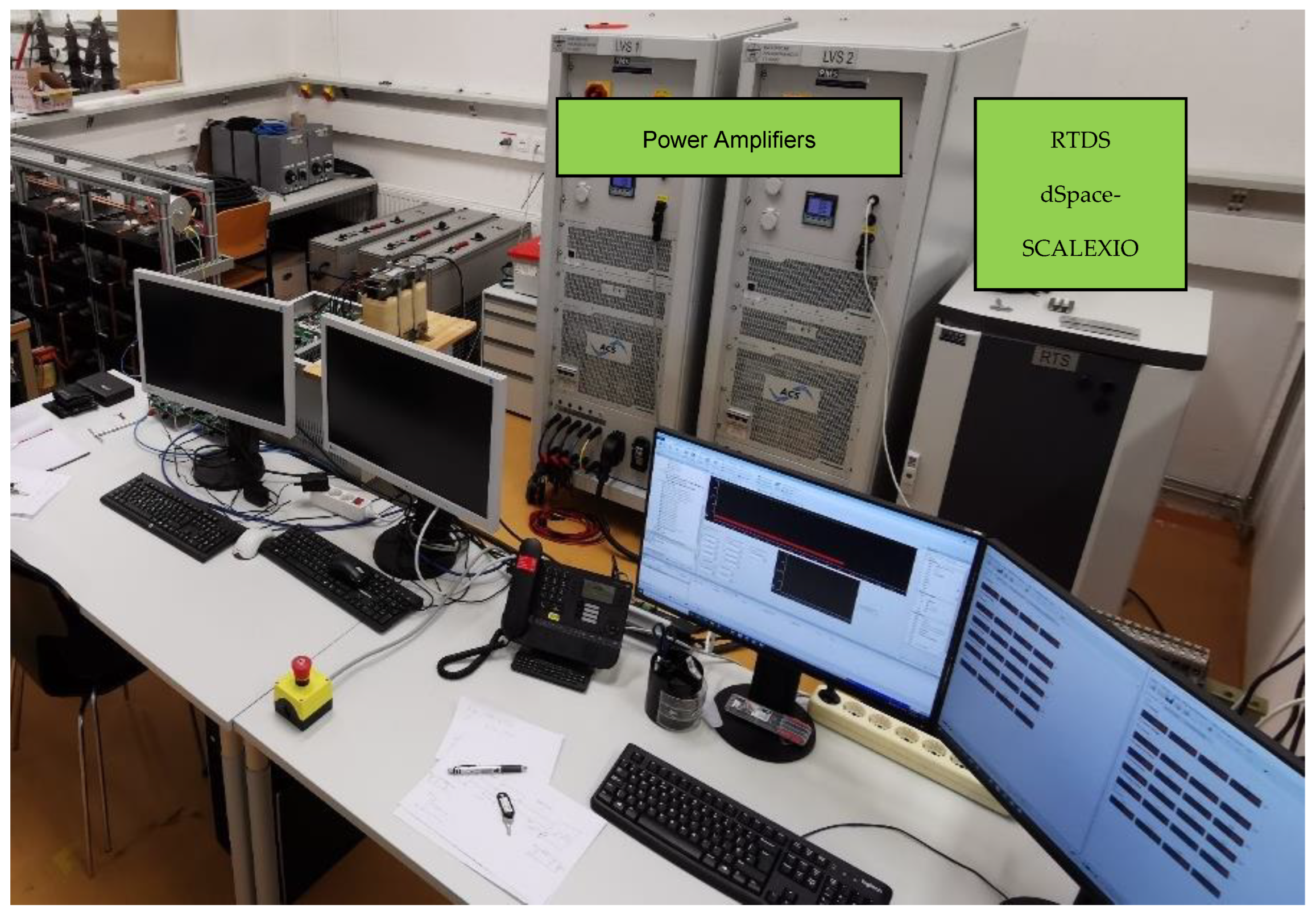
Due to the importance of PSHs in power systems and their vital role in future power systems, conducting research on the behavior of hydropower units in power systems with a new and powerful laboratory system as a real-time digital simulator (RTDS) is important. An RTDS is able to provide real-time results from the emulated power system and later on, it is possible to connect the RTDS to power amplifiers and emulate real electrical quantities from a specific part or specific parts of the simulated system.
There is a power hardware in the loop (PHIL) facility at the institute of electrical power systems at Graz University of Technology consisting of two power amplifiers (PAs) and a real-time digital simulator (RTDS) as depicted in
Figure 1 [
4]. A real-time digital simulator can be considered as the brain of a PHIL facility. An RTDS can analyze the input data and signals and then calculate, compute, and simulate the behavior and response of the objective systems, e.g., RES or grid. Next, it sends reference signals to the power amplifiers to emulate the electrical properties of the system under study.
Considering the significant benefits of an RTDS and a PHIL facility, researchers used them to conduct several studies and test their methods on these platforms. Several articles found an RTDS to be the right tool in order to compare and verify their simulation results with the RTDS results [
5,
6,
7,
8,
9,
10,
11,
12,
13,
14]. For example, Yang et al. proposed a co-simulation between FPGA and RTDS for the simulation of large power systems [
5]. In another work [
6], Krata et al. used an RTDS to test the voltage support to the grid from a battery energy storage system (BESS) combined with a PV system. In [
7], the authors developed a real-time benchmark model for integration studies of advanced energy conversion systems and they considered several technologies, including synchronous generators, PV, BESS, STATCOM, type-III and type-IV wind units, and simple hydropower units; however, they did not model the waterways and used a simplified model of the turbines. As a result, the transient and dynamic results of simple modelling can deviate from a real system. There are few works in the literature dealing with the simulation of hydropower plants in an RTDS. Some examples are given in [
8,
9,
10,
11,
12,
13,
14]. Most of these works ignore or use a simplified model of the waterways. Among these works, only two [
10,
11] consider an elastic water column model. Nonetheless, the configuration of the plant studied in [
11] is rather simplistic and comprises a single hydro pump-turbine unit, a penstock, a surge tank and a head-race tunnel. The configuration considered in our paper is much more complex and therefore computationally challenging to be simulated in an RTDS. The plant modelled in [
10] is the Dinorwig pumped-storage hydropower plant. The plant is equipped with six reversible pump-turbines and has a low-pressure tunnel, a surge tank, and a high-pressure tunnel, which ends in a manifold that distributes the water between the six hydro units [
15]. The configuration of the plant has the same degree of complexity as the one simulated in this paper. However, in [
10], as well as in [
8,
9,
11,
12,
13,
14], simplified models of the turbine typically used in power system studies are used.
One significant hydraulic part of a pumped-storage hydropower plant is a waterway including water tunnels, surge tank, and penstocks, since they play an integral role in the transient and dynamic behavior of hydropower plants. In [
16], the authors evaluated different waterway modelling techniques for RTDS applications. In this paper, the three main techniques for modelling a waterway, including the rigid model [
17], the lumped parameter approach [
18], and the polynomial approximation of a hyperbolic function [
19], were modeled, simulated, tested, and discussed. According to their evaluation, modelling a waterway based on the polynomial approximation of a hyperbolic function can provide an acceptable result.
The authors in [
20] evaluated three different methodologies for modelling Francis a pump-turbine for RTDS applications. In this paper, the three main methods for modelling a Francis pump-turbine, including the proposed IEEE model [
21], the linearized model around the operating point [
22], and the hill chart-based interpolation model [
23] were modeled, simulated, tested, and discussed. Based on the results from [
19], the hill chart-based interpolation model is the most suitable model that can accurately represent the turbine model at different operation points.
In the literature, the existing hydraulic machine models, such as turbines, rarely contain the internal dynamic reaction of such devices. As a result, turbine models are focused on determining the static relationship between the key hydraulic variables (net head, flow, wicket gate position or guide vane opening, and rotating speed) and the efficiency of the turbine for each operating point. This information is graphically presented in the well-known turbine hill charts. For instance, the hill chart, defined as a function of unit speed n
11 and unit flow q
11, is used in [
24] to analyze the stability of a run-of-river power plant with a water level control rather than the conventional frequency control. Clearly, a point cloud that has been mathematically interpolated is used to introduce the hill charts in the dynamic model. These curves are sometimes linearized so that the resulting linear equations can be easily incorporated into the hydroelectric power plant’s mathematical model. This approach is very useful for analyzing small disturbance occurrences in a power plant, as shown in [
25,
26].
Sadly, many times there is no particular information available concerning the turbine. In such cases, the universal expressions suggested in [
21] are widely used. The works [
15,
27] contain a couple of examples on how to use these expressions. Furthermore, in some circumstances, a first order transfer function is used to incorporate governor movement dynamics into the model [
28]. The main objective and contribution of this paper is to evaluate the capability of an RTDS to accurately emulate the hydraulic, mechanical, and electrical transients taking place in a pumped-storage hydropower plant with a complex configuration.
The following sections briefly discuss different modelling techniques for the Francis turbine and waterway. Then, a sample power system including a complex hydropower plant with four units containing 4 Francis turbines, one long headrace tunnel, a surge tank, two common penstocks, and four short penstocks is modeled. Finally, the capability of a real-time digital simulator to provide results for this system is evaluated by presenting and discussing the RTDS results for different situations.
2. Design Methodology
2.1. Turbine Models
Here, three well-known modeling techniques of the Francis turbine are presented:
The IEEE model presented in [
21].
The linearized model around an operating point [
22].
The hill chart-based interpolation model [
23].
The IEEE model calculates the dynamic pressure head of the turbine based on the input flow into the turbine and the guide vane opening (gvo) position:
where
h is the dynamic pressure head of the turbine,
q is the input flow of the turbine,
gvo is the guide vane opening position,
t is the torque of the turbine, and
η is the turbine’s efficiency.
In the linearized model, two operation points (steady state operation point and second arbitrary operation point) of the turbine from the hill-chart characteristic should be selected and then the following equations can represent the behavior of the turbine between the two selected points [
17]:
where
Δq,
Δh, Δn, Δgvo, and
Δt are the flow change, change in the dynamic pressure head, speed change, change in the guide vane opening position, and change in torque, respectively. The partial derivatives of the flow and torque over the pressure head, speed, and guide vane opening are calculated based on the data of the two selected operation points, in which the first point was selected close to the rated steady state condition and the second point was selected with 0.1 pu less power than the first one. More information is presented in [
22].
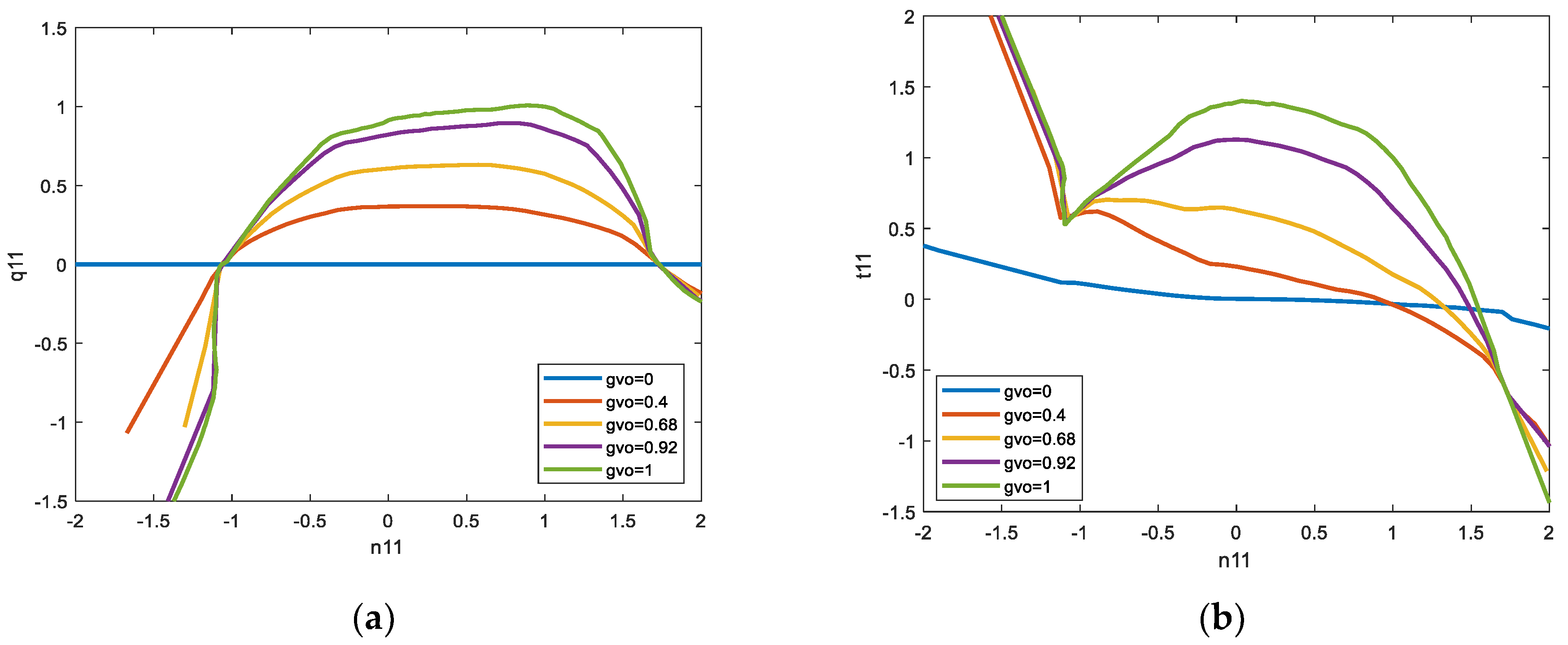
The hill chart is a different modeling approach for the Francis pump-turbine. Based on the experimental findings of the pump-turbine under various test settings, hill charts are prepared. The q
11-n
11 and t
11-n
11 basic hill chart diagrams display a set of values for the unit flow, unit speed, unit torque, and unit speed for different guide vane opening destinations.
Figure 2 demonstrates the general hill chart curves for a Francis pump-turbine. With the help of a hill chart, it is possible to find other values for different operation points. To use the hill charts, it is recommended to consider the polar coordinate as proposed in [
29] and as a result, plots such as
Figure 3 can be applied to simulate the behavior of the Francis pump-turbine.
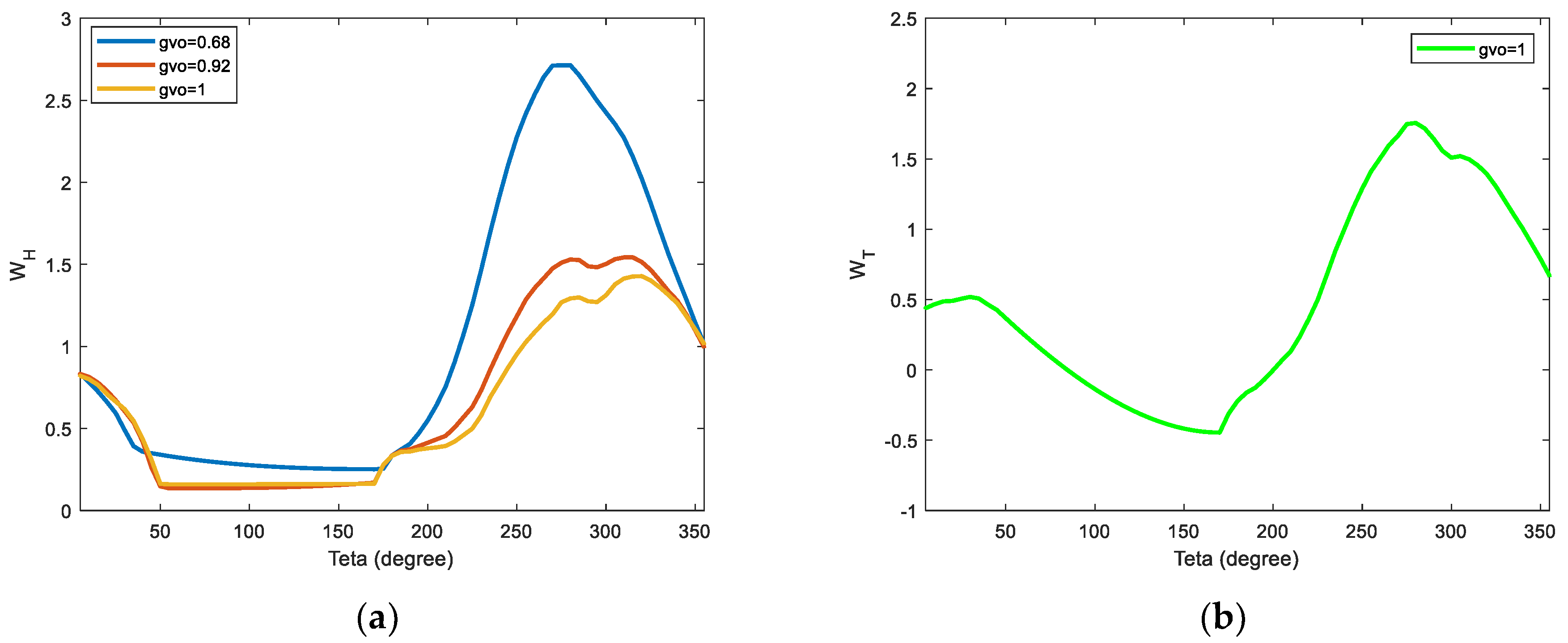
The following formulas are implemented to transfer the measured hill chart data to the polar frame and vice versa:
where
θ is the polar angle of the operation point with the unit flow of
q11 and unit speed of
n11,
Wh(
θ) is the parameter for the dynamic pressure head of the turbine, and
Wt(
θ) is the parameter used to calculate the output torque of the turbine in the operation point.
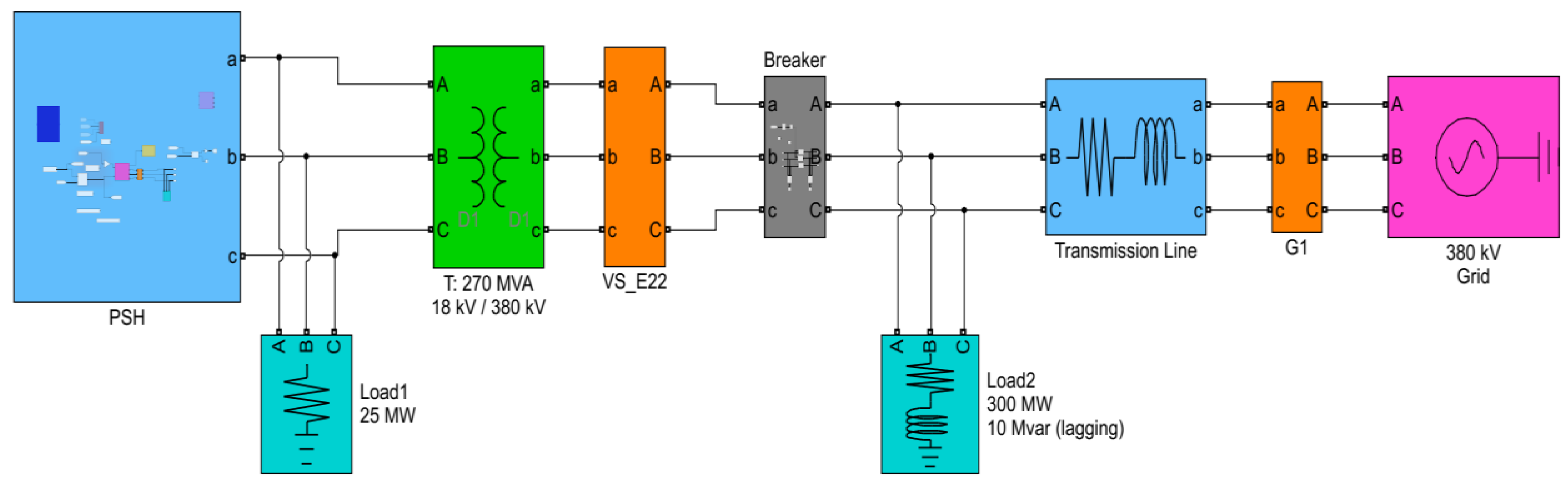
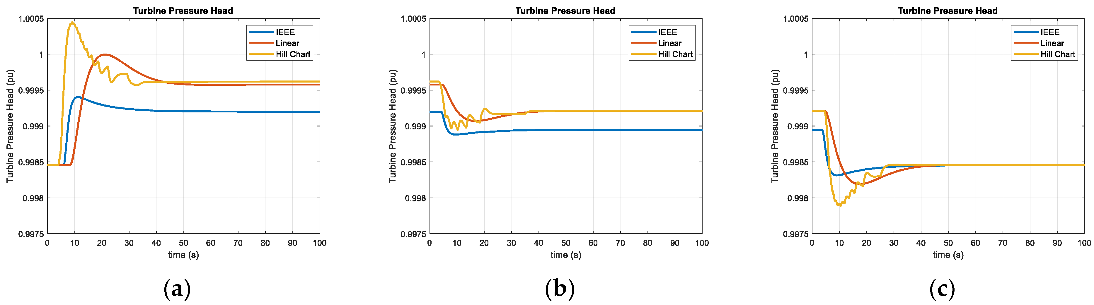
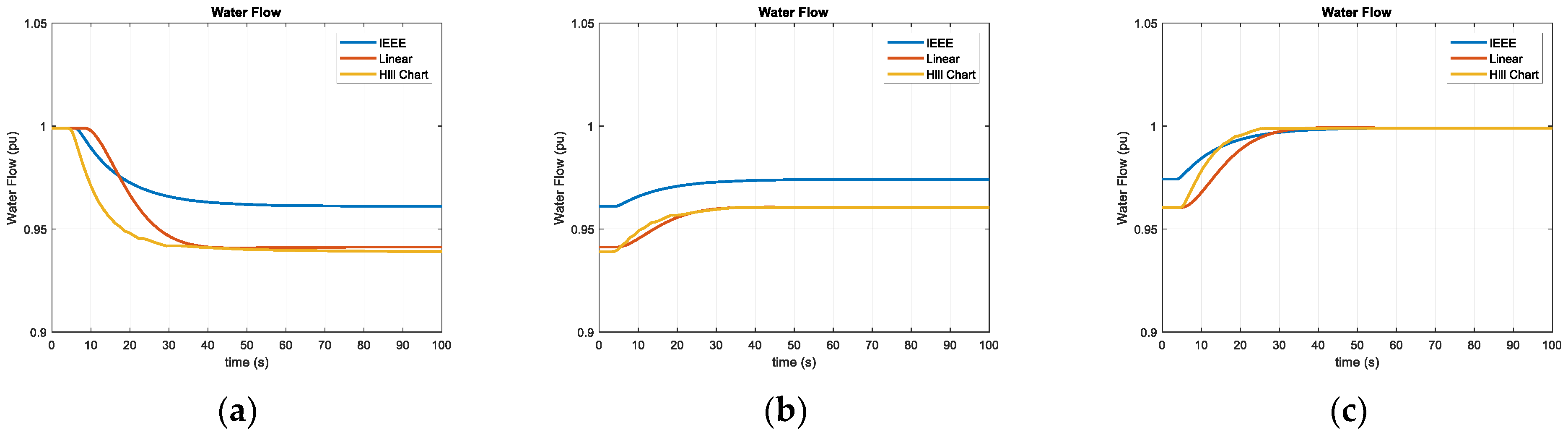
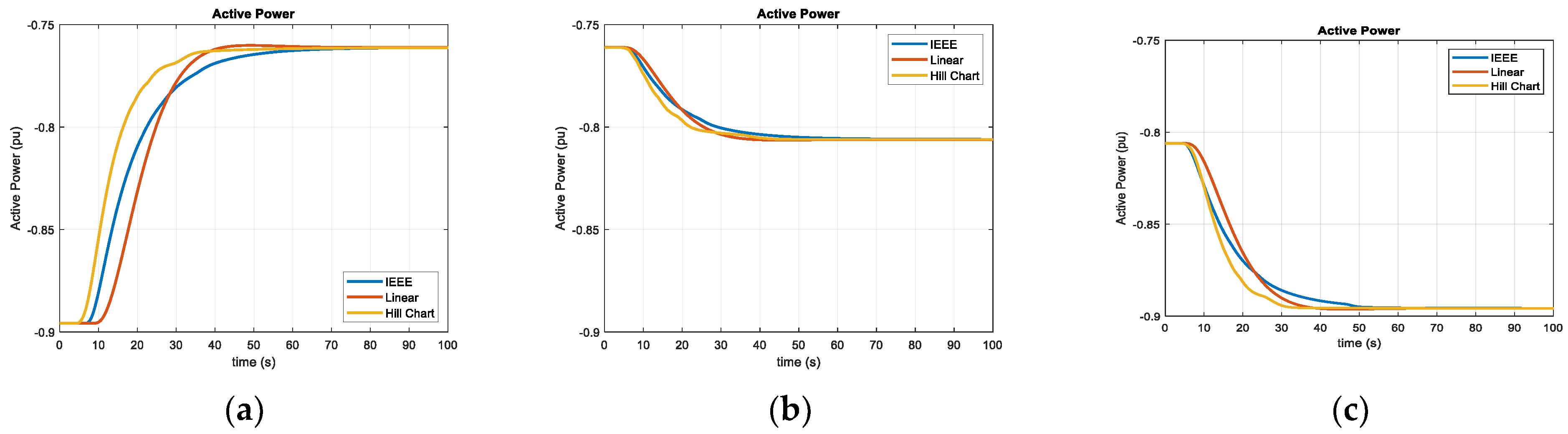
The authors in [
20] studied the RTDS results for different turbine modeling techniques. The sample power system for this study is depicted in
Figure 4 and the details of the system are presented in [
20]. Here, some of the results are reproduced in
Figure 5,
Figure 6 and
Figure 7.
According to the results of [
20], the most accurate model to represent the transient and steady state behaviors of the Francis pump-turbine is the hill chart-based model; however, it has the highest calculation burden in the RTDS and the experimental hill chart data for the turbine are not always available. The IEEE model is able to show the steady state behavior if the efficiency factor is updated for every new operation point; however, the IEEE and linearized models are not suitable for presenting the transient behavior of a turbine. The linearized model also needs updated coefficients for a more acceptable result for the steady state condition.
2.2. Waterway Models—Headrace Tunnel and Penstocks
In a pumped-storage hydropower plant with a large penstock or water tunnel, it is common to use a surge tank to reduce the water hammer effect or pressure wave in the waterway system. Therefore, in this section, modelling a penstock and surge tank is presented.
In general, there are two types of waterway modeling: one that is non-elastic (rigid) and ignores the compressibility of water and the elasticity of the waterway and is simple to implement; and the other one, which considers the compressibility of water and the elastic behavior of the waterway and is much more complicated than the rigid type, especially when modeling units with common waterways. The elastic water column dynamics in an ideal waterway without losses, including a water tunnel and a separated (single) penstock, can be formulated as follows [
17]:
Hc: Dynamic head at the junction of tunnel-penstock(s)
Qc: Dynamic flow at the junction of tunnel-penstock(s)
Hd: Dynamic head established by pump-turbine unit(s)
Qd: Dynamic flow established by pump-turbine unit(s)
Hs: Total available static head (Hs1 + Hs2)
Hs1: Static head between upper reservoir water surface and tunnel-penstock(s) junction
Hs2: Static head between tunnel-penstock(s) junction and lower reservoir water surface
Tet, Zht: Elastic time and hydraulic impedance of the tunnel part of waterway
Tep, Zhp: Elastic time and hydraulic impedance of the penstock
Te: Elastic time of the conduit, penstock, water tunnel (s)
L: Length of the conduit, penstock, water tunnel (m)
a: Water pressure wave velocity (m/s)
Tw: Water starting time of the conduit, penstock, water tunnel (s)
A: Cross section area of the conduit, penstock, water tunnel (m2)
Qb: The base water flow/discharge (m3/s)
ag: The gravitation acceleration (9.81 m/s2)
Hb: The base head is usually equal to the total available static head (m)
Considering several PSH units with a common waterway, the water flow (discharge) in a common waterway (tunnel) is the sum of the water discharge in all penstocks connected to the common tunnel. For example, if N units have a common water tunnel, the dynamic discharge in the
ith penstock and dynamic discharge in the common water tunnel can be calculated as follows [
17]:
Qc: Dynamic flow at the junction of the common tunnel and connected penstocks
Hdi: Dynamic head established by the ith pump-turbine unit
Qdi: Dynamic flow established by the ith pump-turbine unit
Hs: Total available static head
Tet, Zht: Elastic time and hydraulic impedance of the common tunnel
Tepi, Zhpi: Elastic time and hydraulic impedance of the ith penstock
The mass and momentum conservation equations define the relationship between the flow and pressure in the pressured conduits [
30]. These equations combine to generate a system of partial differential equations that can be represented as a hyperbolic tangent function in the frequency domain [
21,
31]. It can be challenging to implement such a transfer function in numerical simulation tools or real-time digital simulators. Several techniques for solving these equations have been proposed in the literature. The easiest approach is to ignore the conduit’s elasticity and water compressibility, resulting in a single first-order differential equation. Waterway models based on this simple approach are referred as either non-elastic or rigid water column models in the literature [
32]. In some circumstances, non-elastic water column models produce satisfactory results [
23]. According to [
33], when the Allievi parameter is greater than one, the elastic effects should not be ignored. One of the most generally used methods for solving the above-mentioned system of partial differential equations is to divide the conduit into segments and assign a proportional fraction of the conduit’s losses, inertia, and elasticity to each segment [
34]. A single first-order differential equation is applied within each segment to examine the conduit’s losses and inertia, while another one is utilized between each two segments to consider the conduit’s elasticity and water compressibility [
35]. Preliminary research may be required to determine the number of segments required to appropriately represent the conduit’s performance [
36]. The distribution of losses, inertia, and elasticity among the segments is determined by assessing the boundary conditions [
18].
The discharge equation for the rigid model of a single penstock by assuming that
Qc =
Qd in Equation (11) can be written as follows:
Twt: Water starting time of the tunnel part of waterway, Twt = Tet Zht
Twp: Water starting time of the penstock part of waterway, Twp = Tep Zhp
The common penstock and waterway are modelled based on the first-order polynomial approximation of the hyperbolic by considering the polynomial approximation of the tanh function as presented in Equation (20) [
19]:
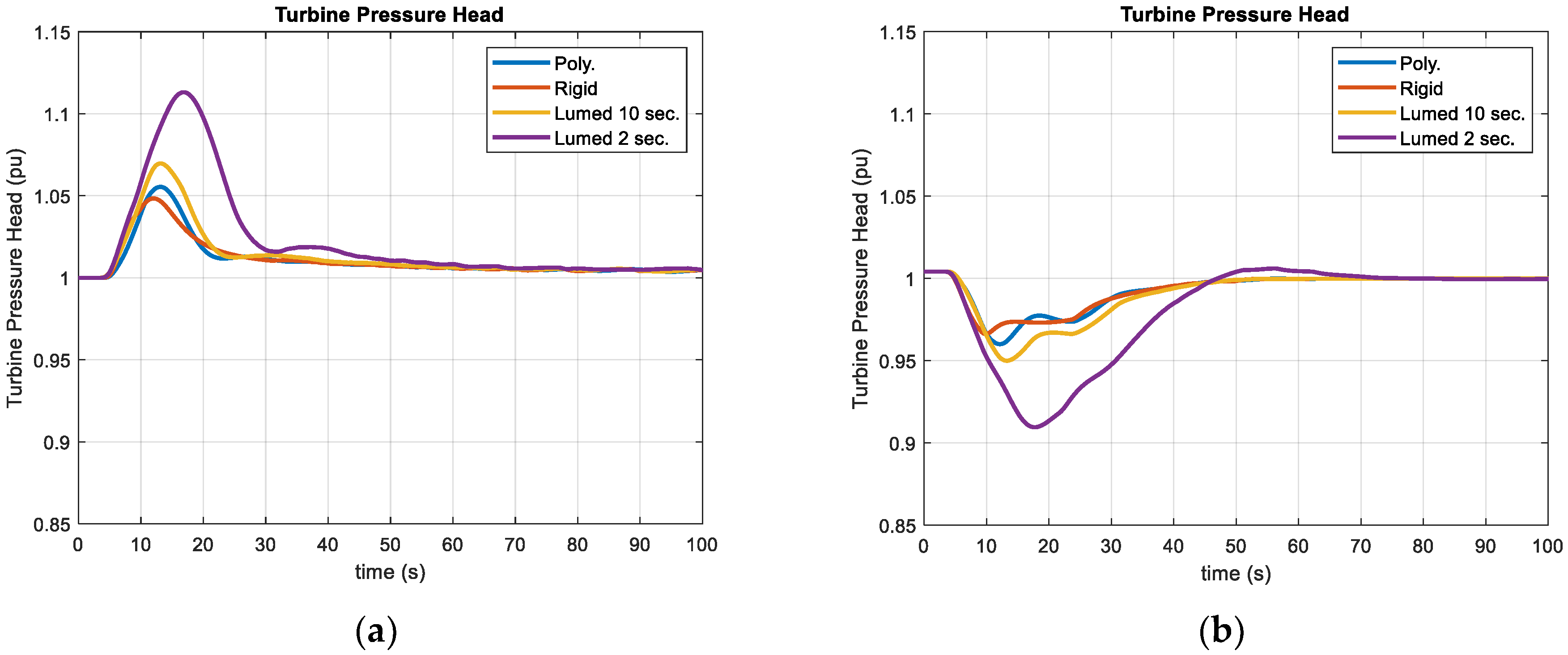
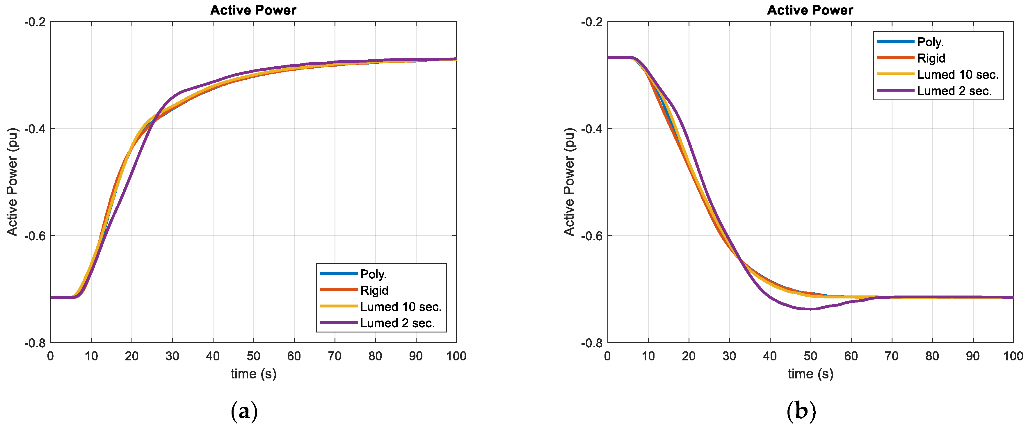
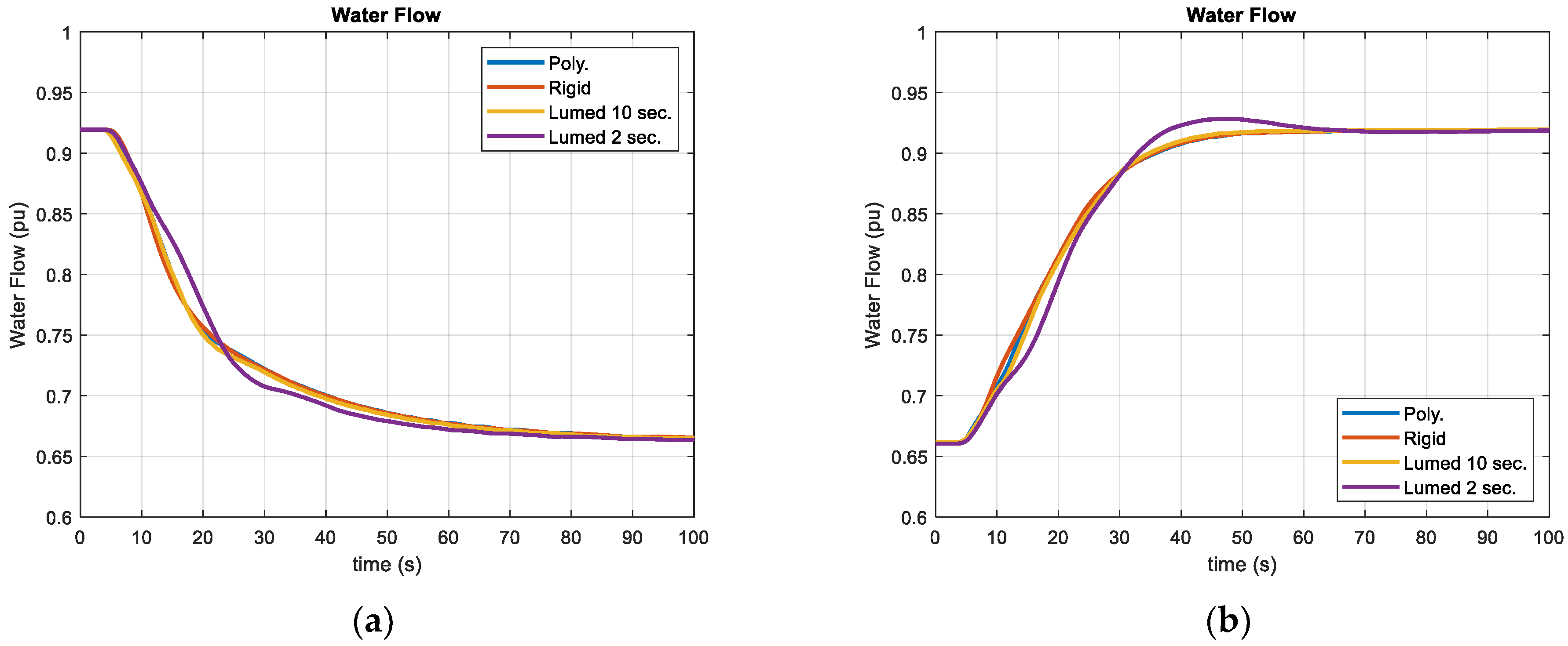
In [
16], the RTDS results for the three main modeling methodologies for a waterway, including the rigid model, the polynomial approximation of a hyperbolic function, and the lumped parameter approach (with 2 sections and 10 sections of the conduit) on a simple power system with one hydropower unit as depicted in
Figure 4 are compared. The following diagrams,
Figure 8,
Figure 9 and
Figure 10, present the results from [
16]:
According to [
16], the correct model of a penstock can be achieved either by the lumped parameter approach with a high number of sections or by a polynomial approximation of the hyperbolic function method; however, for a long penstock, the high number of sections in the lumped parameter approach can raise the computational burden on an RTDS in addition to the higher complexity and order of the state space equations for the whole system in the RTDS.
2.3. Waterway Model—Surge Tank
One of the main problems that hydroelectric power plants have when they are operating is managing the pressure in the hydraulic conduits, especially in the penstock. Thus, the necessary kinetic energy must be supplied to the water in the conduit during the start-up operations, while this energy must be absorbed in the event of a plant shutdown, whether accidental or programmed. In both cases, such changes in the water velocity result in sudden variations in water pressure in the pipeline known as a water hammer. These pressure variations do not only occur during the aforementioned maneuvers. During the normal operation of the plant, the changes caused by the action of the distributor on the flow rate as a result of the regulation services carried out by the plant are translated into changes in the pressure of the fluid. These pressure variations result in a loss of power quality and possible wear due to the fatigue of different components such as the penstock itself, the runner, or the wicket gates.
A water hammer is closely related to the length of the penstock that feeds the turbine. The water contained in a very long penstock significant inertia. If the plant is located sufficiently far from the intake, i.e., the upstream reservoir, the water hammer acquires significant values, which not only affects the dynamic response of the plant as described above but also has implications for the material used to build the pipe, whose modulus of elasticity and thickness will be high. This issue has a very important repercussion on the plant’s budget. One of the means used to minimize a water hammer is the location of a surge tank as close as possible to the turbine. In this way, the water hammer is confined to the penstock between the turbine and the surge tank with very low values, while the pipe between the surge tank and the reservoir is exempt from such pressure variations. The variations In the water level In the surge tank make It possible to provide or dissipate the required kinetic energy for the water in the conduit between the reservoir and surge tank, usually called the headrace tunnel.
The most common design for a surge tank is usually a constant, circular cross section. Sometimes a more complex geometry is used, introducing changes in the section of the surge tank, especially at its lower and upper ends, in order to reduce its height. In these cases, the construction process of such an element can be very expensive. In this study, a surge tank with a constant circular cross section of 491 m2 has been introduced in the hydropower plant model.
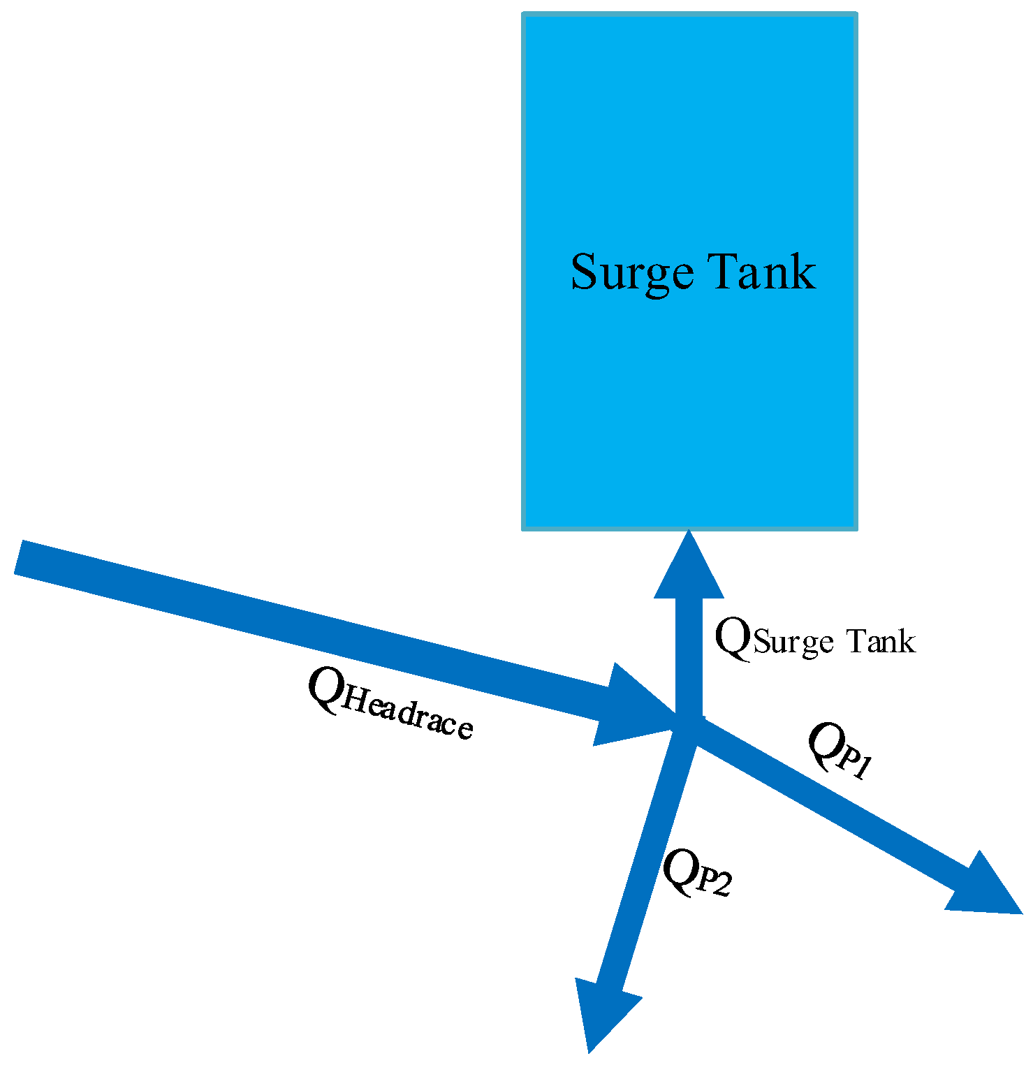
For the surge tank in
Figure 11, it is possible to calculate the water flow into this ideal surge tank based on the area of the surge tank and rate of change of the surge tank water level as shown in the following formula:
QSurge Tank: Water flow/discharge into the surge tank (m3/s)
ASurge Tank: Cross-section area of the surge tank (m2)
HSurge Tank: Water level in the surge tank (m)
QHeadrace: Water flow/discharge coming from the headrace tunnel to the surge tank (m3/s)
QP1: Water flow/discharge into the penstock 1 (m3/s)
QP2: Water flow/discharge into the penstock 2 (m3/s)
TSurge Tank: The time constant (storage constant) of the surge tank (s)
Qb: The base water flow/discharge (m3/s)
Hb: The base head, usually equals to the total available static head (m)
Modelling a surge tank, taking losses into account, is presented in [
23].
2.4. System under Study
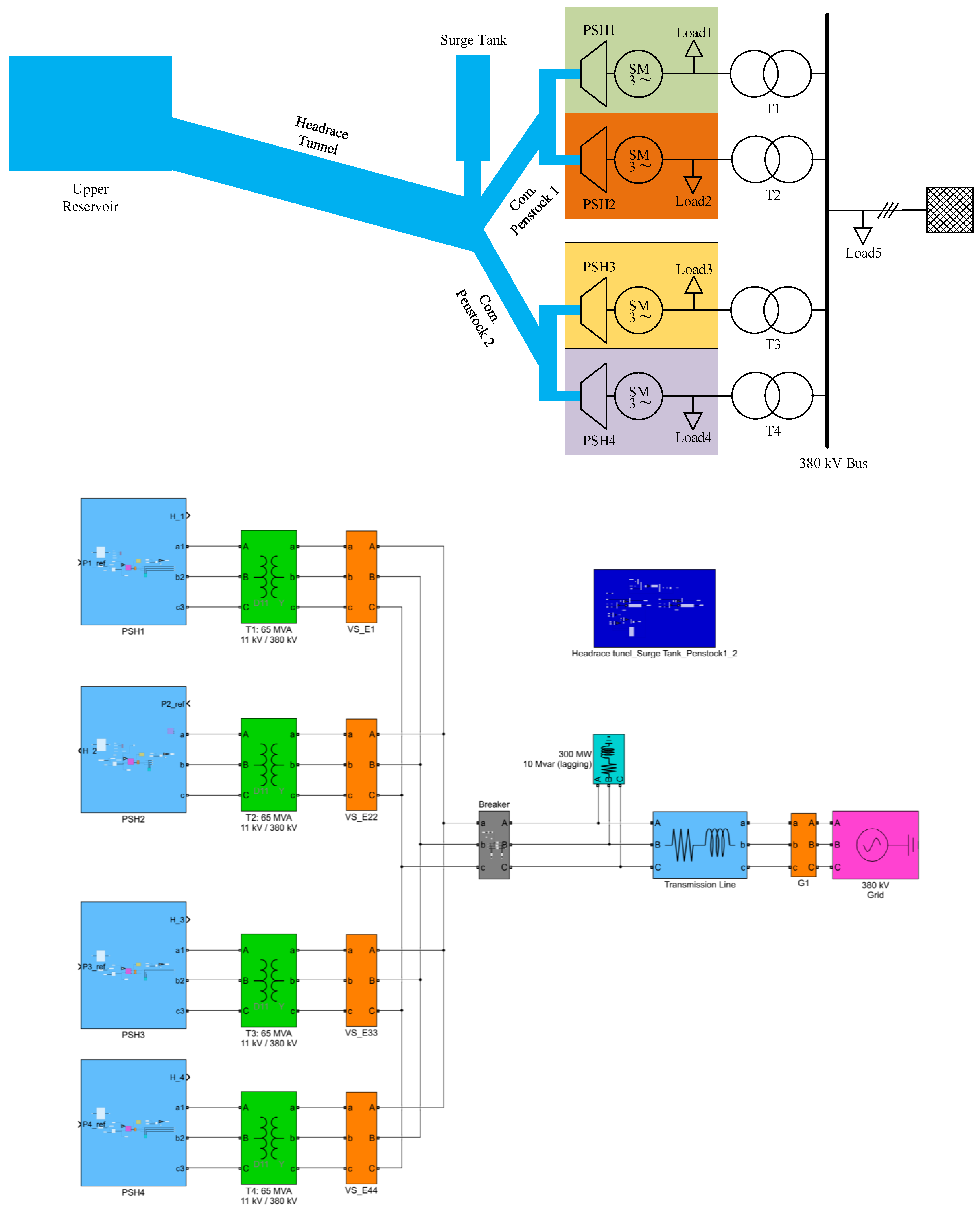
As mentioned in the above section, the brain of a PHIL laboratory is the RTDS, which is dSpace SCALEXIO in this case. Generally, if an RTDS is capable of handling the whole calculation, simulation, and control of the system under study, the PA can emulate the behavior of each desired part of the system according to the aim of the research. To investigate the capability of RTDS to emulate a complicated pumped-storage hydropower plant with several units, a long headrace tunnel, common penstocks, and surge tank, the hydroelectric power plant of
Figure 12 is modeled, simulated, and tested on the RTDS for several changes in the power set-point of the pumped-storage hydropower units. The hydropower plant has a total available head of 250 m and the upper reservoir is connected to a long headrace tunnel (14 km). The other end of the headrace tunnel is connected to the junction of the surge tank and two common penstocks. The surge tank has a diameter of 25 m and each common penstock has a length of 955 m and a diameter of 3.3 m. Then, every common penstock is connected to two separated short penstocks. At the end of each separated short penstock, there is a 55 MW Francis pumped-turbine. Therefore, there are four pumped-storage hydropower (PSH1-4) units in the hydropower plan with identical Francis pump-turbines, synchronous machines, governor systems, and power transformers.
Every single Francis pump-turbine is connected to a salient pole synchronous machine with 65 MVA rated power and an 11 kV nominal line-to-line voltage. Each synchronous machine is connected to a load with 10 MW power and an 11 kV/380 kV power transformer. The HV side of all 4 power transformers (T1–T4) are connected on the busbar as depicted in
Figure 12. Load 5 is connected to the coupling busbar of the hydropower plant and the power plant is connected to the 380 kV ideal grid with a transmission line. The properties of the studied system are presented in
Table 1.
3. Results
In this section, the RTDS results for the studied system under different conditions are presented. All four pumped-storage units have identical governor controller systems and their synchronous machines’ excitation systems are also the same. Moreover, the power set-points of pumped-storage hydropower 3 and 4 (PSH3, PSH4) are identical and since the rest of their properties are the same, only the results for the PSH3 are shown in
Figure 13,
Figure 14,
Figure 15,
Figure 16,
Figure 17 and
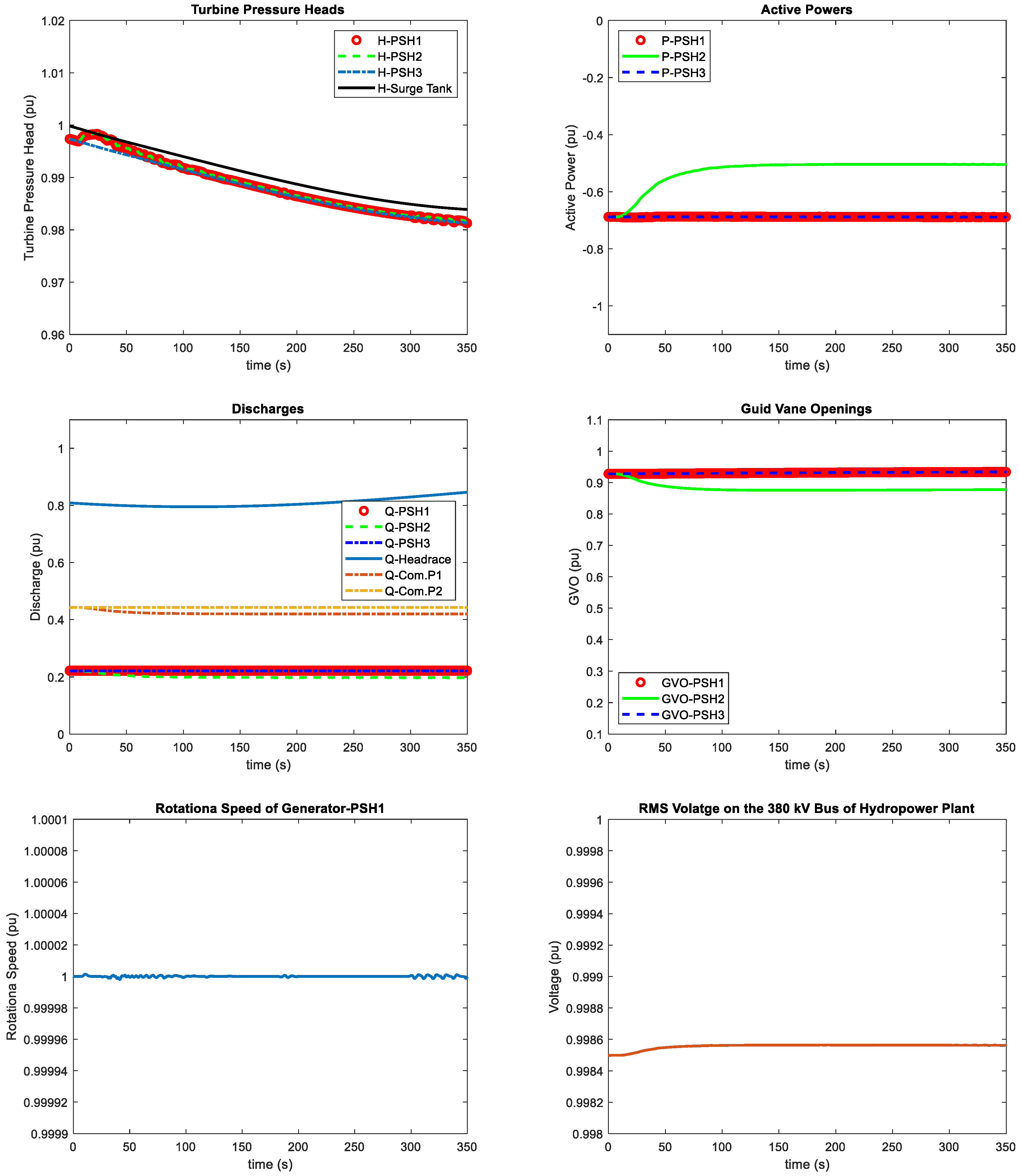
Figure 18. In the depicted results, the power set-point changes have a limitation ±0.01 pu/s for the maximum rate of change. It is important to mention that in the discharge diagram in
Figure 13,
Figure 14,
Figure 15,
Figure 16,
Figure 17 and
Figure 18, the base value for the discharge (water flow) is the rated discharge of the whole pumped-storage power plant which is four times more than the rated discharge for 1 PSH unit. Moreover, the water level in the upper reservoir stays constant with the rated amount of 1 pu in all the test conditions.
Table 2 summarizes different scenarios and important features for them.
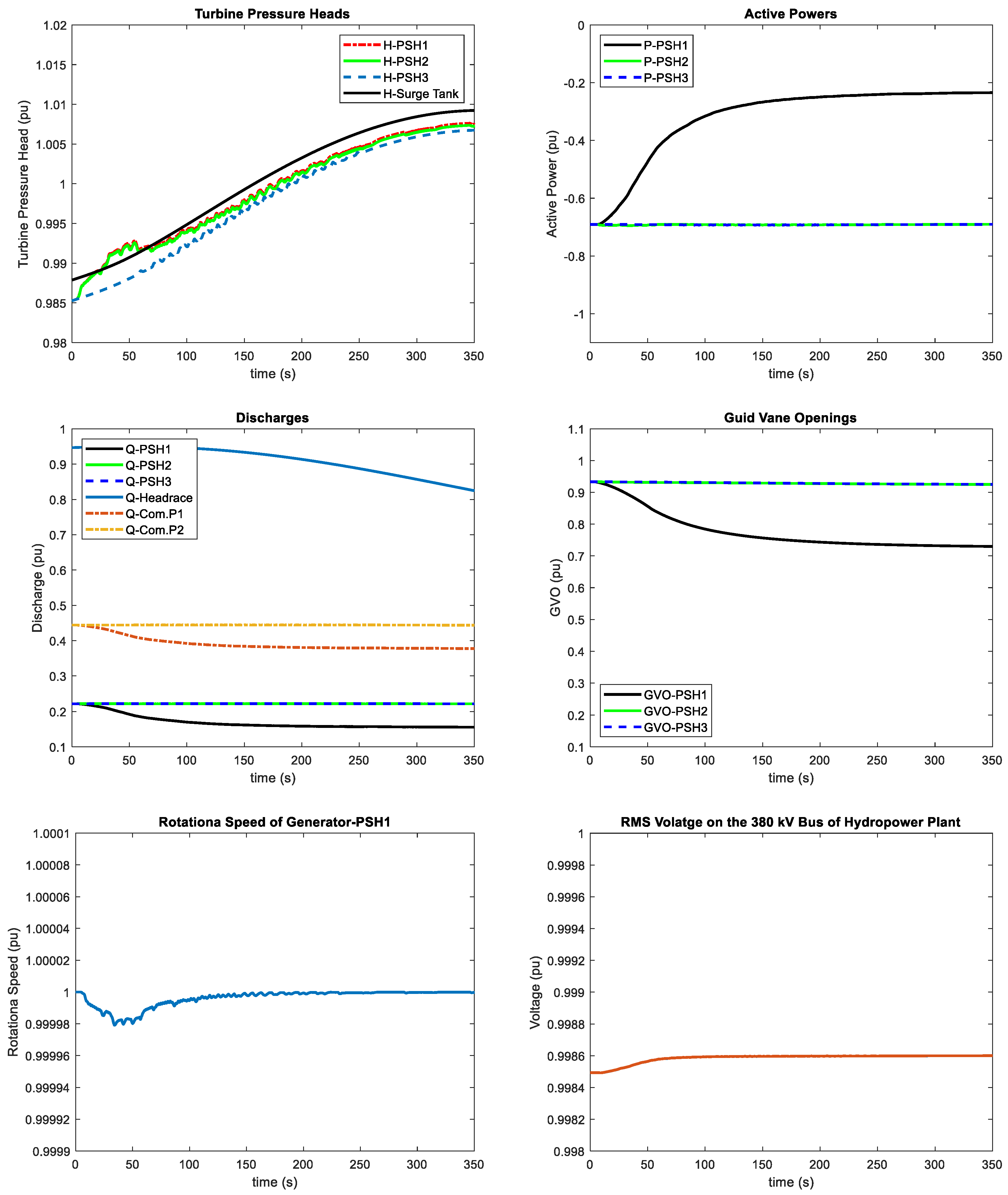
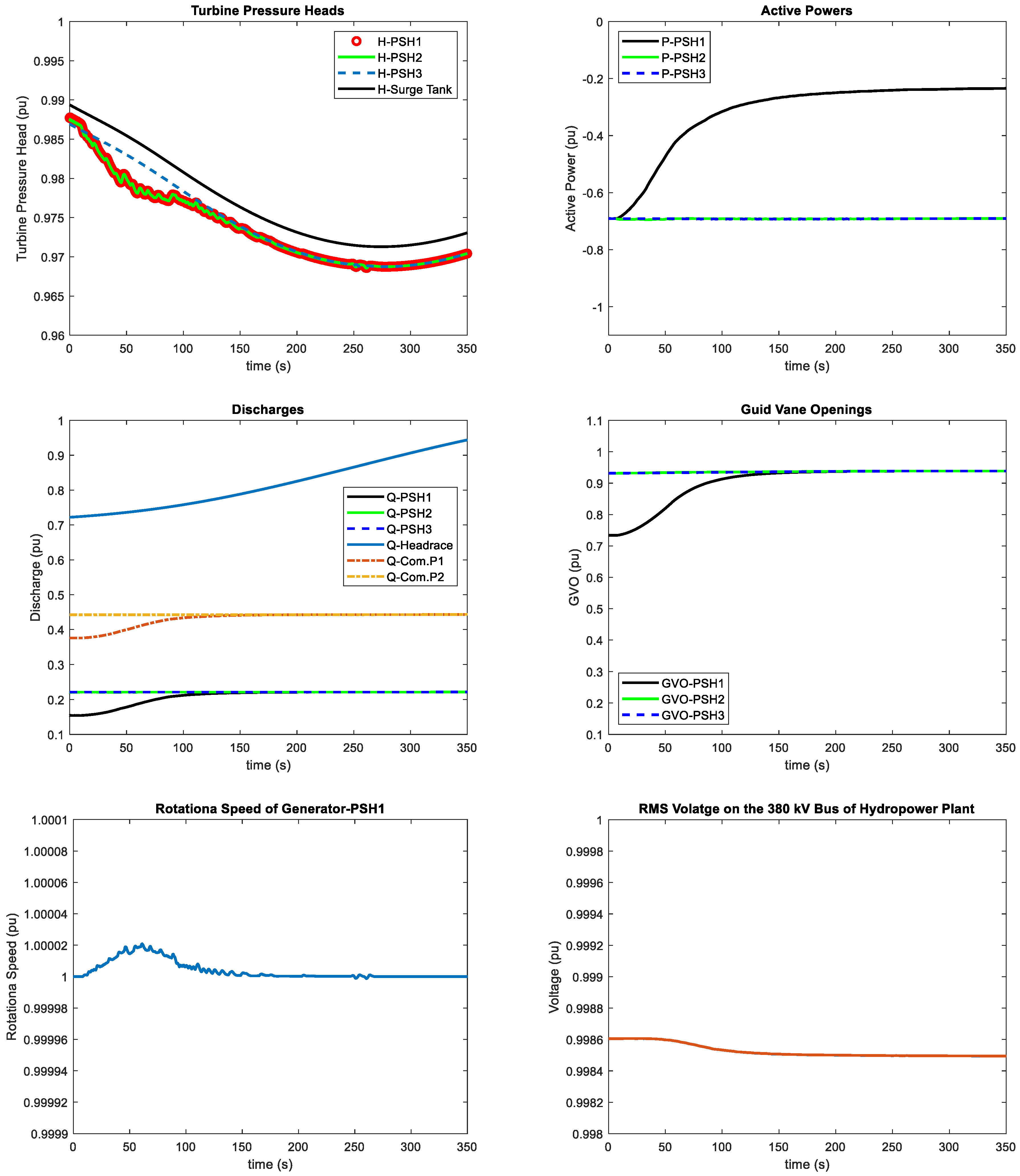
Figure 13 presents the RTDS results for decreasing the power set-point of PSH1 by 0.5 pu and the maximum rate of change as ±0.01 pu/s, while the power set-points of the other three units stay unchanged. By decreasing the power set-point of PSH1, its governor reacts and starts closing the guide vanes and this leads to a decrease in the discharge of PSH1 and consequently in the common penstock 1 discharge. In addition, changing the guide vane openings causes transient behavior in the pressure head. Since PSH1 and PSH2 are connected to the common penstock 1 with short separated penstocks, variations in the head and discharge in one unit can affect another one, e.g., there is head fluctuation in PSH2 due to the common penstock 1.
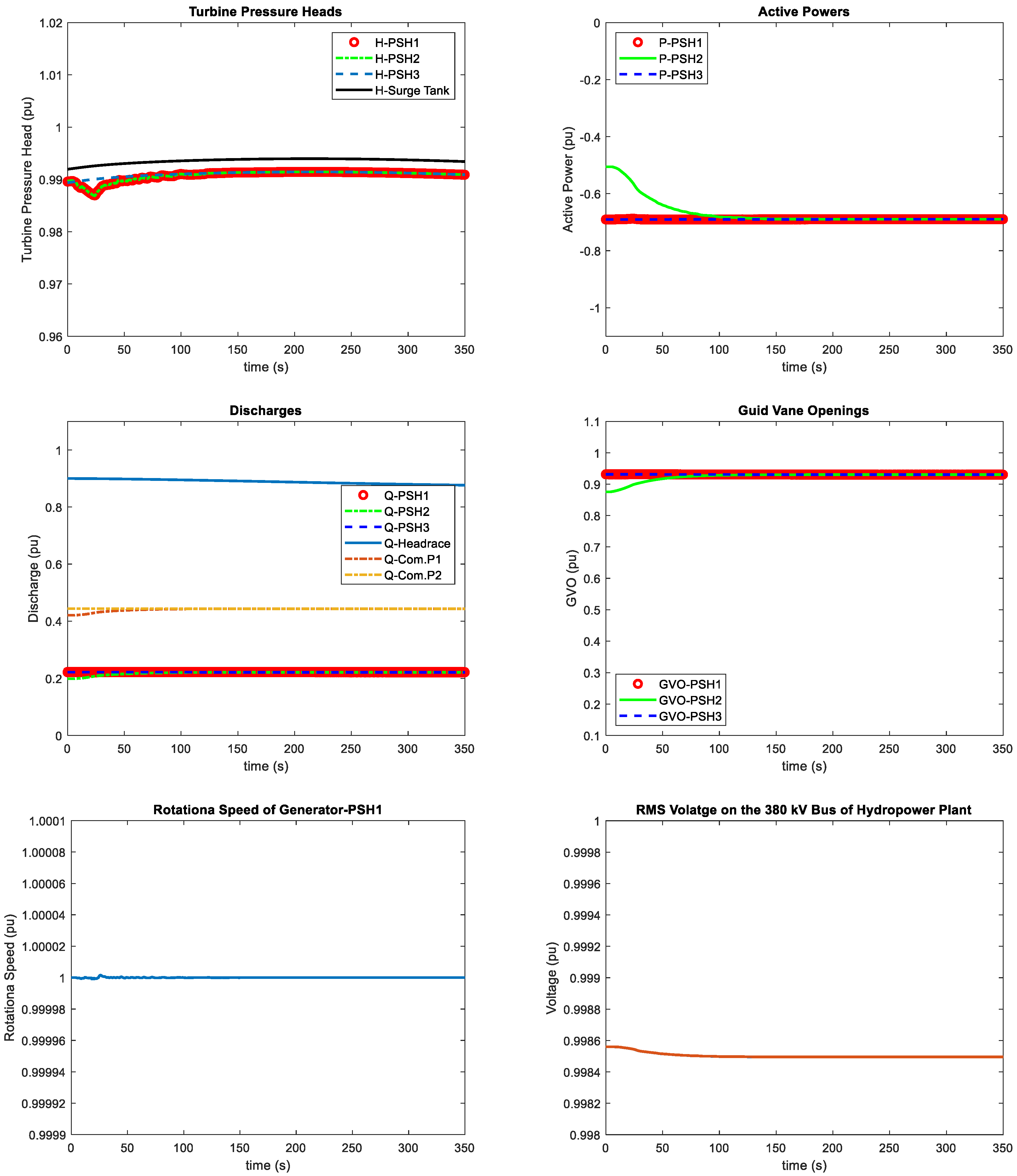
In
Figure 14, the RTDS result for increasing the power set-point of PSH1 by 0.5 pu and the maximum rate of change as ±0.01 pu/s is depicted, while the power set-points of the other three units stay unchanged. By increasing the power set-point of PSH1, its governor reacts and start opening the guide vanes and this leads to an increase in the discharge of PSH1 and consequently in the common penstock 1 discharge. Furthermore, opening the guide vanes causes transient behavior in the pressure head. Due to the presence of the common penstock 1 connected to PSH1 and PSH2 with short separated penstocks, changes in the head and discharge of PSH1 affect the head of PSH2.
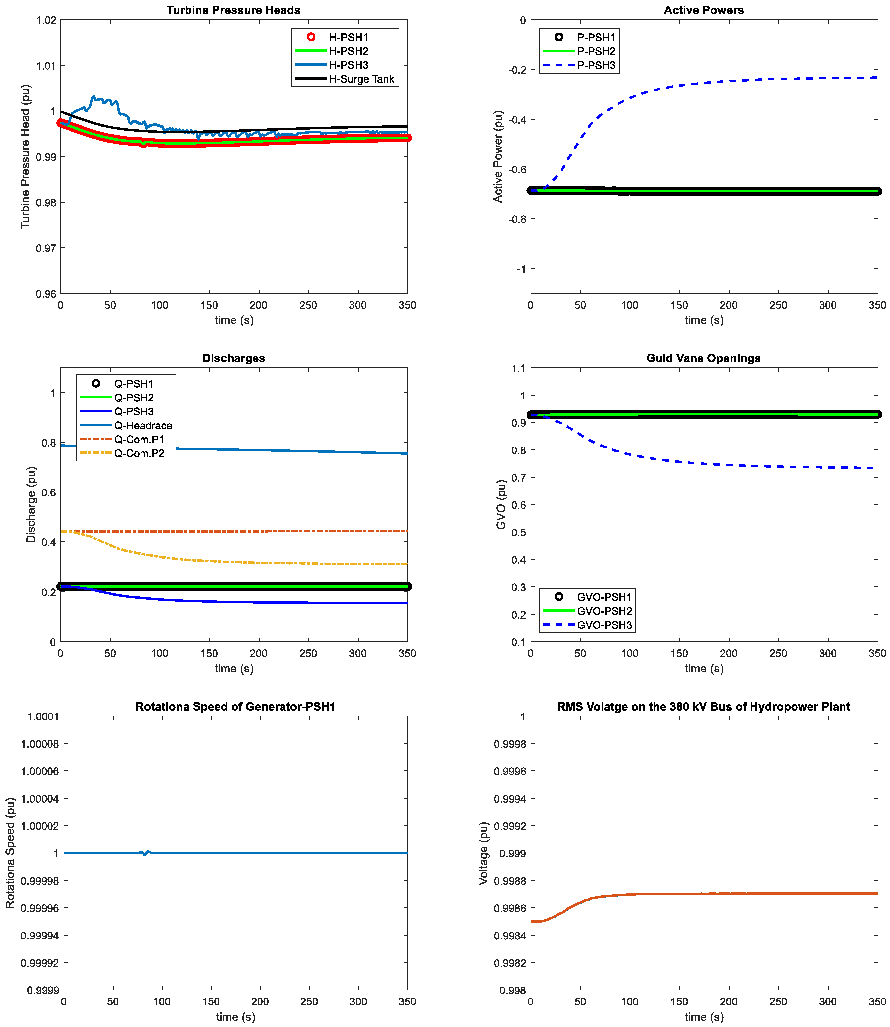
The RTDS results for decreasing the power set-points of PSH3 and PSH4 by 0.5 pu and the maximum rate of change as ±0.01 pu/s are presented in
Figure 15. As mentioned, both PSH3 and PSH4 are identical and only results for PSH3 are shown in
Figure 13,
Figure 14,
Figure 15,
Figure 16,
Figure 17 and
Figure 18. The governor systems of PSH3 and PSH4 try to reduce the guide vane opening positions of both units to control the active powers based on the power set-points. By comparing the turbine pressure heads in
Figure 13 and
Figure 15, the fluctuation in
Figure 15 is higher for PSH3 (PSH4) since two units are changing simultaneously. Moreover, in
Figure 15, the reduction in the discharge in the common penstock 2 is more significant than the test in
Figure 13, because, in
Figure 15, two units are reducing the output power, while in
Figure 13, only PSH1 is reducing the output active power.
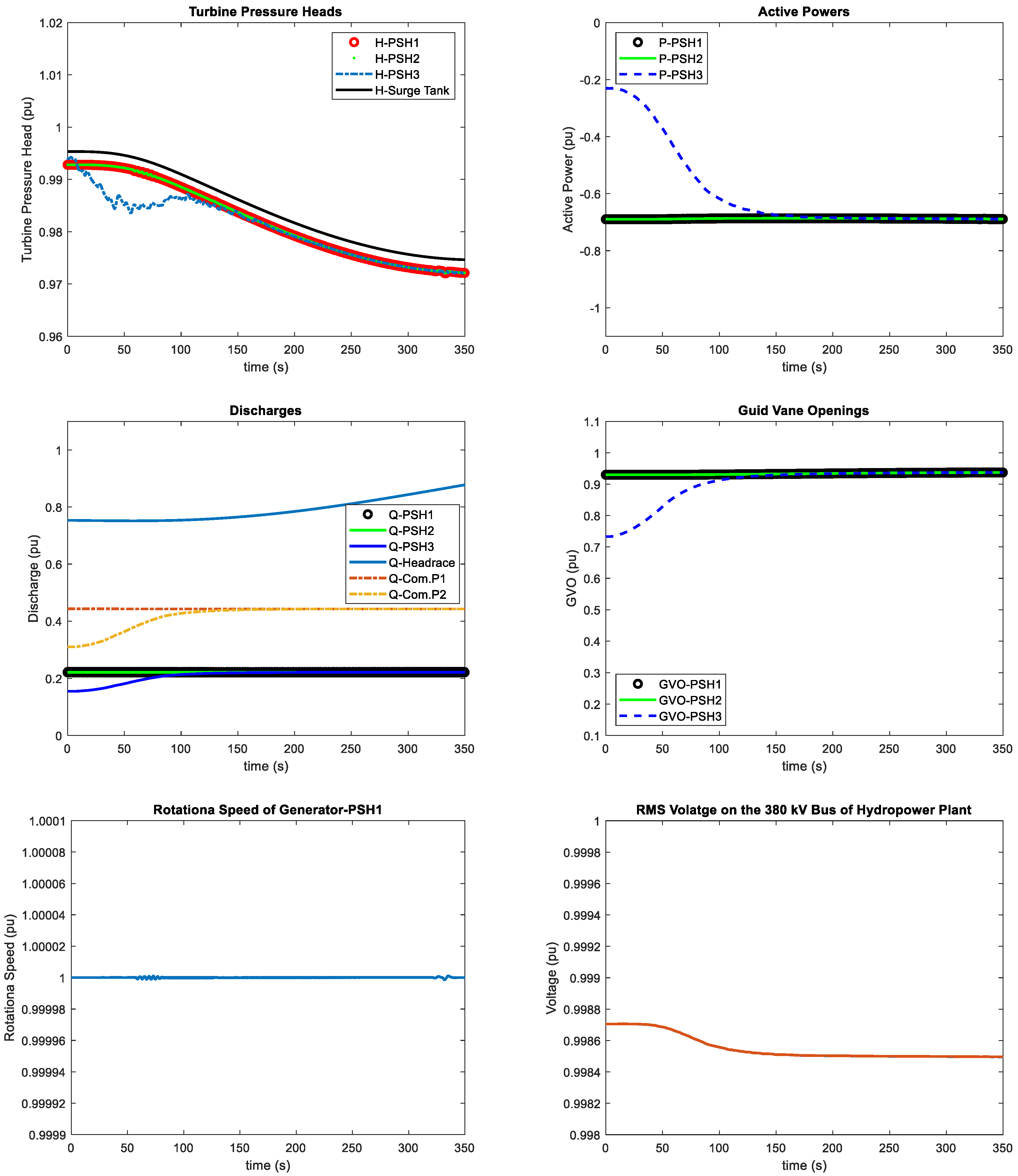
Figure 16 depicts the RTDS result for the reverse test in
Figure 15, which means that the power set-points of PSH3 and PSH4 are increased by 0.5 pu, while the power set-points of the other three units stay unchanged. The governor systems of PSH3 and PSH4 open the guide vanes to reach the new active powers based on the power set-points.
Figure 17 presents the RTDS result for decreasing the power set-point of PSH2 by 0.2 pu, while the power set-points of other three units stay unchanged. By decreasing the power set-point of PSH2, its governor reacts and start closing the guide vanes and this leads to a decrease in the discharge of PSH2 and consequently in the common penstock 1 discharge. Analogously to the other tests, changing the guide vane openings leads to transient behavior in the pressure head. Due to the common penstock 1, variations in the head and discharge of PSH2 causes head fluctuation in PSH1.
The RTDS results for increasing the power set-points of PSH2 by 0.2 pu with the maximum rate of change of ±0.01 pu/s are presented in
Figure 18. The changes in the power set-point leads to changes in the guide vane openings and this leads to changes in the water discharge and head of the PSH2. However, the changes in the discharge and head of PSH2 introduce changes in the head of PSH1 since they are connected to the common penstock 1 by short, separated penstocks. By comparing
Figure 13 and
Figure 14 to
Figure 17 and
Figure 18, it can be observed that larger changes in the power set-point can cause larger fluctuations in the head.
4. Discussion
In this publication, a power system consisting of a complex pumped-storage hydropower plant with four pumped-storage units, including 4 Francis pump-turbines, 4 short separated penstocks, 2 common penstocks, a surge tank, and a 14-km headrace tunnel are emulated and simulated in a real-time digital simulator (dSpace SCALEXIO) in the power hardware in the loop laboratory of the Institute of Power Systems at Graz University of Technology, and different conditions and events are tested to evaluate the capability of the RTDS.
The results demonstrate that changing the power set-point of the PSH1 has a significant effect on the head and discharge of the PSH2 and vice versa, since they are connected to the common penstock 1 with short, separated penstocks. This observation is also valid for PSH3 and PSH4 for the same reason, as they are connected to the common penstock 2 with short separated penstocks. In each unit, by changing the power set-point, the governor system adjusts the wicket gate positions that caused fluctuations in the head and discharge. Larger changes in the power set-point lead to larger fluctuations in the head of the turbine. The RTDS was able to demonstrate the hydroelectric interactions, as well as the transient and steady state behaviors of the hydraulic and electrical parts of all four units for various scenarios. This means that the computational performance of the RTDS can successfully emulate complex hydropower plants and it is a reliable testbed to use for future research studies in this field.
According to the laboratory results from the RTDS, we can draw the following conclusions:
An RTDS is capable of emulating the dynamic behavior of a complex pumped-storage hydropower plant with four units.
An RTDS is capable of presenting the dynamic hydro-electric behaviors of four PSHs with a common penstock and surge tank.
Last but not least, an RTDS can accurately emulate the hydraulic, mechanical, and electrical transients of a pumped-storage hydropower plant with a complex configuration.


