
Construction of Mixed Derivatives Strategy for Wind Power Producers

1
Faculty of Business Sciences, University of Tsukuba, Tokyo 112-0012, Japan
2
Faculty of Transdisciplinary Sciences for Innovation, Kanazawa University, Ishikawa 920-1192, Japan
*
Authors to whom correspondence should be addressed.
Energies 2023, 16(9), 3809; https://doi.org/10.3390/en16093809
Submission received: 29 March 2023
/
Revised: 18 April 2023
/
Accepted: 25 April 2023
/
Published: 28 April 2023
(This article belongs to the Special Issue Forecasting and Risk Management Techniques for Electricity Markets II)
Abstract
:Due to the inherent uncertainty of wind conditions as well as the price unpredictability in the competitive electricity market, wind power producers are exposed to the risk of concurrent fluctuations in both price and volume. Therefore, it is imperative to develop strategies to effectively stabilize their revenues, or cash flows, when trading wind power output in the electricity market. In light of this context, we present a novel endeavor to construct multivariate derivatives for mitigating the risk of fluctuating cash flows that are associated with trading wind power generation in electricity markets. Our approach involves leveraging nonparametric techniques to identify optimal payoff structures or compute the positions of derivatives with fine granularity, utilizing multiple underlying indexes including spot electricity price, area-wide wind power production index, and local wind conditions. These derivatives, referred to as mixed derivatives, offer advantages in terms of hedge effectiveness and contracting efficiency. Notably, we develop a methodology to enhance the hedge effects by modeling multivariate functions of wind speed and wind direction, incorporating periodicity constraints on wind direction via tensor product spline functions. By conducting an empirical analysis using data from Japan, we elucidate the extent to which the hedge effectiveness is improved by constructing mixed derivatives from various perspectives. Furthermore, we compare the hedge performance between high-granular (hourly) and low-granular (daily) formulations, revealing the advantages of utilizing a high-granular hedging approach.
1. Introduction
Wind power is considered to be sustainable and useful for green energy generation, and the installed capacity of wind power has rapidly increased in many countries and regions. Such an escalation in the installed capacity of wind power and the variability in wind power generation may give rise to considerable uncertainty for power industries operating in competitive electricity markets, as wind power output is volatile and largely contingent upon weather conditions. Owing to the uncertainty of the future and current wind conditions, wind power producers may suffer from the risk of volume fluctuations as well as price movement according to supply and demand in a short period (e.g., every half an hour). Consequently, price and volume simultaneously fluctuate, resulting in extreme volatility for the revenue or income cash flow of a wind power producer. To expand and support wind power generation businesses, even in a competitive environment, it is key to know how to control revenue and stabilize cash flow fluctuations effectively.
In this study, we construct a quantitative strategy for reducing the cash flow fluctuations of wind power producers in the electricity trading market using adequate financial instruments that are related to electricity prices, wind power generation, and weather indexes. Such financial instruments are called electricity derivatives [1] when the underlying asset is the price of electricity or the amount of electricity generated, and they are referred to as weather derivatives [2] when the underlying asset is an index composed of observed weather values, etc. Various instruments have been developed and proposed, as well as a number of optimal hedging techniques using derivatives in energy markets [3]. The use of derivatives and hedging transactions are widely practiced in today’s electricity market and have become an integral part of risk management for electric utilities [4,5]. In particular, weather derivatives are extremely useful for hedging energy market-related risks, and in recent years, there have been a large number of applications in both practical and research contexts [6]. Moreover, pricing methods and specific applications of weather derivatives are presented in several pieces of literature [7,8,9,10], where previous studies have been mainly related to weather derivatives on a single underlying index such as temperature [11,12,13,14,15,16], but also solar radiation/irradiation [17,18] and rainfall [19]. In the context of wind power businesses, the recent increase in hedging needs, coupled with the increased demand for wind power to achieve decarbonization goals, has led to recent studies on wind derivatives. There is a wide variety of derivatives, including the European put-type quanto options [20], barrier options [21,22], collar options [23], and wind call options [24], as well as the wind power futures (WPFs) [25,26,27], which are traded. Additionally, in a more recent study [28], the authors note that WPFs with area-wide generation as the underlying asset are not suitable for the effective hedging of individual generators, and factor futures with some principal components of individual generation as the underlying asset were proposed.
However, most of these studies have focused on the “pricing” of existing/standardized derivatives with single underlying indexes (Note that of the above studies, refs. [23,25,28] deal with hedging effects; however, it is still true that pricing challenges exist there). This fact is not surprising as the need for pricing, or the practical challenge, is inherent in those financial instruments themselves, i.e., standard-type derivatives. In other words, in the trading of standard-type derivatives, because the form of the derivative’s payoff function is determined in advance as a univariate function, the procedure whereby the buyer pays the seller an amount equivalent to the expected value of that payoff at the contract time (obtained from the “pricing”) is inevitable (assuming transactions between risk-neutral players and ignoring interest rates here). Moreover, the payoff functions of existing derivatives of the put or call types are not necessarily ideal ones for individual hedgers. For example, some studies [29,30,31] have proposed the use of a large number of put/call electricity derivatives along with the hedge volume risk in the electricity businesses. However, if the optimal derivatives can be designed and are tradable, they allow for more effective hedging while at the same time consolidating derivative contracts. Therefore, from the perspective of enhancing the hedge effect for individual hedgers, we adopt the so-called “flexible approach” that optimally synthesizes the payoff function (possibly a multivariate nonlinear function) to reflect individual hedge requests instead of existing standard-type derivatives.
The flexible approach has another advantage of solving the pricing issues of derivatives as illustrated in [32,33]. That is, it is demonstrated that any (European type) derivative can be designed by optimizing the payoff function with an expected value constraint of zero, which does not require payment procedures at the contract time. In other words, considering the “net payoff” of a derivative contract is the payoff at the maturity time minus the (fair) price at the contract time, and the essential issue of effective derivative design is to optimize this net payoff under fair trading conditions (i.e., expected net payoff equals zero). This derivative design was first applied in [32] for designing temperature derivatives in electric utilities and has been developed into various forms of derivatives transactions for prediction error losses [33], simultaneous hedging of price and volume [34,35], and mediated hedge trading model among different electric utility players [36]. A common feature of these studies is to use nonparametric regression techniques and to seek derivatives with arbitrarily nonlinear payoffs (nonparametric derivatives) for optimal hedging. Note that another approach to hedging that replicates arbitrarily nonlinear payoffs has recently been proposed in [37] based on the standardized derivatives, which were shown to be superior to nonparametric derivatives in terms of market transactions at the expense of hedging effect.
Thus, nonparametric derivatives have proven to be flexible and advantageous in terms of both hedge effect and contracting procedures efficiency. However, it is an open research question whether they can be applied to hedging the fluctuation risk of the product of price and volume in wind power businesses or whether (and how much) their effectiveness can be improved when using nonparametric derivatives with multiple underlying indexes. In other words, there exists a research gap in the absence of a modeling methodology or empirical analysis of this issue. Additionally, while recognizing the limitations of area-wide wind derivatives, as in [28], it may be possible to solve the problem of improving hedge effects by combining derivatives on weather variables as well as wind power generation; therefore, this study also addresses this interesting hypothesis.
In light of the aforementioned background, the present study proposes the utilization of nonparametric techniques to find optimal payoff structures or positions for mixed derivatives with fine granularity on the underlying indexes given by spot electricity price, area-wide wind power production index, and local wind speed and direction. Moreover, we develop a methodology for constructing mixed derivatives by modeling multivariate functions (related to payoff functions for multivariate derivatives) of wind speed and wind direction, where tensor product spline functions are applied to incorporate periodicity constraints on the wind direction. In the end, we demonstrate the enhancement of the hedge effect for mixed derivatives from various aspects based on empirical data. We also compare the hedge performance between high-granular (hourly) and low-granular (daily) formulations and reveal the advantages of utilizing a high-granular hedging formulation.
Note that this paper provides a new perspective on the simultaneous price and volume hedging problem by constructing derivative portfolios of multiple underlying assets and by elaborately modeling the nonlinear relationships among variables, which is distinct from our previous studies that have only dealt with volume risk [33,37]. Other related studies dealing with simultaneous price and volume hedging problems have been conducted for retailers [29,30,31,38], solar power producers [39], wind power producers [40], etc., but all of them deal with derivatives having a single underlying asset (e.g., electricity prices or temperatures). While some of our previous studies have also constructed multiple derivative portfolios for solar power producers and retailers [34,36], this study has a different objective in that it provides useful insights for wind power risk management practices and modeling challenges based on actual wind power generation data of wind farms (WFs) and other observation data for the electricity market and weather. In the context of a simultaneous hedging of price and volume, the quanto option, which has both of them as underlying assets, could be utilized (see, e.g., [41,42]). However, as previously noted, such conventional derivatives encounter challenges in terms of pricing and hedge effectiveness (thus, this approach was not employed). Furthermore, this study is not only new in constructing effective portfolios for the simultaneous price and volume hedging problem in the wind power business but also makes an unprecedented effort to examine in detail the modeling techniques that enhance the hedge effect. For example, the viewpoint that hedge effects can be improved by combining (original) local wind speed derivatives in addition to (commonly traded) area-wide wind generation derivatives would provide a useful perspective for both power producers and financial product designers. In addition, we demonstrate other multifaceted empirical analyses that have not been focused on in previous studies, such as the use of lag variables in the design of underlying assets, testing the robustness by varying in-sample and out-of-sample periods in multiple scenarios, and understanding hedge effects using different indicators.
The remainder of this paper is organized as follows. In Section 2, we start with motivational arguments on the policy mechanisms related to renewable power trading and formulate the optimal hedging problem with mixed derivatives. We construct a concrete hedging model, detail the underlying assets considered and the method of modeling nonlinearity, and provide data description and performance measures. Section 3 presents the results of the empirical analysis from various perspectives. In particular, we clarify the hedge effects across multiple hedging models and the choice of underlying indexes with a detailed discussion of effective modeling approaches and their implications. In Section 4, we compare the hedge performance between high-granular (hourly) and low-granular (daily) formulations and reveal the advantages of utilizing a high-granular hedging formulation. Finally, we provide conclusions in Section 5.
2. Optimal Hedging with Mixed Derivatives
2.1. Motivation
We begin with motivational arguments on policy mechanisms related to renewable power trading. Among several policy mechanisms for enhancing renewable energy development, the feed-in tariff (FIT) is probably the most commonly introduced method in many countries [43]. Under the FIT mechanism, wind power producers are generally protected from price risk; that is, the sales price of the power output is guaranteed for a certain long-term period. In this case, it is sufficient for wind power producers to hedge volume risk using derivatives with suitable underlying indexes related to wind power variability. A potential candidate for such an underlying index is the wind power production (WPP) index, which denotes an area-wide production of wind power in a country, such as the German wind power index listed in Nasdaq [44], to hedge the production of wind power in Germany. Such a WPP may be effective for groups of WFs covering a wide area but may be challenging to use for individual WFs because of the strong local effect of weather. In addition, the WPP index must be standardized and managed under a solid rule to guarantee the fairness of data. Another candidate for a wind-related index is to use publicly available wind weather condition (WWC) data, such as wind speed and direction observed by a meteorological weather station in the local area. The advantage of such a WWC index is that weather data are objective and observed at many different places with the same quality and that WFs may incorporate local wind conditions near their locations.
There is an updated policy mechanism called the feed-in premium (FIP; see, e.g., [45]), under which wind power producers sell the power output at a market price and receive an additional payment (premium). Both FIT and FIP mechanisms provide an incentive for business owners to develop wind power generation projects in the corresponding country, but an essential difference is that, under FIP, wind power producers need to be concerned with the risk of price as well as volume fluctuations. The introduction of FIP is aimed to integrate the renewable energy development business into a market-oriented environment where the sales price changes according to the competitive market price. This situation is the focus of this study, under which wind power producers may suffer from the risk of simultaneous fluctuations in price and volume, and it is the key to know how to stabilize their revenues (or cash flows) for trading wind power output effectively in the electricity market.
To manage the risk of cash flow fluctuations determined by the price and volume, wind power producers may use electricity derivatives whose underlying index is given by the spot electricity price, in addition to wind derivatives on WPP and WWC indexes. However, it would be more desirable for wind power producers to use mixed derivatives of electricity prices and wind-related indexes using a multivariate payoff function if there exists a suitable methodology. Our study is based on this point of view, i.e., we would like to develop a methodology to optimally construct mixed derivatives on wind indexes and electricity prices for wind power producers (i.e., WFs) and control their cash flows against the simultaneous fluctuation of electricity price and wind power generation.
2.2. Minimum Variance Hedging Problem
The goal of hedging is to replicate the target cash flow using another cash flow that is defined by the payoff of a portfolio of derivative contracts with effective underlying indexes. In this context, we provided a methodology to construct a derivative portfolio of weather and energy derivatives using nonparametric regression techniques for power retailers and photovoltaic (PV) generators [34]. This idea has been extended to the case where power retailers and generators (PV or thermal generators) trade through the central exchange market, and an insurance company handles weather and electricity derivatives or forward contracts between them [36]. In this study, we extend our previous work to the hedging problem of wind power producers and formulate mixed derivatives by specifying various types of payoff functions.
Let [kWh] be the power output of a WF that can be sold at the spot electricity price, denoted by , in the corresponding area for delivering electricity in the (hourly) time interval , where we assume that the basic period is an hour and all variables are observed at least hourly. Note that changes with wind conditions, whereas is volatile depending on the supply and demand at the moment; hence, the revenue (or the cash flow) from electricity sales, defined by , may be extremely volatile.
To reduce the risk of cash flow fluctuations, we introduce the following minimum variance hedging problem using mixed derivatives on spot electricity price and WPP and WCC indexes and :
where represents the variance and denotes a payoff function of mixed derivatives, which is optimized subject to the zero-mean condition . In (1), may contain the wind speed and direction observed by a meteorological weather station near the WF; is the total wind power generation in a country or region, covering all locations of the WFs. We use the total wind power generation data in the (hourly) time interval denoted by in the electricity network observed by the independent system operator (ISO). Note that is an area-wide index and that only one representative variable is observed. On the other hand, the dimensions of and depend on the number of meteorological weather stations near the wind farm. If there are multiple observation points, each variable of or becomes multidimensional to incorporate multiple wind speeds or directions observed at different stations.
In our approach, we formulate European-type derivatives by optimizing payoff functions, subject to the expected value constraint of zero, without involving any upfront payment obligations at the contract initiation, thereby leading to derivative contracts with an initial value of zero. In this context, the crux of effective derivative design lies in the optimization of the “net payoff” under fair trading conditions wherein the expected net payoff is set at zero; the “net payoff” of a derivative contract is defined as the payoff at maturity minus the (fair) price at the time of contract initiation (which is set as zero in our approach).
Furthermore, it is noteworthy that wind power generation can be technically formulated by a cubic equation for wind speed, which accounts for Betz’s law [46,47]. However, in practical application, there is also a certain correlation between the wind direction and the wind power generation, as wind speed is measured at a specific point. As a result, wind direction is often incorporated as an explanatory variable in contemporary wind power forecasting models [48]. Thus, the incorporation of local wind speed and wind direction information in addition to area-wide power generation data is anticipated to provide a more precise depiction of individual wind power generation patterns and potentially enhance the effectiveness of hedge effects with mixed derivatives.
2.3. Construction of Hedging Models
In this study, we apply three types of regression models, corresponding to linear hedging, spline hedging, and tensor hedging, respectively, for solving (1), and evaluate their hedge effects.
2.3.1. Linear Hedging
At first, we demonstrate the following linear regression of on covariates as a benchmark, namely “linear hedging”, which provides the simplest hedging strategy for solving (1):
where is a coefficient vector to be estimated and is the residual term in the linear regression. In Equation (2), the regression coefficients provide optimal investment units of forward contracts on the underlying indexes for controlling the cash flow deviation from by assuming that the physical probability measure provides a risk-neutral probability measure. This is because forward prices are given by their mean values under the risk-neutral probability measure, and the following condition holds with the optimal regression coefficient vector and residual :
(In this paper, the overline notation, e.g., , is used to denote the mean value. Note that the notation below is used to denote that is defined to be ).
Then, we see that minimizing provides the optimal value of the objective function by letting:
In other words, the residual corresponds to the optimally hedged cash flow using forward contracts on ; therefore, we may conclude that solving the minimum variance hedging problem (1) with forward contracts can be achieved through linear regression of (2).
2.3.2. Spline Hedging
Next, we introduce a nonparametric regression,
characterized by smoothing spline functions and being multiplied by (called a by variable; see [49]), where is the intercept and is the residual. The regression problem (3) may be solved as a generalized additive model (GAM [50,51]) using univariate smoothing spline functions and to minimize the residual sum of squares with a penalty on smoothness. In this study, we refer to the hedging strategy obtained from (3) as “spline hedging.”
A common structure of each regression function in (3) is to have as a by variable of smooth terms [49] that is introduced precisely against the price risk, and its interaction with wind power generation is incorporated. That is, the sum of spline functions, is multiplied by to hedge the simultaneous fluctuation of price and wind power generation.
The regression Equation (3) provides minimum variance hedging using derivatives on Even though derivative prices are not explicitly incorporated, it can be shown that the resulting residuals from the regressions provide hedged cash flows in the objective function of (1) under the same assumptions as those for (2). Then, the optimal payoff function may be obtained using the regression functions in (3) as
2.3.3. Tensor Hedging
Third, we further incorporate the wind direction in the first term of (3) and consider the following regression:
Compared with (3), we see that the first term in (4) is extended to incorporate the nonlinearities of wind speed regarding power generation and the cyclic feature of wind direction . Note that the bivariate smooth function is represented as a tensor product spline function of , which is a multidimensional smooth function that is expressed by a tensor product. Because separate basis functions may be specified in tensor product spline functions, we set a cyclic smoothing basis for the -direction and a cubic spline basis for the -direction to solve the regression problem in (4), where the cyclic smoothing basis enables us to model a periodic function whose endpoint smoothly connects with the initial point (see [51] for the definitions of tensor product and cyclic spline functions). Then, the regression problem (4) may be solved as GAM and the optimal payoff function may be obtained using the regression functions in (4) as
2.3.4. Incorporation of Lagged and forward Variables
Moreover, we assume that each variable related to the WPP and WCC indexes may be multidimensional when observation data for multiple meteorological weather stations and/or lagged variables of and are used. In such a case, additional spline functions or linear terms are added to (2)–(4). For example, when and are both two-dimensional with and , (2)–(4) are modified as
where and are univariate smoothing spline and bivariate tensor spline functions, respectively, and is a coefficient vector with appropriate dimensions.
Another noteworthy issue is the enhancement of covariates by incorporating lagged and forward variables. The effect of wind conditions may not be direct, and lagged or forward variables may contribute to the improvement in hedge performance because the meteorological weather stations chosen in our experiment are not neighbors (approximately 10 km or more from the wind farm). A similar consideration may be applied to the relationship with the WPP index. In this study, we examine the effect of lagged and forward variables in covariates, on the hedge performance (see Section 3.2).
2.4. Performance Evaluation Measures
We estimate the optimal regression functions and other required parameters in (2)–(4) using the data in the learning period and subsequently evaluate the hedge performance using the out-of-sample data in the test period. More specifically, we execute out-of-sample hedge simulations by substituting the observed data in the test period into the estimated regression Equations of (2)–(4) to compute the predicted values of the target variable . In this case, the deviation of from the expected cash flow is hedged using the payoff of derivatives , where may be considered as an unhedged cash flow for the wind power producer. Note that the payoff functions are extracted from the estimated regression Equations in (2)–(4), and the difference between the predicted and realized values for provides out-of-sample hedge errors. Like our previous study in [32,36], we use the following variance reduction rates (VRRs) and normalized mean absolute errors (NMAEs) to evaluate the hedge performance in the out-of-sample case:
where denotes the out-of-sample hedge errors in the test period.
To test the robustness of the proposed model, we also consider the following hypothetical in-sample case. That is, instead of using the estimation result of the learning period to compute out-of-sample hedge errors, we can estimate the regression functions and compute hedge errors using the same data as the test period. In this case, the test period becomes in-sample, and we refer to the resulting hedge errors as in-sample hedge errors. The in-sample hedge errors provide a measure of the “best hedge” based on the same model and data, and the comparison of out-of-sample hedge errors with in-sample hedge errors allows us to understand the performance degradation from the best hedge. For in-sample hedge errors , we define VRR and NMAE in the in-sample case as
2.5. Data Description
We used the power generation data [kWh] from two individual WFs located in the Kyushu and Chubu areas, Japan, which have the data periods of 1 October 2019 to 30 September 2022 for the WF in Kyushu and 1 October 2019 to 31 March 2022 for the WF in Chubu. The data were observed every 30 min, but we used hourly data to adjust the data frequency to those of the WPP and WCC index data. For the WPP index, we used area-wide wind power generation data, [MWh], released by the general power transmission and distribution business operator, whose function corresponds to the ISO in Japan and is obligated to guarantee final power transmission and distribution in addition to balancing the entire electricity network in the area. For the WCC index, we used wind speed [m/s] and cardinal direction categorized into 16 directions. We assigned to the cardinal direction starting from the north clockwise direction. Finally, we used the JEPX spot price, which is the price of spot electricity to deliver electricity during a predetermined half-hour slot and which is executed under the single price auction system in the day-ahead market (see http://www.jepx.org/english/outline/index.html, accessed on 10 April 2023). Here, we take the hourly average to obtain hourly data, denoted by [JPY/kWh].
For the wind farm located in the Kyushu area, we chose two weather observation stations whose distances from the wind farm were approximately 10 and 12 km, respectively. For the wind farm in the Chubu area, we chose four weather observation stations whose distances from the wind farm were approximately 13, 16, 18, and 25 km, respectively. The JEPX spot prices, WPP indexes for Kyushu and Chubu, and weather data were downloaded from the following websites, respectively:
- http://www.jepx.org/market/index.html (JEPX Kyushu area price and Chubu area price, accessed on 27 March 2023).
- https://www.kyuden.co.jp/td_service_wheeling_rule-document_disclosure (WPP index, Kyushu, accessed on 27 March 2023).
- https://powergrid.chuden.co.jp/denkiyoho/ (WPP index, Chubu, accessed on 27 March 2023).
- https://www.data.jma.go.jp/gmd/risk/obsdl/ (WWC Index, Japan Meteorological Agency, accessed on 27 March 2023. Note that missing values were imputed using linear interpolation.).
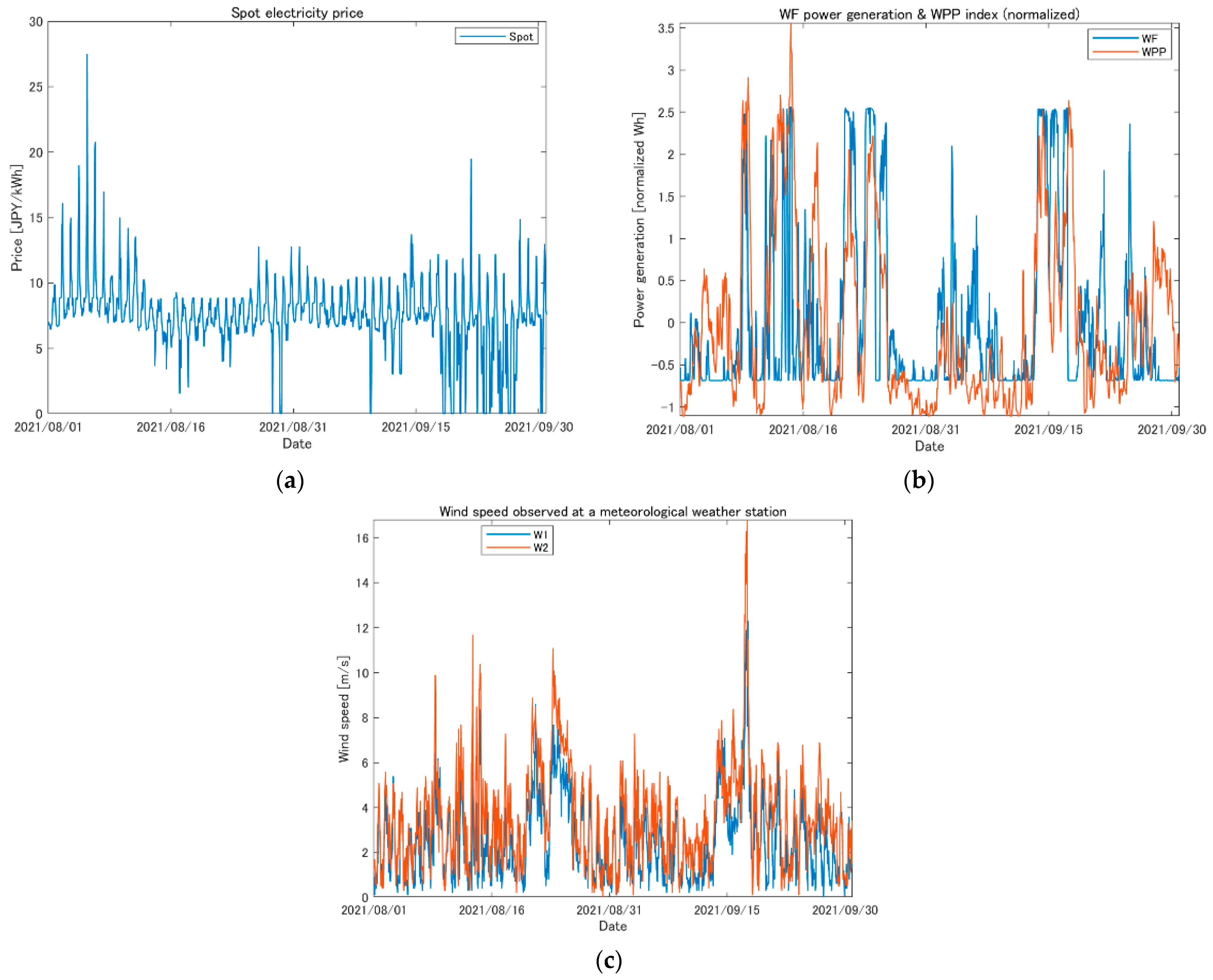
Panels (a)–(c) in Figure 1 respectively demonstrate the historical data of the Kyushu area spot electricity price, WF power generation with the WPP index, and wind speed data observed at two meteorological weather stations for two months in the data period (i.e., 1 August–30 September 2021). Note that the WF power generation and WPP index are normalized by the mean and standard deviation for comparison based on the same scale.
In this study, all regression models were estimated using R 4.2.2 software (https://www.R-project.org/, accessed on 19 March 2023) using the mgcv package [49] for applying GAM, wherein the smoothing parameter is calculated using the generalized cross-validation criterion. Some figures were plotted using MATLAB 2022a (MathWorks, Inc., Natick, MA, USA).
3. Empirical Performance of Hourly Hedges
We estimate the optimal regression functions and other required parameters in (2)–(4) using the data in the learning period and subsequently evaluate the hedge performance using the out-of-sample data in the test period. Here, the learning and test data periods were set as follows (see Appendix A for descriptive statistics of variables):
- Learning period: 1 October 2019 to 30 September 2020. (Hourly data, number of data observations: 8784)
- Test period: 1 October 2020 to 30 September 2021. (Hourly data, number of data observations: 8760)
In this section, the two-year data period was split in half as shown above, but a further investigation into the relation of the lengths between learning and test periods would be interesting and should be considered as a future research topic.
3.1. Estimated Smooth Functions
Here, we demonstrate estimated smooth functions when regression Equation (4) is applied for the learning period of the data to hedge the cash flow fluctuation of WF in Kyushu. Note that such smooth functions provide a payoff function of mixed derivatives as:
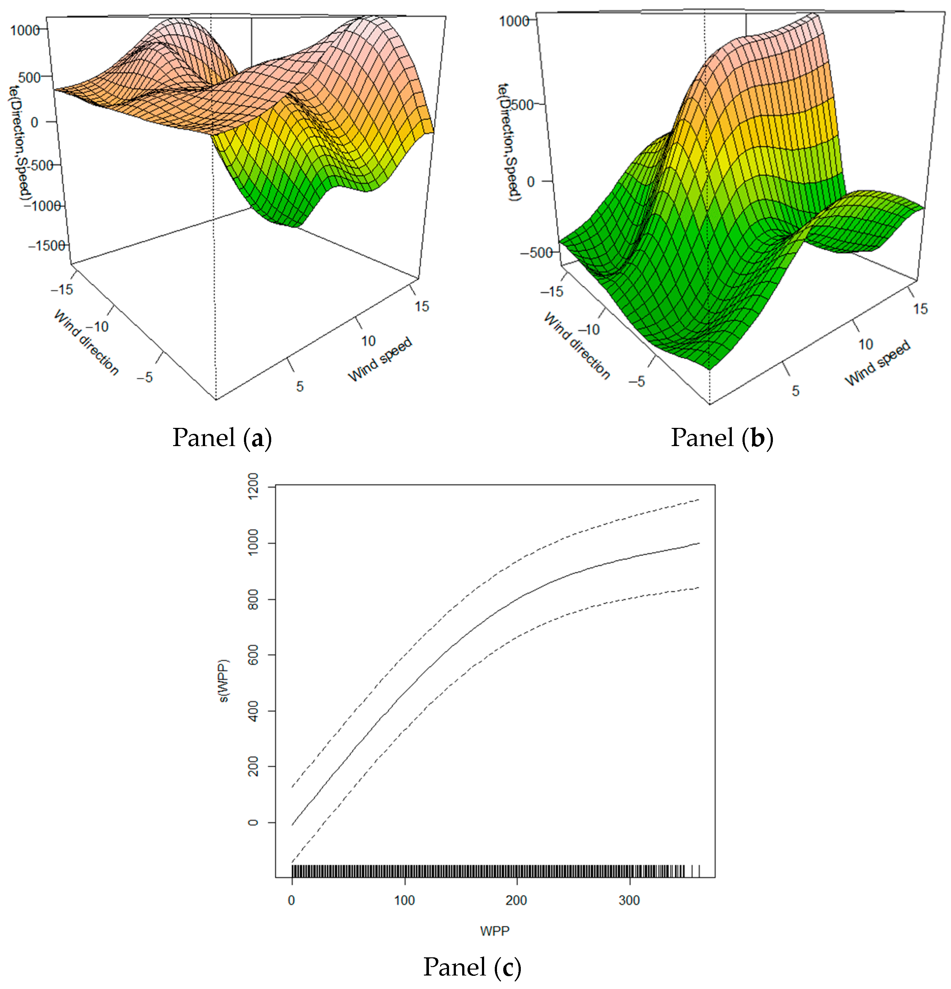
Panels (a) and (b) in Figure 2 illustrate the estimated univariate and tensor spline functions of and , respectively, where two tensor spline functions (Panels (a) and (b)) and one univariate spline function (Panel (c)) were estimated as there were two observation points of WCC indexes in the case of the WF in Kyushu. We observe that the estimated univariate spline function reflects the positive effect of the WPP index on cash flow and is nonlinear for large values of the WPP index. On the other hand, the estimated tensor spline function depicted in Panels (a) and (b) represents the interaction between wind speed and direction concerning the target cash flow and can model the cyclic property of the wind direction.
Based on the estimated tensor spline functions presented in Panels (a) and (b), it becomes evident that an intricate interplay exists between the variables of wind direction and wind speed. Furthermore, this interaction exhibits dynamic changes that are contingent upon the location of the observation point relative to the installation site of WF. It is noteworthy that the configuration of the payoff function is prone to undergo significant changes in the presence of high wind speeds, owing to the limited number of samples available for such cases (For example, outlier data may arise in the context of catastrophic typhoons, leading to the shutdown of wind turbines. There may be potential for exploring additional insurance mechanisms, such as compensation for generator emergency shutdowns that are infrequent in occurrence. However, it should be noted that such considerations are beyond the scope of this study).
It should be noted that one of the advantages of using nonparametric regression models such as GAM is not only the incorporation of the nonlinear effects of covariates but also the ease of interpretation by visualizing the estimated functions [52]. Such a visualization helps us understand the structure of payoff functions for derivatives, as multivariate derivatives may have complex payoffs that need to be specified before executing derivative contracts. Moreover, the ease of interpretation provides an important factor in building consensus and ensuring the reliability of the model as well as accuracy in electric utility practice [53]. In addition, the use of GAM allows us to obtain statistical interpretation as well, similar to other statistical models, although we have omitted the details for brevity.
3.2. Effect of Lagged and Forward Variables
Now, we demonstrate the out-of-sample results for our hedge simulations. As aforementioned, the out-of-sample hedge simulations were executed by substituting the observed data in the test period into the regression equations and computing the hedge errors given the estimated smooth functions and coefficients of (2)–(4) using the learning period of the data. Here we examine the hedge effect using VRR and NMAE mainly based on the bar graphs shown in Figure 3 and Figure 4. Note that the numerical results are listed in table formats in Appendix B.
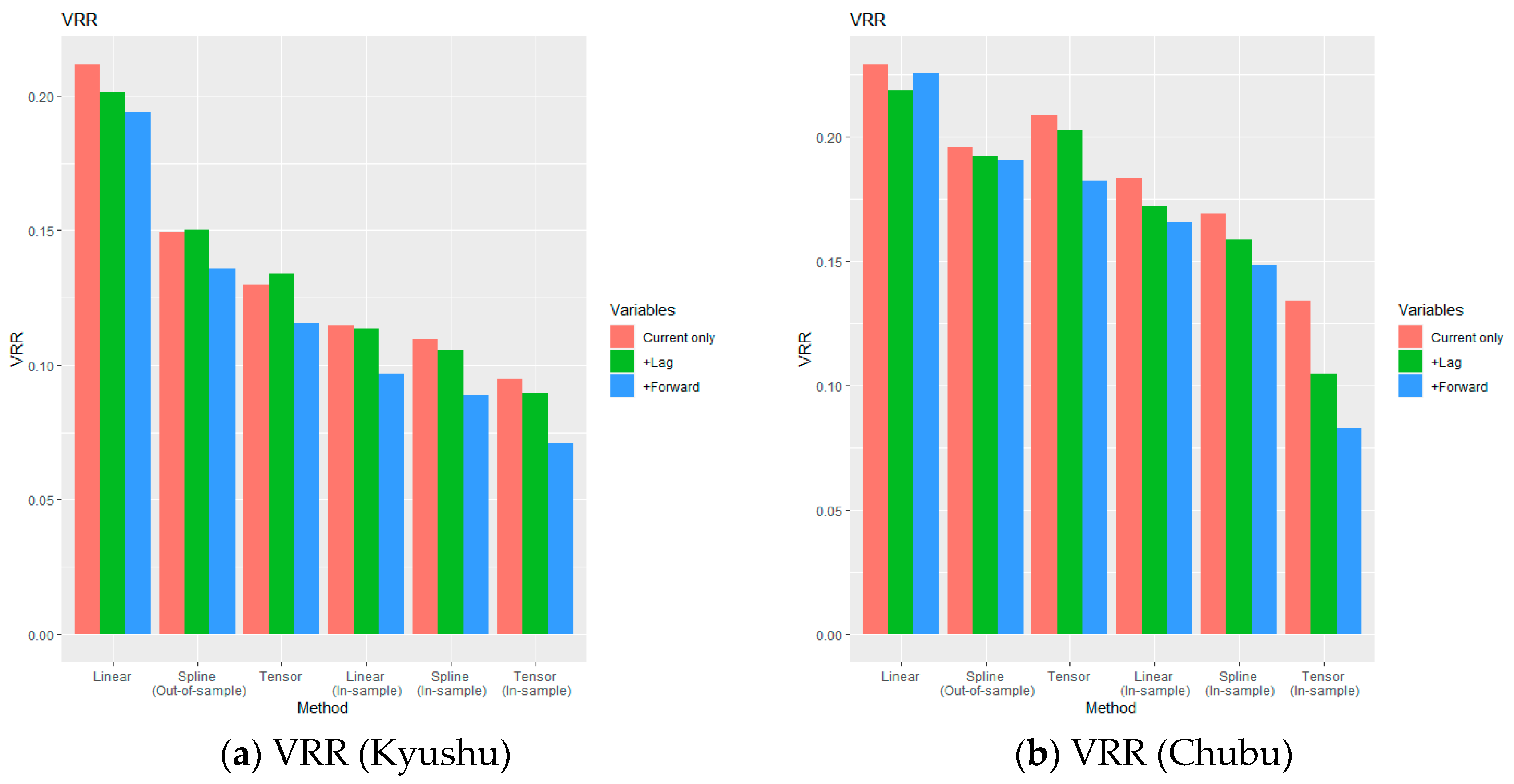
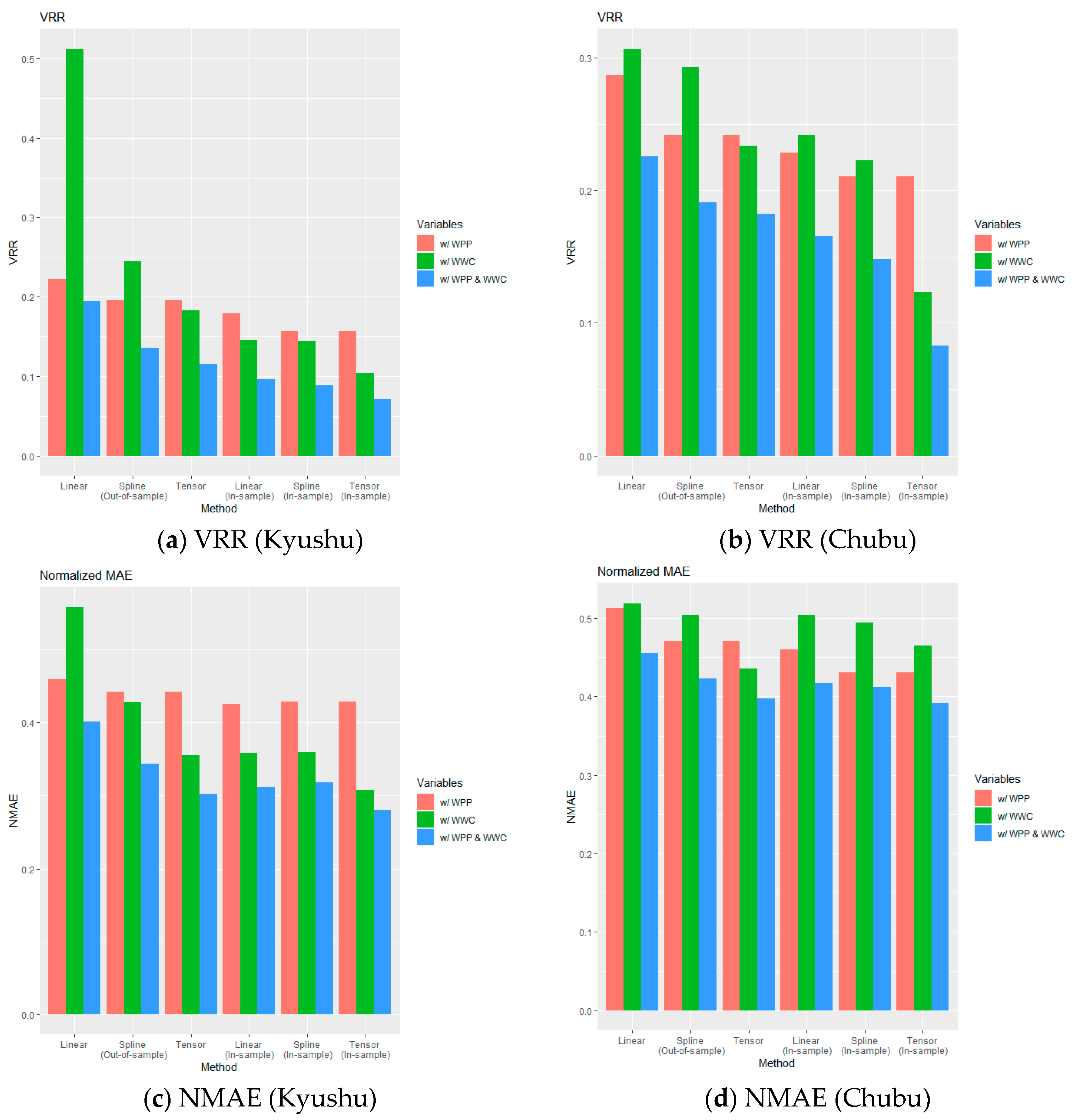
The left and right three sets of bins in Panels (a) and (b) in Figure 3 compare the VRR in the out-of-sample case with those of the in-sample case when different hedges (i.e., linear hedging, spline hedging, and tensor hedging) are applied for the cash flows of the wind farm in Kyushu and Chubu, respectively. The red bins represent the cases in which the target cash flow is regressed concerning covariates with the same observation period only. On the other hand, one period of lagged variables are added for the green bins and one period of forward variables are further added for the blue bins.
When we focus on the same choice of covariates, we see that the hedge performance measured by VRR improves by taking nonlinear effects into account in the regression equations, even for the out-of-sample case. Although the hedge model using tensor product splines (i.e., tensor hedging) can reflect the effect of wind direction and provide the best hedge performance in Figure 3 among all the cases, it sometimes becomes worse compared with spline hedging. However, tensor hedging achieves the smallest VRR among all out-of-sample simulations when lagged and forward variables are added, and the incorporation of lagged and forward variables almost always improves the out-of-sample VRR. In these simulations, the smallest VRR for the out-of-sample case was 11.5% for Kyushu and 18.2% for Chubu, indicating that the variance of the target cash flow was reduced by 88.5% or 81.8% using derivatives with tensor product spline functions.
Note that the in-sample VRR is also plotted as the three sets of bins on the right. In the case of in-sample simulations, we see the improvement of the VRR concerning the choice of methods and effect of adding variables more clearly. In addition, although the out-of-sample VRR for Chubu using tensor hedging achieves a reasonably good value of 18.2%, the performance was degraded compared with the best (in-sample) VRR of 8.30%. This indicates that there is some room for improvement for out-of-sample hedges, and further investigation to reduce the gap may be effective.
A similar tendency was observed when NMAE is plotted instead of VRR as shown in Panels (c) and (d) in Figure 3 where NMAE, which is defined in Section 2.4, provides a measure of improvement for the hedges in terms of mean absolute errors relative to unhedged cash flows. In the two simulations for Kyushu and Chubu, the in-sample NMAE and out-of-sample NMAE are not significantly different, indicating that the performance degradation is not very noticeable. Note that the residual sum of squares minimized in the regression problems is closely related to variance minimization; in this sense, VRR may be more suitable as a performance measure for hedges in our approach. However, an evaluation using mean absolute errors or mean squared errors is also worthwhile because they have often been used to evaluate the out-of-sample performance of recent machine learning approaches. In the case of out-of-sample simulations using tensor hedging, we see that the sizes of deviations for the cash flows were reduced by 70% and 61% for Kyushu and Chubu, respectively.
3.3. Effect of Individual Wind Power Related Covariates
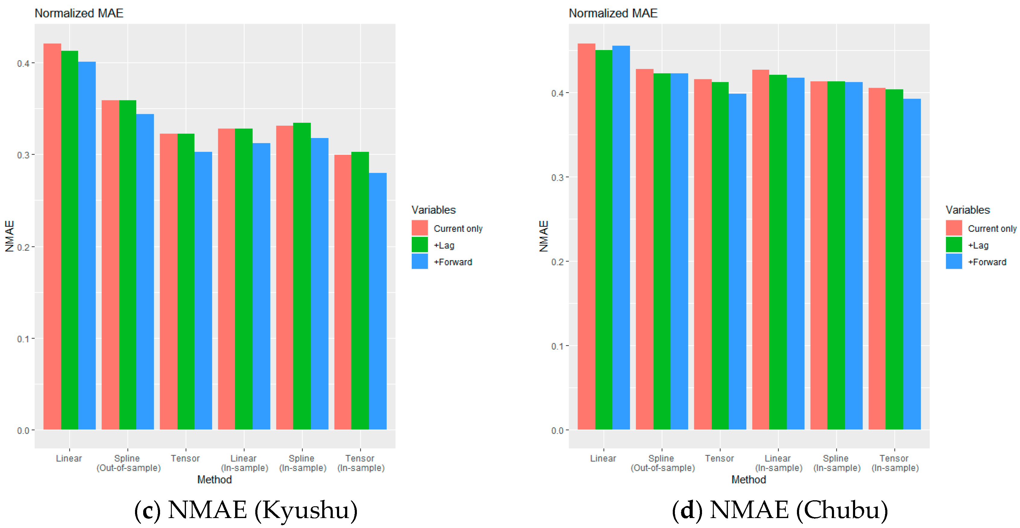
Next, we compare the hedge effects for different combinations of underlying indexes. Given that the focus of this study pertains to the hedging problem associated with the combined risks of price and volume, it is imperative to utilize electricity futures, with the spot electricity price serving as the underlying index, as a prerequisite for mitigating price risk. Subsequently, it is indispensable to design mixed derivatives that are aimed at addressing the “volume risk” stemming from the uncertainties in wind power generation based on a judicious selection of volume-related underlying indexes. In this context, we examine the effect of volume-related index selection on hedge enhancement and compared the three distinct cases of incorporating WPP, WCC, or both in mixed derivatives.
Panels (a)–(d) in Figure 4 illustrate the relationship between the hedge effects measured by VRR and NMAE, respectively, for the WFs in Kyushu (Panels (a) and (c)) and Chubu (Panels (b) and (d)), where the incorporation of the WPP and/or WCC indexes are compared. Similar to Figure 3, the three sets of bins on the left denote the out-of-sample hedge effects with different choices of covariates, whereas the three sets of bins on the right compare the in-sample hedge effects, in which both lagged and forward variables of are included along with the current observations. The red bins represent cases where the target cash flow is regressed with the WPP index only, as well as their lagged and forward variables. On the other hand, the green bins are cases with the WCC index, and both WPP and WCC indexes are incorporated for the blue bins. Note that the lengths of the blue bins are the same as those in Figure 3. From these figures, we see that the hedge effects including WPP vs. WWC indexes are almost even or depend on the hedging methods, but the incorporation of both WPP and WWC indexes always provides a better VRR or NMAE for both in-sample and out-of-sample cases. In this sense, we may conclude that derivatives with WWC indexes largely contribute to the improvement of hedge performance.
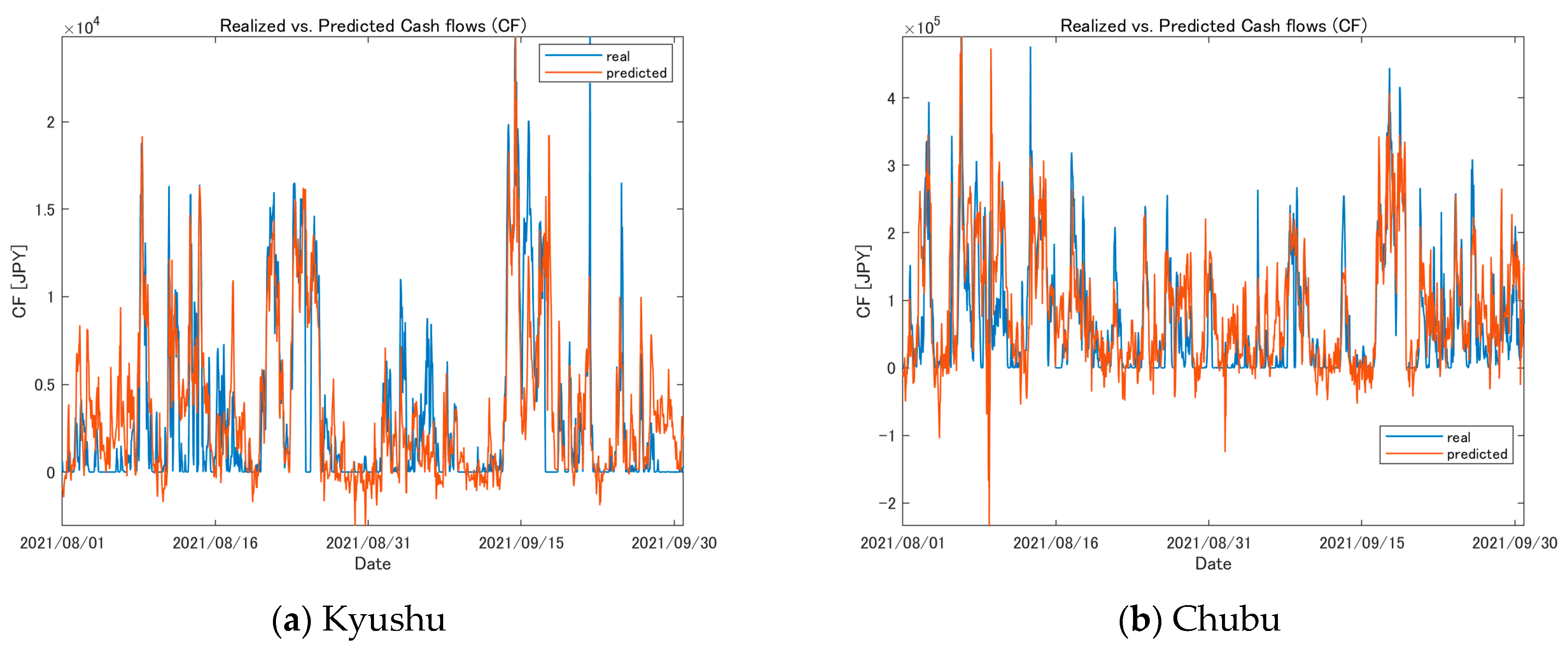
Given the estimated smooth functions and coefficients of (2)–(4), which were obtained using the learning period of data, we can compute the predicted values of the target cash flows in the out-of-sample period by substituting the observed data into the regression equations. Note that such values do not necessarily provide forecasts from the past period because they contain explanatory variables that are measured at the same time as when the target value is observed. However, plotting the predicted values with the realized values of may help us intuitively grasp how hedging is performed in the out-of-sample period.
Panels (a) and (b) in Figure 5 illustrate the realized versus predicted values of for the WFs in Kyushu and Chubu, respectively, during the out-of-sample period. The red lines denote the predicted values of , computed by (4) using lagged and forward variables, whereas the blue lines denote the realized values of . Note that the difference between the red and blue lines provides the hedge errors used to compute the out-of-sample VRR and NMAE in the previous figures. In both cases, the predicted values seem to replicate the realized values in the upward direction but sometimes overshoot or stay away from zero, even though the realized values are zero for some periods. This is because power generation sometimes becomes zero even though the predicted values stay away from zero, which may be a situation where power generation is controlled to be zero to avoid an accident under strong wind. In addition, the target values become zero when the spot electricity price is zero, and this usually occurs when solar generation is large. Both situations are difficult to predict in advance, but it is important to incorporate the effect of unexpected zero values of target cash flows because they may lead to a large loss for wind power generators. This is an interesting topic to explore further in a future work.
4. Hedging with Longer Horizons
In the previous sections, we have assumed to apply hedges at every hour using derivatives with the hourly settlement. The advantage of considering hedging with high frequency is that it enables the hedger to have the flexibility of selecting the time interval and adjusting the hedge ratio when executing derivative contracts. On the other hand, the hedger may consider applying hedges for a longer time horizon or less frequently, e.g., every day or so. In this section, we introduce a hedging problem with a longer horizon (i.e., low-granular hedging) to reduce the fluctuation of daily revenues. Then, we make a comparison with the high-granular hedging developed in the previous sections.
4.1. Daily Hedging Models
Let be a revenue at day given by the sum of hourly revenues as
where stands for a set of 24-hour indexes at day (e.g., ). Similarly, we define the underlying daily indexes related to the wind speed and area-wide wind power production, and , as
For the daily spot electricity price index, we take the average of 24-hour prices at day , i.e.,
With this notation, we introduce the following hedging problem with respect to the daily revenue as
where is a payoff function of the derivative contract and is optimized under the zero-mean condition. Based on a similar argument to that of solving (1), the optimization problem in (10) may be solved by constructing suitable regression equations.
In this study, we construct the following two regression equations, corresponding to linear hedging and spline hedging, respectively:
where denotes a yearly repetitive dummy variable to reflect the seasonality of wind speed in a year, and are cubic spline functions, is a cyclic spline function, and is a residual. The first equation is a linear regression equation, whereas the second may be solved as a GAM to minimize the residual sum of squares with a penalty on smoothness. Then, we obtain linear hedging and spline hedging strategies to solve the optimal hedging problem for the daily setting defined in (10).
As stated in Section 2.3, the cyclic smoothing basis used in the cyclic spline function in (12) enables us to model a periodic function whose endpoint smoothly connects with the initial point (see [51] for the definitions of tensor product and cyclic spline functions). Note that the consideration of wind direction is limited to hourly hedging in this study as it is observed on an hourly basis and poses challenges in defining a representative daily value. Nevertheless, incorporating the influence of wind direction in daily hedging could be a potential avenue for future research by exploring its frequency or other relevant parameters.
The coefficient vector in (11) is estimated as a linear regression problem, whereas spline functions , , and (as well as the intercept ) in (12) are estimated using the GAM given the observed data in the learning period. Note that once the regression problems are solved, the optimal linear payoff function and nonlinear payoff function are given by estimated regression equations in (11) and (12), and the residuals provide (daily) hedging errors. Because there is no wind direction term for the daily hedges, we only have two hedging models, but a seasonal trend is incorporated in (12) in the case of daily hedges.
Another way for deriving daily hedging is to apply hourly hedging consecutively using regression equations in (2)–(4). In this case, the daily hedging errors, denoted by , may be computed by the sum of hourly hedging errors, i.e.,
where is an hourly hedging error when the optimal hedging is performed hourly.
To estimate the daily hedge performance in the out-of-sample case, we compute the VRR and NMAE given as follows, similar to that of the hourly hedges defined in Section 2.4:
where denotes the daily hedge errors in the test period and is replaced by when hourly hedging is applied consecutively to estimate the daily hedge errors.
4.2. Empirical Performance of Daily Hedges
We estimate the optimal regression functions and other required parameters in (11) and (12) using the data in the learning period and apply daily hedging for the out-of-sample data in the test period to evaluate the out-of-sample hedge performance. Similarly, we apply hourly hedging based on the regression Equations (2)–(4) and measure daily hedging errors in the out-of-sample test period. We use the same set of data described in Section 2.5 but consider extending the learning period by sliding the one-year window for the test period as follows (see Appendix A for descriptive statistics of variables):
Period (1) Learning period: 1 October 2019 to 30 September 2020 (Number of daily observations: 366). Test period: 1 October 2020 to 30 September 2021 (Number of daily observations: 365). Kyushu and Chubu.
Period (2) Learning period: 1 October 2019 to 31 March 2021. (Number of daily observations: 548). Test period: 1 April 2021 to 31 March 2022 (Number of daily observations: 365). Kyushu and Chubu.
Period (3) Learning period: 1 October 2019 to 30 September 2021. (Number of daily observations: 731). Test period: 1 October 2021 to 30 September 2022 (Number of daily observations: 365). Kyushu only.
Noting that the data period of the wind farm in Chubu is only until 31 March 2022 (because a portion of the wind farm was separated from the balancing group after 31 March 2022), we performed the empirical test using data in Periods (1)–(3) for the wind farm in Kyushu and in Periods (1) and (2) for the wind farm in Chubu. We examine the hedge effect using VRR and NMAE mainly based on the bar graphs shown in Figure 6 and Figure 7 in this section. Note that the numerical results are listed in table format in Appendix B.
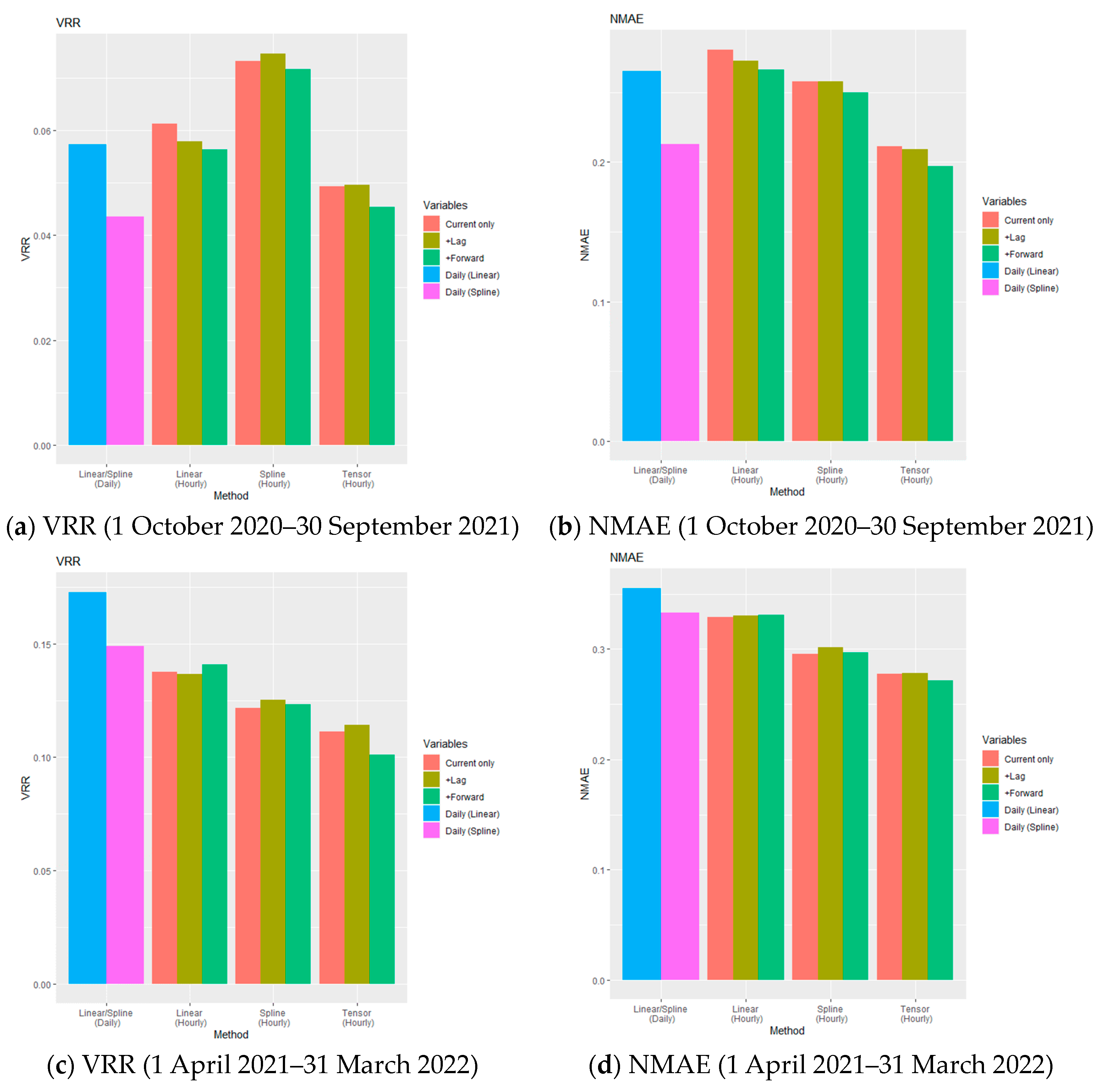
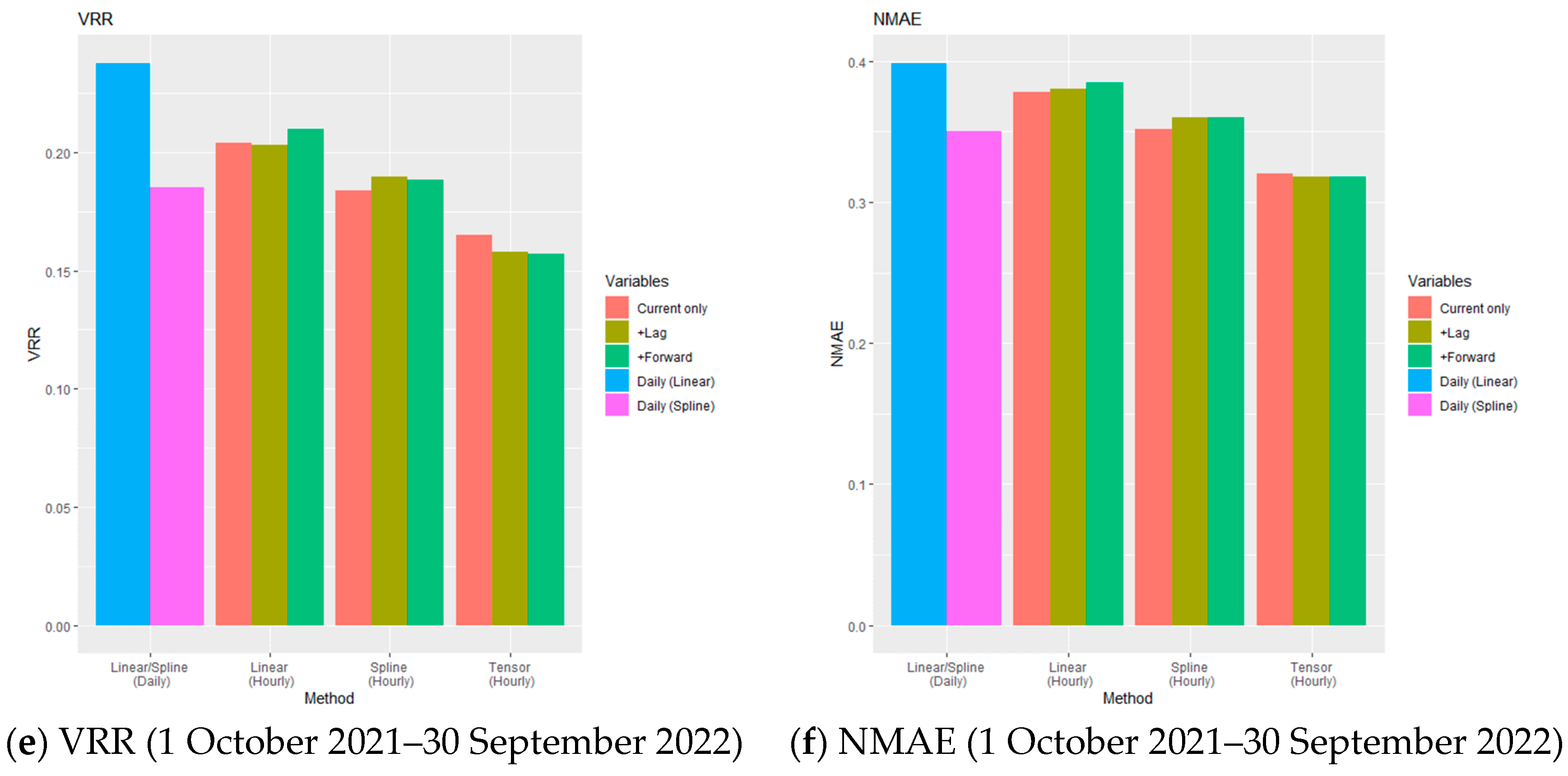
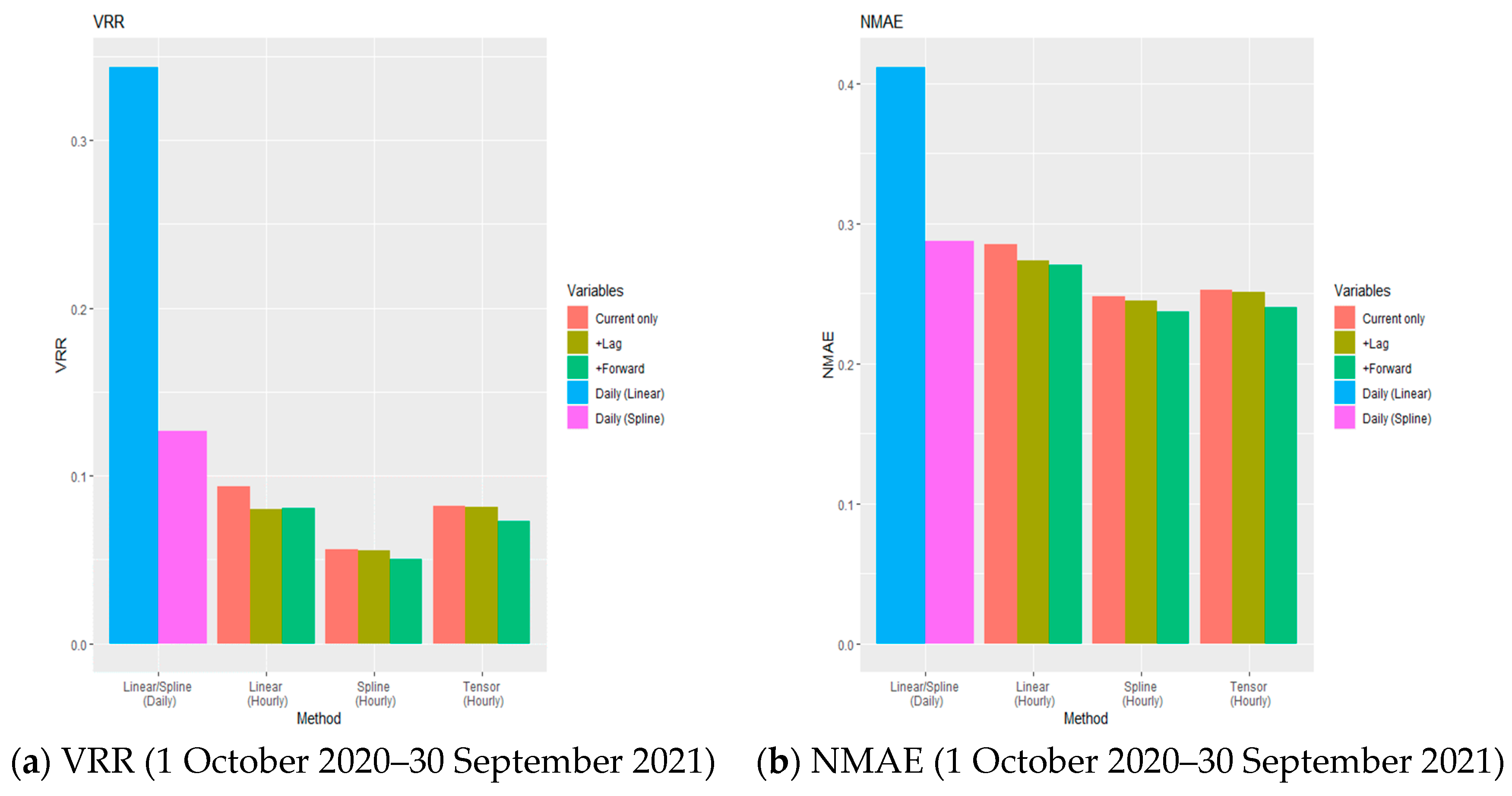
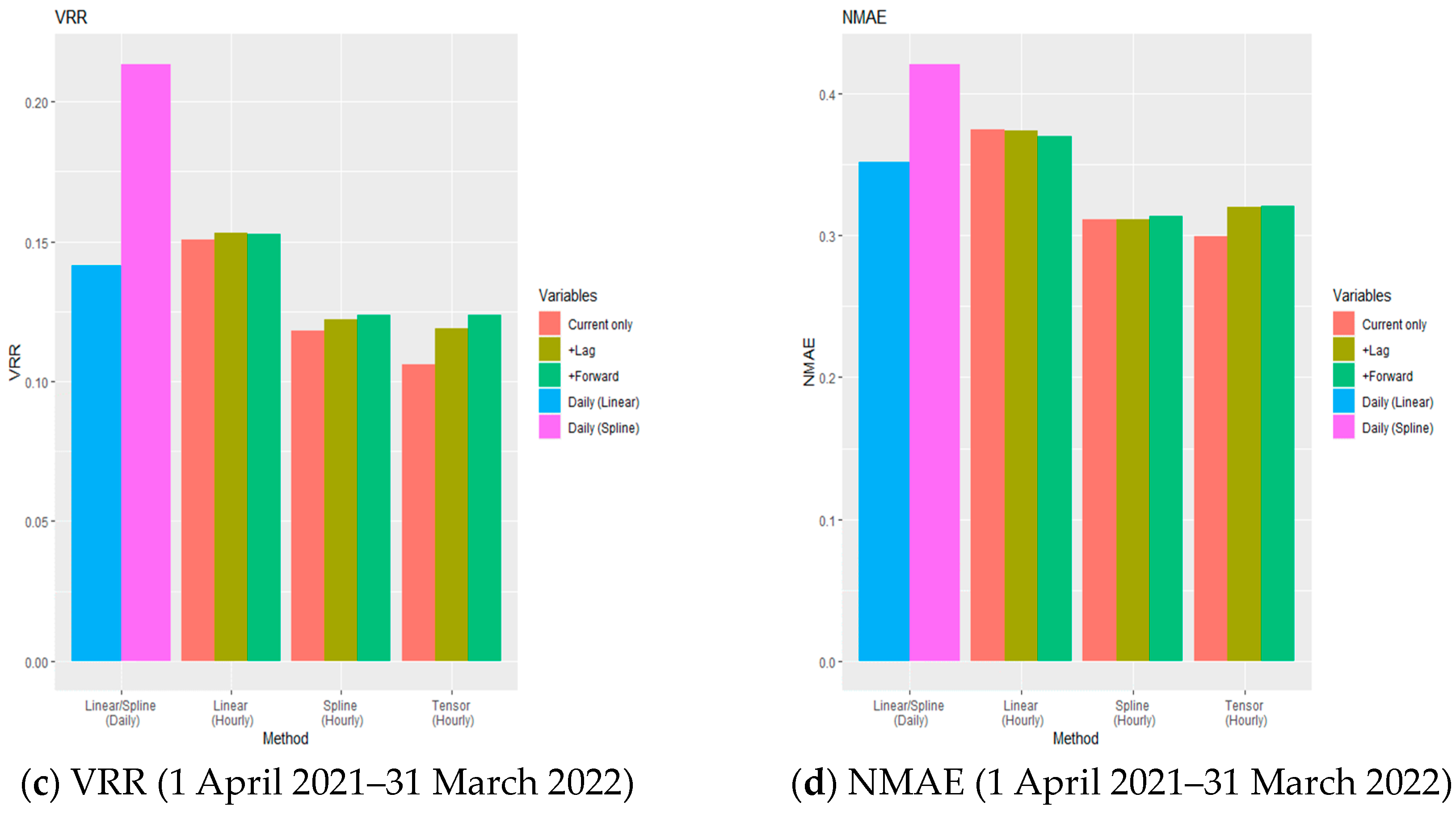
Panels (a), (c), and (e) in Figure 6 illustrate the relationship between the hedge effects estimated by VRR for the out-of-sample periods in Periods (1), (2), and (3), respectively, whereas Panels (b), (d), and (f) illustrate those by NMAE in the corresponding periods. The cyan and magenta bins are estimated by applying (11) and (12), respectively, for the daily observation data, which are labeled as “Linear (Daily)” and “Spline (Daily)”. On the other hand, the rest of the bins are estimated using hourly hedges based on (2)–(4) and are labeled as “Linear (Hourly)”, “Spline (Hourly)”, and “Tensor (Hourly)” on the x-axis, where the three sets of bins compare the VRR and NMAE while incorporating lagged (and forward) variables in addition to current observations as in Figure 3.
At first, we see that nonlinear hedging using the GAM (12) always provided a better hedge performance in terms of both VRR and NMAE than linear hedging using linear regression (11) for all periods. Second, when the rest of the three hedging models are compared, both VRR and NMAE obtained via tensor hedging, i.e., the ones labeled as “Tensor (Hourly)”, demonstrated a tendency to outperform those obtained through the utilization of linear and spline hedging techniques, labeled as “Linear (Hourly)” and “Spline (Hourly)”, respectively; this agrees with the aforementioned results in Section 3 for the hourly hedges. In addition, the effect of lagged and forward variables was not significant for the improvement of VRR and NMAE. Third, if the linear hedging using daily data is compared with the linear hedging using hourly data, the hedge performance tended to be improved when using hourly data or provided no significant difference between the two. A similar tendency was observed for nonlinear hedging, where VRR and NMAE obtained from hedging with hourly data were at least as good as those from hedging with daily data or improved when the hedges with tensor spline functions, i.e., “Tensor (Hourly)”, were applied.
Panels (a)–(d) in Figure 7 provide the results for the wind farm in Chubu when using the data in Periods (1) and (2). Note that there exist certain cases wherein nonlinear hedging does not necessarily exhibit superior performance to linear hedging in Period (2). However, hedging with hourly data showed a better performance at least for “Spline (Hourly)” and “Tensor (Hourly)” compared with both linear and nonlinear hedging using daily data.
In conclusion, our empirical analysis in this section reveals that hedging with the high-granular (hourly) formulation generally provides a better hedge effect than that with the low-granular (daily) formulation and has the advantage of improving the hedge effect.
5. Discussion and Concluding Remarks
In this study, we developed a quantitative strategy for controlling cash flow fluctuations for wind power producers using mixed derivatives on wind indexes and electricity prices. We adopted a flexible approach that optimally synthesizes the payoff function by applying nonparametric regression techniques to reflect the individual wind power generation with fine granularity. An empirical back test was conducted to illustrate our proposed hedging strategy. The out-of-sample simulation results demonstrated that the incorporation of both wind power production and wind weather condition indexes always improved VRR and NMAE, enhancing the value of our high-resolution weather derivatives and the effectiveness of the hedging strategy with mixed derivatives. We also compared the hedge performance between high-granular (hourly) and low-granular (daily) formulations and showed the advantages of utilizing a high-granular hedging formulation for improving the hedge effect.
In addition, the new modeling method using a bivariate tensor product spline function consisting of a wind direction trend with periodicity constraints and a wind speed trend provides a novel perspective in the context of wind power forecasting models, which has attracted much attention in recent years. In wind power forecasting, controlling noise effects and performing a robust model estimation of nonlinear components has been challenging, and various methods have been proposed [54]. Our approach provides a suggestion for this challenge as well.
Finally, we provide supplementary deliberations, encompassing prospective observations.
In the design and trading of derivatives that exhibit high granularity in both temporal and spatial dimensions, it is noteworthy to acknowledge that transaction costs must be taken into account when implementing them in practice. However, the derivatives proposed in this study do not entail payment procedures at the time of contracting and can be calculated relatively easily based solely on historical generation, prices, and weather data, thereby mitigating potential concerns regarding transaction costs. In fact, with the advent of digitalized platforms that support automatic calculations and contracts, the transaction costs are expected to be minimal. While the practical application of such a trading scheme may necessitate further consideration, the rapid advancement of cutting-edge information technology in recent years is anticipated to facilitate the efficient trading of derivatives.
In the policy context of transitioning from FIT to FIP, the significance of price risk hedging is expected to be further accentuated. Furthermore, considering the evolutionary trajectory of the market development, characterized by the advancement of various financial instruments and the changing landscape of decentralized wind power deployment across diverse regions, the issues addressed in this study, namely the need for a sophisticated approach to concurrently manage wind power price and volume risk, as well as the development of such enabling trading environments, are projected to become progressively indispensable in practice. Additionally, with the growing prevalence of variable renewable energy sources, the demand for diversified risk management methods in the electricity market is anticipated to escalate.
As power generators transition towards decentralization, such as local wind and solar power generation, employing finely grained weather indexes may prove to be a more effective strategy for hedging against risks through the utilization of derivative instruments. Considering this situation, the fundamental concepts presented in this study regarding the integration of mixed derivatives that account for both localized and regional indexes, along with the associated technical modeling approaches, are expected to be further developed and investigated, including their applicability to other domains within the power sector.
Author Contributions
Conceptualization, Y.Y. and T.M.; data curation, Y.Y.; formal analysis, Y.Y.; funding acquisition, Y.Y. and T.M.; investigation, Y.Y. and T.M.; methodology, Y.Y. and T.M.; project administration, Y.Y.; resources, Y.Y.; software, Y.Y.; supervision, Y.Y.; validation, Y.Y.; visualization, Y.Y.; writing—original draft, Y.Y.; writing—review and editing, Y.Y. and T.M. All authors have read and agreed to the published version of the manuscript.
Funding
Grant-in-Aid for Scientific Research (A) 20H00285, Grant-in-Aid for Challenging Research (Exploratory) 19K22024, and Grant-in-Aid for Young Scientists 21K14374 from the Japan Society for the Promotion of Science (JSPS).
Data Availability Statement
The JEPX spot prices, WPP indexes for Kyushu and Chubu, and weather data used in this study were obtained from the following websites: https://www.kyuden.co.jp/td_service_wheeling_rule-document_disclosure (accessed on 19 March 2023); https://powergrid.chuden.co.jp/denkiyoho/ (accessed on 19 March 2023); and https://www.data.jma.go.jp/gmd/risk/obsdl/ (accessed on 19 March 2023). The power generation data of the WFs located in the Kyushu and Chubu areas, Japan, were provided by UPDATER Co., Ltd. (Tokyo, Japan) and are available from the first author upon reasonable request.
Acknowledgments
This work was supported by Grant-in-Aid for Scientific Research (A) 20H00285, Grant-in-Aid for Challenging Research (Exploratory) 19K22024, and Grant-in-Aid for Young Scientists 21K14374 from the Japan Society for the Promotion of Science (JSPS). We express our sincere gratitude to UPDATER Co., Ltd. (Tokyo, Japan) for providing the power generation data for the wind farms.
Conflicts of Interest
The authors declare no conflict of interest.
Nomenclature
| The power output of a WF | |
| Spot electricity price | |
| Wind speed | |
| Wind direction | |
| Area-wide wind power generation | |
| Wind power generation indexes | |
| Wind weather condition indexes | |
| Hedging errors | |
| Cubic spline function | |
| Bivariate tensor product spline function | |
| Coefficient vector | |
| VRR | Variance reduction rates |
| NMAE | Normalized mean absolute errors |
| Note: The subscripts and are omitted in the above list, where and stand for hour and day, respectively. Moreover, variables, functions, and indexes for date granularity data are denoted with a hat in the text. | |
Appendix A. Descriptive Statistics of Variables for Hourly Hedging
In this appendix, we demonstrate the descriptive statistics of variables used for the hourly and daily hedging performed in Section 3 and Section 4. Table A1 and Table A2 show the descriptive statistics of the hourly data in Kyushu and Chubu, respectively, for the learning and test periods, whereas Table A3 and Table A4 displays those of the daily data in Kyushu and Chubu, respectively. Note that, for daily data, only the case of Period (1) is shown.

Table A1.
Descriptive statistics of hourly data in Kyushu for learning and test periods.
| WF Generation [kWh] | Spot Price [JPY/kWh] | Cash Flow [JPY] | WPP Index [MWh] | W1 [m/s] | W2 [m/s] | |
|---|---|---|---|---|---|---|
| Learning period | ||||||
| Mean | 544 | 5.63 | 78.2 | 2.93 | 3.94 | |
| SD | 626 | 3.81 | 74.3 | 1.88 | 2.43 | |
| Min | 0.00 | 0.01 | 0.00 | 0.00 | 0.00 | 0.00 |
| Max | 50.2 | 361 | 19.7 | 28.8 | ||
| Test period | ||||||
| Mean | 650 | 22.7 | 80.8 | 1.81 | 2.33 | |
| SD | 567 | 11.8 | 90.9 | 2.87 | 4.00 | |
| Min | 0.00 | 0.01 | 0 | 0 | 0 | 0 |
| Max | 235 | 370 | 12.5 | 16.8 | ||
Learning period: 1 October 2019 to 30 September 2020; test period: 1 October 2020 to 30 September 2021. WF generation: power generation of WF in Kyushu [kWh]; spot price: area price in Kyushu (hourly average) [JPY]; cash flow: cash flow of WF [JPY]; WPP index: area-wide wind power generation data in Kyushu [MWh]; W1,W2: wind speeds observed at two meteorological weather stations near the WF [m/s].
Table A2.
Descriptive statistics of hourly data in Chubu for learning and test periods.
| WF Generation [kWh] | Spot Price [JPY/kWh] | Cash Flow [JPY] | WPP Index [MWh] | W1 [m/s] | W2 [m/s] | W3 [m/s] | W4 [m/s] | |
|---|---|---|---|---|---|---|---|---|
| Learning period | ||||||||
| Mean | 6.03 | 59.3 | 1.42 | 2.58 | 1.53 | 2.27 | ||
| SD | 3.82 | 52.8 | 1.15 | 1.70 | 1.20 | 1.78 | ||
| Min | 0.00 | 0.01 | 0.00 | 0.00 | 0.00 | 0.00 | 0.00 | 0.00 |
| Max | 50.2 | 237 | 11.3 | 12.6 | 9.90 | 12.3 | ||
| Test period | ||||||||
| Mean | 12.3 | 63.3 | 1.32 | 2.54 | 1.49 | 2.13 | ||
| SD | 22.4 | 57.4 | 1.06 | 1.72 | 1.20 | 1.69 | ||
| Min | 0.00 | 0.01 | 0.00 | 0.00 | 0.00 | 0.00 | 0.00 | 0.00 |
| Max | 235 | 239 | 7.80 | 11.2 | 9.30 | 9.90 | ||
Learning period: 1 October 2019 to 30 September 2020; test period: 1 October 2020 to 30 September 2021. WF generation: power generation of WF in Chubu [kWh]; spot price: area price in Kyushu (hourly average) [JPY]; cash flow: cash flow of WF [JPY]; WPP index: area-wide wind power generation data in Kyushu [MWh]; W1–W4: wind speeds observed at four meteorological weather stations near the WF [m/s].
Table A3.
Descriptive statistics of daily data in Kyushu for learning and test periods.
| WF Generation [kWh] | Spot Price [JPY/kWh] | Cash Flow [JPY] | WPP Index [MWh] | W1 [m/s] | W2 [m/s] | |
|---|---|---|---|---|---|---|
| Learning period | ||||||
| Mean | 5.63 | 78.2 | 2.93 | 3.94 | ||
| SD | 2.18 | 62.1 | 1.33 | 1.76 | ||
| Min | 0.00 | 2.10 | 0.00 | 0.792 | 1.07 | 1.42 |
| Max | 17.2 | 302 | 11.2 | 12.3 | ||
| Test period | ||||||
| Mean | 11.8 | 90.9 | 2.87 | 4.00 | ||
| SD | 19.8 | 70.0 | 1.31 | 1.77 | ||
| Min | 0.00 | 3.06 | 0.00 | 1.04 | 0.992 | 1.13 |
| Max | 140 | 305 | 7.55 | 11.0 | ||
Learning period: 1 October 2019 to 30 September 2020; test period: 1 October 2020 to 30 September 2021. WF generation: total daily power generation of WF in Kyushu [kWh]; spot price: area price in Kyushu (daily average) [JPY]; cash flow: total daily cash flow of WF [JPY]; WPP index: area-wide wind power generation data in Kyushu (daily average) [MWh]; W1,W2: wind speeds observed at two meteorological weather stations near the WF (daily average) [m/s].
Table A4.
Descriptive statistics of daily data in Chubu for learning and test periods.
| WF Generation [kWh] | Spot Price [JPY/kWh] | Cash Flow [JPY] | WPP Index [MWh] | W1 [m/s] | W2 [m/s] | W3 [m/s] | W4 [m/s] | |
|---|---|---|---|---|---|---|---|---|
| Learning period | ||||||||
| Mean | 6.03 | 59.3 | 1.42 | 2.58 | 1.53 | 2.27 | ||
| SD | 2.36 | 44.6 | 0.810 | 1.15 | 0.679 | 1.18 | ||
| Min | 0.00 | 2.10 | 0.00 | 2.29 | 0.367 | 0.971 | 0.429 | 0.671 |
| Max | 17.4 | 196 | 5.35 | 8.01 | 4.11 | 6.43 | ||
| Test period | ||||||||
| Mean | 12.3 | 63.3 | 1.32 | 2.54 | 1.49 | 2.13 | ||
| SD | 19.3 | 50.3 | 0.705 | 1.15 | 0.698 | 1.08 | ||
| Min | 3.07 | 1.04 | 0.279 | 1.01 | 0.458 | 0.504 | ||
| Max | 132 | 206 | 3.85 | 7.30 | 4.19 | 6.23 | ||
Learning period: 1 October 2019 to 30 September 2020; test period: 1 October 2020 to 30 September 2021. WF generation: total daily power generation of the WF in Chubu [kWh]; spot price: area price Chubu (daily average) [JPY]; cash flow: total daily cash flow of WF [JPY]; WPP index: area-wide wind power generation data in Kyushu (daily average) [MWh]; W1–W4: wind speeds observed at four meteorological weather stations near WF (daily average) [m/s].
Appendix B. Numerical Results for VRR and NMAE
In Section 3 and Section 4, we conducted a comprehensive analysis of the hedge effect of our proposed methodologies, employing VRR and NMAE as the primary evaluation metrics, predominantly based on the analysis of bar graphs from Figure 3, Figure 4, Figure 6 and Figure 7. In this appendix, we arrange the numerical results in tabular formats to present their actual values in Table A5, Table A6, Table A7, Table A8, Table A9 and Table A10 below.
Table A5.
Out-of-sample VRR and NMAE vs. in-sample cases with the comparison for the effect of lagged and forward variables (Kyushu; see bar graphs in Figure 3).
Table A5.
Out-of-sample VRR and NMAE vs. in-sample cases with the comparison for the effect of lagged and forward variables (Kyushu; see bar graphs in Figure 3).
| VRR (Current only) | VRR (+Lag) | VRR (+Forward) | NMAE (Current only) | NMAE (+Lag) | NMAE (+Forward) | |
|---|---|---|---|---|---|---|
| In-sample | ||||||
| Linear | 11.5% | 11.4% | 9.7% | 32.8% | 32.8% | 31.2% |
| Spline | 10.9% | 10.6% | 8.9% | 33.1% | 33.4% | 31.8% |
| Tensor | 9.4% | 8.9% | 7.0% | 29.9% | 30.3% | 27.9% |
| Out-of-sample | ||||||
| Linear | 21.2% | 20.1% | 19.4% | 42.1% | 41.3% | 40.1% |
| Spline | 14.9% | 15.0% | 13.6% | 35.9% | 35.9% | 34.4% |
| Tensor | 12.5% | 13.1% | 11.4% | 32.1% | 32.1% | 30.2% |
Learning period: 1 October 2019 to 30 September 2020; test period: 1 October 2020 to 30 September 2021.
Table A6.
Out-of-sample VRR and NMAE vs. in-sample cases with the comparison for the effect of lagged and forward variables (Chubu; see bar graphs in Figure 3).
Table A6.
Out-of-sample VRR and NMAE vs. in-sample cases with the comparison for the effect of lagged and forward variables (Chubu; see bar graphs in Figure 3).
| VRR (Current only) | VRR (+Lag) | VRR (+Forward) | NMAE (Current only) | NMAE (+Lag) | NMAE (+Forward) | |
|---|---|---|---|---|---|---|
| In-sample | ||||||
| Linear | 18.3% | 17.2% | 16.6% | 42.7% | 42.1% | 41.7% |
| Spline | 16.9% | 15.9% | 14.8% | 41.3% | 41.3% | 41.2% |
| Tensor | 13.4% | 10.7% | 8.3% | 40.6% | 40.4% | 39.0% |
| Out-of-sample | ||||||
| Linear | 22.9% | 21.9% | 22.6% | 45.8% | 45.0% | 45.5% |
| Spline | 19.6% | 19.3% | 19.1% | 42.7% | 42.2% | 42.2% |
| Tensor | 22.0% | 20.8% | 19.3% | 42.5% | 42.0% | 40.9% |
Learning period: 1 October 2019 to 30 September 2020; test period: 1 October 2020 to 30 September 2021.
Table A7.
Out-of-sample VRR and NMAE vs. in-sample cases with the comparison for the effect of the incorporation of the WPP or WWC index (Kyushu; see bar graphs in Figure 4).
Table A7.
Out-of-sample VRR and NMAE vs. in-sample cases with the comparison for the effect of the incorporation of the WPP or WWC index (Kyushu; see bar graphs in Figure 4).
| VRR (w/WPP) | VRR (w/WWC) | VRR (w/WPP and WWC) | NMAE (w/WPP) | NMAE (w/WWC) | NMAE (w/WPP and WWC) | |
|---|---|---|---|---|---|---|
| In-sample | ||||||
| Linear | 17.9% | 14.5% | 9.7% | 42.6% | 35.8% | 31.2% |
| Spline | 15.7% | 14.5% | 8.9% | 42.9% | 35.9% | 31.8% |
| Tensor | 15.7% | 10.4% | 7.1% | 42.9% | 30.8% | 28.0% |
| Out-of-sample | ||||||
| Linear | 22.2% | 51.2% | 19.4% | 45.9% | 55.9% | 40.1% |
| Spline | 19.5% | 24.4% | 13.6% | 44.3% | 42.8% | 34.4% |
| Tensor | 19.5% | 18.3% | 11.5% | 44.3% | 35.5% | 30.3% |
Learning period: 1 October 2019 to 30 September 2020; test period: 1 October 2020 to 30 September 2021.
Table A8.
Out-of-sample VRR and NMAE vs. in-sample cases with the comparison for the effect of the incorporation of the WPP or WWC index (Chubu; see bar graphs Figure 4).
Table A8.
Out-of-sample VRR and NMAE vs. in-sample cases with the comparison for the effect of the incorporation of the WPP or WWC index (Chubu; see bar graphs Figure 4).
| VRR (w/WPP) | VRR (w/WWC) | VRR (w/WPP and WWC) | NMAE (w/WPP) | NMAE (w/WWC) | NMAE (w/WPP and WWC) | |
|---|---|---|---|---|---|---|
| In-sample | ||||||
| Linear | 22.8% | 24.2% | 16.6% | 46.0% | 50.4% | 41.7% |
| Spline | 21.1% | 22.3% | 14.8% | 43.0% | 49.4% | 41.2% |
| Tensor | 21.1% | 12.3% | 8.3% | 43.0% | 46.5% | 39.2% |
| Out-of-sample | ||||||
| Linear | 28.7% | 30.6% | 22.6% | 51.3% | 51.9% | 45.5% |
| Spline | 24.2% | 29.3% | 19.1% | 47.1% | 50.4% | 42.2% |
| Tensor | 24.2% | 23.3% | 18.2% | 47.1% | 43.5% | 39.8% |
Learning period: 1 October 2019 to 30 September 2020; test period: 1 October 2020 to 30 September 2021.
Table A9.
Comparison of daily hedges with hourly hedges (Kyushu; see bar graphs in Figure 6).
Table A9.
Comparison of daily hedges with hourly hedges (Kyushu; see bar graphs in Figure 6).
| VRR (Current only) | VRR (+Lag) | VRR (+Forward) | NMAE (Current only) | NMAE (+Lag) | NMAE (+Forward) | |
|---|---|---|---|---|---|---|
| Period (1) | ||||||
| Linear (Hourly) | 6.1% | 5.8% | 5.6% | 28.1% | 27.3% | 26.7% |
| Spline (Hourly) | 7.3% | 7.5% | 7.2% | 25.8% | 25.8% | 25.0% |
| Tensor (Hourly) | 4.9% | 5.0% | 4.5% | 21.1% | 20.9% | 19.7% |
| Period (2) | ||||||
| Linear (Hourly) | 13.7% | 13.6% | 14.1% | 32.9% | 33.1% | 33.1% |
| Spline (Hourly) | 12.2% | 12.5% | 12.3% | 29.6% | 30.2% | 29.7% |
| Tensor (Hourly) | 11.1% | 11.4% | 10.1% | 27.7% | 27.8% | 27.2% |
| Period (3) | ||||||
| Linear (Hourly) | 20.4% | 20.3% | 21.0% | 37.8% | 38.1% | 38.5% |
| Spline (Hourly) | 18.4% | 19.0% | 18.8% | 35.2% | 36.0% | 36.0% |
| Tensor (Hourly) | 16.5% | 15.8% | 15.7% | 32.0% | 31.8% | 31.8% |
| VRR Period (1) | NMAE Period (1) | VRR Period (2) | NMAE Period (2) | VRR Period (3) | NMAE Period (3) | |
| Linear (Daily) | 5.7% | 26.5% | 17.3% | 35.5% | 23.8% | 39.9% |
| Spline (Daily) | 4.4% | 21.3% | 14.9% | 33.3% | 18.5% | 35.0% |
Table A10.
Comparison of daily hedges with hourly hedges (Chubu; see bar graphs in Figure 7).
Table A10.
Comparison of daily hedges with hourly hedges (Chubu; see bar graphs in Figure 7).
| VRR (Current only) | VRR (+Lag) | VRR (+Forward) | NMAE (Current only) | NMAE (+Lag) | NMAE (+Forward) | |
|---|---|---|---|---|---|---|
| Period (1) | ||||||
| Linear (Hourly) | 9.4% | 8.0% | 8.1% | 28.5% | 27.4% | 27.1% |
| Spline (Hourly) | 5.6% | 5.5% | 5.0% | 24.8% | 24.5% | 23.7% |
| Tensor (Hourly) | 8.2% | 8.1% | 7.3% | 25.2% | 25.1% | 24.0% |
| Period (2) | ||||||
| Linear (Hourly) | 15.1% | 15.3% | 15.3% | 37.5% | 37.4% | 37.0% |
| Spline (Hourly) | 11.8% | 12.2% | 12.4% | 31.1% | 31.2% | 31.3% |
| Tensor (Hourly) | 10.6% | 11.9% | 12.4% | 30.0% | 32.0% | 32.1% |
| VRR Period (1) | NMAE Period (1) | VRR Period (2) | NMAE Period (2) | |||
| Linear (Daily) | 34.4% | 41.2% | 14.1% | 35.2% | ||
| Spline (Daily) | 12.7% | 28.7% | 21.3% | 42.1% | ||
References
- Deng, S.J.; Oren, S.S. Electricity derivatives and risk management. Energy 2006, 31, 940–953. [Google Scholar] [CrossRef]
- Brockett, P.L.; Wang, M.; Yang, C. Weather derivatives and weather risk management. Risk Manag. Insur. Rev. 2005, 8, 127–140. [Google Scholar] [CrossRef]
- Halkos, G.E.; Tsirivis, A.S. Energy commodities: A review of optimal hedging strategies. Energies 2019, 12, 3979. [Google Scholar] [CrossRef]
- Eydeland, A.; Wolyniec, K. Energy and Power risk Management: New Developments in Modeling, Pricing, and Hedging; John Wiley & Sons, Ltd.: Hoboken, NJ, USA, 2002; Volume 97. [Google Scholar]
- Clewlow, L.; Strickland, C. Energy Derivatives: Pricing and Risk Management; Lacima: Sydney, NS, Australia, 2000. [Google Scholar]
- Wieczorek-Kosmala, M. Weather risk management in energy sector: The Polish case. Energies 2020, 13, 945. [Google Scholar] [CrossRef]
- Alexandridis, A.K.; Zapranis, A.D. Weather Derivatives, Modeling and Pricing Weather-Related Risk; Springer: New York, NY, USA, 2013; ISBN 978-1-4614-6070-1. [Google Scholar]
- Burger, M.; Klar, B.; Muller, A.; Schindlmayr, G.A. spot market model for pricing derivatives in electricity markets. Quant. Financ. 2004, 4, 109–122. [Google Scholar] [CrossRef]
- Jewson, S.; Brix, A. Weather Derivative Valuation: The Meteorological, Statistical, Financial and Mathematical Foundations; Cambridge University Press: Cambridge, UK, 2005; p. 392. [Google Scholar]
- Roncoroni, A.; Fusai, G.; Cummins, M. Handbook of Multi-Commodity Markets and Products: Structuring, Trading and Risk Management; John Wiley & Sons, Ltd.: Hoboken, NJ, USA, 2015; pp. 255–277. [Google Scholar]
- Berhane, T.; Shibabaw, A.; Awgichew, G.; Walelgn, A. Pricing of weather derivatives based on temperature by obtaining market risk factor from historical data. Model. Earth Syst. Environ. 2021, 7, 871–884. [Google Scholar] [CrossRef]
- Elias, R.S.; Wahab, M.I.M.; Fang, L. A comparison of regime-switching temperature modeling approaches for applications in weather derivatives. Eur. J. Oper. Res. 2014, 232, 549–560. [Google Scholar] [CrossRef]
- Zapranis, A.; Alexandridis, A. Modelling the temperature time-dependent speed of mean reversion in the context of weather derivatives pricing. Appl. Math. Financ. 2008, 15, 355–386. [Google Scholar] [CrossRef]
- Benth, F.E.; Benth, J.Š. The volatility of temperature and pricing of weather derivatives. Quant. Financ. 2007, 7, 553–561. [Google Scholar] [CrossRef]
- Gyamerah, S.A.; Ngare, P.; Ikpe, D. Hedging Crop Yields Against Weather Uncertainties—A Weather Derivative Perspective. Math. Comput. Appl. 2019, 24, 71. [Google Scholar] [CrossRef]
- Alaton, P.; Djehiche, B.; Stillberger, D. On modelling and pricing weather derivatives. Appl. Math. Financ. 2002, 9, 1–20. [Google Scholar] [CrossRef]
- Boyle, C.F.; Haas, J.; Kern, J.D. Development of an irradiance-based weather derivative to hedge cloud risk for solar energy systems. Renew. Energy 2021, 164, 1230–1243. [Google Scholar] [CrossRef]
- Mosquera-López, S.; Uribe, J.M. Pricing the risk due to weather conditions in small variable renewable energy projects. Appl. Energy 2022, 322, 119476. [Google Scholar] [CrossRef]
- Leobacher, G.; Ngare, P. On modelling and pricing rainfall derivatives with seasonality. Appl. Math. Financ. 2011, 18, 71–91. [Google Scholar] [CrossRef]
- Benth, F.E.; Di Persio, L.; Lavagnini, S. Stochastic modeling of wind derivatives in energy markets. Risks 2018, 6, 56. [Google Scholar] [CrossRef]
- Xiao, Y.; Wang, X.; Wang, X.; Wu, Z. Trading wind power with barrier option. Appl. Energy 2016, 182, 232–242. [Google Scholar] [CrossRef]
- Rodríguez, Y.E.; Pérez-Uribe, M.A.; Contreras, J. Wind put barrier options pricing based on the Nordix index. Energies 2021, 14, 1177. [Google Scholar] [CrossRef]
- Masala, G.; Micocci, M.; Rizk, A. Hedging Wind Power Risk Exposure through Weather Derivatives. Energies 2022, 15, 1343. [Google Scholar] [CrossRef]
- Kanamura, T.; Homann, L.; Prokopczuk, M. Pricing analysis of wind power derivatives for renewable energy risk management. Appl. Energy 2021, 304, 117827. [Google Scholar] [CrossRef]
- Christensen, T.S.; Pircalabu, A. On the spatial hedging effectiveness of German wind power futures for wind power generators. J. Energy Mark. 2018, 11, 71–96. [Google Scholar] [CrossRef]
- Benth, F.E.; Pircalabu, A. A non-Gaussian Ornstein–Uhlenbeck model for pricing wind power futures. Appl. Math. Financ. 2018, 25, 36–65. [Google Scholar] [CrossRef]
- Gersema, G.; Wozabal, D. An equilibrium pricing model for wind power futures. Energy Econ. 2017, 65, 64–74. [Google Scholar] [CrossRef]
- Thomaidis, N.S.; Christodoulou, T.; Santos-Alamillos, F.J. Handling the risk dimensions of wind energy generation. Appl. Energy 2023, 339, 120925. [Google Scholar] [CrossRef]
- Oum, Y.; Oren, S.; Deng, S. Hedging quantity risks with standard power options in a competitive wholesale electricity market. Nav. Res. Logist. 2006, 53, 697–712. [Google Scholar] [CrossRef]
- Oum, Y.; Oren, S. VaR constrained hedging of fixed Price load-following obligations in competitive electricity markets. J. Risk Decision Anal. 2009, 1, 43–56. [Google Scholar] [CrossRef]
- Oum, Y.; Oren, S. Optimal static hedging of volumetric risk in a competitive wholesale electricity market. Decis. Anal. 2010, 7, 107–122. [Google Scholar] [CrossRef]
- Yamada, Y. Valuation and hedging of weather derivatives on monthly average temperature. J. Risk 2007, 10, 101–125. [Google Scholar] [CrossRef]
- Yamada, Y. Optimal Hedging of Prediction Errors Using Prediction Errors. Asia Pac. Financ. Mark. 2008, 15, 67–95. [Google Scholar] [CrossRef]
- Matsumoto, T.; Yamada, Y. Simultaneous hedging strategy for price and volume risks in electricity businesses using energy and weather derivatives. Energy Econ. 2021, 95, 105101. [Google Scholar] [CrossRef]
- Matsumoto, T.; Yamada, Y. Customized yet Standardized temperature derivatives: A non-parametric approach with suitable basis selection for ensuring robustness. Energies 2021, 14, 3351. [Google Scholar] [CrossRef]
- Yamada, Y.; Matsumoto, T. Going for Derivatives or Forwards? Minimizing Cashflow Fluctuations of Electricity Transactions on Power Markets. Energies 2021, 14, 7311. [Google Scholar] [CrossRef]
- Matsumoto, T.; Yamada, Y. Improving the Efficiency of Hedge Trading Using High-er-Order Standardized Weather Derivatives for Wind Power. Energies 2023, 16, 3112. [Google Scholar] [CrossRef]
- Coulon, M.; Powell, W.B.; Sircar, R. A model for hedging load and price risk in the Texas electricity market. Energy Econ. 2013, 40, 976–988. [Google Scholar] [CrossRef]
- Bhattacharya, S.; Gupta, A.; Kar, K.; Owusu, A. Risk management of renewable power producers from co-dependencies in cashflows. Eur. J. Oper. Res. 2020, 283, 1081–1093. [Google Scholar] [CrossRef]
- Kaufmann, J.; Kienscherf, P.A.; Ketter, W. Modeling and managing joint price and volumetric risk for volatile electricity portfolios. Energies 2020, 13, 3578. [Google Scholar] [CrossRef]
- Benth, F.E.; Lange, N.; Myklebust, T.A. Pricing and hedging quanto options in energy markets. J. Energy Mark. 2015, 8, 1–35. [Google Scholar] [CrossRef]
- Caporin, M.; Preś, J.; Torro, H. Model based Monte Carlo pricing of energy and temperature quanto options. Energy Econ. 2012, 34, 1700–1712. [Google Scholar] [CrossRef]
- Ministry of Economy, Trade and Industry; METI. Present Status and Promotion Measures for the Introduction of Renewable Energy in Japan. 2011. Available online: https://www.meti.go.jp/english/policy/energy_environment/renewable/index.html (accessed on 17 March 2023).
- Nasdaq. Wind Power Futures Based on the German Wind Index NAREX WIDE. 2023. Available online: https://www.nasdaq.com/solutions/wind-power-futuresl (accessed on 17 March 2023).
- Japan Electric Power Information Center, Inc.; JEPIC. The Electric Power Industry in Japan. 2022. Available online: https://en.wikipedia.org/wiki/Feed-in_premium (accessed on 17 March 2023).
- Betz, A. Wind-Energie und ihre Ausnutzung durch Windmühlen; Vandenhoek and Ruprecht: Göttingen, Germany, 1926; 64p. [Google Scholar]
- Villanueva, D.; Feijóo, A. Wind power distributions: A review of their applications. Renew. Sustain. Energy Rev. 2010, 14, 1490–1495. [Google Scholar] [CrossRef]
- Hanifi, S.; Liu, X.; Lin, Z.; Lotfian, S. A critical review of wind power forecasting methods—Past, present and future. Energies 2020, 13, 3764. [Google Scholar] [CrossRef]
- Wood, S.N. Package ‘mgcv’ v. 1.8–42. 2023. Available online: https://cran.r-project.org/web/packages/mgcv/mgcv.pdf (accessed on 25 March 2023).
- Hastie, T.; Tibshirani, R. Generalized Additive Models; Chapman & Hall: Boca Raton, FL, USA, 1990. [Google Scholar]
- Wood, S.N. Generalized Additive Models: An Introduction with R, 2nd ed.; Chapman and Hall: New York, NY, USA, 2017. [Google Scholar]
- Wood, S.N.; Goude, Y.; Fasiolo, M. Interpretability in Generalized Additive Models. In Interpretability for Industry 4.0: Statistical and Machine Learning Approaches; Springer: Cham, Switzerland, 2022. [Google Scholar]
- Matsumoto, T.; Yamada, Y. Comprehensive and Comparative Analysis of GAM-Based PV Power Forecasting Models Using Multidimensional Tensor Product Splines against Machine Learning Techniques. Energies 2021, 14, 7146. [Google Scholar] [CrossRef]
- Liu, H.; Chen, C. Data processing strategies in wind energy forecasting models and applications: A comprehensive review. Appl. Energy 2019, 249, 392–408. [Google Scholar]
Figure 1.
Historical data of the Kyushu area spot electricity price (Panel (a)), WF power generation with the WPP index (Panel (b)), and wind speed data observed at two meteorological weather stations (Panel (c)) during the two months of the data period (i.e., 1 August–30 September 2021).
Figure 1.
Historical data of the Kyushu area spot electricity price (Panel (a)), WF power generation with the WPP index (Panel (b)), and wind speed data observed at two meteorological weather stations (Panel (c)) during the two months of the data period (i.e., 1 August–30 September 2021).

Figure 2.
Estimated tensor spline functions (Panels (a,b)) and univariate spline function (Panel (c)) when regression Equation (4) is applied for the learning period of the data to hedge the cash flow fluctuation of the WF in Kyushu. Note that because there are two observation points of WCC indexes in the case of the WF in Kyushu, two tensor spline functions (Panels (a,b)) and one univariate spline function (Panel (c)) were estimated.

Figure 3.
Out-of-sample VRR and NMAE vs. in-sample cases with the comparison for the effect of lagged and forward variables (see Table A5 and Table A6 in Appendix B for the numerical results). Panel (a)—VRR for the WF in Kyushu. Panel (b)—VRR for the WF in Chubu. Panel (c)—NMAE for the WF in Kyushu. Panel (d)—NMAE for the WF in Chubu.


Figure 4.
Out-of-sample VRR and NMAE vs. in-sample cases with the comparison for the effect of the incorporation of the WPP or WWC index (see Table A7 and Table A8 in Appendix B for the numerical results). Panel (a)—VRR for the WF in Kyushu. Panel (b)—VRR for the WF in Chubu. Panel (c)—NMAE for the WF in Kyushu. Panel (d)—NMAE for the WF in Chubu.

Figure 5.
Realized vs. predicted values of in the out-of-sample period.

Figure 6.
Comparison of daily hedges with hourly hedges in Kyushu (see Table A9 in Appendix B for the numerical results). Panels (a,b): VRR and NMAE for the out-of-sample period of 1 October 2020–30 September 2021. Panels (c,d): VRR and NMAE for the out-of-sample period of 1 April 2021–31 March 2022. Panels (e,f): VRR and NMAE for the out-of-sample period of 1 October 2021–30 September 2022.


Figure 7.
Comparison of daily hedges with hourly hedges in Chubu (see Table A10 in Appendix B for the numerical results). Panels (a,b): VRR and NMAE for the out-of-sample period of 1 October 2020–30 September 2021. Panels (c,d): VRR and NMAE for the out-of-sample period of 1 April 2021–31 March 2022.


Disclaimer/Publisher’s Note: The statements, opinions and data contained in all publications are solely those of the individual author(s) and contributor(s) and not of MDPI and/or the editor(s). MDPI and/or the editor(s) disclaim responsibility for any injury to people or property resulting from any ideas, methods, instructions or products referred to in the content. |
© 2023 by the authors. Licensee MDPI, Basel, Switzerland. This article is an open access article distributed under the terms and conditions of the Creative Commons Attribution (CC BY) license (https://creativecommons.org/licenses/by/4.0/).
Share and Cite
MDPI and ACS Style
Yamada, Y.; Matsumoto, T. Construction of Mixed Derivatives Strategy for Wind Power Producers. Energies 2023, 16, 3809. https://doi.org/10.3390/en16093809
AMA Style
Yamada Y, Matsumoto T. Construction of Mixed Derivatives Strategy for Wind Power Producers. Energies. 2023; 16(9):3809. https://doi.org/10.3390/en16093809
Chicago/Turabian StyleYamada, Yuji, and Takuji Matsumoto. 2023. "Construction of Mixed Derivatives Strategy for Wind Power Producers" Energies 16, no. 9: 3809. https://doi.org/10.3390/en16093809
Note that from the first issue of 2016, this journal uses article numbers instead of page numbers. See further details here.