
Operational Wind Turbine Blade Damage Evaluation Based on 10-min SCADA and 1 Hz Data

1
Department of Mechanical Engineering, École de Technologie Supérieure, Montreal, QC H3C 1K3, Canada
2
Department of Advanced Analytics Research, Power Factors, Brossard, QC J4Z 1A7, Canada
*
Author to whom correspondence should be addressed.
Energies 2023, 16(7), 3156; https://doi.org/10.3390/en16073156
Submission received: 20 January 2023
/
Revised: 15 March 2023
/
Accepted: 27 March 2023
/
Published: 31 March 2023
(This article belongs to the Special Issue Wind Energy End-of-Life Options: Theory and Practice)
Abstract
:This work aims to propose a method enabling the evaluation of wind turbine blade damage and fatigue related to a 1 Hz wind speed signal applied to a large period and based on standard 10-min SCADA data. Previous studies emphasize the need for sampling with a 1 Hz frequency when carrying out blade damage computation. However, such methods cannot be applied to evaluate the damage for a long period of time due to the complexity of computation and data availability. Moreover, 1 Hz SCADA data are not commonly used in the wind farm industry because they require a large data storage capacity. Applying such an approach, which is based on a 1 Hz wind speed signal, to current wind farms is not a trivial pursuit. The present work investigates the possibility of overcoming the preceding issues by estimating the equivalent 1 Hz wind speed damage over a 10-min period characterized by SCADA data in terms of measured mean wind speed and turbulence intensity. Then, a discussion is carried out regarding a method to estimate the uncertainty of the simulation, in a bid to come up with a tool facilitating decision-making by the operator. A statistical analysis of the damage assessed for different wind turbines is thus proposed to determine which one has sustained the most damage. Finally, the probability of reaching a critical damage level over time is then proposed, allowing the operator to optimize the operating and maintenance schedule.
1. Introduction
The share taken up by wind energy in worldwide electricity production is expected to grow from its current 5% to 45% by 2050 to support the ever-growing need for energy [1]. The levelized cost of energy (LCOE) is one of the key drivers that will undergird this production growth. Operation and maintenance (O&M) optimization is among the main elements that must be in place to ensure a reduction in the LCOE, and should be a major factor behind the expected 30% decrease in wind turbine (WT) energy production cost from 2020 to 2050. Wind turbine blades (WTB) represent a key component of a WT fatigue purpose, firstly because their failure rate is one of the highest among the other components (0.13/year, similar to the failure rate observed for the gearbox, the transformer, or the tower [2,3]). Secondly, their replacement or repair cost is very expensive, because they involve rope access or mobilizing a crane [4,5].
The predictive maintenance of WTBs to minimize their associated O&M costs or assess the possibility of WT life extension is a major purpose of current research efforts. Predictive maintenance relies on smart planning to avoid expensive corrective action and high repair costs linked to reactive maintenance. Two main families of predictive maintenance already exist [6]. The first one regroups the data-driven models. Among them, a predictive maintenance model based on an exponential expression of the WTB damage behavior can be found [7]. Another model relies on the Bayesian dynamic network; it discretizes the WTB damage into levels of damage, and the possibility of going from one damage level to the next is given by a probability law. The data-driven model can provide a damage estimation with a small computing capacity [6,7]. The drawback is that it is challenging for these models to find parameters to achieve a reliable remaining useful life (RUL) evaluation.
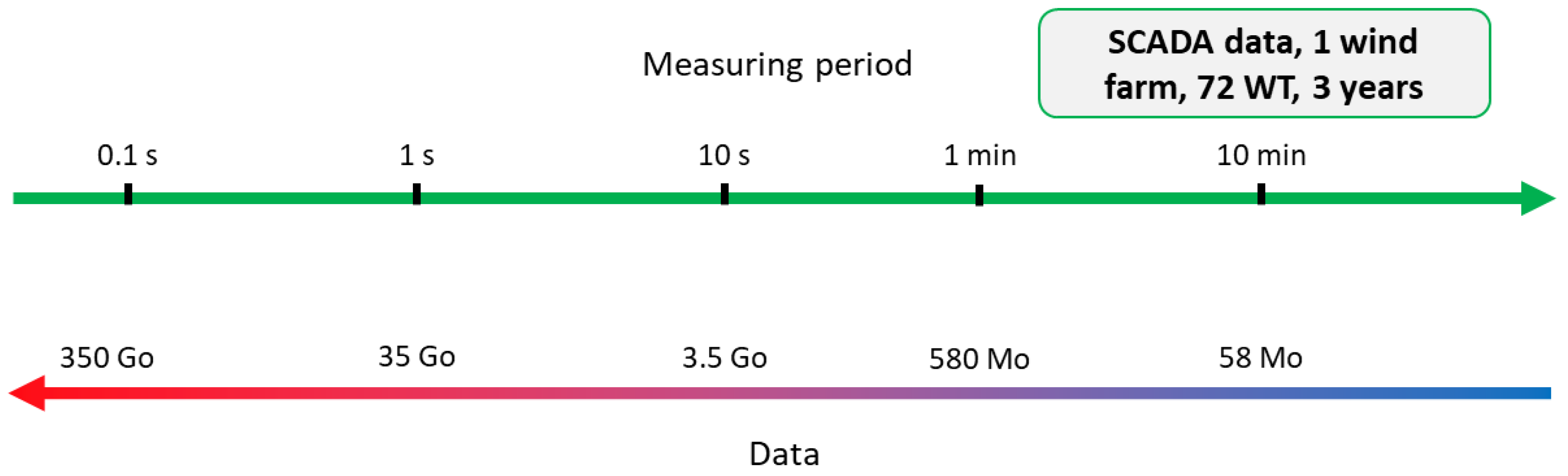
The second family of predictive maintenance relies on physical models such as that of Eder and Chen (2020) [8]. There are different physical methods enabling to estimate the WTB RUL. The most used method is based on the Miner’s rule and it is easy to operate [9,10,11,12,13,14,15,16,17,18,19,20]. Other models exist, but they are less employed due to their inherent use limits such as the method relying on the Paris–Erdogan or Walker’s elastic crack propagation law [8,21] or the stiffness degradation fatigue theories about composite materials [11]. The physical models are known to allow accurate estimations of damage behavior. However, their associated computations are extremely time consuming when considering the complete lifetime of a WT (typically 25 to 30 years). Moreover, as laid out by Jang et al. [13], a reliable WTB damage evaluation requires a 1 Hz wind speed (WS) sampling frequency because WTBs are sensitive to WS fluctuations at this frequency. As a result, because 1 Hz WS data are very hefty, and because fatigue computation via physical damage models is time consuming, the WTB damage cannot be evaluated for a large period of time [13]. Then, the industry norm is to work with 10-min aggregated signals (average, min, max, standard deviation), as recommended by the IEC standard 61400-12-1 [22]. The 10-min period has been proven to provide enough information to evaluate the energetic aspects of the WT [20]. However, as mentioned above, WTB fatigue assessment requires data with higher frequencies, which are not always archived in the SCADA systems. Figure 1 presents the differences between various aggregation intervals in terms of data volume. This situation forces to design a fatigue damage computation tool working with the 10-min SCADA data in order to be applicable to as many wind farms as possible.
The present study intends to achieve this goal to come up with a way to estimate blade damage regarding 10-min SCADA data. The presented model starts by computing the damage induced by the fluctuation of the 10-min mean WS stored in the SCADA data using the well-known Miner’s rule. This damage will be called low cycle fatigue (LCF) in this study. Then, the damage induced by WS fluctuations within each 10-min SCADA data period is investigated. To achieve this, a 1 Hz stochastic WS signal is numerically generated via a turbulence model based on the Kaimal spectrum [23,24], in correlation with the previous 10-min SCADA data. Then, the corresponding damage is again computed via the Miner’s rule. This damage will be called high cycle fatigue (HCF) in this study. Finally, by combining the LCF and the HCF, it is expected to obtain an overall relative WTB fatigue damage evaluation. Finally, applying this method to an entire wind farm enables to highlight which WT is the most damaged and allow the wind farm operator to optimize his maintenance operations. The main breakthrough here is the possibility to achieve for the first time a damage evaluation based on a physical model, considering a 1 Hz WS signal extending through the entire WT lifetime by lowering many of the computation needs.
This study is divided into four main parts. The first section deals with the data and the numeric tools at our disposal, followed by a presentation of the hypothesis of the model developed. The second section presents the LCF damage estimation methodology based on 10-min WS SCADA signals. The third section shows the HCF damage estimation methodology, based on 1 Hz simulated WS signals. The HCF damage estimation aims to be added to the LCF evaluation based on 10-min SCADA data because the fatigue is a cumulative phenomenon. Then, results are analyzed and discussed in the fourth section. Finally, the conclusion proposes a global overview of the breakthroughs brought by this study and suggests other future leads to improve the results already obtained with the present method.
2. Resources and Hypothesis
2.1. Resources
To carry out this study, we have access to 10-min aggregated signals from SCADA data (specifically, a 10-min mean WS history) of a wind farm composed of 5 MW WT from February 2017 to May 2020. Then, Matlab® programming language and FAST aeroelastic models [25] were used to estimate the aerodynamic loads leading to stress variations, and consequently, damage due to WS fluctuations. However, to estimate the inner stress in the WTB, a detailed numeric model of the WTB should be used. Because the wind turbine model installed on the studied windfarm is unknown for confidentiality issues, a 5 MW WT numeric model from the NREL library (open access) was used as reference [26,27]. This numeric model was chosen as it is the most common and most studied model in the literature. In this context, it is assumed that the evaluated fatigue damage on the numeric wind turbines will differ from the real wind turbines operating in this wind farm, but the ranking of the most damaged wind turbine is expected to remain the same. Hence, the damage computed in this project is relative and not absolute.
2.2. Considered Environmental Effects and Hypothesis
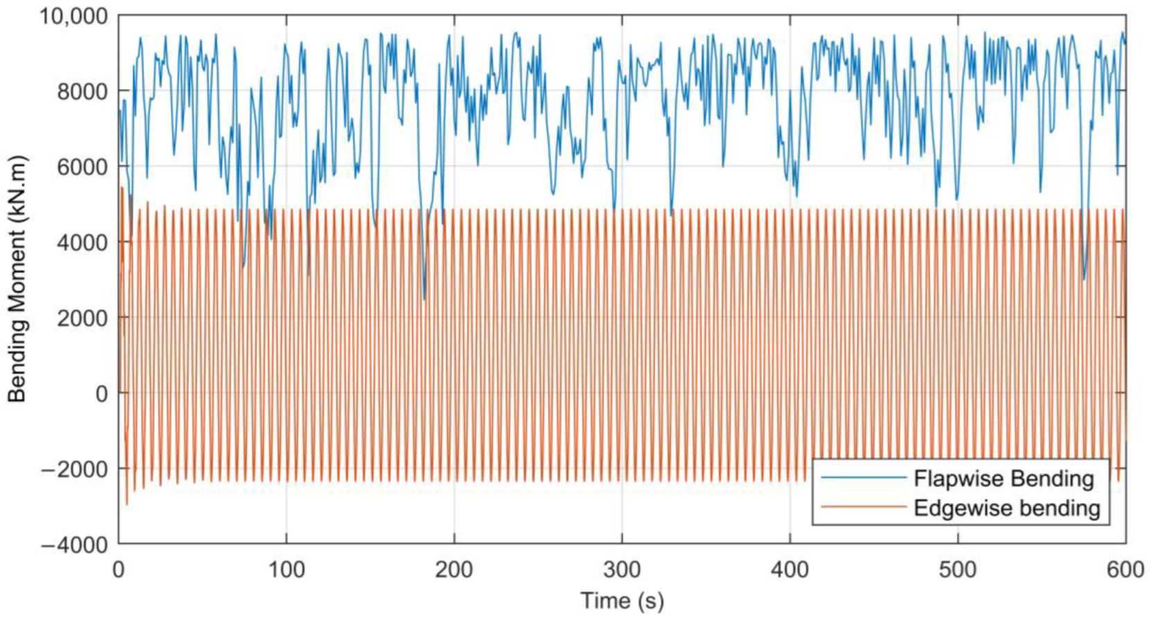
WTB fatigue is caused by different environmental factors, such as rain erosion [28], the gravity effect [29], and temperature variations, all of which can also affect the material fatigue strength [30] at different locations. The blades are submitted to two mains bending moments, the flapwise bending and the edgewise bending [20,22,31,32] (Figure 2). Because they are locations on the WTB depending almost only on flapwise bending (like the adhesive bond line in the trailing edge [8]) or on edgewise bending, it is possible to consider only one of these types of bending in such locations for fatigue purpose [8,12,22,31]. Depending on the localization on the blade root, the blade root section can be at the same time only subjected to flapwise or to edgewise bending [12,31,32]. It appears that the fatigue damage induced by flapwise bending at the blade root is much higher than the edgewise one [12,32]. Moreover, the flapwise bending is provoked by the wind while the edgewise bending is mainly caused by the weight of the blade [31,32,33]. So, the wind speed variations can be assumed to be the major factor influencing the WTB fatigue as already suggested in the scientific literature [19,32]. Thus, for simplicity, we will focus only on this aspect in the rest of this paper.
2.3. Hypothesis
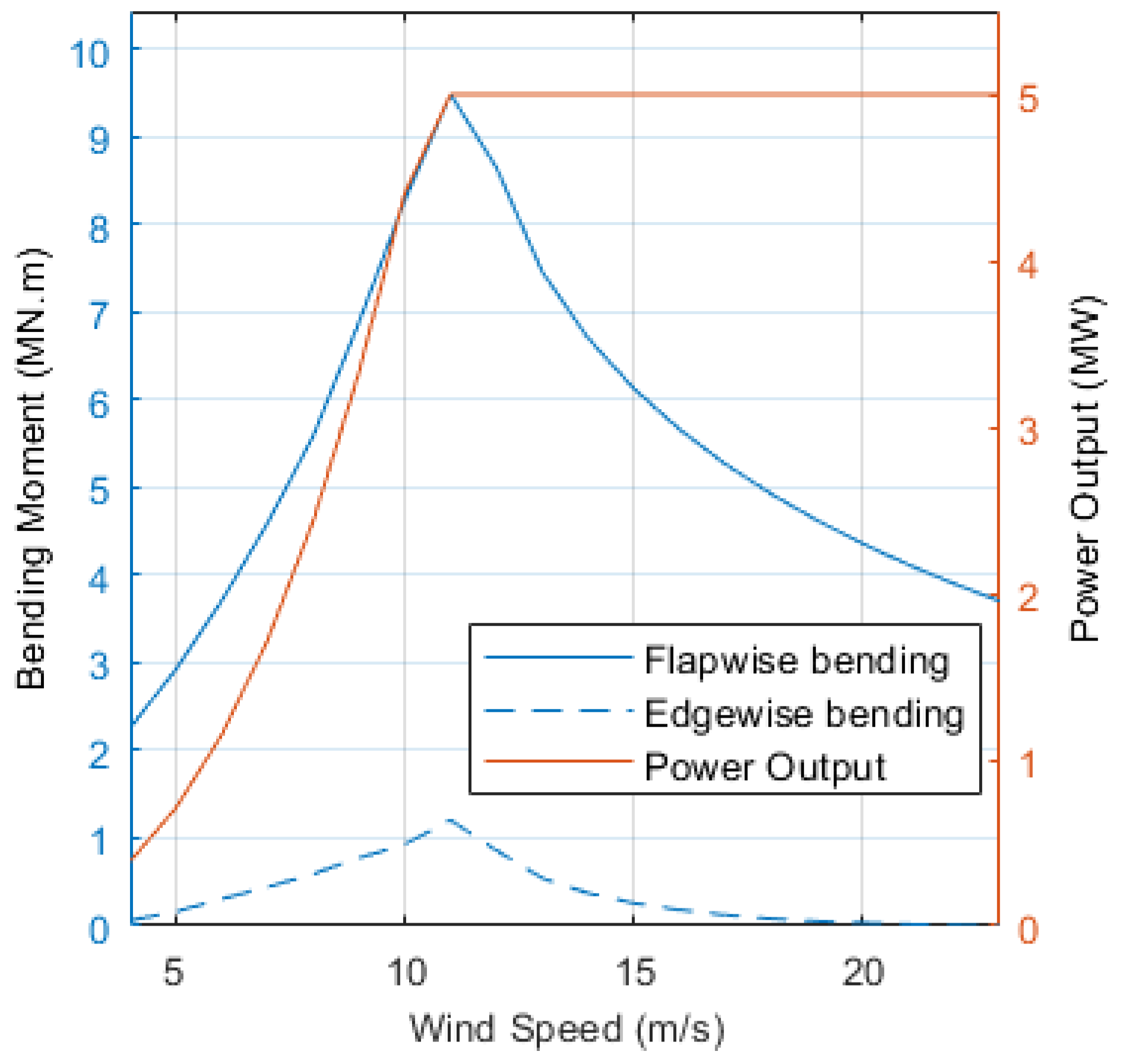
The damage is considered at the blade root section for two main reasons. Firstly, because it is expected to be the most sensitive part to fatigue issues [31,31,32,34], and secondly, because it generally has a circular section no matter the wind turbine model and the rest of the blade structural design [8,16,31,32,33], which is not publicly shared by the wind turbine OEM [33]. At the blade root, only the diameter and the skin thickness depends of the global length of the blade [26,33,35], facilitating the extrapolation of a conceivable root structure design from basic information from the numeric WTB model. The damage is due to variations in the stress within the part, which is correlated with flapwise bending and edgewise bending. Considering a zero pitch, the flapwise bending corresponds to the out-rotor plane direction while the edgewise bending is associated with the in-rotor plane direction. However, according to estimations carried out with FAST and a 5 MW wind turbine blade from the NREL library, of the two, flapwise bending would seem to be more sensitive to WS fluctuations (see Figure 3), which is why, in the present study, we focus on the stress resulting from it. Regarding the simulated 1 Hz WS signal, the simulated wind is also considered to be blowing in the rotor axis like the previous one, but it is generated stochastically using the Kaimal spectrum proposed in the FAST TurbSim module [24]. The Kaimal spectrum is often used in the wind turbine fatigue field to generate a turbulent wind field [36,37] because it has been designed for a homogeneous and flat onshore site [38]. It best describes the turbulence wind field within the atmospheric boundary layer, where the earth’s surface has a strong influence on the atmosphere [39]. This is why it is a recommended model for the wind turbine industry, according to standard IEC 61,400 [20]. Finally, because of the cumulative nature of the damage, the overall WTB damage is assumed to be the sum of the HCF and LCF damage and other factors, defined as follows:
where is the overall WTB root damage at time , is the damage due to LCF, is the damage due to HCF, is the damage induced by transient regimes (shut-down and start-up of the WT), is the damage caused by extreme environmental conditions such as storm-inducing wind velocities higher than the cut-out WS of the wind turbine (in our case, 25 m·s−1), damage due to lightening, etc., and finally, is the initial damage induced by manufacturing at time . Here, is not considered because it relies on complex mechanisms like resonance issues or sudden material failures not related to fatigue behavior, according to Chou et al. [40]. is also not considered for reasons of simplification because it relies on defects not depending on fatigue behavior and that are harsh to assess, even though they can have a strong effect on WT strength [16,41,42]. In addition, is also not considered here because it requires a finer analysis of the start-up and shut-down procedures used by the wind farm operator to assess the corresponding damage [12,43]. In the present work, only and are considered because they refer to the WTB fatigue behavior. This study introduces for the first time an estimation of the HCF based on 10-min aggregated SCADA data commonly used in the wind farm industry, enabling to evaluate the WTB fatigue damage for a long period of time covering the entire life span of the WT. Hence, the overall damage is summarized in Equation (2):
3. LCF Damage Assessment
3.1. Assessment of Stress
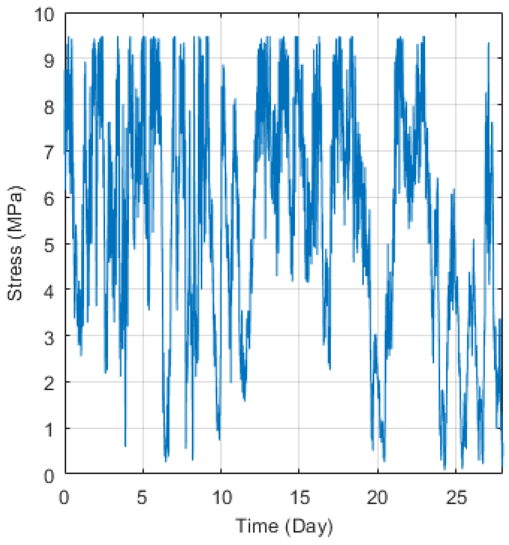
Using FAST software and the geometric properties of a 5 MW WT model from the NREL library, the flapwise bending moment () at the blade root could be estimated according to the WS (see Figure 3). Following this, and knowing the flapwise bending moment and the geometry of the WTB, it was then possible to estimate the stress history according to the mean WS history (seen at the blade root thanks to Equation (3) (see Figure 4):
with being the resulting stress [Pa]. is the maximum distance from the neutral axis, which corresponds approximately to the chord line for a WTB in bending. So, is nearly equal to half of the airfoil thickness [m] at the root [31,33]. is the moment of inertia of the WTB root section [m4]. To obtain , the skin thickness of the blade at the root section [m] must be known. However, this information is not provided with the numerical WTB model used in this study. Furthermore, the WTB root thickness for a 5 MW WT varies strongly (from 50 to 80 mm) depending on the sources [44,45,46], making it difficult to obtain a reliable extrapolation. So, it has been arbitrarily chosen to approximate via the following empirical law [33]:
where [m] is the rotor radius (here, m for the 5 MW FAST WT model).
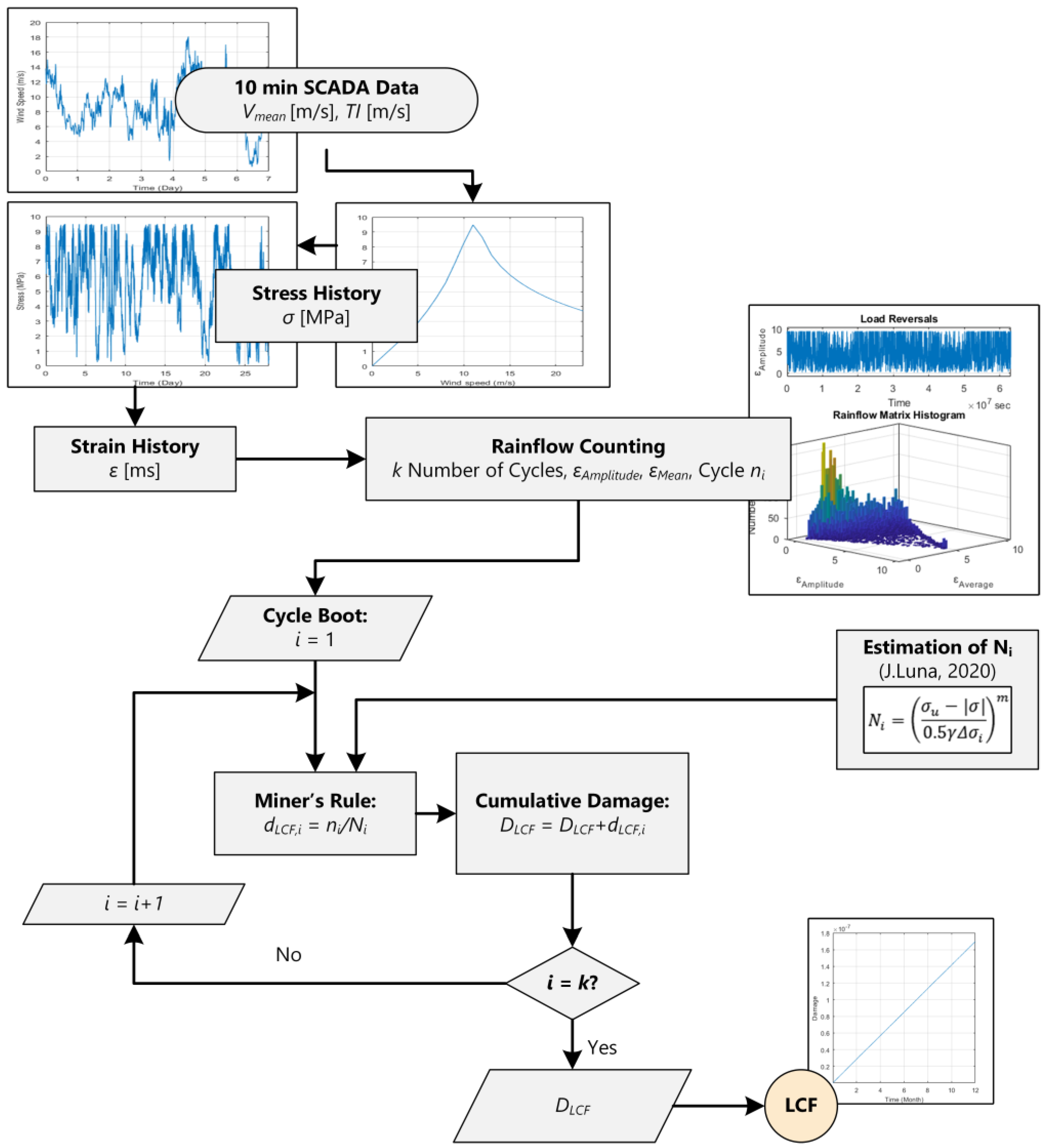
The next step is to carry out the Rainflow Counting algorithm (RFC) as defined in [47] according to the standards [14,20], to have the stress cycle characterization regarding the stress history.
Here, [MPa] is the stress range amplitude of the cycles, corresponds to the number of cycles according to the cycle amplitude , refers to the -th stress cycle. Then, the WTB damage can be estimated as presented in the next section.
3.2. Damage Evaluation Based on 10-min SCADA Data
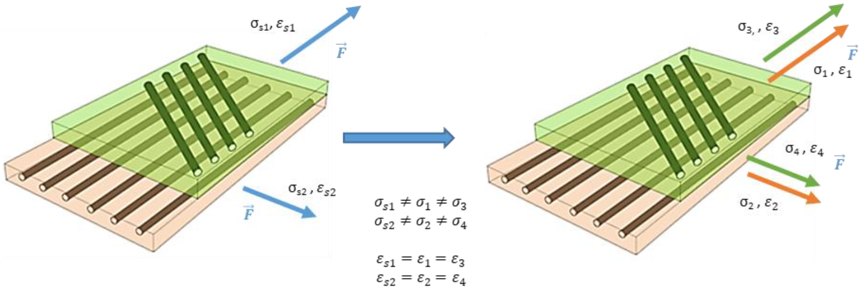
Many studies rely on stress variation to carry out WTB damage evaluation [9,10,11,13]. However, according to [14], it is recommended to work with the strain variation rather than stress variation in order to evaluate the damage level in composite materials due to the fatigue phenomenon. One reason for this is that the strain remains the same between the plies composing the laminate when a force is applied to the latter, while it is not the case with the stress (see Figure 5).
The guide proposed by Germanischer Lloyd, or DNV GL, since 2013 [14] lays out an approach based on the strain and the Goodman diagram of the considered laminate to assess the damage behavior due to fatigue. For a certain i-th strain cycle characteristic, the corresponding can be known via Equation (6), with the parameters explained in the nomenclature:
According to [14], it is expected that
Here, and can be derived from the previous RFC of the stress. Knowing the stacking of layers within the blade root section, the corresponding Young’s modulus of the material at the WTB root can be obtained [48]. After which, once the Young’s modulus is evaluated, the RFC of the stress can be converted into the RFC of the strain via the Hooke’s law, providing and for each strain cycle. Then, starting from Equation (5), the RFC of the strain allows to estimate the following:
where is the maximum strain to rupture of the weakest ply composing the laminate.
Finally, as recommended by the standards [14,20], via the Miner’s rule (Equation (9)) with provided by Equation (6) and given by the RFC of the strain, an estimation of the WTB’s LCF damage for the corresponding -th cycle can be computed:
Then, the global LCF damage is computed as the sum of encountered within the period of study. The global methodology is summarized in Figure 6:
4. HCF Damage Evaluation
According to [13], it is necessary to work with an approximately 1 Hz WS signal to ensure a reliable damage estimation. WS signal histories with high sampling rates are uncommon, and where available, their processing is heavily computing resource-intensive because of the sheer volume of data involved (600 times more than 10-min SCADA data, as shown in Figure 1). To overcome these issues, the approach presented herein consists in estimating the damage due to a 1 Hz WS signal for a 10-min period parametrized with a mean WS and turbulence intensity () defined as follows [13,49]:
Here, is the standard deviation of the measured WS over a 10-min period and [m·s−1] is the measured mean WS within this period.
TurbSim FAST’s module is used here to generate the required WS signals [24]. Series of WS signals are generated for all the wind characteristics (in terms on mean WS and ) that the WT can meet in normal operating conditions as defined by the norm IEC-61400-1 [20]. So, each series of WS signals is simulated regarding a specific mean WS and from a range of values starting from the cut-in WS to the cut-out WS and a of 1% to 50% as advised by [20]. The model runs with the Kaimal spectrum to generate a turbulent wind flow as recommended by the standards [14,20]. The Kaimal spectrum is used in the wind turbine industry to generate stochastic and turbulent wind flow [50].
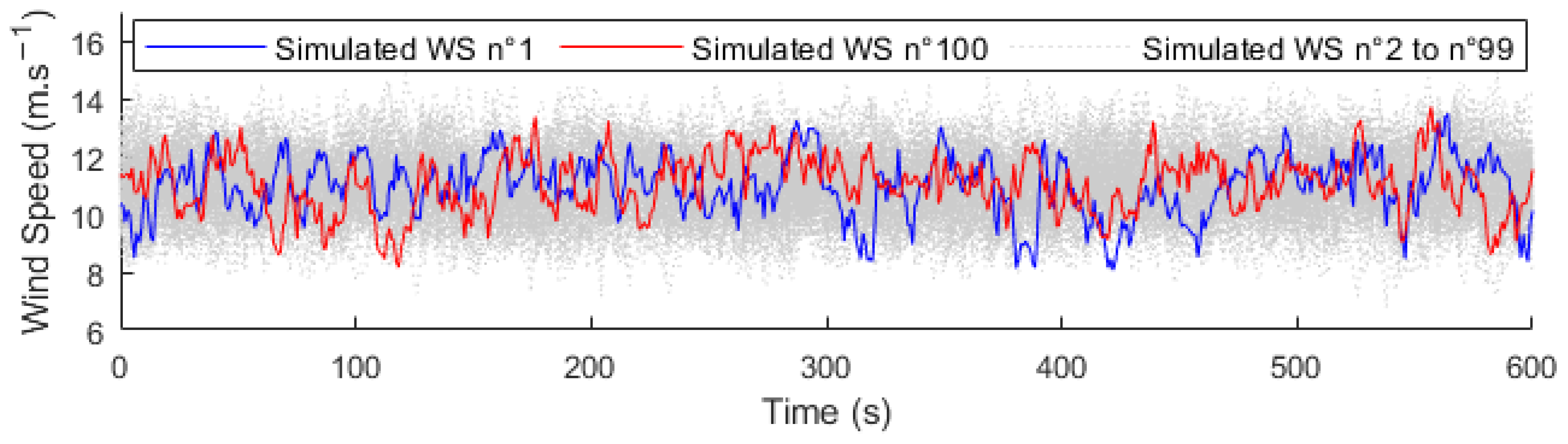
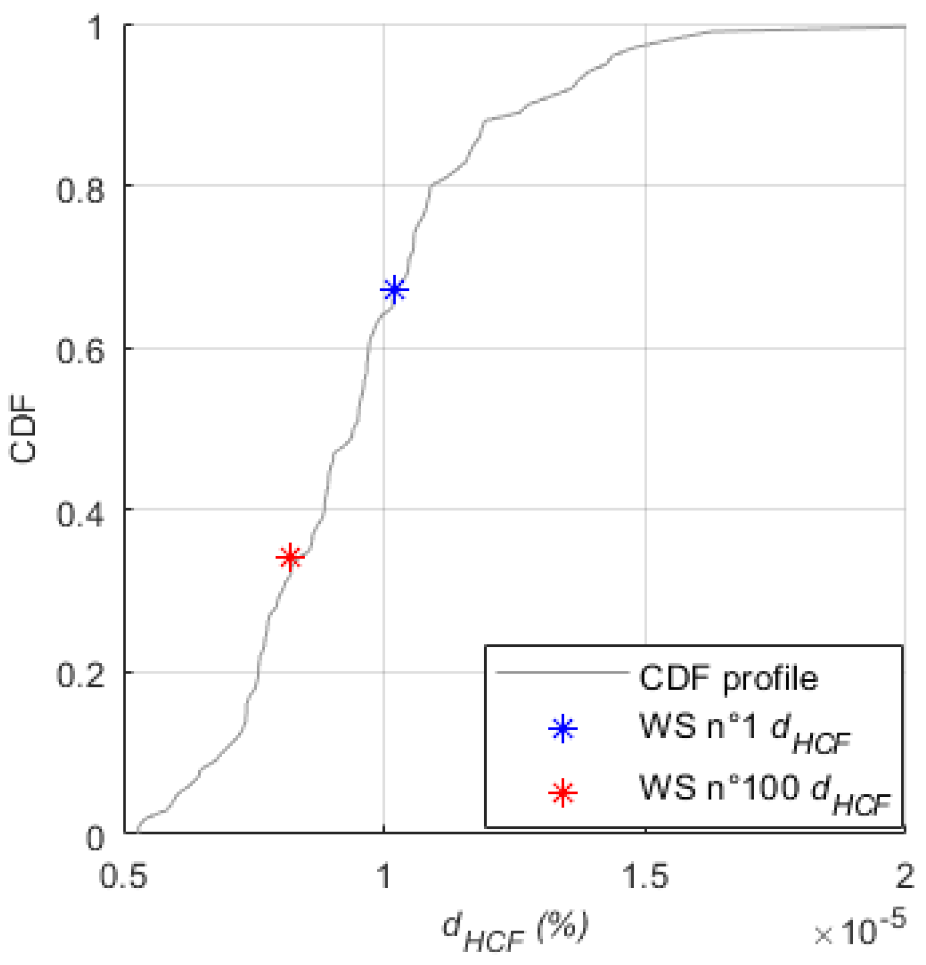
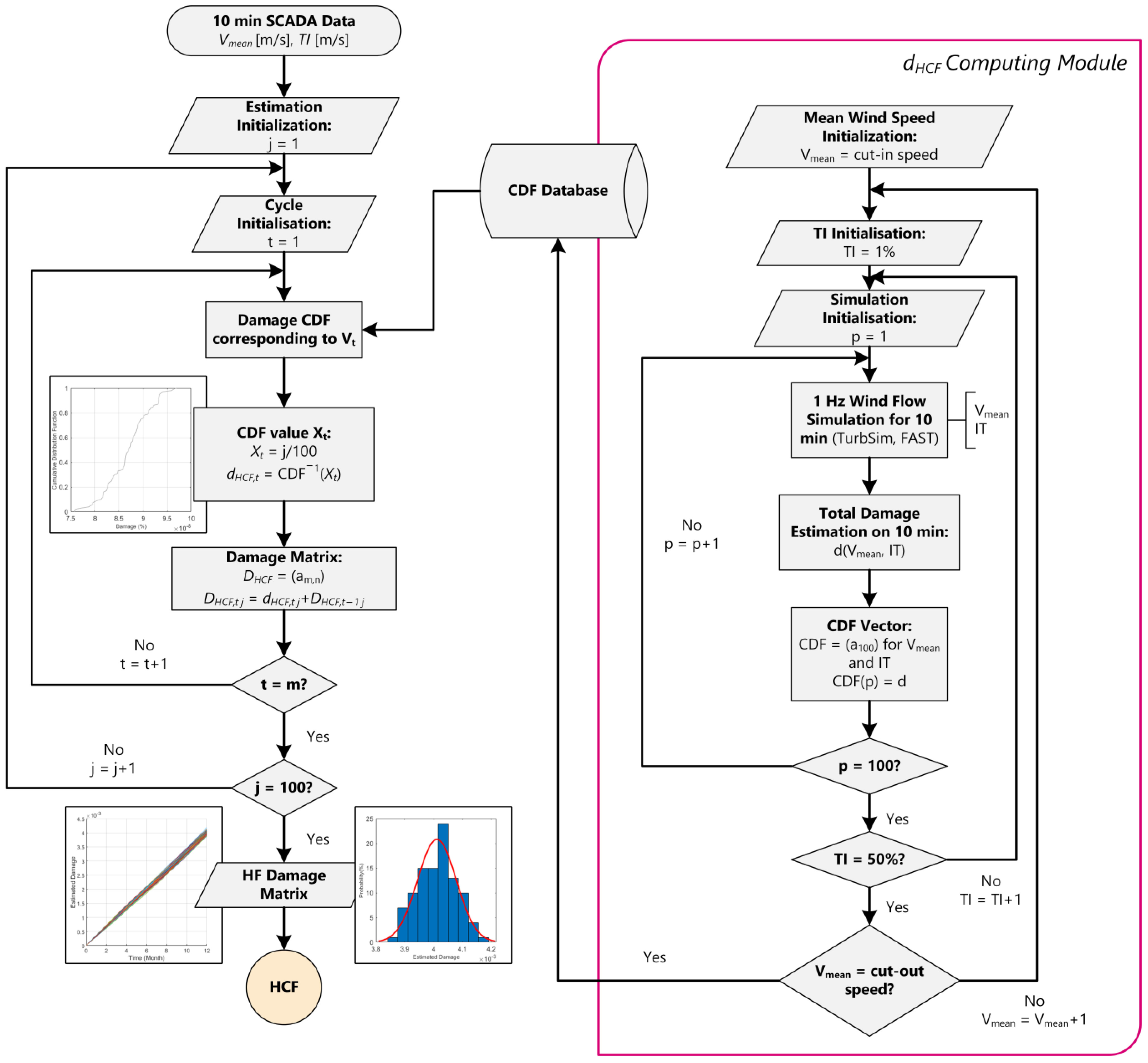
Because the WS signals are generated stochastically trying to reflect the wind’s behavior in the nature [51], a generated WS signal can differ from another even if they share the same and . So, it is expected that the resulting WTB damage from a generated WS signal can also differ from another WS signal, even if those signals have the same parameters— and . That is why a series composed of numerous stochastic simulations must be carried out for each and , to cover a wide variety of possible signals—and thus, of resulting damage. Each WS signal is simulated at a 1 Hz frequency for a 10-min period with the and parameters associated to the WS series that they belong to, as shown in Figure 7. After 100 simulations, the damage distribution tends to maintain a single shape, converging to the same distribution values. Hence, it has been chosen to fix at 100 the number of WS signals within each WS series. Then, for each simulation (or WS signal), the equivalent HCF damage is assessed using the methodology presented in Section 3.2. Because each simulation corresponds to a proper , the results can be expressed under the form of a cumulative distribution function (CDF) of for each WS series and parameter (see Figure 8).
Then, for each 10-min period of the SCADA data history, the associated and the are identified and the WS series damage CDF with the corresponding parameters is selected. Next, the equivalent for this 10-min period is chosen according to the cumulative distribution value (CDV) .
where of the selected CDF is chosen according to the damage percentile considered, with the time steps and being the functions describing the damage CDF. Finally, by cumulating the selected for the entire 10-min mean WS history, the overall WTB damage can be calculated:
Hence, can be computed for a long period (1 year in this case) and the probability distribution function (PDF) of can be extrapolated by varying the value of . The assessment methodology used is summarized in Figure 9.
5. Results and Discussion
5.1. Damage Estimation
Regarding Equation (2), the global WTB damage can be computed as the sum of and . To evaluate the WTB damage for several years, it has been chosen to concatenate the 1-year WS history by the number of years required to have an approximation of the entire life WS history. However, from the results obtained, it appears that is much higher than (see Table 1). These results can be explained by the fact that the sampling frequency of the signal used for the fatigue estimation strongly influences the WTB damage estimation, as described by [52]. According to these results, could be approximated as equal to to simplify the presented WTB damage estimation process. Thus, the following relation can be assumed, in the case where only the operation running regime is considered:
Based on the hypothesis presented in Section 2.3, leading to Equation (2), it was decided to consider only the WTB damage due to the operation running regime and a relatively simple geometry at the blade root. In Section 5.3, a discussion about how to increase the reliability of the results is presented.
5.2. Impact of TI and on HCF Damage
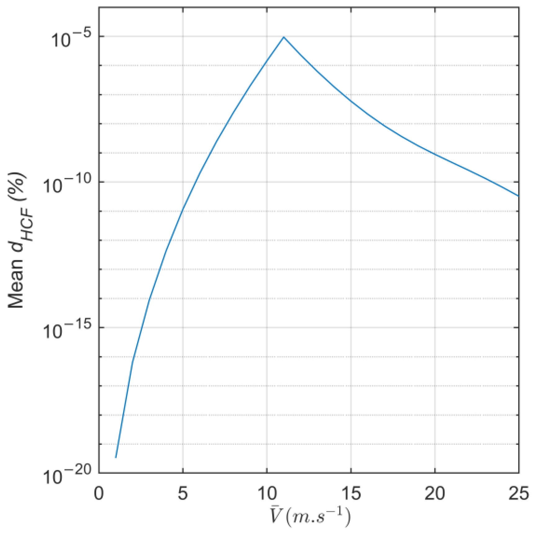
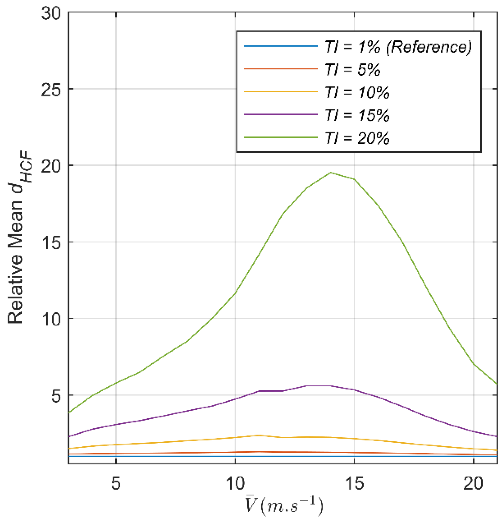
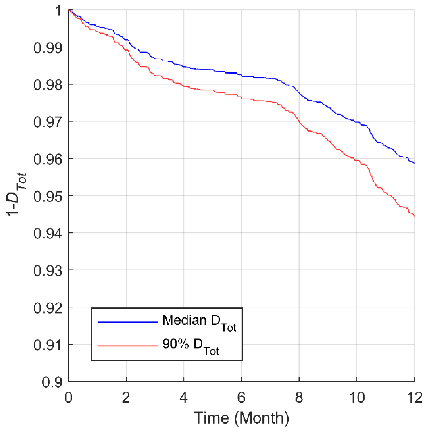
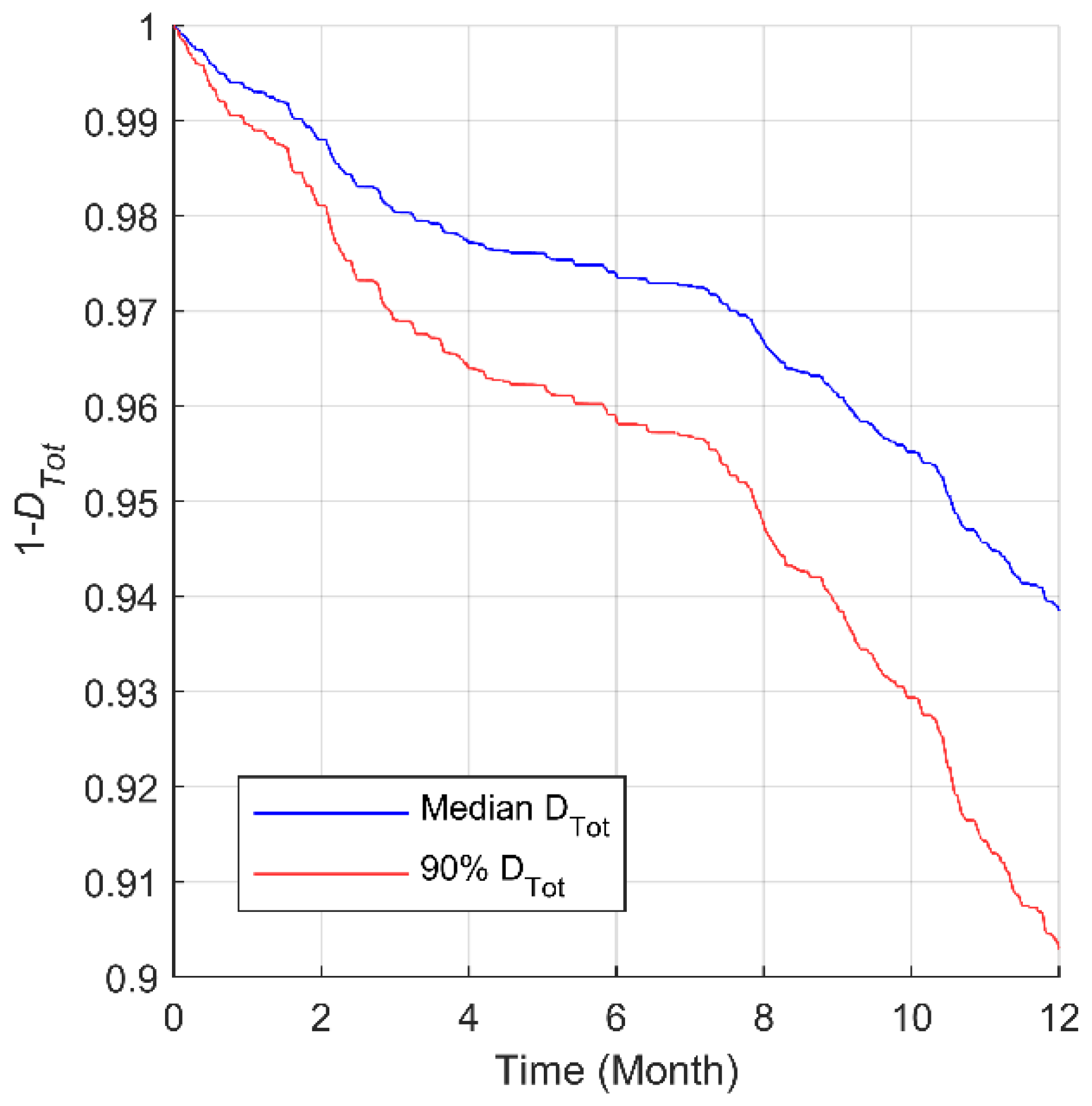
According to the results presented in Figure 10, it appears that has a strong impact on . The computed reaches its maximum at WS 11 m·s−1, corresponding to the moment where the WT nominal power and maximum bending moment are met. However, such wide differences can call into question the need to consider any other WS than 11 m·s−1. The is another parameter influencing , albeit to a lesser extent. Based on the results of Figure 11, for a WS 11 m·s−1, is increased by 30%, with going from 1% to 5%, and by 1320%, with a going from 1% to 20%. This result is explained by the fact that with a growing , the amplitude of the bending cycles, and thus of the strain cycles, increases, leading to an increase in . Concerning the evaluation of , a increase from 10% to 12% represents a damage increase of 50% with going from 0.04% to 0.06%, as shown in Figure 12 and Figure 13, after 1 year.
5.3. Study Case
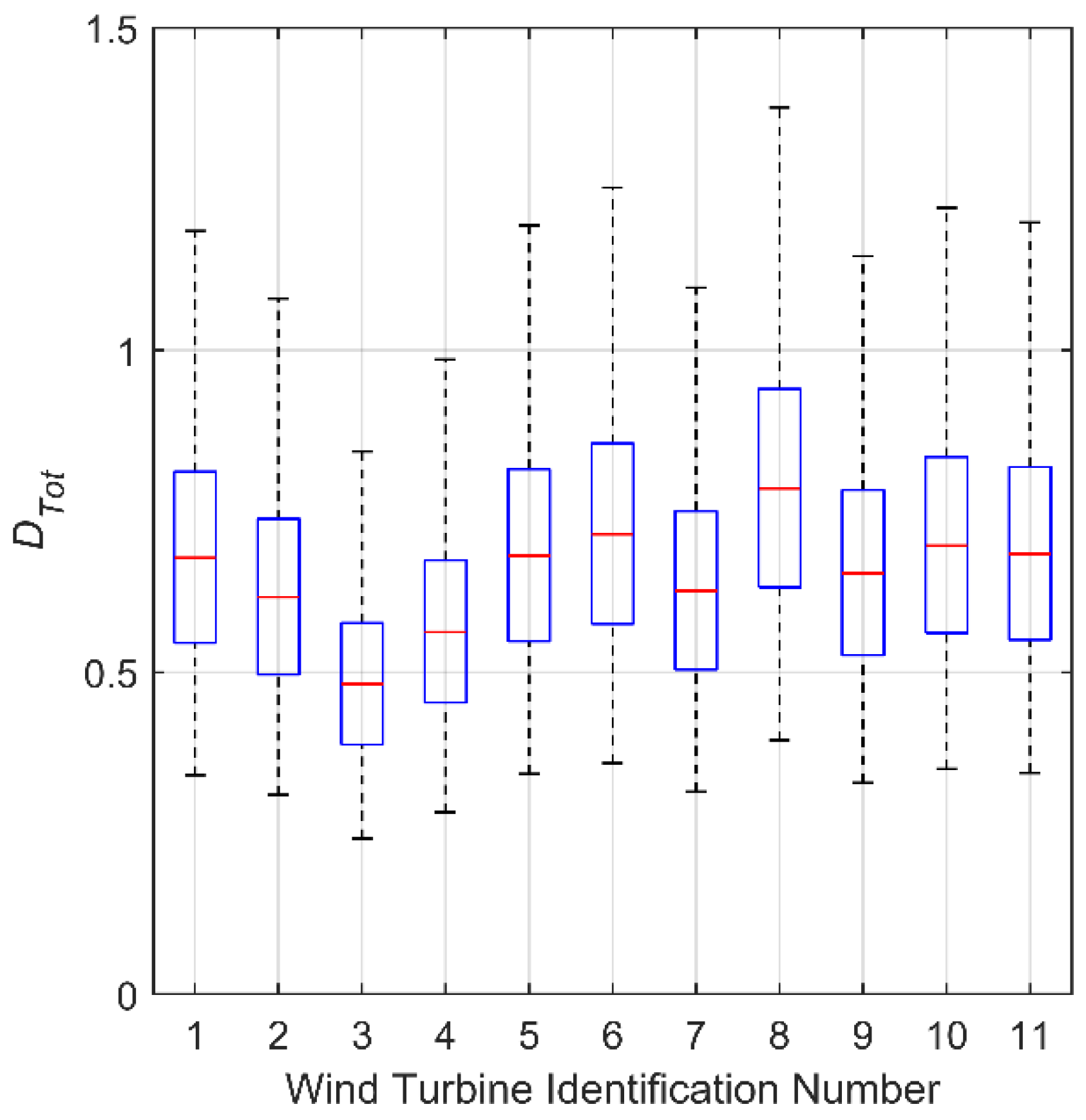
This damage model needs to be calibrated despite the good results presented here, for several reasons. Firstly, the thickness of the blade root section was estimated via Equation (4), but uncertainties about the real blade root section thickness persist. Secondly, the layer stack of the material of the blade root section can differ between WTB models [28]. However, this damage model can already be used as a tool to rank WT within the same park according to the evaluated fatigue damage considering the 10-min mean WS SCADA data. In our study case, was computed for 11 WT of the same wind farm for a 20-year period (see Figure 14). This result can lead to the wind farm operator adopting its O&M schedule and budget accordingly by focusing on WT n°8 (which is assessed as the most damaged WT) in this example.
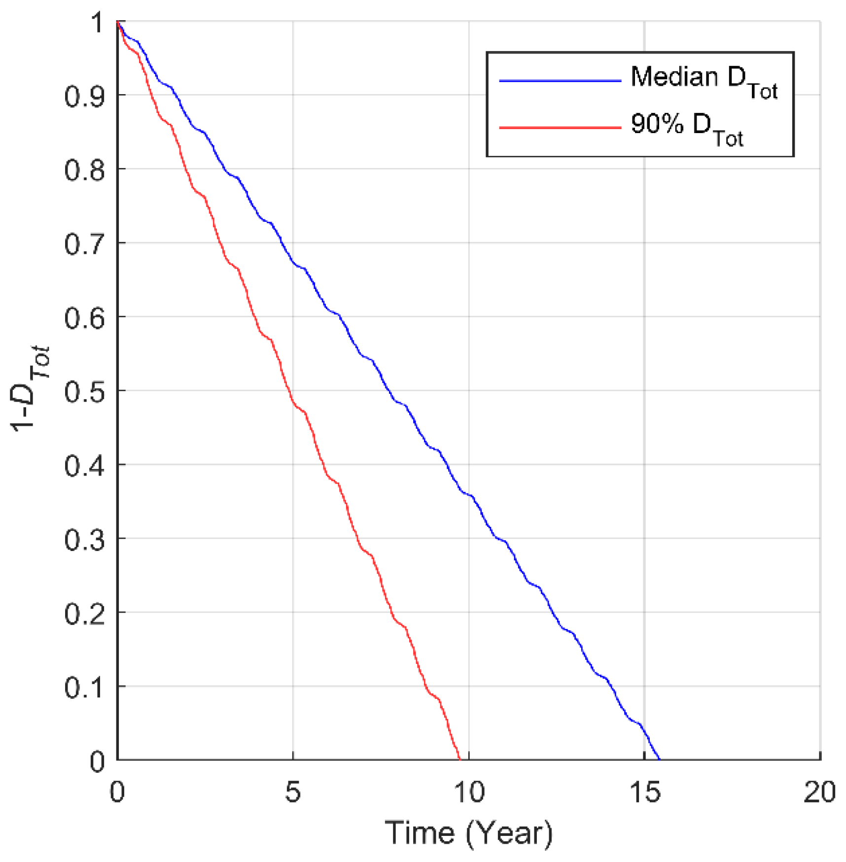
Then, once this model is calibrated, more specific results could be extracted. As an example, taking WT n°8 mentioned above, the profiles could be computed (see Figure 15). Take note that the oscillation of is due the season impact, the distribution of the wind flow parameters changing depending on the season.
The damage presented here is only relative. To have an absolute damage evaluating tool, in addition to the calibration of the damage model, other factors influencing the damage behavior must be considered, notably the impact of the running regime on the WTB damage. In the literature, it appears that the current damage models only focus on a specific running regime [7,8,9,10,11,12,13,15,29,43,53,54]. However, according to them, each running regime does matter in the WTB damage evaluation field. So, as a next step, to improve the damage calculation, the future damage model must take into account other operating regimes influencing as expressed in Equation (1). This means that the impact of the transient regimes on must be investigated to obtain a more reliable computation of . Then, because this tool is developed to help the windfarm operator taking O&M decisions, the next damage model should consider the impact of these operations on the WTB damage level as explained by [6]. Ultimately, because WTs are operated for a long period (around 20 years), it would be interesting to investigate the impact of the climate change on the WTB damage. As explained by [55], climate change can have an important effect on WT performance, and so, on their fatigue damage.
6. Conclusions
In this paper, a method allowing to evaluate WTB high cycle fatigue damage considering 10-min SCADA data is proposed. Firstly, a WTB damage assessment based on 10-min SCADA data and considering the equivalent damage due to a 1 Hz fluctuating WS signals, based on rainflow counting and Palmgren–Miner’s rule was put in place. The LCF damage and the HCF damage were separated. The equivalent WTB damages for a 10-min period with a 1 Hz stochastic wind under different environmental parameters were assessed and stored in the form of a damage CDF database. Then, by cumulating the estimated WTB damage CDF for each 10-min SCADA data period, the HCF damage for a long period of time could be computed for the first time. Next, the CDV was selected in terms of the damage percentile of interest to the operator. These different steps enable to have a PDF of the calculated HCF damage, thus providing wind farm operators a more complete decision-making tool regarding their maintenance strategy. After comparing the HCF damage with the LCF damage, the LCF damage appeared to be negligible as compared to that for the HCF, leading to the assumption that the global WTB damage is effectively equal to the latter when only operation running conditions are considered.
Secondly, the WTB damage assessed while taking only operation running conditions into account must also consider other factors, such as transient regimes and extreme environmental conditions, because these can influence the damage behavior of the WTB. Moreover, the model must be calibrated because assumptions will have been made regarding the blade root thickness or the material properties, which could lead to uncertainties about the computed effective damage. The next step will therefore consist in carrying out computations while considering the transient regimes and extreme environmental conditions of WTs and to calibrate the damage model to ensure a more reliable estimation of WTB fatigue damage.
Author Contributions
Conceptualization, A.C. and A.T.; Software, A.C., P.C. and A.O.-F.; Validation, A.T. and P.C.; Investigation, A.C.; Resources, A.T. and P.C.; Data curation, P.C.; Writing—original draft, A.C.; Writing—review & editing, A.C., A.T. and P.C.; Supervision, A.T. and P.C. All authors have read and agreed to the published version of the manuscript.
Funding
This research was funded by CRSNG, grant number #RDCPJ 543389-19.
Data Availability Statement
A publicly available wind turbine model and was used in this study. This model can be found here: https://www.nrel.gov/wind/nwtc/fastv8.html. The wind speed data used in this study is available on request from the corresponding author. The data are not publicly available due to confidentiality clause.
Conflicts of Interest
The authors declare no conflict of interest.
Nomenclature
| Characteristic short-term structural member resistance for tension | |
| Characteristic short-term structural member resistance for compression | |
| Partial safety factor for material | |
| Partial safety factor for material | |
| Mean value of characteristic cycles | |
| Amplitude of characteristic cycles | |
| Slope parameter of S/N curve | |
| Vacuum infusion molding effect | |
| Post-cure polymerization effect | |
| Temperature effect | |
| Non-woven unidirectional fibers effect | |
| Post-cure polymerization effect | |
| Local safety factor at the trailing edge | |
| Ageing effect | |
| Temperature effect |
References
- DNV GL Energy Transition Outlook DNV GL’s Energy Transition Outlook 2020. Available online: https://eto.dnvgl.com/2020/index.html (accessed on 4 December 2020).
- Zhu, C.; Li, Y.; Zhu, C.; Li, Y. Reliability Analysis of Wind Turbines; IntechOpen: London, UK, 2018; ISBN 978-1-78984-148-0. [Google Scholar]
- Li, H.; Peng, W.; Huang, C.-G.; Guedes Soares, C. Failure Rate Assessment for Onshore and Floating Offshore Wind Turbines. J. Mar. Sci. Eng. 2022, 10, 1965. [Google Scholar] [CrossRef]
- Mishnaevsky, L. Repair of wind turbine blades: Review of methods and related computational mechanics problems. Renew. Energy 2019, 140, 828–839. [Google Scholar] [CrossRef]
- IEA. Technology Roadmap: Wind Energy, 2013rd ed.; IEA: Paris, French, 2013. [Google Scholar]
- Nielsen, J.S.; Sørensen, J.D. Bayesian Estimation of Remaining Useful Life for Wind Turbine Blades. Energies 2017, 10, 664. [Google Scholar] [CrossRef] [Green Version]
- Asgarpour, M.; Sørensen, J.D. Bayesian based Prognostic Model for Predictive Maintenance of Offshore Wind Farms. Int. J. Progn. Health Manag. 2018, 9, 2696. [Google Scholar] [CrossRef]
- Eder, M.A.; Chen, X. FASTIGUE: A computationally efficient approach for simulating discrete fatigue crack growth in large-scale structures. Eng. Fract. Mech. 2020, 233, 107075. [Google Scholar] [CrossRef]
- Liu, P.F.; Chen, H.Y.; Wu, T.; Liu, J.W.; Leng, J.X.; Wang, C.Z.; Jiao, L. Fatigue Life Evaluation of Offshore Composite Wind Turbine Blades at Zhoushan Islands of China Using Wind Site Data. Appl. Compos. Mater. 2023, 30. [Google Scholar] [CrossRef]
- Yisu, C.; Di, W.; Haifeng, L.; Wei, G. Quantifying the Fatigue Life of Wind Turbines in Cyclone-Prone Regions | Elsevier Enhanced Reader. Available online: https://reader.elsevier.com/reader/sd/pii/S0307904X22002682?token=AFBC21C659B18F1E6EFDFD5A21555CD6748B1151BE736E6E2C7BDCB79A9893EC29A491306D7632A6B1F674BD3D38877A&originRegion=us-east-1&originCreation=20220620161427 (accessed on 20 June 2022).
- Sanchez, H.; Sankararaman, S.; Escobet, T.; Puig, V.; Frost, S.; Goebel, K. Analysis of two modeling approaches for fatigue estimation and remaining useful life predictions of wind turbine blades. Proc. Eur. Conf. PHM Soc. 2016, 11, 1640. [Google Scholar]
- Jiang, Z.; Moan, T.; Gao, Z. A Comparative Study of Shutdown Procedures on the Dynamic Responses of Wind Turbines. J. Offshore Mech. Arct. Eng. 2015, 137, 011904. [Google Scholar] [CrossRef]
- Jang, Y.J.; Choi, C.W.; Lee, J.H.; Kang, K.W. Development of fatigue life prediction method and effect of 10-min mean wind speed distribution on fatigue life of small wind turbine composite blade. Renew. Energy 2015, 79, 187–198. [Google Scholar] [CrossRef]
- Germanischer, L. Guideline for the Certification of Wind Turbine; Germanischer Lloyd: Hamburg, Germany, 2010. [Google Scholar]
- Bergami, L.; Gaunaa, M. Analysis of aeroelastic loads and their contributions to fatigue damage. J. Phys. Conf. Ser. 2014, 555, 012007. [Google Scholar] [CrossRef] [Green Version]
- Marín, J.C.; Barroso, A.; París, F.; Cañas, J. Study of fatigue damage in wind turbine blades. Eng. Fail. Anal. 2009, 16, 656–668. [Google Scholar] [CrossRef]
- Vera-Tudela, L.; Kühn, M. Analysing wind turbine fatigue load prediction: The impact of wind farm flow conditions. Renew. Energy 2017, 107, 352–360. [Google Scholar] [CrossRef]
- Tibaldi, C.; Henriksen, L.C.; Hansen, M.H.; Bak, C. Wind turbine fatigue damage evaluation based on a linear model and a spectral method: Wind turbine fatigue damage evaluation. Wind Energy 2016, 19, 1289–1306. [Google Scholar] [CrossRef]
- Ragan, P.; Manuel, L. Comparing Estimates of Wind Turbine Fatigue Loads Using Time-Domain and Spectral Methods. Wind Eng. 2007, 31, 83–99. [Google Scholar] [CrossRef]
- IEC 61400-1; Wind Turbines Part 1: Design Requirements, International Electrotechnical Commission. IEC: Geneva, Switzerland, 2019.
- Valeti, B.; Pakzad, S.N. Estimation of Remaining Useful Life of a Fatigue Damaged Wind Turbine Blade with Particle Filters. In Dynamics of Civil Structures, Volume 2; Pakzad, S., Ed.; Springer International Publishing: Cham, Switzerland, 2019; pp. 319–328. ISBN 978-3-319-74420-9. [Google Scholar]
- IEC 61400-12-1 Ed. 2.0 b:2017; Wind Energy Generation Systems–Part 12-1: Power Performance Measurements of Electricity Producing Wind Turbines. International Electrotechnical Commission: Geneva, Switzerland, 2017.
- Kaimal, J.C.; Wyngaard, J.C.; Izumi, Y.; Coté, O.R. Spectral characteristics of surface-layer turbulence. Q. J. R. Meteorol. Soc. 1972, 98, 563–589. [Google Scholar] [CrossRef]
- Jonkman, B.J.; Buhl, M.L. TurbSim User’s Guide; National Renewable Energy Laboratory: Oak Ridge, TN, USA, 2006. [Google Scholar]
- Jonkman, J.M.; Buhl, M.L., Jr. FAST User’s Guide—Updated August 2005; National Renewable Energy Laboratory: Oak Ridge, TN, USA, 2005. [Google Scholar]
- Dykes, K.L.; Rinker, J. WindPACT Reference Wind Turbines; National Renewable Energy Laboratory: Oak Ridge, TN, USA, 2018. [Google Scholar]
- Jonkman, J.; Butterfield, S.; Musial, W.; Scott, G. Definition of a 5-MW Reference Wind Turbine for Offshore System Development; National Renewable Energy Laboratory: Oak Ridge, TN, USA, 2009. [Google Scholar]
- Hu, W.; Chen, W.; Wang, X.; Jiang, Z.; Wang, Y.; Verma, A.S.; Teuwen, J.J.E. A computational framework for coating fatigue analysis of wind turbine blades due to rain erosion. Renew. Energy 2021, 170, 236–250. [Google Scholar] [CrossRef]
- Barnes, R.H.; Morozov, E.V.; Shankar, K. Improved methodology for design of low wind speed specific wind turbine blades. Compos. Struct. 2015, 119, 677–684. [Google Scholar] [CrossRef]
- Hawileh, R.A.; Abu-Obeidah, A.; Abdalla, J.A.; Al-Tamimi, A. Temperature effect on the mechanical properties of carbon, glass and carbon–glass FRP laminates. Constr. Build. Mater. 2015, 75, 342–348. [Google Scholar] [CrossRef]
- Lars, D.; Torben, J.L.; Jaocb, W.; John, D.S.; Rune, K.; Johnny, P.; Mads, L.; Vasileios, K. Wind Turbine Blades Handbook; Bladena: Taastrup, Denmark, 2017. [Google Scholar]
- Manwell, J.F.; McGowan, J.G.; Rogers, A.L. Wind Energy Explained; John Wiley & Sons: Hoboken, NJ, USA, 2009; ISBN 978-4-470-01500-1. [Google Scholar]
- Joncas, S. Thermoplastic Composite Wind Turbine Blades. Ph.D. Thesis, Delft University of Technology, Delft, The Netherlands, 2010. [Google Scholar]
- Zárate-Miñano, R.; Anghel, M.; Milano, F. Continuous wind speed models based on stochastic differential equations. Appl. Energy 2013, 104, 42–49. [Google Scholar] [CrossRef]
- Bortolotti, P.; Tarres, H.C.; Dykes, K.; Merz, K.; Sethuraman, L.; Verelst, D.; Zahle, F. Systems Engineering in Wind Energy–WP2.1 Reference Wind Turbines; National Renewable Energy Laboratory: Oak Ridge, TN, USA, 2019. [Google Scholar]
- Yi, W.; Lu, Z.; Hao, J.; Zhang, X.; Chen, Y.; Huang, Z. A Spectrum Correction Method Based on Optimizing Turbulence Intensity. Appl. Sci. 2021, 12, 66. [Google Scholar] [CrossRef]
- Hong, X.; Li, J. Stochastic Fourier spectrum model and probabilistic information analysis for wind speed process. J. Wind Eng. Ind. Aerodyn. 2018, 174, 424–436. [Google Scholar] [CrossRef]
- Cheynet, E.; Jakobsen, J.B.; Obhrai, C. Spectral characteristics of surface-layer turbulence in the North Sea. Energy Procedia 2017, 137, 414–427. [Google Scholar] [CrossRef]
- Couche limite atmosphérique–Centre National de Recherches Météorologiques. Available online: https://www.umr-cnrm.fr/spip.php?rubrique186 (accessed on 6 March 2023).
- Chou, J.-S.; Chiu, C.-K.; Huang, I.-K.; Chi, K.-N. Failure analysis of wind turbine blade under critical wind loads. Eng. Fail. Anal. 2013, 27, 99–118. [Google Scholar] [CrossRef]
- Li, J.; Wang, J.; Zhang, L.; Huang, X.; Yu, Y. Study on the Effect of Different Delamination Defects on Buckling Behavior of Spar Cap in Wind Turbine Blade. Adv. Mater. Sci. Eng. 2020, 2020, 6979636. [Google Scholar] [CrossRef]
- Murdy, P.; Hughes, S.; Barnes, D. Characterization and repair of core gap manufacturing defects for wind turbine blades. J. Sandw. Struct. Mater. 2022, 24, 2083–2100. [Google Scholar] [CrossRef]
- Jiang, Z.; Xing, Y. Load mitigation method for wind turbines during emergency shutdowns. Renew. Energy 2022, 185, 978–995. [Google Scholar] [CrossRef]
- Sun, Z.; Sessarego, M.; Chen, J.; Shen, W.Z. Design of the OffWindChina 5 MW Wind Turbine Rotor. Energies 2017, 10, 777. [Google Scholar] [CrossRef] [Green Version]
- Hiebel, M.; Schlipf, D. Case Study: D50 Offshore Wind Turbine. Aerodyn Eng. 2018. [Google Scholar]
- We are LM Wind Power—The Leading Rotor Blade Supplier to the Wind Industry | LM Wind Power. Available online: https://www.lmwindpower.com/ (accessed on 8 March 2023).
- Rainflow Counts for Fatigue Analysis–MATLAB Rainflow. Available online: https://www.mathworks.com/help/signal/ref/rainflow.html?searchHighlight=C#d123e146736 (accessed on 13 April 2022).
- Kollar, L.P.; Springer, G.S. Mechanics of Composite Structures; Cambridge University Press: Cambridge UK; New York, NY, USA, 2003; ISBN 978-0-521-80165-2. [Google Scholar]
- Kim, D.-Y.; Kim, Y.-H.; Kim, B.-S. Changes in wind turbine power characteristics and annual energy production due to atmospheric stability, turbulence intensity, and wind shear. Energy 2021, 214, 119051. [Google Scholar] [CrossRef]
- Dong, L.; Lio, W.H.; Simley, E. On turbulence models and lidar measurements for wind turbine control. Wind Energy Sci. 2021, 6, 1491–1500. [Google Scholar] [CrossRef]
- Farouk, C. Etude du Comportement Stochastique et Cyclique du vent en ALGÉRIE; Presses Académiques Francophones: Paris, French, 2019; ISBN 978-3-8416-2904-3. [Google Scholar]
- Chrétien, A.; Tahan, A.; Cambron, P.; de Oliveira-Filho, A.M. Impact of 10 Min Average Wind Speed SCADA Data on the Wind Turbine Blade Damage Prediction Compared to 1 Second Signal. In Proceedings of the 1st International Electronic Conference on Processes: Processes System Innovation, Online, 17–31 May 2022. [Google Scholar]
- Requate, N.; Meyer, T.; Hofmann, R. From wind conditions to operational strategy: Optimal planning of wind turbine damage progression over its lifetime; Dynamics and control/Wind turbine control. WES 2022. [Google Scholar] [CrossRef]
- Salimi-Majd, D.; Azimzadeh, V.; Mohammadi, B. Loading Analysis of Composite Wind Turbine Blade for Fatigue Life Prediction of Adhesively Bonded Root Joint. Appl. Compos. Mater. 2015, 22, 269–287. [Google Scholar] [CrossRef]
- Bisoi, S.; Haldar, S. Impact of climate change on dynamic behavior of offshore wind turbine. Mar. Georesour. Geotechnol. 2017, 35, 905–920. [Google Scholar] [CrossRef]
Figure 1.
Schema showing the relation between data weight and the measuring period for a wind farm composed of 72 WT for a period of 3 years.
Figure 1.
Schema showing the relation between data weight and the measuring period for a wind farm composed of 72 WT for a period of 3 years.

Figure 2.
Flapwise and edgewise bending moments for a mean wind speed of 11 m·s−1 and a TI = 20%.

Figure 3.
Mean bending moments and output power as a function of the wind speed.

Figure 4.
Estimated stress history for a period of 4 weeks for a single 5 MW wind turbine.

Figure 5.
Schema showing the relationship between plies strains within a laminate.

Figure 6.
Flowchart showing the process leading to the estimation of the LCF damage from SCADA data.
Figure 6.
Flowchart showing the process leading to the estimation of the LCF damage from SCADA data.

Figure 7.
Simulation of 100 stochastic wind speed signals with and TI = 10% for a period of 10 min.

Figure 8.
Estimated damage CDF for a WS series with the following parameters: and TI = 10% over a period of 10 min.
Figure 8.
Estimated damage CDF for a WS series with the following parameters: and TI = 10% over a period of 10 min.

Figure 9.
Flowchart showing the process leading to the estimation of the HCF damage from the SCADA data.
Figure 9.
Flowchart showing the process leading to the estimation of the HCF damage from the SCADA data.

Figure 10.
Mean WTB damage dHCF regarding a generated 1 Hz wind speed signal for a 10-min period as function of the with a fixed TI = 10%.
Figure 10.
Mean WTB damage dHCF regarding a generated 1 Hz wind speed signal for a 10-min period as function of the with a fixed TI = 10%.

Figure 11.
Relative mean WTB damage dHCF regarding a generated 1 Hz wind speed signal for a 10-min period as a function of the for different TI, taking the mean dHCF for TI = 1% as reference.
Figure 11.
Relative mean WTB damage dHCF regarding a generated 1 Hz wind speed signal for a 10-min period as a function of the for different TI, taking the mean dHCF for TI = 1% as reference.

Figure 12.
Graphic of 1 − DTot for 1 WT imposing TI = 10% for a 1-year period. In blue, the median DTot, computed with the 50th percentile of DHCF. In red, 90% DTot, computed with the 90th percentile of DHCF.
Figure 12.
Graphic of 1 − DTot for 1 WT imposing TI = 10% for a 1-year period. In blue, the median DTot, computed with the 50th percentile of DHCF. In red, 90% DTot, computed with the 90th percentile of DHCF.

Figure 13.
Graphic of 1 − DTot for 1 WT imposing TI = 12% for a 1-year period. In blue, the median DTot, computed with the 50th percentile of DHCF. In red, 90% DTot, computed with the 90th percentile of DHCF.
Figure 13.
Graphic of 1 − DTot for 1 WT imposing TI = 12% for a 1-year period. In blue, the median DTot, computed with the 50th percentile of DHCF. In red, 90% DTot, computed with the 90th percentile of DHCF.

Figure 14.
Boxplot of WTB damage DTot for 11 WT within a same park after a 10-year period.

Figure 15.
Graphic of 1 − DTot for WT n°8. In blue, the median DTot, computed with the 50th percentile of DHCF. In red, 90% DTot, computed with the 90th percentile of DHCF.
Figure 15.
Graphic of 1 − DTot for WT n°8. In blue, the median DTot, computed with the 50th percentile of DHCF. In red, 90% DTot, computed with the 90th percentile of DHCF.


Table 1.
Table showing the difference between LCF and HCF (TI = 1%) damage estimations for different lengths of the study period.
Table 1.
Table showing the difference between LCF and HCF (TI = 1%) damage estimations for different lengths of the study period.
| Period of Study | DLCF (t) | Mean DHCF (t) | DHCF (t)/DLCF (t) |
|---|---|---|---|
| 1 year | 7.94 × 10⁻⁵ | 4.02 | 5.06 × 10⁴ |
| 20 years | 1.56 × 10⁻³ | 7.12 × 101 | 4.56 × 10⁴ |
Disclaimer/Publisher’s Note: The statements, opinions and data contained in all publications are solely those of the individual author(s) and contributor(s) and not of MDPI and/or the editor(s). MDPI and/or the editor(s) disclaim responsibility for any injury to people or property resulting from any ideas, methods, instructions or products referred to in the content. |
© 2023 by the authors. Licensee MDPI, Basel, Switzerland. This article is an open access article distributed under the terms and conditions of the Creative Commons Attribution (CC BY) license (https://creativecommons.org/licenses/by/4.0/).
Share and Cite
MDPI and ACS Style
Chrétien, A.; Tahan, A.; Cambron, P.; Oliveira-Filho, A. Operational Wind Turbine Blade Damage Evaluation Based on 10-min SCADA and 1 Hz Data. Energies 2023, 16, 3156. https://doi.org/10.3390/en16073156
AMA Style
Chrétien A, Tahan A, Cambron P, Oliveira-Filho A. Operational Wind Turbine Blade Damage Evaluation Based on 10-min SCADA and 1 Hz Data. Energies. 2023; 16(7):3156. https://doi.org/10.3390/en16073156
Chicago/Turabian StyleChrétien, Antoine, Antoine Tahan, Philippe Cambron, and Adaiton Oliveira-Filho. 2023. "Operational Wind Turbine Blade Damage Evaluation Based on 10-min SCADA and 1 Hz Data" Energies 16, no. 7: 3156. https://doi.org/10.3390/en16073156
Note that from the first issue of 2016, this journal uses article numbers instead of page numbers. See further details here.