Design and Implementation of a Particulate Matter Measurement System for Energy-Efficient Searching of Air Pollution Sources Using a Multirotor Robot

Abstract

Analyzing air pollutants is of key importance for the environmental protection goals. High concentrations of particulate matter (PM) have a particularly negative impact on human life and health. The use of an autonomous multirotor flying robot (drone) for the purposes of locating PM sources requires the design of a dedicated measurement system from scratch. The aim of this study was to make the most important design decision, which is the correct localization of the inlet of the measurement system, taking into account disturbances in the flow field caused by the rotors. To achieve this, a computational model was built with the use of a finite-volume method in Ansys Fluent software. Based on its results, a novel criterion was proposed and applied. In addition to the trivial position outside the rotors on the extended arm, it gave the second location in the space limited by the rotors below the robot. Finally, a robot prototype was built, and a series of verification experiments were carried out, first indoors and then outdoors, at different levels of ambient PM concentrations with and without a pollution source. The field results were compiled as histograms and scatter plots and clearly demonstrated the validity of the adopted criterion. The determination coefficient between measured concentrations showed a stronger relationship when the rotors were operating. Furthermore, in cases with a present pollution source, higher concentrations were observed around the internal sensor, making it more suitable for the studied application.

1. Introduction

Air pollution analysis, especially particulate matter (PM) monitoring, is of crucial importance for environmental protection objectives. Polluted air is currently one of the most important environmental threats to human health and well-being. According to a study [1], it is the fourth leading factor in increasing the risk of death. Factors, such as smoking, high blood pressure, dietary risks, and high blood glucose levels, also contribute to the risk. The literature shows a significant relationship between public health and air pollution [2]. For example, the high concentration of ${\mathrm{PM}}_{2.5}$ particles is responsible for respiratory diseases. The study [3] indicates that there is an increased risk of AECOPD (acute exacerbation of chronic obstructive pulmonary disease) under conditions of high concentrations of solid particles, low ambient temperature, and low humidity. These conditions occur especially in the winter season when, due to low emissions, increased concentrations are observed. The literature [4] also indicates that high concentrations of PM reduce the benefits of outdoor activities, such as walking or cycling.

The use of flying robots for particle measurement has been reported in the literature, for example, in [5,6]. In [7], a balloon/drone-based platform was developed to monitor ${\mathrm{PM}}_{2.5}$ pollutants at different altitudes. The [8] study compares the results of PM and ozone measurements using a fixed-wing drone and an aircraft carrier at high altitudes in a low troposphere. Similar research using drones with wings is presented in [9]. The work [10] uses a multirotor robot to measure air pollution during fires in a large area (that is, more than 1000 ha). Similar studies on the measurement of bioaerosols, which are aerosols of biological origin, are presented in [11,12]. The work [13] evaluated the suitability of drones for volcanic observations, where a method was proposed to measure the wind, PM, and gas velocities under field conditions. The work [14] presents the possibility of using a drone to automatically neutralize CO and PM pollutants with the use of activated carbon absorbing sheets. In [15], a robot-based four-rotor system was presented for high-resolution measurement of the vertical distribution of PM particle concentration, black carbon, ozone, nitrogen oxides (${\mathrm{NO}}_{\mathrm{x}}$), and carbon monoxide. Similar approaches are presented in [16,17,18]. The article [19] estimated a 3D spatial profile of air pollution spread at intersections in densely populated areas. The methodology of cooperation between stationary measurements, measurements using drones, and the atmospheric dispersion modeling process (WRF-CFD model) was applied. The comparability of the data obtained experimentally and those obtained through the modeling process was indicated to guarantee the possibility of identifying hotspots, which are areas with significantly higher concentrations. However, the modeling process assumed that there were no other sources of pollution other than traffic. Similar studies are described in [20], where vertical profiles of solid particles were determined in a street canyon, which is a street surrounded by tall buildings. In [21], a system was designed to measure air pollution, consisting of a low-cost Arduino-compatible measuring system and a multirotor hexacopter robot. However, the system is now equipped with sensors to measure only CO, ${\mathrm{NO}}_2$, temperature, and humidity. The presented system was used to measure these pollutants under urban conditions, and then, based on the collected data, pollution maps were generated. A similar low-cost system that can be equipped with up to nine different sensors is shown in [22]. With the proposed solution, many harmful chemicals, such as ammonia, hexane, benzene, carbon monoxide, and carbon dioxide, as well as combustible substances, such as hydrogen and methane, can be detected. Furthermore, a very important function is the ability to perform particulate matter measurements: ${\mathrm{PM}}_{2.5}$ and ${\mathrm{PM}}_{10}$. The work [23] aimed to develop a unified long-range communication and sensor system as an innovative platform for atmospheric measurements using a multi-rotor robot.

A detailed analysis of the effectiveness of PM measurements using drones is presented in [24]. It was shown that the influence of robot rotors on the measurement process has little effect on the particle size distribution but strongly influences the particle concentration. In the example of ${\mathrm{PM}}_{2.5}$ particles, differences in measured concentration ranging from −70% to more than 400% were demonstrated when comparing the measurements before and after turning on the rotors. It was also indicated that both the sensor mounting method and the location of the inlet of the measurement system are critical aspects of the measurements performed with the use of drones. There has also been guidance that the area directly above the drone appears to be the optimal place to mount the sensor. In [25], particulate matter air pollution tests were carried out for ${\mathrm{PM}}_{1.0}$, ${\mathrm{PM}}_{2.5}$, and ${\mathrm{PM}}_{10}$ using inexpensive sensors mounted on an unmanned aerial vehicle. The analysis included the change in the measured concentration values depending on the flight altitude of the drone. The decision tree method was used, which allowed one to determine the optimal flight height of the measurement drone in a specific area.

Flying robots present significant challenges in terms of the dimensions and weight of the measuring system that can be mounted on them, making it generally impossible to install laboratory-grade measurement instruments on them. Consequently, miniaturized and low-cost sensors [26,27] are commonly employed in this type of robot for monitoring air pollution. The selection of sensors for a measurement system must consider not only connection interface, power requirements, dimensions, and weight, but also the method of particulate matter measurement [28], such as gravimetric, optical, and microbalance. The study [29] presents an innovative sensor calibration algorithm, while also discussing the impact of atmospheric conditions, such as humidity, temperature, and ambient light intensity on measurement results, particularly the negative effects of high humidity on measurement accuracy. The article [26] provides an overview of 50 low-cost PM sensors from a developer’s perspective. Several studies [30,31] have been conducted to evaluate the performance of low-cost sensors under different environmental conditions. The most extensive research on this topic, presented in [32], analyzes the measurement properties of 40 different low-cost sensors and compares their data to that of laboratory-grade instruments. Using the insights gained from these studies, the appropriate sensor type can be selected for the robot being developed.

In summary, a dedicated multirotor flying robot can be employed to not only measure but also autonomously locate sources of air pollution [33]. However, the operation of robot rotors causes significant disruptions to the natural airflow and gas-transported particle fields, which can negatively impact measurements. One of the greatest research gaps in this area is the inability of a robot to automatically locate the source of pollutants in an energy-efficient manner. This is a complex issue that requires not only the incorporation of appropriate search algorithms [34], but also the determination of the appropriate sensor location and the structure of the measurement system. The current literature contains conflicting design guidelines that primarily focus on measurement accuracy but may not be suitable for source-location applications. For example, overestimating the measured concentrations may be beneficial in practical applications, as the pollution plume becomes weaker as it moves away from the source. The measured concentrations are then only slightly higher than the ambient concentration level. Therefore, the objective of the study is to estimate the disturbance of the natural flow field caused by the rotors of a dedicated flying robot. Estimation will allow for the correct design of the measurement system. Another goal is to trace the trajectory online and then to obtain guidance to reach the source. The preliminary findings of our research [35], which include both computational fluid dynamics (CFD) simulations and an experimental flight test of a measurement system with an estimated inlet location, have confirmed the proposed methodology. To further enhance the approach, a computer model of the flow field will be developed to optimize the location of the measurement system inlet based on new design criteria. Real field measurements on a large scale will then be performed, and correlation analyzes will be performed for PM sensors, taking the inlet location into account. The results obtained from this study will allow improvements in the design of the autonomous robot measurement system, as well as improvements in the control system for a more accurate and efficient source location of pollution. It is important to note that the proper design of the measurement system increases the energy efficiency of the robot. A more sensitive measurement system leads to faster detection, identification, and neutralization of pollution. Furthermore, the initial search can be carried out on a sparser grid of points, resulting in a shorter flight time required for the drone [36], ultimately leading to a reduction in energy consumption.

2. Model-Based Measurement System Design

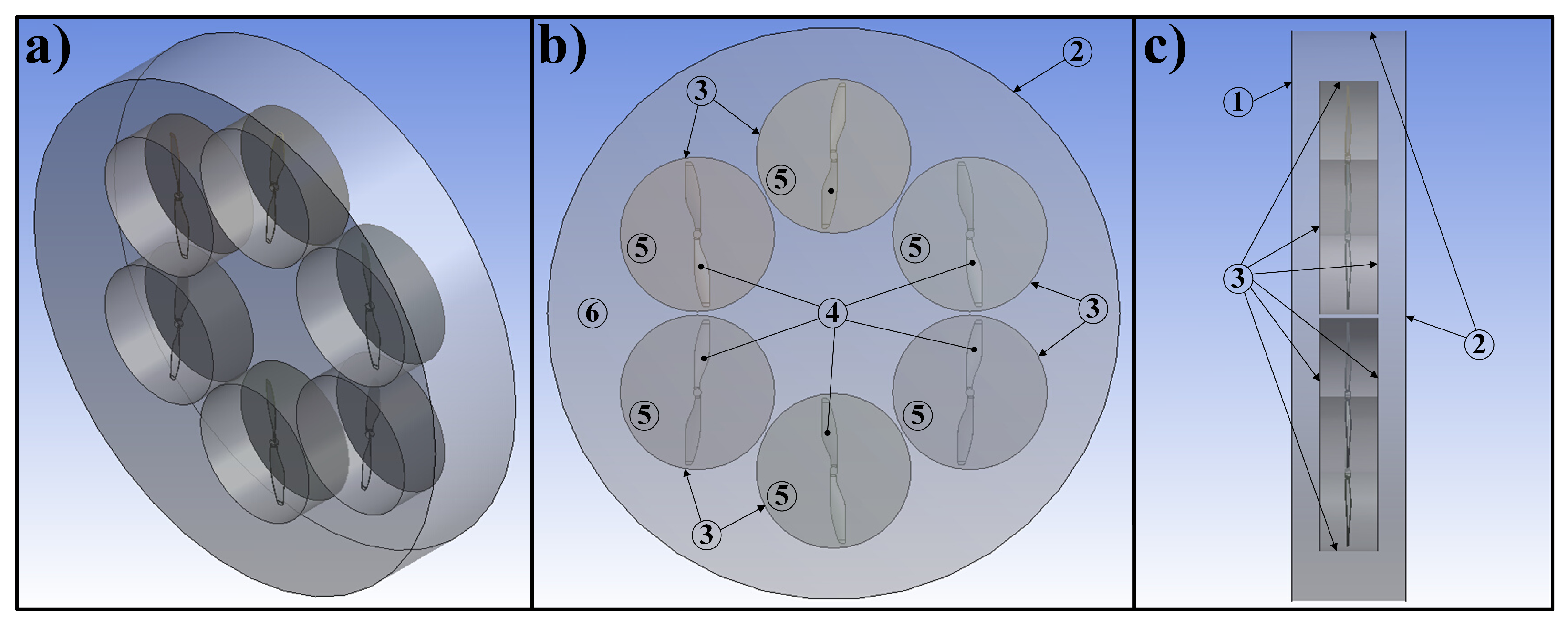
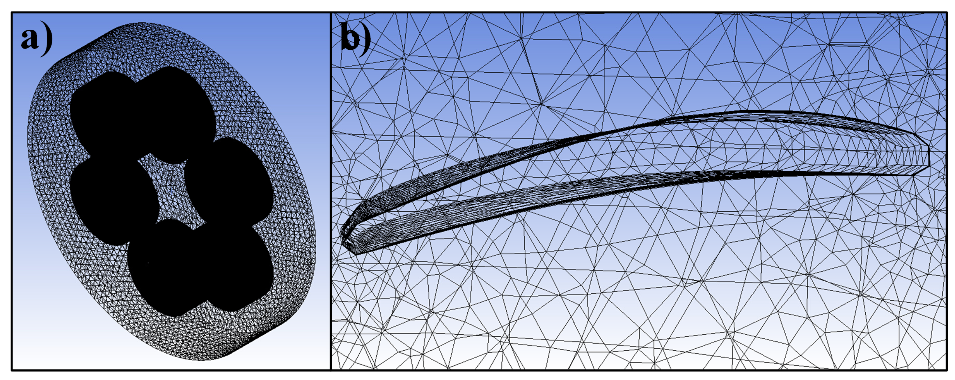
2.1. CFD Model

The present study uses a computational fluid dynamics (CFD) model to analyze a flying hexacopter robot, which has a six-rotor configuration shown in Figure 1a. This research builds on previous work [35,37] which described the methodology for the development of the computational model, presented the comparison of the results for various rotor configurations, and identified the optimal one. The mesh independence of the solution was also examined and obtained, with the criterion adopted that the difference from the previous step should be less than 10% for the next step in computational mesh refinement. For example, in the case of a configuration with one rotor, the difference in the rotor parameters was about 1%, and in the case of velocity magnitude, about 8%. The validity of the model was established by comparing it with experimental data obtained from a custom-built single-propeller dynamometer station. Factors such as thrust force, torque, and mechanical power were compared, with the most significant difference found for mechanical power, which was approximately 10%. When comparing the configuration of six rotors with a single rotor configuration, the differences amounted to approximately 5%. These results were considered accurate, and the modeling process was deemed correct. It is important to note that the model used in this analysis is a simplification of the actual system, as it includes only the rotors and excludes the body and supporting structure of the robot. The fundamental aspect of drone design is to ensure that these volumes do not significantly impact the air flow generated by the rotors. Therefore, the proper truss-shaped geometry of the arms minimizes their influence on the flow field. As previously reported in [37], the flow streamlines do not intersect the region where the body of the drone would be located, indicating that the primary flow bypasses it.

The model was developed using the finite-volume method (FVM) implemented in Ansys Fluent software. It is based on the Navier–Stokes equations, which are derived from the principles of mass conservation and momentum [38]. Simplifications were made by assuming a lack of mass sources, external and gravitational forces, and a constant fluid density. This gives a mass conservation equation in a control volume as

$$\nabla ·\mathit{u}=0$$

(1)

Since momentum in a control volume remains constant, the conservation of momentum implies that momentum can only change through the action of forces based on Newton’s laws. The corresponding equation in terms of the volume of the particle is expressed as

$$\rho \left[\frac{\partial \mathit{u}}{\partial t}+\left(\mathit{u}·\nabla \right)\mathit{u}\right]=-\nabla p+\nabla ·\left(\overline{\overline{\tau }}\right)$$

(2)

where $\rho$ is the density of the fluid, $\mathit{u}$ is the velocity vector in the Cartesian coordinate system, and p is the static pressure. According to the general deformation law of the Newtonian viscous fluid given by Stokes, the stress tensor $\overline{\overline{\tau }}$ is expressed as

$$\overline{\overline{\tau }}=\mu \left[\left(\nabla \mathit{u}+\nabla {\mathit{u}}^T\right)-\frac{2}{3}\nabla ·\mathit{u}\mathit{I}\right]$$

(3)

where $\mu$ is the kinetic viscosity, and $\mathit{I}$ is the identity tensor. The approximate solution is calculated using the $RANS$ (Reynolds-average Navier–Stokes) model, which decomposes the solution variables in instantaneous (accurate) equations into means and variable components. For the flow velocity $u_i$ in direction $x_i$ ($i=1,2,3$) and the scalar quantities $\varphi$, this can be written as

$$u_i\left(x_i,t\right)={\overline{U}}_i\left(x_i\right)+u_i^{\prime }\left(x_i,t\right),\varphi \left(x_i,t\right)=\overline{\mathsf{\Phi }}\left(x_i\right)+{\varphi }^{\prime }\left(x_i,t\right)$$

(4)

where ${\overline{U}}_i$ and $u_i^{\prime }$ are the average and time-varying components of velocity, respectively, and $\overline{\mathsf{\Phi }}$ and ${\varphi }^{\prime }$ are the average and time-varying components of scalar quantities such as pressure, energy, or intensity. The averaging process in the time period T can be described as follows

$${\overline{U}}_i\left(x_i\right)=\underset{T\to \infty }{lim}{\int }_0^T{u}_i\left(x_i,t\right)dt,\overline{\mathsf{\Phi }}\left(x_i\right)=\underset{T\to \infty }{lim}{\int }_0^T\varphi \left(x_i,t\right)dt$$

(5)

The standard model of $k-\omega$ proposed by Wilcox [39] is based on the transport equations of the kinetic energy of the turbulence k and the specific dissipation rate $\omega$. The shear stress transport (SST) $k-\omega$ model [40,41] includes a mixing function designed to activate the standard $k-\omega$ model when it has a value of one and to activate the transformed model $k-ϵ$ when zero. This model also features the principal turbulent shear stress transport when defining turbulent viscosity. These characteristics make the SST $k-\omega$ model more accurate and reliable than the standard $k-\omega$ model for a wide class of flows, especially in rotating machines. The intensity of the turbulence I is an important field parameter and is defined as

$$I=\frac{u^{\prime }}{\overline{U}}=\frac{\sqrt{\frac{1}{3}{\sum }_{i=1}^3{u_i^{\prime }}^2}}{\sqrt{{\sum }_{i=1}^3{\overline{U_i}}^2}}$$

(6)

where $u^{\prime }$ is the root mean square of turbulent velocity fluctuations, and $\overline{U}$ is the mean velocity magnitude. Typically, for the high-turbulence case, the intensity of the turbulence is between 5% and 20%, and for the medium-turbulence case it is in the range of 1% to 5%.

In the case of the studied system with six rotating rotors, it is not only advantageous but also necessary to solve flow equations in the non-inertial reference frame. Ansys Fluent software by default solves them in a stationary reference frame. However, after activating the MRF (multiple reference frame) for each rotor by assigning to it a specific rotational speed, the equations of motion are modified based on the added acceleration terms. At the domain contact surfaces (interfaces) between rotating and stationary zones, a local datum transformation is performed. That allows for transfer of the flow parameters in one zone to the boundaries of a neighboring one.

The propellers used are 0.25 m in diameter (10${}^{\prime \prime }$) and 0.11 m pitch (4.5${}^{\prime \prime }$). The outer diameter of the computational domain is 1 m, while the height is 0.2 m. The boundary conditions adopted are shown in Figure 1b,c. A non-structural and non-conformal mesh (Figure 2a) was prepared due to the complex geometry of the rotor. It was also necessary to model a boundary layer, which was achieved by a significant local refinement of the mesh (as shown in Figure 2b). As mentioned at the beginning of the section, the guidelines for creating this computational mesh are based on our previous work. The mesh quality parameters were acceptable; for example, the maximum value of the skewness was 0.87. The percentage of skewness of the elements in the range from 0.5 to 0.87 represented a maximum of 6% of all the elements in the model. The total number of all mesh elements was approximately 15.3 million. An approximate 0.98 maximum value of the $y^{+}$ parameter was reached on the surface of the propellers.

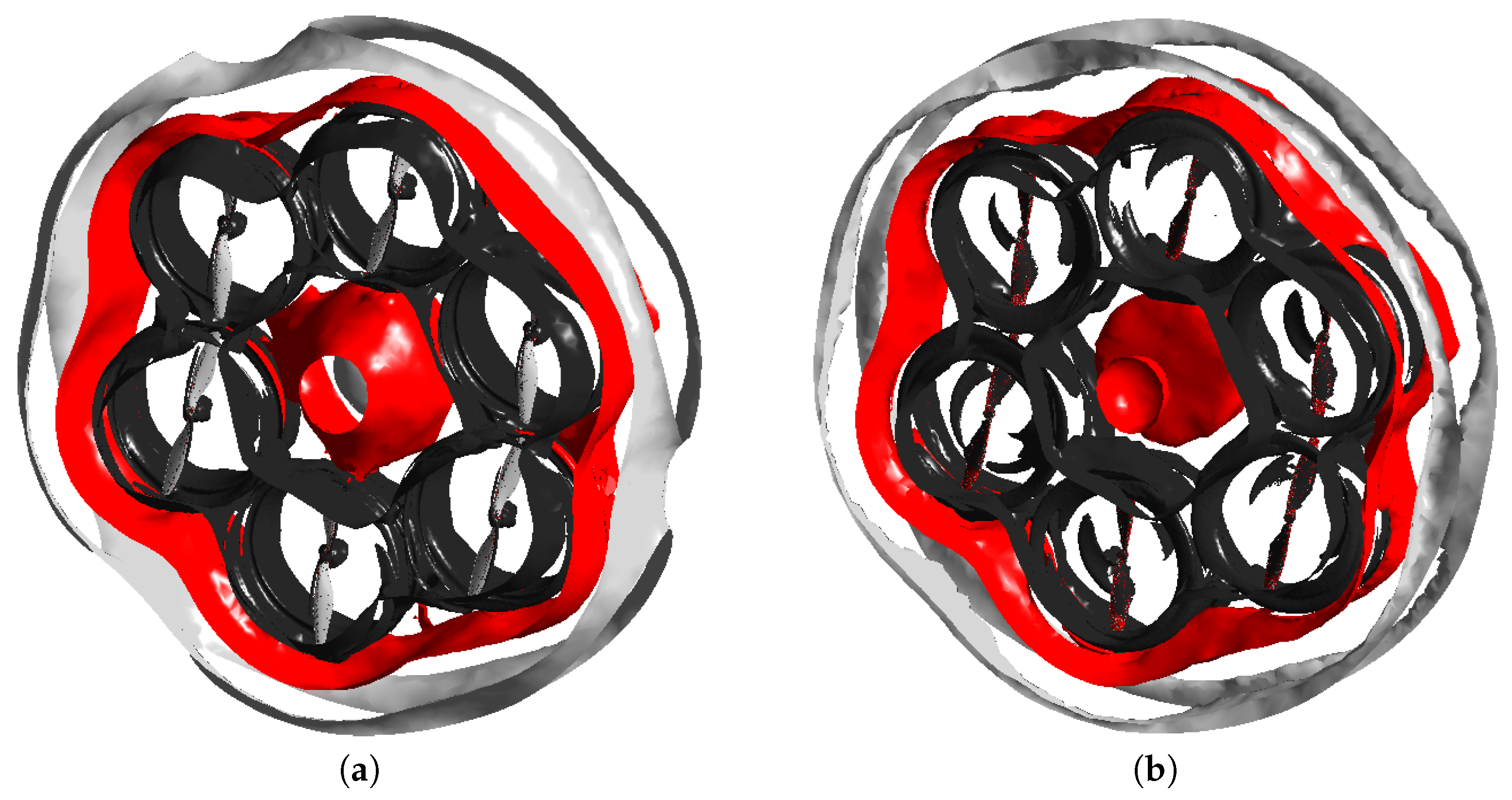
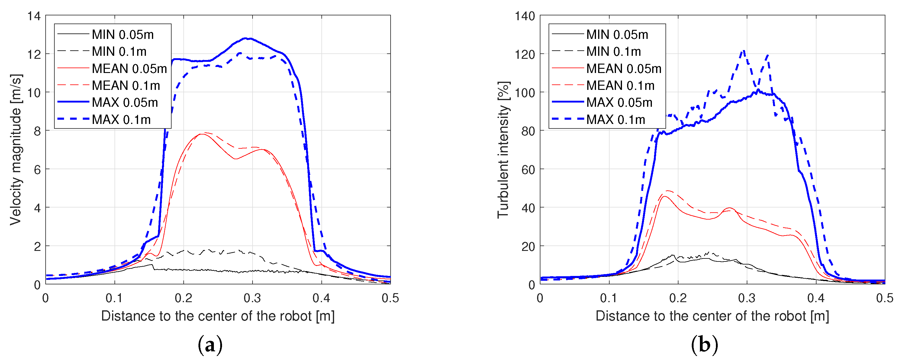
2.2. CFD Results and Design Decisions

The modeling process was carried out to obtain information about a phenomenon that is very difficult or even impossible to determine experimentally. The examples of such are, i.a., the distributions of velocity and turbulent intensity. These data in the form of isosurface visualization are presented in Figure 3.

The following procedure was applied to determine the best possible inlet location of the measurement system (first presented in [37] and used there for comparison of the rotor configurations). In the postprocessing stage, and using the polar coordinate system, the control points were placed in circles of increasing radii with a step of 0.001 m. A constant quantity of 500 points was kept in each circle. At all points, the values of the flow field parameters were read. For each of the circles, the maximum (MAX), minimum (MIN), and mean (MEAN) values of these were summarized in Figure 4. These points are placed in two planes located 0.05 m and 0.10 m, below and parallel to the rotor plane. These distances correspond to the location of the motor mounting and the extended arm surfaces, respectively. The greatest values occur at distances of about 0.15 m to 0.4 m from the robot’s center, that is, directly under the rotors.

The values of the radii for which the MIN, MAX, and MEAN field parameter values are similar in magnitude are areas where the influence of rotors on the flow field is insignificant. In particular, for the velocity magnitude, the difference between the MEAN and MAX values disappears almost completely for a value of about 1.0 $\mathrm{m}/\mathrm{s}$. Based on the analysis of the parameters indicated in Figure 4, it was decided to adopt the criterion of not exceeding the maximum velocity magnitude. For $V_{max}$, three thresholds $V_t$ were considered $V_{max}<V_t$, that is: 0.5, 1.0, and 2.0 $\mathrm{m}/\mathrm{s}$. Since the flow velocity is maximal within a limited range, two radius values r were found for these thresholds, that is, $r_{min}$ and $r_{max}$ for which the threshold value is exceeded. In other words, the flow velocity is greater than the threshold for a radius smaller than $r_{min}$ and greater than $r_{max}$. The results for both sections analyzed are summarized in

Table 1. Parameters in the sections analyzed for selected velocity magnitude thresholds.

${\mathit{V}}_{\mathit{t}}$	Section	${\mathit{r}}_{\mathit{min}}$	${\mathit{r}}_{\mathit{max}}$	${\mathit{I}}_{\mathit{max}}\left({\mathit{r}}_{\mathit{min}}\right)$	${\mathit{I}}_{\mathit{max}}\left({\mathit{r}}_{\mathit{max}}\right)$
0.5 $\mathrm{m}/\mathrm{s}$	0.05 m	0.065 m	0.470 m	3.98%	1.87%
	0.10 m	0.032 m	0.448 m	2.52%	2.58%
1.0 $\mathrm{m}/\mathrm{s}$	0.05 m	0.118 m	0.428 m	6.71%	3.77%
	0.10 m	0.105 m	0.421 m	5.33%	11.6%
2.0 $\mathrm{m}/\mathrm{s}$	0.05 m	0.144 m	0.389 m	24.2%	45.5%
	0.10 m	0.142 m	0.404 m	33.6%	41.1%

. The table also includes the values of $I_{max}$ of the maximum turbulent intensity for the given radii.

It was decided to adopt the $V_t$ threshold value equal to 1.0 $\mathrm{m}/\mathrm{s}$. This value was the most appropriate since for the 0.5 $\mathrm{m}/\mathrm{s}$ threshold the found radii are practically within the boundaries of the computational domain. On the other hand, for the 2.0 $\mathrm{m}/\mathrm{s}$ threshold, the turbulence intensities are in the range from 24.2% to 41.1%, so they are a very high case. When the turbulence intensity is also taken into account, the inlet of the measuring system should be located:

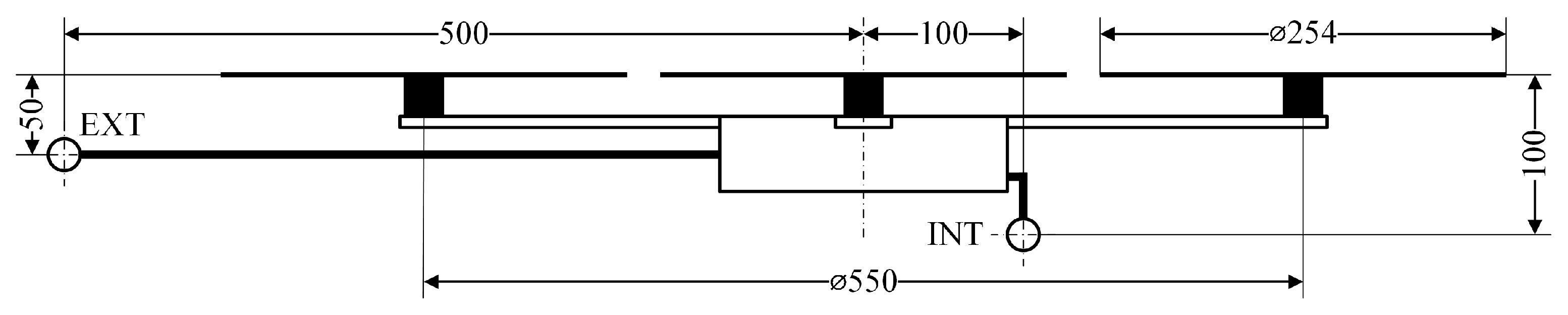
• Under the robot—0.10 m under the rotors’ plane, not further than 0.105 m. For this radius, the maximum turbulent intensity does not exceed 5.33%;
• On the extended arm—0.05 m below the rotors’ plane, at a distance greater than 0.428 m. For this radius, the maximum turbulent intensity does not exceed 3.77%.

During the construction of the prototype, it was decided to further investigate two locations for the inlet of the robot’s measurement system. According to the guidelines given, the inlet below the robot was located 0.10 m below the rotors’ plane and 0.10 m from the robot center of gravity (COG). The maximum value of the turbulent intensity for this location is 4.80%. The extended arm inlet was located 0.05 m below the rotors’ plane and 0.50 m from the COG where the maximum value of turbulent intensity was 1.96%.

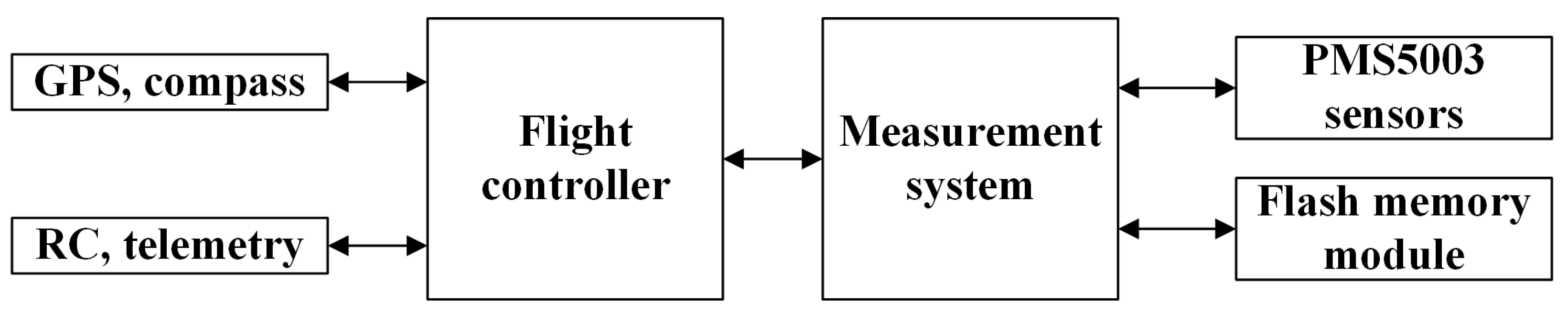
2.3. Final Prototype of the Measurement System

The final design robot has six drive sets, which include: EMAX MT2213 BLDC motors, 30 A ESCs, and 10 inch propellers. The maximum external dimensions of the robot are approximately 0.81 m × 0.81 m × 0.23 m. The robot is equipped with 2 identical high-current lithium polymer batteries (LiPo) with a nominal voltage of 11.1 V and a total capacity of 13 Ah. The weight of the robot with the measurement and control system is 2.54 kg, which does not exceed its lifting capacity of about 5 kg and allows for up to 25 min of flight.

The robot was equipped with two identical low-cost Plantower PMS5003 sensors. Their inlet locations are marked in Figure 5 as INT and EXT, which means internal and external. The sensors were mounted directly to the supporting structure without inlet extrusions to not adversely affect their measurement properties. The selected sensors are characterized by an active air intake system and a low overall response time. With these benefits, the robot can move faster and spend less time at the designated measurement points. The main sensor properties provided by the manufacturer are: measuring range 0.3 – 1.0, 1.0–2.5, and 2.5–10.0 $\mathsf{\mu }$m, counting efficiency of 50% for particle sizes 0.3 $\mathsf{\mu }$m and 98% for greater than 0.5 $\mathsf{\mu }$m, resolution 1 $\mathsf{\mu }$$\mathrm{g}/{\mathrm{m}}^3$, and total response time less than 10 s. The external dimensions of the sensor are 50 mm × 38 mm × 21 mm, and weight is about 38 g.

A simplified block diagram of the robot is presented in Figure 6. The robot was equipped with a flight controller and a prepared measurement and control system. The measurement and control system has external dimensions of about 0.12 m × 0.12 m × 0.04 m, it is powered by an independent converter, and its total mass with a PMS5003 sensor is about 0.33 kg. The key components of the system, apart from the microcontroller, are the fast flash memory that allows data recording, and the particle sensors. Additionally, the robot was fitted with a ready-made Pixhawk flight controller that is responsible for keeping the robot in the air. The measurement and control system takes measurements and directs the robot to the required coordinates. The robot was also equipped with additional components, such as GPS, RC receiver, telemetry radio, or battery monitor. Equipping the robot with a ready-made flight controller was a practical measure due to the simplification of the structure by dividing the functions directly related to the flight and the algorithm of searching for the source of pollution or PM measurements. Communication between the two controllers in the hardware layer takes place using the UART interface. For the software side, the Mavlink protocol was used.

3. Experimental Results

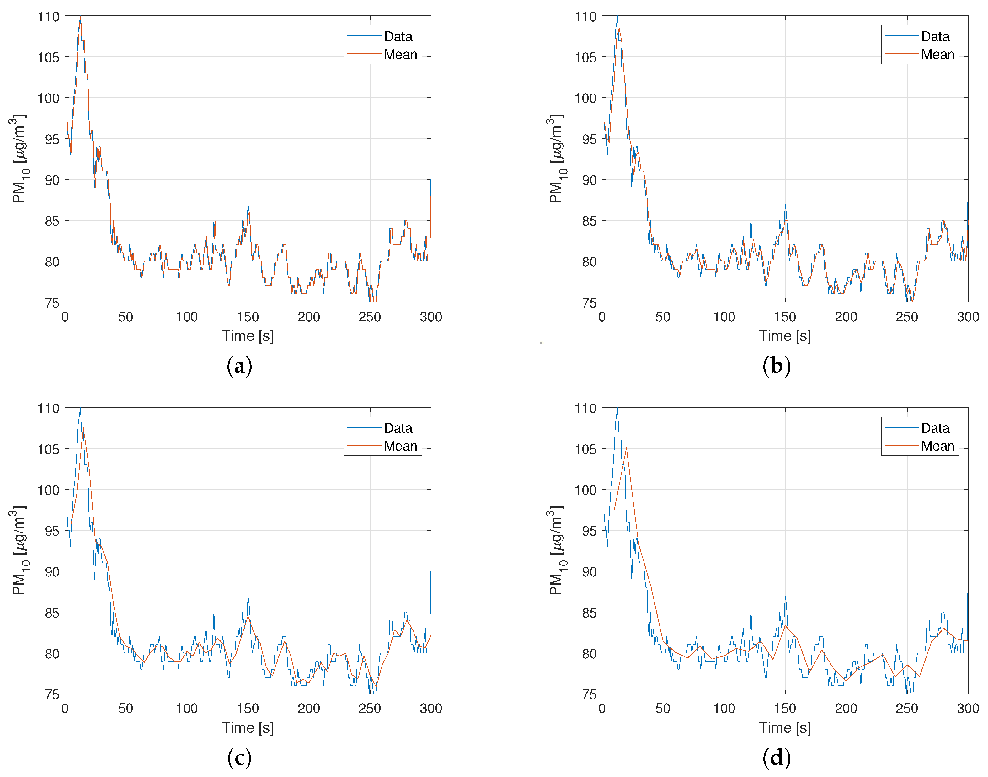
3.1. Measurement System Analysis

The analysis of the measurement data collected by the particulate matter sensors began with evaluating the properties of the sensors themselves. The sensors were found to have a variable sampling frequency that increased with higher levels of measured concentration. The measured ${\mathrm{PM}}_{10}$ concentration, which includes all particles counted by the sensor, was analyzed over time and is presented in Figure 7. The minimum, maximum, and average sampling frequencies were found to be 1.087 Hz, 1.191 Hz, and 1.123 Hz, respectively. This behavior of the sensors presents an additional challenge when comparing data from multiple independently operating sensors. To synchronize the data from various sensors, it was decided to determine the mean and median of the data for selected averaging periods.

The analysis was designed to examine the measurement properties of the sensors used and to select the appropriate averaging period. As there were no significant differences between the two versions, it was decided to use the mean, not the median. As the sensor is mounted on a multirotor robot, the averaging time cannot be too long. Based on the data presented, the most appropriate value is in the 2 s to 5 s range. The value of 3 s for the averaging time was adopted. When this value was taken into account, the concentrations were measured first in a closed room with the use of two identical sensors. The concentration data for ${\mathrm{PM}}_{1.0}$, ${\mathrm{PM}}_{2.5}$, and ${\mathrm{PM}}_{10}$ were recorded in 10 min. The results for ${\mathrm{PM}}_{10}$ are presented in Figure 8. On the basis of these data, an analysis was performed to verify that the obtained distributions have the character of a normal distribution. The graphic analysis is presented in Figure 8c,d in the form of a histogram and a quantile graph. In particular, based on Figure 8d, it should be assumed that the data are normal in a practical sense. Furthermore, the statistical parameters were determined and summarized in

Table 2. Statistical data determined for two PMS5003 sensors tested.

Parameter	INT			EXT
	${\mathrm{PM}}_{1.0}$	${\mathrm{PM}}_{2.5}$	${\mathrm{PM}}_{10}$	${\mathrm{PM}}_{1.0}$	${\mathrm{PM}}_{2.5}$	${\mathrm{PM}}_{10}$
Mean [$\mathsf{\mu }$$\mathrm{g}/{\mathrm{m}}^3$]	13.38	21.39	24.70	11.93	19.88	21.76
Standard deviation [$\mathsf{\mu }$$\mathrm{g}/{\mathrm{m}}^3$]	1.03	1.82	1.89	0.74	1.87	2.02
Expanded uncertainty [$\mathsf{\mu }$$\mathrm{g}/{\mathrm{m}}^3$]	0.15	0.26	0.27	0.10	0.26	0.29

.

The average sampling rates for this example were 1.1476 Hz and 1.1560 Hz, and the numbers of samples collected was 687 and 692, respectively. After averaging, the number of samples was equal to 200 for both sensors. With such a large number of observations, the coverage factor was assumed to be 2.0 to obtain a confidence interval of 95.45%. Based on Table 2, it should also be noted that the concentration of ${\mathrm{PM}}_{10}$ is the highest and that ${\mathrm{PM}}_{1.0}$ is the lowest. This is because the ${\mathrm{PM}}_{2.5}$ particles include the ${\mathrm{PM}}_{1.0}$ particles, and the ${\mathrm{PM}}_{10}$ particles include both ${\mathrm{PM}}_{2.5}$ and ${\mathrm{PM}}_{1.0}$ in the same way.

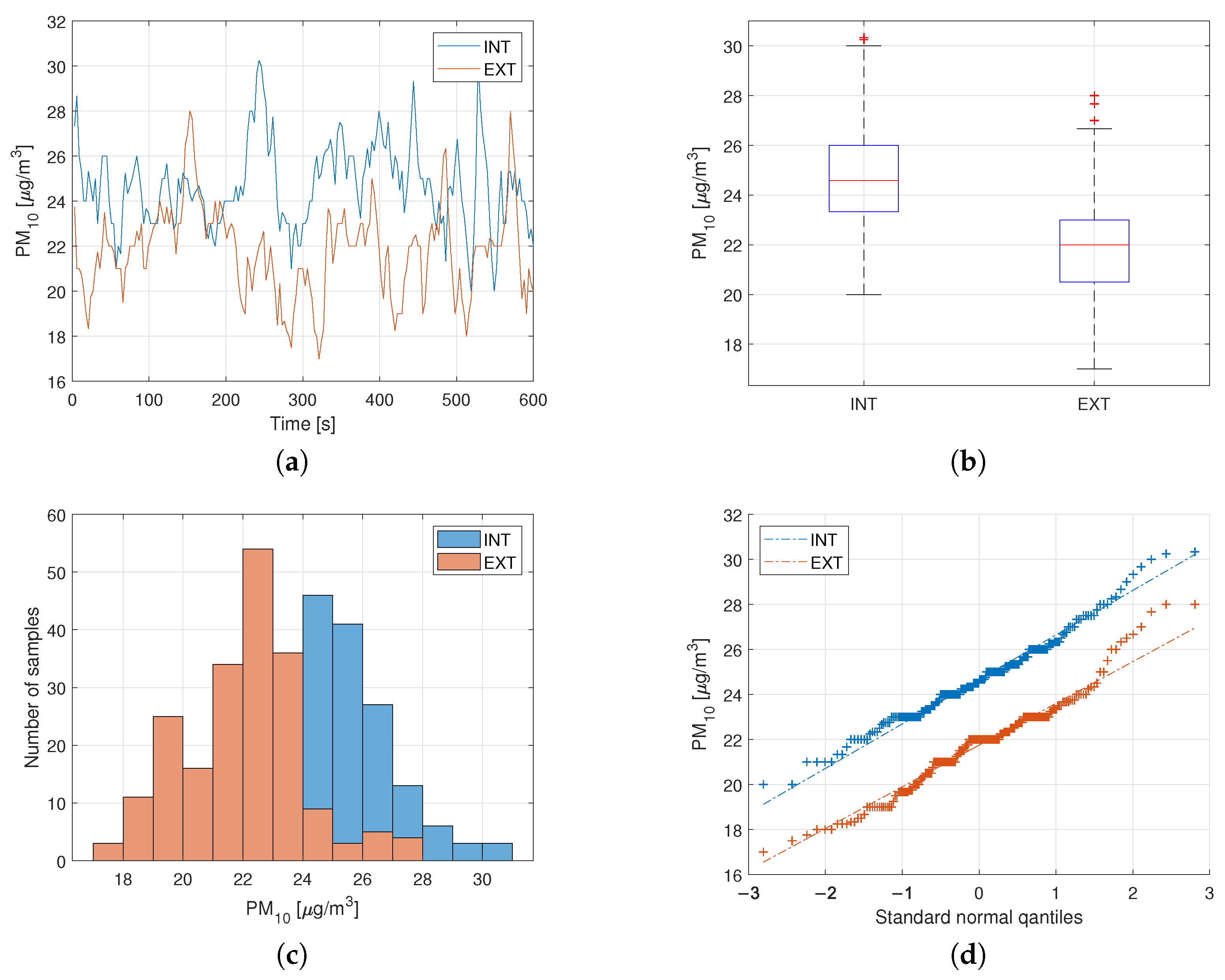
3.2. System Validation in Field Conditions

Field testing was carried out in flat areas without buildings, traffic, or bystanders. For measurements with a pollution source, the source was a small gastronomic grill located at a height of 0.5 m. During the tests, the robot maintained a constant altitude of about 4 m above ground level, and the horizontal speed of the robot was limited to 1.0 $\mathrm{m}/\mathrm{s}$. In addition, the robot also kept a constant orientation; that is, the nose (front) is to the north. Constant orientation was prepared in light of the fact that the sensor position at the end of the extended arm can be very easily determined by adding a constant value to the current position of the robot. In the case of measurements on a pole, the robot was located at a height similar to that when hovering. Measurements were made for the robot in a hovering state, stationary on a pole, and moving along various trajectories. In the cases where a pollution source was present, the robot also moved along the trajectories to find it.

Earlier analyses allowed us to indicate the proper way to process measurement data. With this knowledge in mind, a number of field measurements were performed for different atmospheric conditions and different average background concentrations of solid particles. The data were classified into three main groups, i.e., measurements made without the source of pollution during the flight and on the pole and measurements with the pollution source present. Figure 9, Figure 10 and Figure 11 present the collected data in the form of histograms and scatter plots with Pearson’s correlation coefficients determined. The results of ${\mathrm{PM}}_{10}$ from the first measurements, when the source of pollution was absent, were compared with those obtained from the nearby ground station, and the differences do not exceed 10%. Placing a reliable commercial grade particle counter on a drone is a difficult technical challenge and will be covered in future research.

The most important aspect of the research was to check the presence of strong linear correlations, independent of external conditions or the robot’s trajectory. The figures presented confirm the existence of such a relationship. The high internal correlation of the sensors results from including smaller-diameter particle measurements in larger-diameter particle measurements. The relationship discussed becomes even stronger under operating conditions of the rotors and when a pollution source is present. This is because both the speed of the air flow and the contaminants it contains, caused by the movement of the rotors, are dominant in relation to the speed of the air flowing around the drone.

When the source of the pollution was present, the histograms clearly showed more values at the ambient concentration level compared to the extreme values. These are background concentrations, while extreme values occurred during the robot’s contact with the pollution plume. The correlation of the internal values of the sensor concentrations, which also occurs in this case, is divided into two separate groups because of different types of contamination, namely the stage of the combustion process. It is most noticeable for the smallest particles (${\mathrm{PM}}_{1.0}$ and ${\mathrm{PM}}_{2.5}$).

Table 3. Summary of data collected under field conditions.

Rotors State	Pollution Source	Total Time	${\mathbf{PM}}_{10}$ Coefficients		${\mathbf{R}}^2$
			a	b
OFF	ABSENT	57 min 30 s	0.5970	14.3742	0.55
ON	ABSENT	72 min 54 s	0.7362	8.5585	0.87
	PRESENT	90 min 45 s	1.1984	4.9370	0.70

summarizes the total measurement time and the coefficients of the linear dependence equation

$${\mathrm{PM}}_{10,\mathrm{int}}=a·{\mathrm{PM}}_{10,\mathrm{ext}}+b$$

(7)

where ${\mathrm{PM}}_{10,\mathrm{int}}$ is an internal measurement, and ${\mathrm{PM}}_{10,\mathrm{ext}}$ is an external measurement.

Note that the highest value of the determination coefficient occurs for cases where the robot’s rotors are turned on. The determination coefficient (Table 3) indicates that with the rotors turned off, the results were less correlated (55%), compared to the rotors turned on (more than 70%). This means that the difference between sensor readings increases under such conditions. In the case of the concentration of ${\mathrm{PM}}_{10}$ covering all the measured particles, the concentrations on the internal sensor are overstated relative to the external sensor. Therefore, an internal sensor is more appropriate to find the source of the pollution. Both the occurrence and the proven correctness of such a relationship prove that on the basis of the measurement from one of the sensors, it is possible to estimate the value of the other one.

4. Conclusions

In summary, a prototype of a measurement system for an autonomous multirotor flying robot dedicated to searching for sources of air pollution was designed and tested under field conditions. The design of the measurement system incorporated energy-efficient considerations, such as the sensitivity of the system to contamination, to minimize the required flight time of the drone and ultimately reduce energy consumption. The effectiveness of the measurement system was achieved using a flow field computer model, which was built using the finite-volume method implemented in the numerical simulation software Ansys Fluent. Based on the data from the model, a novel criterion was proposed and applied that allowed the selection of the most appropriate locations of the measurement system inlet. It indicated the second placement within the space restricted by the rotors underneath the robot, in addition to the first most prominent placement on the extended arm. The measurement properties of the two PM sensors used were then investigated to determine their performance. This part of the work also proposes an appropriate method to process measurement data and defines guidelines for field research. Validation experiments were conducted first indoors at a constant concentration and then outdoors at a different level of background concentration and different atmospheric conditions. Field tests were carried out in three categories: movement with stationary rotors, flights with a pollution source present, and flights without a pollution source present, with the robot following various trajectories. The data collected revealed strong correlations between the readings from both sensors, regardless of external conditions or the robot’s trajectory. The field results confirm the validity of the conclusions drawn from the model analysis. Furthermore, when effectively searching for sources of pollution, the internal sensor located under the robot was found to be definitely better.

An important direction for further research, in addition to improving the accuracy of measurements, is the complex analysis of the possibility of recognizing the type of burnt elements based on the data of both sensors because the correlation of sensor indications in the case of the presence of a pollution source was clearly divided into two separate groups. Some aspects of modeling can also be improved, for example, by using a larger computational domain or the sliding mesh method. It is also important to confirm the assumed negligible influence of the robot body by including it in the model. Furthermore, the design procedure presented in this article with a slight modification can be applied to a drone measurement system that searches for many other sources of anthropological and natural air pollution. Another series of verification tests are planned in which the robot will first navigate using its internal sensor and then using its external one. Further research is planned to verify the applicability of the observed correlations and conclusions to other types of PM sensors, which may employ different measurement methods. The operation of both sensors for different pollution source search algorithms will also be verified. After this, the energy efficiency of the proposed solution can be quantitatively estimated. Optimization of the robot’s frame in order to minimize its weight should also be considered, as this will extend the flight time.

References

1. Murray, C.J.L.; Aravkin, A.Y.; Zheng, P.; Abbafati, C.; Abbas, K.M.; Abbasi-Kangevari, M.; Abd-Allah, F.; Abdelalim, A.; Abdollahi, M.; Abdollahpour, I.; et al. Global burden of 87 risk factors in 204 countries and territories, 1990–2019: A systematic analysis for the Global Burden of Disease Study 2019. Lancet 2020, 396, 1223–1249. [Google Scholar] [CrossRef]
2. Yang, T.; Zhou, K.; Ding, T. Air pollution impacts on public health: Evidence from 110 cities in Yangtze River Economic Belt of China. Sci. Total Environ. 2022, 851, 158125. [Google Scholar] [CrossRef] [PubMed]
3. Song, B.; Zhang, H.; Jiao, L.; Jing, Z.; Li, H.; Wu, S. Effect of high-level fine particulate matter and its interaction with meteorological factors on AECOPD in Shijiazhuang, China. Sci. Rep. 2022, 12, 8711. [Google Scholar] [CrossRef] [PubMed]
4. Chandia-Poblete, D.; Cole-Hunter, T.; Haswell, M.; Heesch, K.C. The influence of air pollution exposure on the short- and long-term health benefits associated with active mobility: A systematic review. Sci. Total Environ. 2022, 850, 157978. [Google Scholar] [CrossRef] [PubMed]
5. Duangsuwan, S.; Jamjareekulgarn, P. Development of drone real-time air pollution monitoring for mobile smart sensing in areas with poor accessibility. Sens. Mater. 2020, 32, 511–520. [Google Scholar] [CrossRef] [Green Version]
6. Fan, M.; Zhang, L. The Design of Multirotor Aircraft-based Environmental Detection System. MATEC Web Conf. 2018, 232, 04082. [Google Scholar] [CrossRef]
7. Shah, S.N.; Xiong, X. Balluino: High Altitude Balloon/Drone Based Air Pollution and PM 2.5 Monitoring System. In Proceedings of the 2019 IEEE Long Island Systems, Applications and Technology Conference (LISAT), Long Island, NY, USA, 3 May 2019; pp. 1–5. [Google Scholar] [CrossRef]
8. Li, X.B.; Peng, Z.R.; Lu, Q.C.; Wang, D.; Hu, X.M.; Wang, D.; Li, B.; Fu, Q.; Xiu, G.; He, H. Evaluation of unmanned aerial system in measuring lower tropospheric ozone and fine aerosol particles using portable monitors. Atmos. Environ. 2020, 222, 117134. [Google Scholar] [CrossRef]
9. Li, X.B.; Wang, D.S.; Lu, Q.C.; Peng, Z.R.; Wang, Z.Y. Investigating vertical distribution patterns of lower tropospheric PM2.5 using unmanned aerial vehicle measurements. Atmos. Environ. 2018, 173, 62–71. [Google Scholar] [CrossRef]
10. Aurell, J.; Gullett, B.; Holder, A.; Kiros, F.; Mitchell, W.; Watts, A.; Ottmar, R. Wildland fire emission sampling at Fishlake National Forest, Utah using an unmanned aircraft system. Atmos. Environ. 2021, 247, 118193. [Google Scholar] [CrossRef]
11. Kobziar, L.N.; Pingree, M.R.A.; Watts, A.C.; Nelson, K.N.; Dreaden, T.J.; Ridout, M. Accessing the Life in Smoke: A New Application of Unmanned Aircraft Systems (UAS) to Sample Wildland Fire Bioaerosol Emissions and Their Environment. Fire 2019, 2, 56. [Google Scholar] [CrossRef] [Green Version]
12. Bieber, P.; Seifried, T.M.; Burkart, J.; Gratzl, J.; Kasper-Giebl, A.; Schmale, D.G.; Grothe, H. A Drone-Based Bioaerosol Sampling System to Monitor Ice Nucleation Particles in the Lower Atmosphere. Remote Sens. 2020, 12, 552. [Google Scholar] [CrossRef] [Green Version]
13. Sasaki, K.; Inoue, M.; Shimura, T.; Iguchi, M. In Situ, Rotor-Based Drone Measurement of Wind Vector and Aerosol Concentration in Volcanic Areas. Atmosphere 2021, 12, 376. [Google Scholar] [CrossRef]
14. Mahanteshaiah, M.K.; Holla, S.A.; Nirahankar, K.S.; Sivan, A.; Purushotham, G. Environmental pollution control using artificial intelligence drone. AIP Conf. Proc. 2020, 2311, 030031. [Google Scholar] [CrossRef]
15. Bretschneider, L.; Schlerf, A.; Baum, A.; Bohlius, H.; Buchholz, M.; Düsing, S.; Ebert, V.; Erraji, H.; Frost, P.; Käthner, R.; et al. MesSBAR—Multicopter and Instrumentation for Air Quality Research. Atmosphere 2022, 13, 629. [Google Scholar] [CrossRef]
16. Wu, C.; Liu, B.; Wu, D.; Yang, H.; Mao, X.; Tan, J.; Liang, Y.; Sun, J.Y.; Xia, R.; Sun, J.; et al. Vertical profiling of black carbon and ozone using a multicopter unmanned aerial vehicle (UAV) in urban Shenzhen of South China. Sci. Total Environ. 2021, 801, 149689. [Google Scholar] [CrossRef] [PubMed]
17. Chang, C.C.; Chang, C.Y.; Wang, J.L.; Pan, X.X.; Chen, Y.C.; Ho, Y.J. An optimized multicopter UAV sounding technique (MUST) for probing comprehensive atmospheric variables. Chemosphere 2020, 254, 126867. [Google Scholar] [CrossRef]
18. Aurell, J.; Mitchell, W.; Chirayath, V.; Jonsson, J.; Tabor, D.; Gullett, B. Field determination of multipollutant, open area combustion source emission factors with a hexacopter unmanned aerial vehicle. Atmos. Environ. 2017, 166, 433–440. [Google Scholar] [CrossRef]
19. Lee, S.H.; Kwak, K.H. Assessing 3-D Spatial Extent of Near-Road Air Pollution around a Signalized Intersection Using Drone Monitoring and WRF-CFD Modeling. Int. J. Environ. Res. Public Health 2020, 17, 6915. [Google Scholar] [CrossRef]
20. Kuuluvainen, H.; Poikkimäki, M.; Järvinen, A.; Kuula, J.; Irjala, M.; Dal Maso, M.; Keskinen, J.; Timonen, H.; Niemi, J.V.; Rönkkö, T. Vertical profiles of lung deposited surface area concentration of particulate matter measured with a drone in a street canyon. Environ. Pollut. 2018, 241, 96–105. [Google Scholar] [CrossRef]
21. Cozma, A.; Firculescu, A.C.; Tudose, D.; Ruse, L. Autonomous Multi-Rotor Aerial Platform for Air Pollution Monitoring. Sensors 2022, 22, 860. [Google Scholar] [CrossRef]
22. Pochwała, S.; Gardecki, A.; Lewandowski, P.; Somogyi, V.; Anweiler, S. Developing of Low-Cost Air Pollution Sensor—Measurements with the Unmanned Aerial Vehicles in Poland. Sensors 2020, 20, 3582. [Google Scholar] [CrossRef] [PubMed]
23. Madokoro, H.; Kiguchi, O.; Nagayoshi, T.; Chiba, T.; Inoue, M.; Chiyonobu, S.; Nix, S.; Woo, H.; Sato, K. Development of Drone-Mounted Multiple Sensing System with Advanced Mobility for In Situ Atmospheric Measurement: A Case Study Focusing on PM2.5 Local Distribution. Sensors 2021, 21, 4881. [Google Scholar] [CrossRef] [PubMed]
24. Hedworth, H.A.; Sayahi, T.; Kelly, K.E.; Saad, T. The effectiveness of drones in measuring particulate matter. J. Aerosol Sci. 2021, 152, 105702. [Google Scholar] [CrossRef]
25. Pochwała, S.; Anweiler, S.; Deptuła, A.; Gardecki, A.; Lewandowski, P.; Przysiężniuk, D. Optimization of air pollution measurements with unmanned aerial vehicle low-cost sensor based on an inductive knowledge management method. Optim. Eng. 2021, 22, 1783–1805. [Google Scholar] [CrossRef]
26. Alfano, B.; Barretta, L.; Del Giudice, A.; De Vito, S.; Di Francia, G.; Esposito, E.; Formisano, F.; Massera, E.; Miglietta, M.L.; Polichetti, T. A Review of Low-Cost Particulate Matter Sensors from the Developers’ Perspectives. Sensors 2020, 20, 6819. [Google Scholar] [CrossRef]
27. Jońca, J.; Pawnuk, M.; Bezyk, Y.; Arsen, A.; Sówka, I. Drone-Assisted Monitoring of Atmospheric Pollution: A Comprehensive Review. Sustainability 2022, 14, 11516. [Google Scholar] [CrossRef]
28. Amaral, S.S.; De Carvalho, J.A.; Costa, M.A.M.; Pinheiro, C. An Overview of Particulate Matter Measurement Instruments. Atmosphere 2015, 6, 1327–1345. [Google Scholar] [CrossRef] [Green Version]
29. Lee, H.; Kang, J.; Kim, S.; Im, Y.; Yoo, S.; Lee, D. Long-Term Evaluation and Calibration of Low-Cost Particulate Matter (PM) Sensor. Sensors 2020, 20, 3617. [Google Scholar] [CrossRef]
30. Stavroulas, I.; Grivas, G.; Michalopoulos, P.; Liakakou, E.; Bougiatioti, A.; Kalkavouras, P.; Fameli, K.M.; Hatzianastassiou, N.; Mihalopoulos, N.; Gerasopoulos, E. Field Evaluation of Low-Cost PM Sensors (Purple Air PA-II) Under Variable Urban Air Quality Conditions, in Greece. Atmosphere 2020, 11, 926. [Google Scholar] [CrossRef]
31. Kaliszewski, M.; Włodarski, M.; Młyńczak, J.; Kopczyński, K. Comparison of Low-Cost Particulate Matter Sensors for Indoor Air Monitoring during COVID-19 Lockdown. Sensors 2020, 20, 7290. [Google Scholar] [CrossRef]
32. Bulot, F.M.J.; Russell, H.S.; Rezaei, M.; Johnson, M.S.; Ossont, S.J.J.; Morris, A.K.R.; Basford, P.J.; Easton, N.H.C.; Foster, G.L.; Loxham, M.; et al. Laboratory Comparison of Low-Cost Particulate Matter Sensors to Measure Transient Events of Pollution. Sensors 2020, 20, 2219. [Google Scholar] [CrossRef] [PubMed] [Green Version]
33. Suchanek, G.; Wołoszyn, J.; Gołaś, A. Evaluation of Selected Algorithms for Air Pollution Source Localisation Using Drones. Sustainability 2022, 14, 3049. [Google Scholar] [CrossRef]
34. Jing, T.; Meng, Q.H.; Ishida, H. Recent Progress and Trend of Robot Odor Source Localization. IEEJ Trans. Electr. Electron. Eng. 2021, 16, 938–953. [Google Scholar] [CrossRef]
35. Suchanek, G.; Filipek, R. CFD analysis of a multi-rotor flying robot for air pollution inspection. J. Phys. Conf. Ser. 2022, 2367, 012010. [Google Scholar] [CrossRef]
36. Gosiewski, Z.; Kwaśniewski, K. Time Minimization of Rescue Action Realized by an Autonomous Vehicle. Electronics 2020, 9, 2099. [Google Scholar] [CrossRef]
37. Suchanek, G.; Filipek, R. Computational Fluid Dynamics (CFD) Aided Design of a Multi-rotor Flying Robot for Locating Sources of Particulate Matter Pollution. Appl. Comput. Sci. 2022, 18, 86–104. [Google Scholar] [CrossRef]
38. Batchelor, G.K. An Introduction to Fluid Dynamics; Cambridge University Press: Cambridge, UK, 1967. [Google Scholar]
39. Wilcox, D.C. Turbulence Modeling for CFD, 3rd ed.; DCW Industries: La Cañada, CA, USA, 2006. [Google Scholar]
40. Menter, F.R. Two-equation eddy-viscosity turbulence models for engineering applications. AIAA J. 1994, 32, 1598–1605. [Google Scholar] [CrossRef] [Green Version]
41. Romik, D.; Czajka, I. Numerical Investigation of the Sensitivity of the Acoustic Power Level to Changes in Selected Design Parameters of an Axial Fan. Energies 2022, 15, 1357. [Google Scholar] [CrossRef]
Figure 1. The six-rotor configuration: (a) geometric model; (b) boundary conditions—top view; (c) side view. Boundary conditions are as follows: pressure-inlet—1; pressure-outlet—2; interface—3; rotating-wall—4; dynamic zones—5; static zone—6.
Energies 16 02959 g001
Figure 2. The prepared mesh: (a) entire domain; (b) close-up on the boundary layer of the rotor.
Energies 16 02959 g002
Figure 3. Isosurface visualisation of the field parameter distribution: (a) velocity magnitude—0.3, 1.0, 3.0 m / s (grey, red, black); (b) turbulence intensity—1, 5, 14% (grey, red, black).
Energies 16 02959 g003
Figure 4. Minimum (MIN), maximum (MAX), and average (MEAN) values of parameters from the CFD computer model for sections located (0.05 m) and (0.1 m) under the rotors’ plane: (a) velocity magnitude; (b) turbulent intensity.
Energies 16 02959 g004
Figure 5. Final robot and measurement system schematic.
Energies 16 02959 g005
Figure 6. Simplified block diagram of the designed robot.
Energies 16 02959 g006
Figure 7. Raw data and average of PM 10 data from the single sensor for selected averaging periods: (a) 1 s; (b) 2 s; (c) 5 s; (d) 10 s.
Energies 16 02959 g007
Figure 8. PM 10 data from both sensors: (a) time series; (b) box plot; (c) histogram; (d) qq plot.
Energies 16 02959 g008
Figure 9. Histogram and correlation of measured PM concentrations without pollution source.
Energies 16 02959 g009
Figure 10. Histogram and correlation of measured PM concentrations without pollution source during flight.
Energies 16 02959 g010
Figure 11. Histogram and correlation of measured PM concentrations with the source of pollution during flight.
Energies 16 02959 g011